1. Introduction
Fixed wing aircraft performance is governed by aerodynamic efficiency. One way of increasing aerodynamic efficiency and thus range and endurance is to fly in the wake of another aircraft. Birds have used this effect before the first analyses on this flight method were conducted [
1]. The concept of flying in the trailing vortex has been a source of research for quite sometime [
2] with problems such as time-delay effects [
3] or self spacing issues [
4]. Although numerous work has been done on formation flight with benefits categorized, it is a potentially dangerous maneuver and quite costly in terms of control to ensure station keeping in such a turbulent flow regime [
5,
6,
7].
As such the topic of joined aircraft has been studied as opposed to formation flight [
8]. The performance benefits are still similar to formation flight in that range and endurance are increased. Joining aircraft at the wing tips reduces the effect of wing tip vortices and increases lift on each aircraft thus increasing aerodynamic performance. The flagship project for connected aircraft occurred post World War II codenamed Project TipTow [
9]. This experiment involved three aircraft. The center aircraft was a B-29 while two F-84s docked with both wingtips on the B-29. One of these flight tests exhibited an unstable oscillation which resulted in a failure and a pilot death. Not much work outside some windtunnel experiments and trade studies have been conducted since that project [
8,
10] however the Distributed Flight Array (DFA) offers the first successful flight using vertical take and landing aircraft [
11,
12]. The DFA is a set of ground rovers that contain one main rotor with no cyclic control. Thus, each individual ground robot cannot fly independently. Once the individual robots link together, the thrust from each rover can be controlled independently to ensure that the attitude and altitude of the conjoined flight array is stabilized.
The task of connecting multiple singular independent bodies has been investigated for quite some time. Resource management of multiple UAVs has been investigated for hostile territories showing the increase in efficiency by using multiple aircraft [
13,
14]. Modular or morphing robots have created interesting research problems including the development of reconfiguration algorithms [
15,
16] to completely reconfigure these types of robots. The control schemes for these robots includes adaptive control techniques [
17] as well as using some fault tolerant control techniques [
18,
19,
20] to handle reconfiguration of vehicles.
The challenge of connecting multiple fixed wing UAVs has been investigated quite recently by characterizing modes and modes shapes of connected aircraft [
21] which showed that certain configurations of meta aircraft are unstable while also highlighting the flexible modes of meta aircraft. Work as also been done on performance increase of meta aircraft as a function of configuration [
22]. Controllability has also been investigated [
23] with the result that all meta aircraft configurations are at least controllable. That is, if the controllability matrix is computed for any aircraft configuration, the matrix is full rank [
24]. The challenge of connecting in flight poses a difficult problem with the presence of atmospheric disturbances but using vision based feedback can help mitigate this problem [
25,
26]. Work has been done on unlinking UAVs mid-flight [
27] in support of the High Altitude Long Endurance (HALE) projects [
28] as well as Project Link [
26]! The simulation results from Project Link! showed that reconfigurable control laws are necessary for unlinking UAVs.
Although experiments have been done on multicopters [
11] or even highly flexible aircraft [
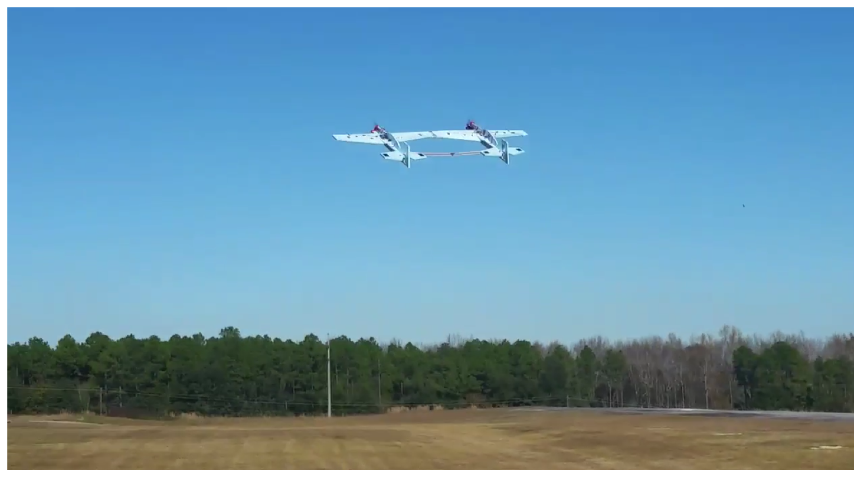
29], no work has been done on developing an experimental test bed to evaluate fixed wing simulation results. The report here describes an experimental test involving two autonomous fixed wing aircraft connected at the wing tips with magnets. The sections that follow describe the aircraft, the control system, some simulation results and finally flight test results.
2. Aircraft Design
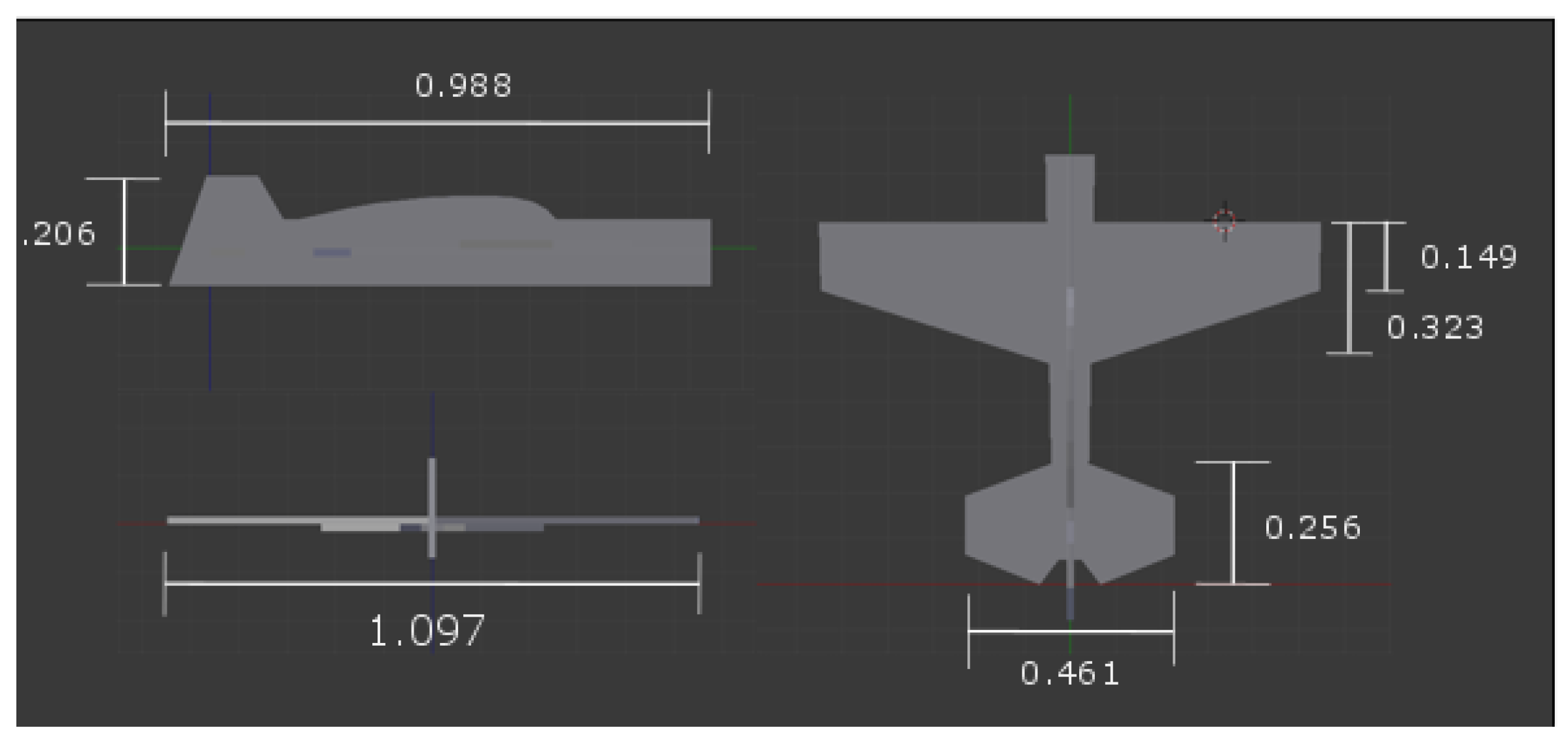
The general aerodynamic design of the aircraft was inspired by the Yak-54, which was designed for aerobatic competitions. The Yak-54 is a 3D flyer, which means it can fly straight up, upside down, and any other three-dimensional state. As such, the aircraft built is also a 3D flyer. This design was chosen because it is very stable and maneuverable. The design was downscaled to have a wingspan of 1.097 m. A schematic of the aircraft is shown in
Figure 1.
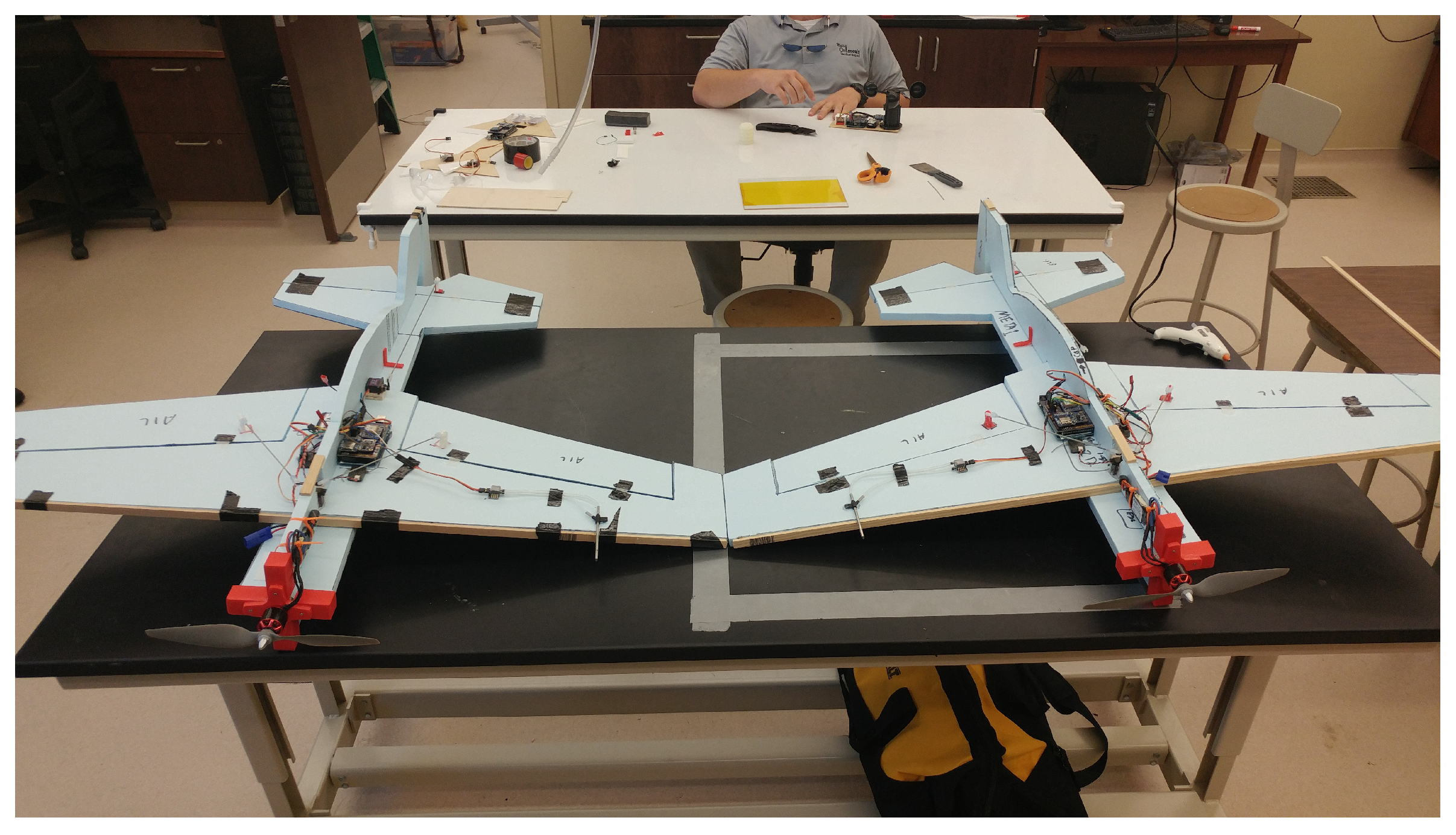
Two aircraft were constructed for the experimental flight. Building the aircraft in-house facilitated easy mounting of the autopilot system and wing tip connections. Standard off the shelf aircraft typically have little room to add extra electronics.
Figure 2 shows the two aircraft side by side. The aircraft were built out of 1 inch insulation foam which has a density of 0.0229 g/cm
. The total mass of the aircraft including the autopilot and connection mechanism were 818 g. The inertia of the aircraft are 0.073, 0.12, 0.182 kg·m
along the
x,
y and
z body axes respectively. The aircraft has only two standard control surfaces: ailerons and elevators. Simulation results revealed that rudder control is not needed for these aircraft. Each aircraft has independent throttle controlled by a single propeller mounted on the front of the aircraft.
The geometric properties of the aircraft were obtained by measuring the aircraft itself. The wingspan, chord and tail area can all be seen in
Figure 1. The aerodynamic properties were obtained by using flat plate theory for the wings [
30]. Since the aircraft itself was built out of 1 inch insulation foam this is a good approximation. The stability derivatives were obtained using standard aircraft stability theory [
31,
32]. The aerodynamic properties for this aircraft are shown in
Table 1.
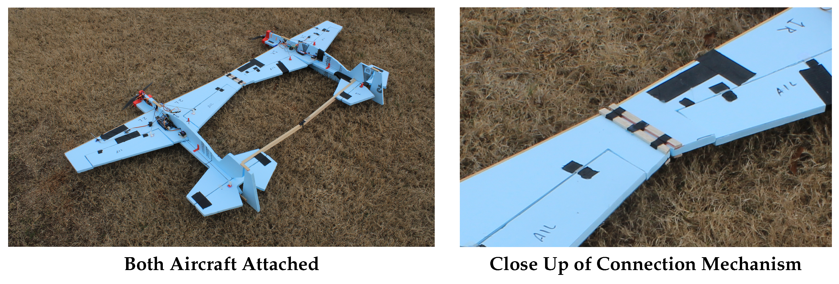
The connection mechanism of the aircraft was designed to be removable. Though all of the experimental testing in this article is done with already connected aircraft, the connection between the two aircraft was designed such that they could connect during a flight test and be separated later. The ability to separate also helped in transportation of the two aircraft. Three strong neodymium magnets were attached to the ends of the wingtips as shown in
Figure 3 (Right). The magnets allowed the aircraft to separate while also maintaining connection during flight. Each magnet was placed on the wingtips of both aircraft and has a connection force of 56.8 N. The magnets were chosen to be several times stronger than the weight of both aircraft (818 g∼8 N) to prevent the likelihood of a strong gust of wind separating them. Another requirement was that the magnets fit on the ends of the wing tips; therefore, the width was chosen to be 1.5 cm and the thickness to be a few millimeters so they do not protrude too far out of the wing. Weight was also an issue. Each magnet has a mass of 14.3 g which is small but the final design included 4 magnets for an increase of 57.2 g on the empty weight of the aircraft. Three magnets were placed on each wing tip and another magnet was placed on horizontal tail booms to reduce pitch oscillations between aircraft as shown in
Figure 3 (Left). The horizontal tail boom was added to reduce torsional stress on the main wings. However, because these were added the focus of simulation results and experimental results will be on roll excursions between aircraft.
3. Control System
The control system used seeks to keep the aircraft level in both pitch (
) and roll (
). The aileron (
) seeks to roll the aircraft to the desired roll angle command (
) which for the experiment presented here is set to zero. The pitch angle feedback is fed directly to the elevator (
) to ensure the pitch angle reaches the desired pitch angle command (
) which is set to a constant. Note that each aircraft has its own flight controller and each flight controller does not communicate with the other. The main goal for each aircraft is to reach the same pitch and roll angle to reach steady state flight in a multi-body configuration. The equations for the aileron and elevator for the
ith aircraft are shown below. The constants
and
are proportional and derivative gains.
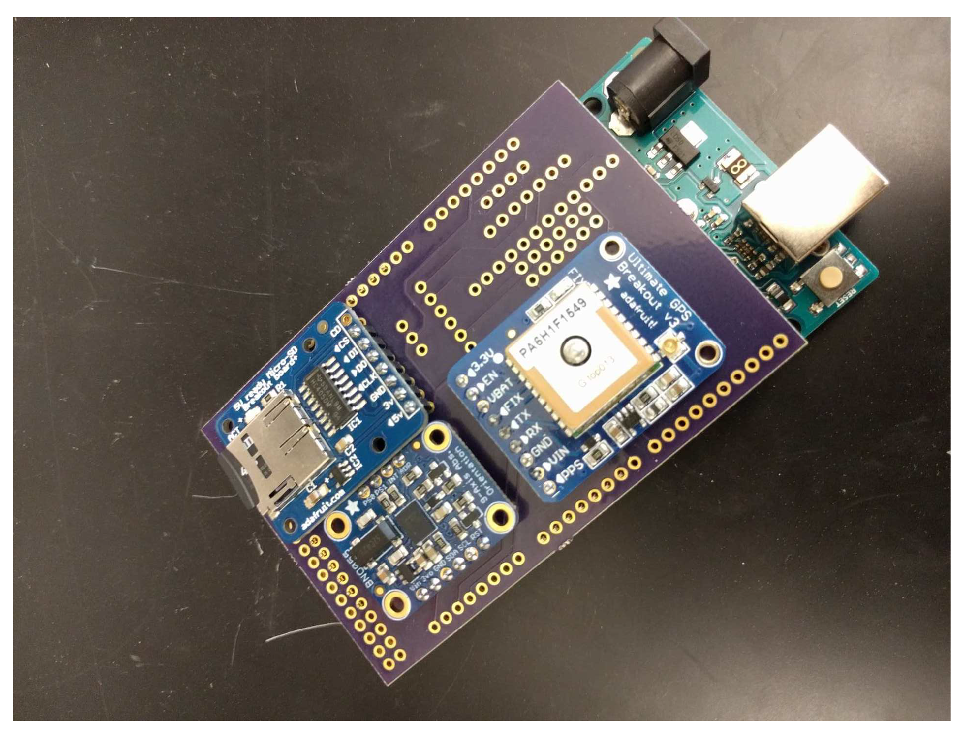
The onboard autopilot consists of an Arduino MEGA 2560 with a GPS, IMU (Inertial Measurement Unit), and SD card to log data. The Arduino MEGA 2560 utilizes an ATMega microchip that operates at 16 MHz. Each GPS module logged position and heading data as well as forward speed. The IMU is a 3 axis accelerometer, rate gyro and magnetometer capable of monitoring roll, pitch and yaw as well as angular rates. The magnetometer heading accuracy is rated to 2.5 degrees and the rate gyro has an output noise of 0.1 degree/s. The accelerometer is rated to
of zero-g offset. This IMU uses proprietary sensor fusion to give Euler angles at a rate of up to 100 Hz. This includes the derivatives of the Euler angles
and
. A picture of the autopilot system is shown in
Figure 4. The shield on top of the Arduino MEGA is the SD card reader, IMU and GPS starting from the top and moving in a counter clockwise direction.
In addition to having all the sensors necessary for control, the autopilot system features a small transistor array circuit (not pictured) using a series of NPN and PNP transistors. These transistors allow current to flow from one source and impede flow in another depending on the voltage of the base pin. This allows the pilot to manually control both airplanes with one transmitter and then flip a switch on the transmitter to allow the Arduino to control the aircraft. Thus, the transistors have two inputs: the signal from the pilot and the signal from the Arduino. This is done for the elevator and ailerons. The pilot constantly maintains control of the throttle and relinquishes control of the elevator and ailerons by activating the transistors. The gains in the PID controller are set to (. The same gains are used in both simulation and experiment. The gains were obtained experimentally by performing a few ground tests and some in flight tests.
4. Simulation Results
Example simulation results are presented for this system using the equations of motion defined in [
23]. The equations of motion use the standard six degree of freedom aircraft model [
33] combined with an elastic joint to model connection at the wingtips. The purpose of this simulation is to highlight some key issues with connected aircraft with the main issue being the ability for the two aircraft to attain distinct attitudes. That is, the vehicle does not behave like a rigid body since the connection joint is highly flexible. For the example simulation, the stiffness and damping values of the connection joint are set relatively low so that the simulation can be run in real time. Thus, the linear springs are set to
N/m. The damping coefficients are all set to the same value of
= 0.75 N·s/m. The rotational stiffness is set to 2.0 N·m/rad while the damping coefficient is set to 1.0 N·m/rad. The density of air is set to standard sea-level at 1.225 kg/m
. The simulation was tested with one aircraft at zero degrees and one with the aircraft at 50 degrees. The simulation proceeds with both aircraft traveling at 14 m/s initially with no control.
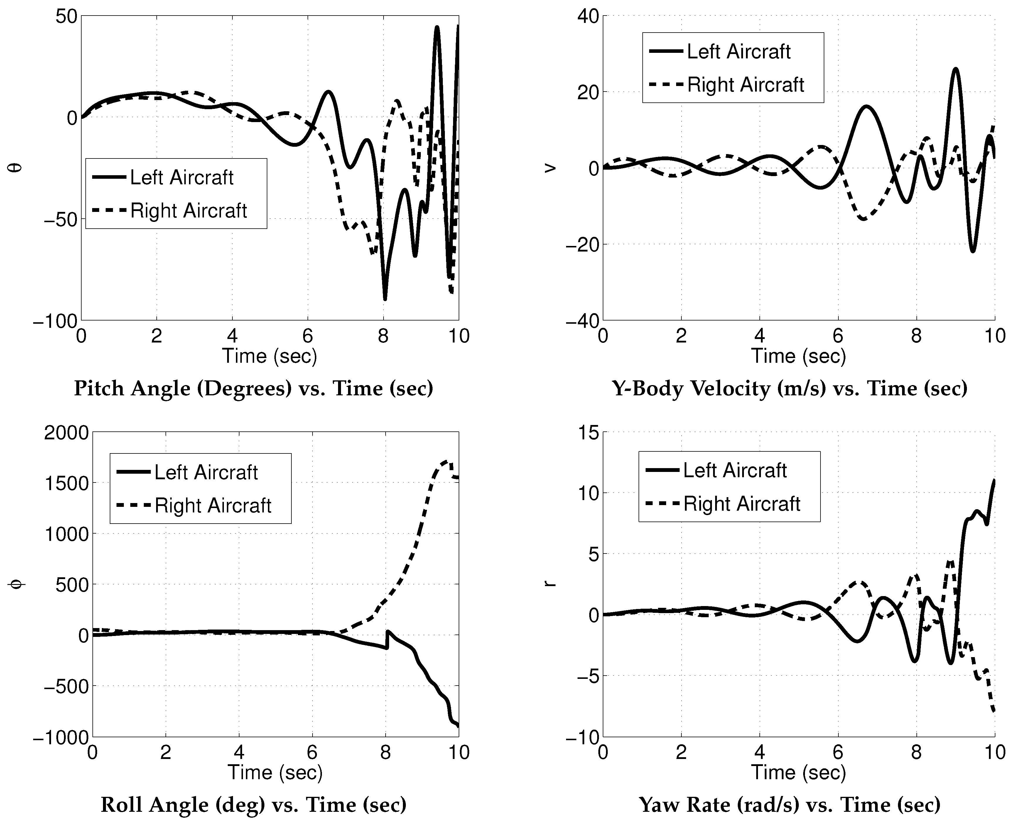
Figure 5 shows the pitch and roll angles as well as the yaw rate and side velocity of the aircraft without any control input from the pilot or the autopilot. The reason for these excursions is caused by a coupling between the roll and yaw dynamics of the aircraft. Compared to the roll angle, the pitch angle of the aircraft stay relatively close together. However, the yaw rate and sideslip oscillate out of phase much like a dutch roll mode and is unstable due to the coupling between the aerodynamics and the joint dynamics. When the left aircraft yaws negative, it generates a positive y body velocity. This can be seen as an increase in sideslip. In this case, the joint torque combined with the stabilizing aerodynamic torque from the vertical stabilizer restores the aircraft to straight and level. This however creates a positive yaw rate. Due to the asymmetry in the aircraft, the left aircraft would experience an increase in freestream velocity which would increase lift on the aircraft. This would thus increase the roll angle of the aircraft while it swings forward. This process repeats itself and leads to joint failure. This instability from the yaw and roll coupling gives rise to the large roll excursions that can be seen after 6 s.
The magnetic forces and moments from the torsional springs initially restore aircraft attitude equality but fail to maintain this after about 5 s. The roll angle deviation is so large here that the aircraft would separate in a real experiment. This unstable mode however, can be stabilized by using state feedback. The same initial values were given to the simulation with the autopilot on. The controller seeks to bring both aircraft’s roll angles to zero which would serve to fix the initial deviation in roll angle.
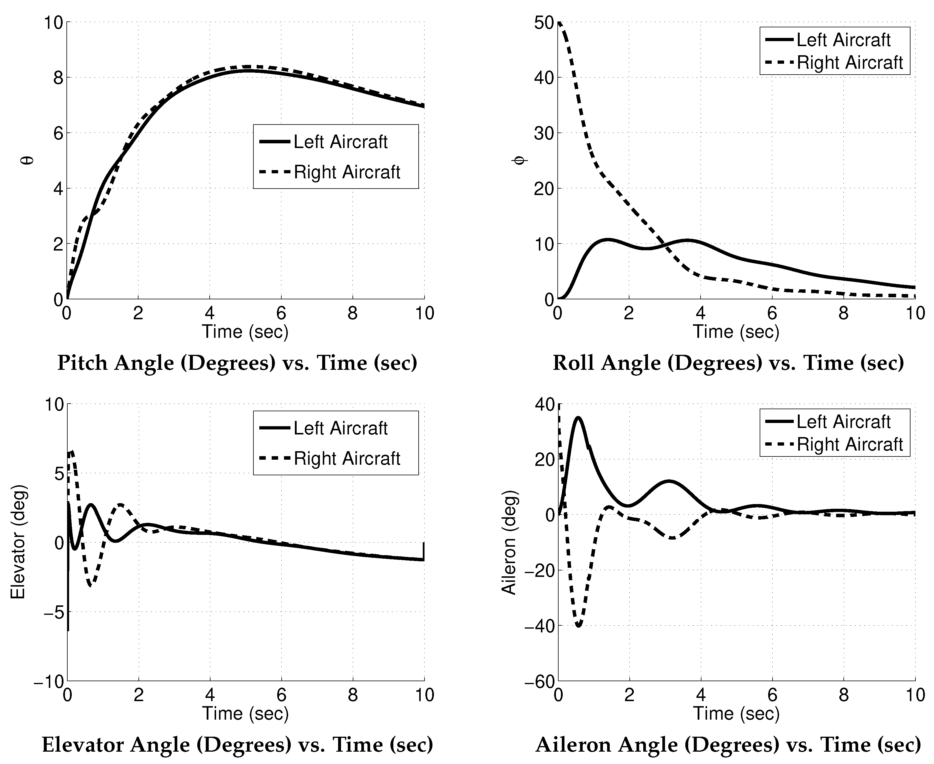
Figure 6 shows the closed loop results of the connected aircraft simulation.
The PID control law using Equation (
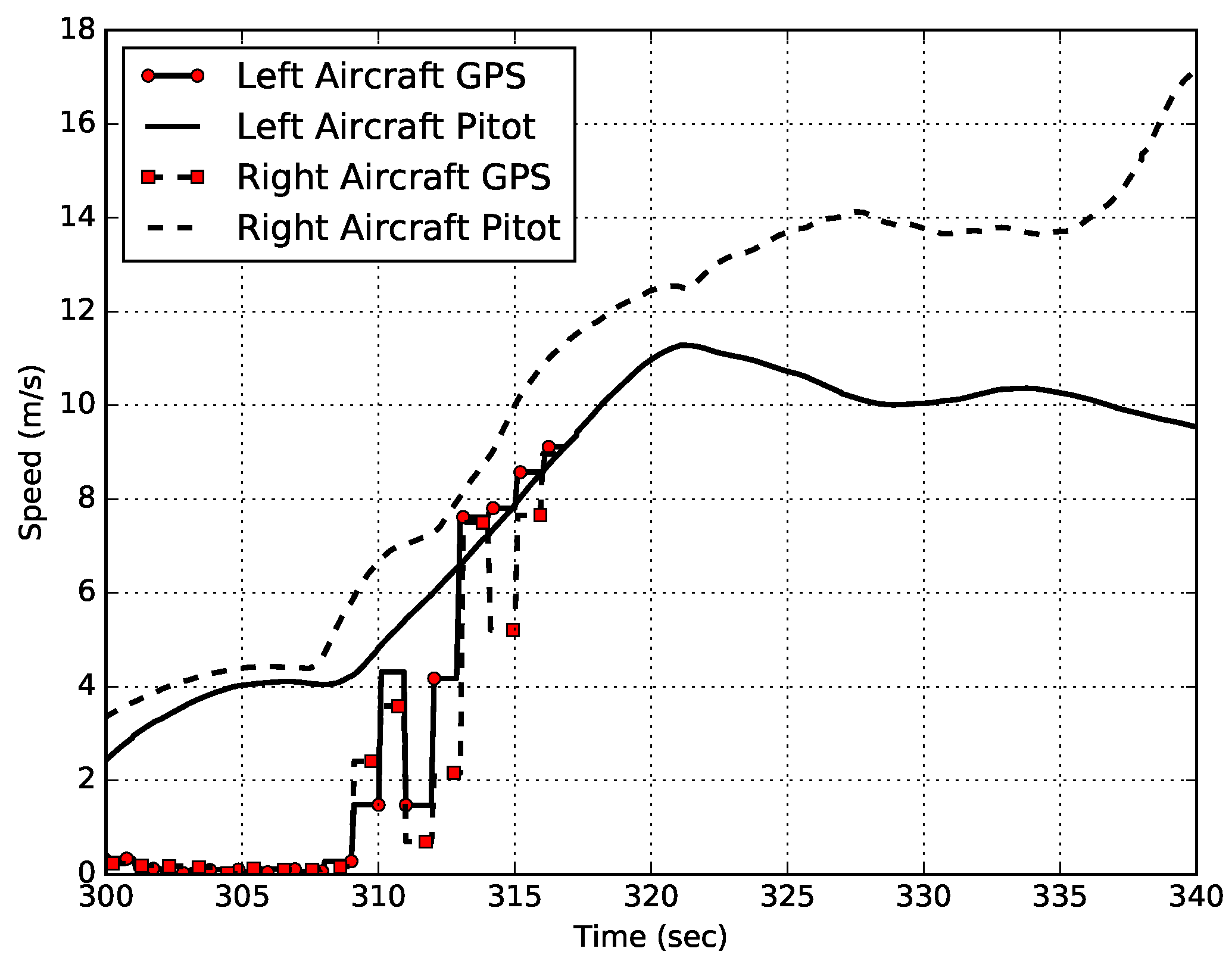
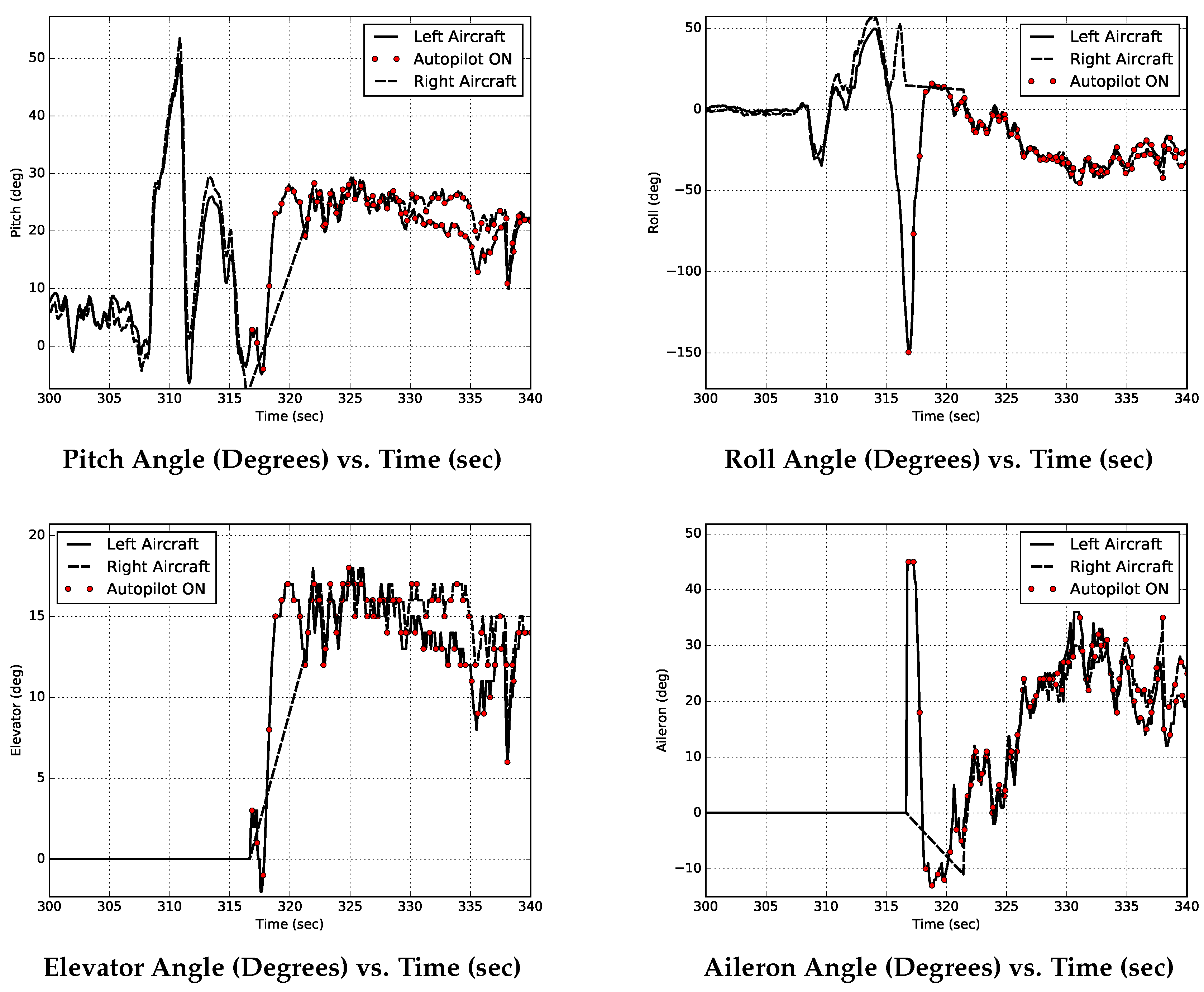
1) successfully brings the simulated aircraft to wings-level and a constant pitch angle in under 8 s. The constant pitch angle is set to 8 degrees. Experiments using one aircraft revealed that a positive 8 degree pitch angle results in an almost constant altitude at 14 m/s. These results show that the controller is capable of controlling the connected aircraft system even with a roll angle difference of up to 50 degrees. Experimental results will also highlight the issue experienced here.
6. Conclusions
The work presented here seeks to show through simulation and experiment that autonomous flight for a wing tip connected aircraft is possible and could be used as a method for increasing range and endurance. Numerous flight experiments have been conducted with many lessons learned. Simulations initially revealed that communication between aircraft is needed to achieve stable flight. Future work and simulations could focus on communication between aircraft but stable flight can still be achieved provided the aircraft has the same hardware and software and the same guidance commands, each aircraft will attain identical attitudes and achieve steady and level flight. Simulations also revealed that a priori knowledge of the configuration is not needed. That is, if a meta aircraft loses or adds an aircraft, the controller does not need to autonomously update its control laws to achieve steady and level flight. Again, provided each aircraft achieves the same roll and pitch angle, the aircraft will fly steady and level. Waypoint control however is much more complex and requires a much more sophisticated control scheme. Flight experiments presented an interesting challenge in both hardware and controls. The meta aircraft needed to be flown in a manual mode thus each receiver on the aircraft was connected to one transmitter. As shown, this presented quite an issue to fly the aircraft autonomously since any large pitch and roll deviations could not be corrected. A horizontal tailboom was added to reduce the pitch excursions but roll excursions were still experienced in flight. When these large roll deviations were experienced, the pilot was able to activate the steady and level control scheme and fly the aircraft. This proved the rather trivial result that one pilot cannot fly two aircraft at the same time and thus a meta aircraft must be flown in a semi-autonomous mode so that the aircraft attitude deviations remain small. The magnets used or the connection mechanism in general could be improved. Although the aircraft did not separate during the experiment, they did allow for large roll deviations. Perhaps a different connection mechanism could be designed to alleviate some of these deviations. In the future more simulation work must be done to simulate take offs and landings to support this semi-autonomous mode. In addition, waypoint control will also introduce an interesting problem to have both aircraft coordinate attitude control to achieve a desired heading and position. It is the recommendation of the authors to use a more robust autopilot rather than the Arduino MEGA and add landing gear to assist in landing the aircraft.


