Article

Suppression of Low-Frequency Shock Oscillations over Boundary Layers by Repetitive Laser Pulse Energy Deposition

Department of Aerospace Engineering, Nagoya University, Furo-cho, Chikusa-ku, Nagoya 464-8603, Japan
*
Author to whom correspondence should be addressed.
These authors contributed equally to this work.
Aerospace 2016, 3(2), 13; https://doi.org/10.3390/aerospace3020013
Submission received: 28 March 2016 / Revised: 18 April 2016 / Accepted: 22 April 2016 / Published: 27 April 2016
(This article belongs to the Special Issue Feature Papers in Aerospace)

Abstract

:
The effect of repetitive energy deposition on low Strouhal number oscillations of the shock wave induced by boundary-layer interaction over a cylinder-flare model was studied. The fluctuation of the energy deposition frequency was induced in the flow, because the bubble generated by the energy deposition flowed downstream along the surface repeatedly. The region before the bubble size was affected by the energy deposition directly, so the fluctuation frequency was equal to the energy deposition frequency. However, the flare shock behavior at a position farther from the surface than the bubble size was also affected strongly by the energy deposition. For low-frequency unsteadiness and the effect of energy deposition on its unsteadiness, two categories have been observed. In the relatively small flare angle case, the flare shock was oscillated owing to the fluctuation induced by the boundary-layer interaction at the shock foot, and its oscillation occurred at 2.1 kHz with a small amplitude. The amplitude of this oscillation was decreased by highly repetitive energy depositions, and its amplitude could not be detected at a highly repetitive energy deposition. In the longer cylinder section case, the region of the shock-wave interaction was widened, and the amplitude of the flare shock oscillation was increased. In this case, the amplitude drastically decreased because of energy deposition.

Graphical Abstract

1. Introduction

Shock-wave boundary-layer interaction (SWBLI) is a common phenomenon of supersonic flow. This interaction induces unsteady flow, such as boundary-layer separation or shock-wave oscillation. These unsteady flows are driven by the fluctuations in the upstream boundary layer or by the fluctuation of the shock wave, and the dominant driving mechanisms depend on the interaction strength. However, the characteristic frequency of unsteadiness in the SWBLI region is lower than other regions, such as the upstream boundary layer or downstream of the shock wave [1].
An important behaviour in shock-wave boundary-layer interactions, which is often observed in experiments, is low-frequency shock-wave oscillation. There are two possible sources of the oscillation, upstream flow fluctuation or fluctuation propagating from the downstream of the shock wave. Ganapathisubramani et al. [2,3] obtained a correlation between velocity fluctuation in the incoming flow and shock-foot motion; large-scale oscillation in the separation region had a low characteristic frequency, less than 1 kHz. Andreopoulos and Muck [4] argued that the turbulence of the incoming flow induced shock-wave oscillations. Dussauge et al. [5,6] showed that the characteristic frequencies of the incoming turbulent boundary layer was higher than that of shock motion, thereby suggesting a three-dimensional structure of the separation-bubble as the primary source of the SWBLI unsteadiness. Souverein et al. [7] concluded that high-frequency behaviour in weak interactions without separation was dominated by upstream unsteadiness, while downstream unsteadiness became predominant in strong, low-frequency interactions with separation. Although many phenomenological reports have been made, approaches to actively control the unsteadiness have not been conducted intensively.
Strategies to control SWBLI are categorized as passive or active approaches [8,9]. Passive control approaches such as cavities [10], vortex generators [11,12,13], micro-ramps [14], and strakes [15] are effective in reducing SWBLI unsteadiness; however, these approaches are effective only in limited operational condition and can cause unfavorable effects in off-design operation. Active control approaches such as energy deposition [16,17] and jet injection [18,19] can widen the effective operational ranges because the operational conditions can be tuned to the flow conditions. Impacts of the operational condition on the flow field should be investigated through parametric studies from the viewpoint of fluid dynamics. In other words, investigation of the effect of disturbances on unsteadiness in the SWBLI region can be conducted by artificially inputting flow disturbances. In past studies, it was reported that laser pulse energy deposition, which was one of the active controlling approaches, can suppress boundary-layer separation [16] or modulate the shock-wave oscillation frequencies [17]. However, little is known of the effect of the laser pulse energy deposition condition on the low-frequency unsteadiness. In [16], the suppression effect of the large-scale shock-wave oscillation is reported; however, the frequency of the oscillation has not been discussed. In [17], the low-frequency unsteadiness could not be discussed owing to the limitation of the measurement technique. Hence, the objective of this paper is to investigate the effect of the energy deposition condition on the low-frequency unsteadiness in the SWBLI region.

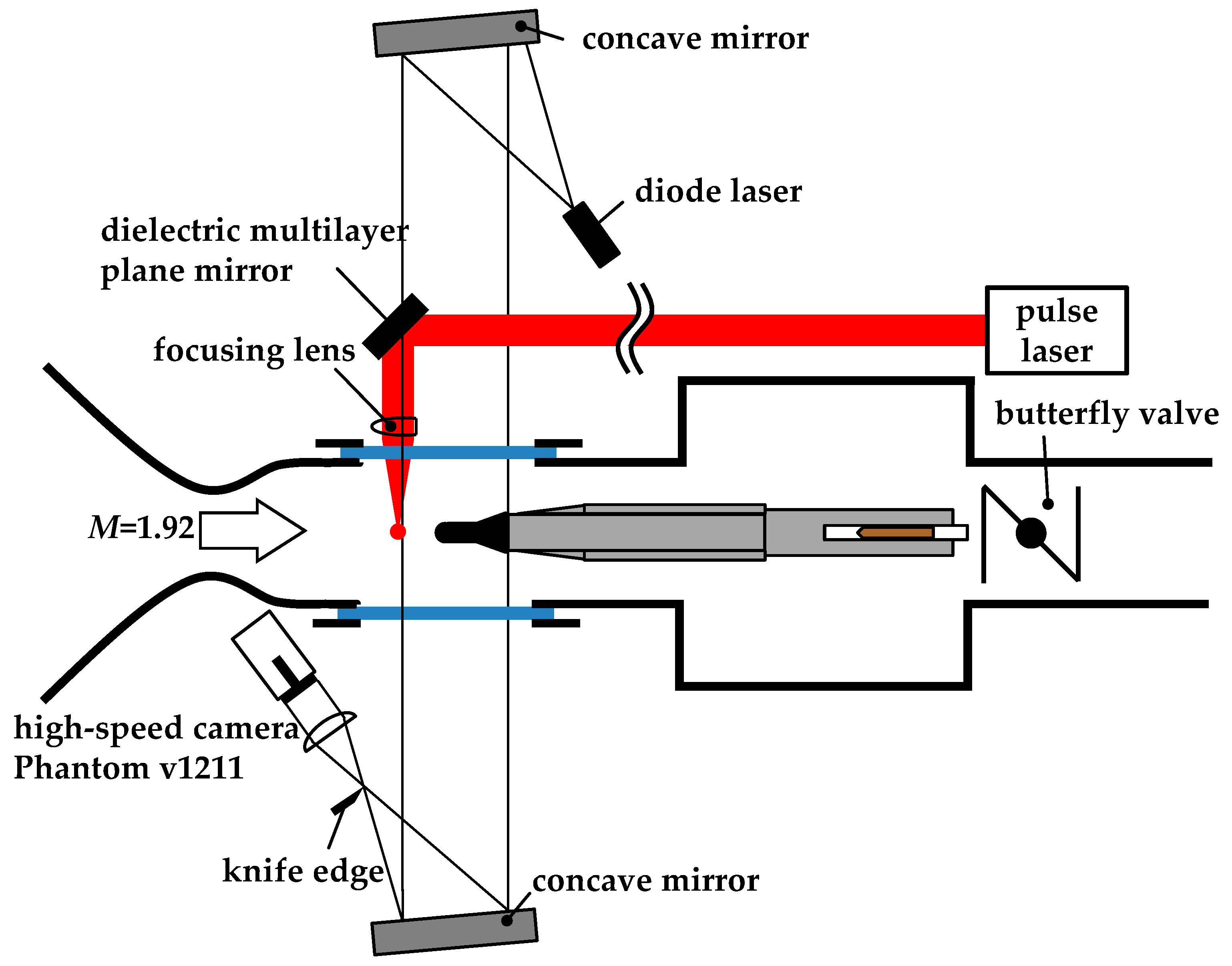
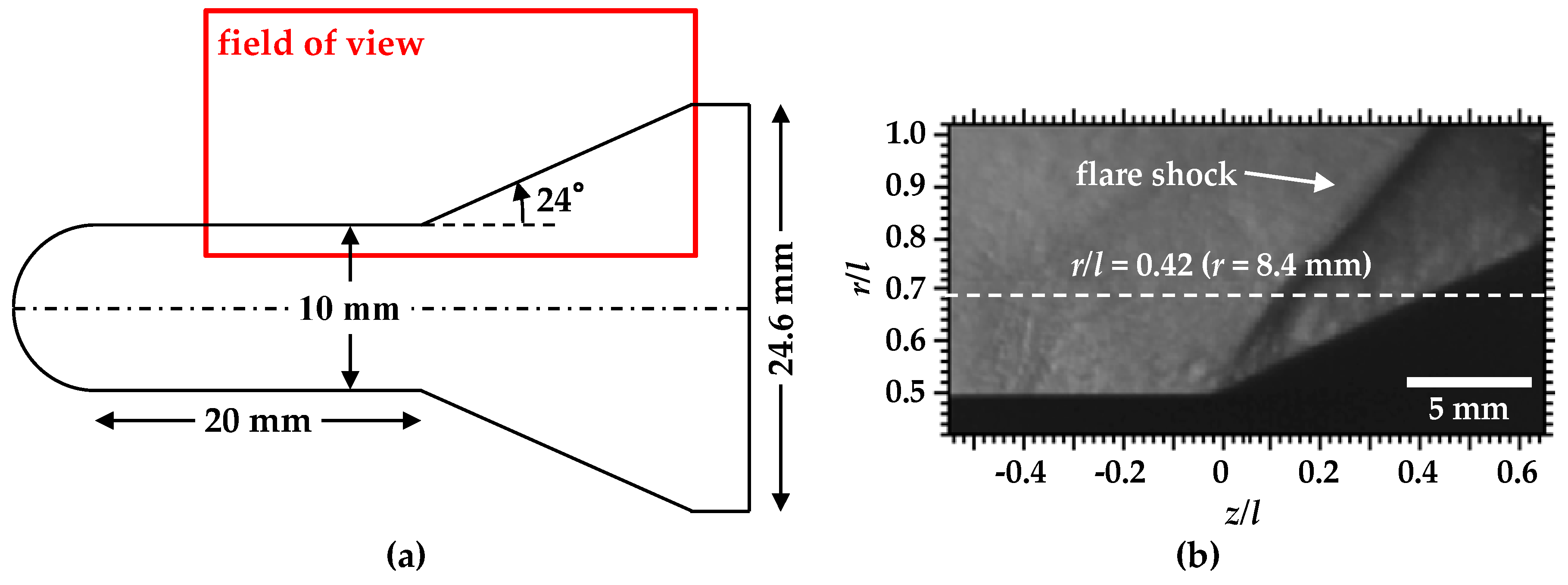
2. Experimental Apparatus and Methodology

The experiments were conducted in the in-draft supersonic wind tunnel installed at Nagoya University [16]. The schematic illustration is shown in Figure 1. The cross-sectional area of the test section was 80 mm × 80 mm. The Mach number, duration, static pressure, and static temperature of the test flow were 1.92, 3 s, 13.8 kPa, and 162 K, respectively. The test flow was visualized using the Schlieren method with a high-speed framing camera (Vision Research Inc., Wayne, NJ, USA, Phantom v1211, 1280 pixels × 800 pixels maximum, 8.2 × 10⁶ fps maximum) and a synchronized pulse diode laser (Cavitar Ltd., Tampere, Finland, CAVILUX Smart, 640 nm wavelength) through a BK7 window. Under experimental conditions, the framing rate and the image size of the camera were set to 190,476 fps and 256 pixels × 128 pixels, and the pulse duration of the light source was 10 ns. Although the minimum exposure time of the camera was 1 μs, the effective exposure time of the Schlieren image was improved by the pulse duration of the pulse diode laser. The available frame number was 2048, which was determined by the pulse number of the light source. A highly repetitive pulse laser (Nd:YVO4 laser, EdgeWave GmbH Innovative Laser Solutions, Würselen, Germany, HD40I-E, wavelength: 1064 nm, repetition frequency: up to 100 kHz, average power: up to 400 W) supplied the energy into the flow. The output laser beam with 6 mm × 6 mm square was reflected by three dielectric multilayer plane mirrors of its reflection angle of 45° after expanding to 15 mm × 15 mm square, and the expanded beam was focused at 20 mm upstream of the model through BK7 windows by using a LightPath® GRADIUM® convex lens with a focal length of 60 mm.
An axisymmetric hemisphere-cylinder-flare configuration was used for the experimental models; the configuration is shown in Figure 2 and consists of a hemispherical nose, a cylinder, and flare sections. The diameters of the hemisphere and the cylinder were 10 mm. The length of the cylinder is designated by l, and the angle of the flare by θ. The base diameter of the flare was 24.6 mm. The variables l and θ were varied as control parameters as described in Table 1. The Reynolds number defined by the upstream flow and l is 150–200. A nominal model, like the one used in [16], was the reference model. This reference model causes a completely separated boundary layer and a dispersed shock wave. The shallow model has a smaller θ, yielding a relatively weak interaction. The Long model has a larger l, thereby being accompanied by a relatively strong interaction region.
The frequency of the flare shock oscillation is determined from an 8-bit temporal brightness history of the Schlieren image using a fast Fourier transform (FFT); this is the same method as mentioned in [17]. For increasing the resolution of the frequency and the position, the field of view for frequency analysis is focused on the SWBLI region. The spatial resolution of the Schlieren images was 0.1 mm/pixel. The analysis frequency is in the range of 93 Hz to 95 kHz, which is determined by a framing rate of 190,476 fps and an effective frame number of 2048 (effective recording time of 10.75 ms). The analysis frequency range is extended by effective frame numbers; specifically, the lower frequency can be detected. The measurement uncertainty of the Strouhal number, which was determined by the product of the capability of the resolutions of the Schlieren images and the upstream flow speed of approximately 500 m/s, was 1.9 × 10⁻⁵.
The brightness history and the spectrum density against the spectrum frequency, fs, of a pixel on the shock wave, are shown in Figure 3. The temporal brightness history shown in Figure 3a is clearly oscillated at a specific frequency. This oscillation corresponds to the shock oscillation, and the frequency of this shock motion is analyzed by FFT, as shown in Figure 3b. From Figure 3b, a strong spectrum is observed at 2.4, 4.8, and 7.2 kHz. Because 4.8 and 7.2 kHz are harmonic frequencies of 2.4 kHz, the shock oscillation frequency can be considered to be 2.4 kHz. The shock oscillation frequency obtained by the brightness history corresponds to the frequency obtained by the framing images. In this way, the spectrum density against fs is obtained at each pixel, and the characteristic frequency of the shock motion can be analyzed.

3. Types of Low Frequency Oscillation and the Impact of Energy Deposition

Behaviors of SWBLI with repetitive laser pulse energy deposition were observed in the same way as described in the previous section. The repetition frequency, fe, and the pulse energy of the laser energy deposition, E, are varied in the ranges of fe = 10–80 kHz and E = 5.28–7.22 mJ/pulse, respectively. Using a laser power meter, E is evaluated by the measurement of the average power and the repetition frequency. In the laser device used in this investigation, the available laser pulse energy decreases with increasing pulse repetition frequency. The values of E for fe up to 50 kHz are set almost constant from 6.2 to 6.6 mJ/pulse, with higher values of fe as the tested value of E decreases.
Figure 4 shows the typical flow field structure of the Nominal model. Figure 4a–c show the flow field without energy deposition, and Figure 4d–f show the flow field with an energy deposition of 30 kHz. Figure 4a,d show the overall flow, Figure 4b,e show the close-up around the flare section which corresponds to the frequency analysis area, and Figure 4c,f show the close-up around the stagnation point. The low-density bubble is generated by the laser energy deposition, and the disturbance is caused by the interaction between the bubble and the bow shock, which can be seen clearly by comparing with Figure 4c,f. In Figure 4a, cylindrical coordinates (r, z) are shown. z originates at the intersection between the cylinder and the flare sections. r originates at the centreline of the model. Typically, a bow shock is formed in front of the hemisphere, the boundary layer is developed along the cylinder section, and the oblique shock, which is called a “flare shock”, is induced in front of the flare section. From Figure 4a, the flow can be considered as symmetrical, and, from Figure 4b, the boundary layer is separated, and the foot of the flare shock is not clearly visualized owing to the interaction with the boundary layer. On the other hand, in Figure 4d, the flow seems to be asymmetrical, because the energy deposition position is uncertain. However, from Figure 4e, boundary-layer separation is suppressed, and the foot of the shock wave is clearer than in Figure 4b. This modulation is the effect of the repetitive energy deposition already mentioned in [16].

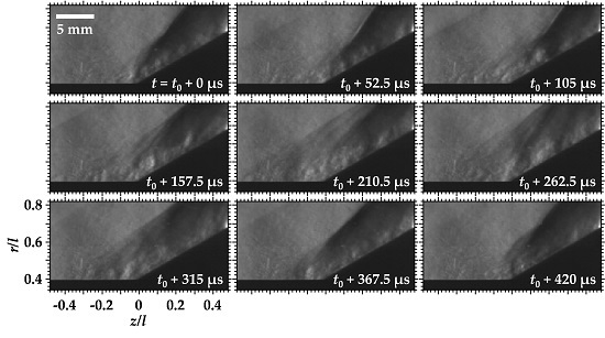
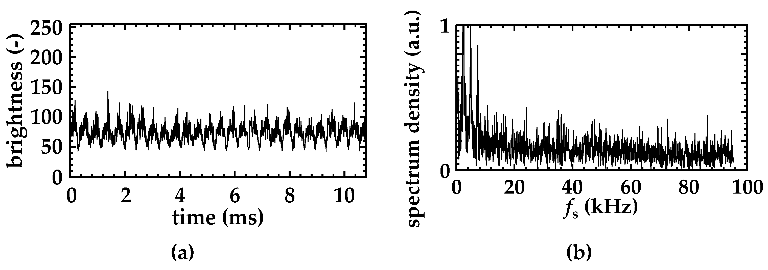
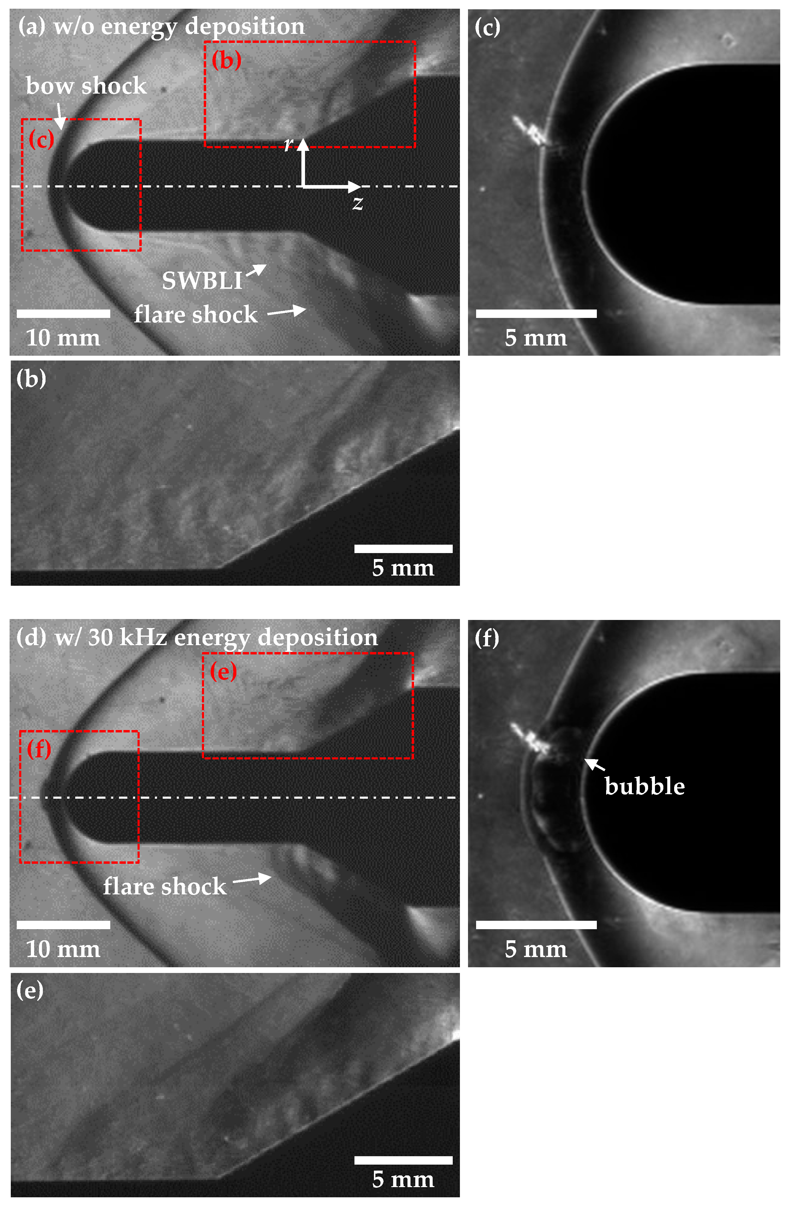
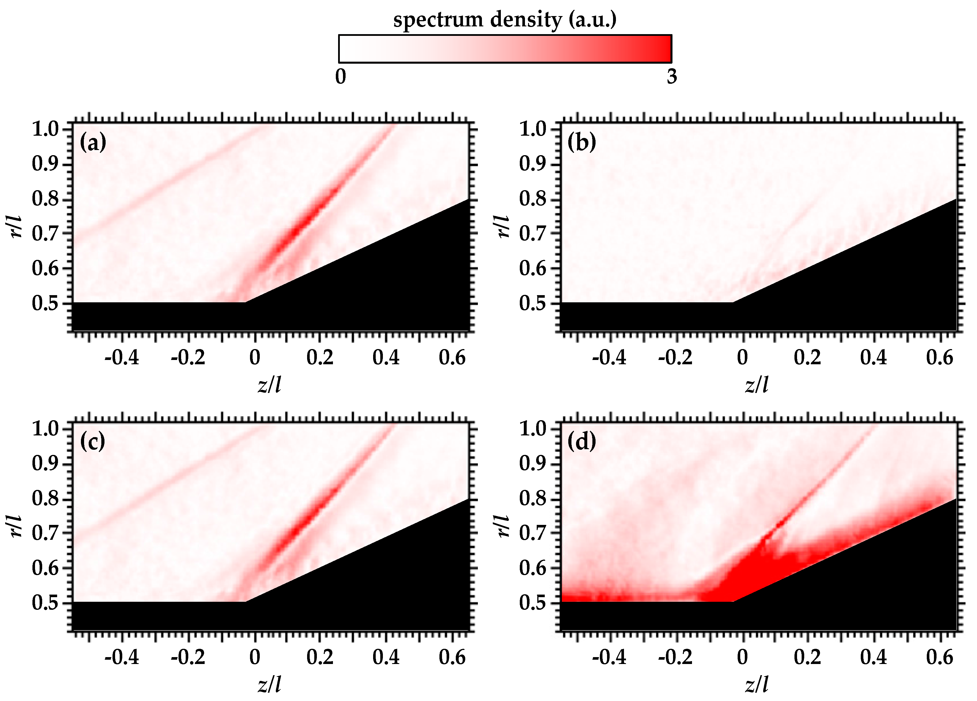
3.1. Weak Flare Fluctuation

The schematic illustration and the snapshots of the Schlieren image of the Shallow model are shown in Figure 5a,b, respectively. From Figure 5b, even though the flare shock stands in front of the flare section and serious boundary-layer separation does not occur, the flare shock oscillates owing to the fluctuation induced by the boundary-layer interaction at the shock foot. This oscillation frequency is relatively low and the oscillation amplitude is small.
Figure 6 shows the power spectrum density distribution along r/l = 0.42 (r = 8.4 mm) without and with energy deposition. The horizontal axis z corresponds to the horizontal axis of Figure 5b, and the spectrum frequency of the vertical axis corresponds to the horizontal axis of Figure 3b. The color contours correspond to the spectrum density. From Figure 6a, the Shallow model has a strong spectrum in the 1–3 kHz range owing to the flare shock fluctuation. The strongest spectrum is observed at 2.1 kHz. The amplitude of the flare shock oscillation in the z direction along r/l = 0.42 is determined from the spectrum density distribution, as shown in Figure 6. The amplitude of the Shallow model at 2.1 kHz is 1.0 mm because a strong spectrum is observed at z = 1.0–2.0 mm. The Strouhal number defined by this oscillation frequency, amplitude, and upstream flow speed of approximately 500 m/s is 4.4 × 10⁻³. From Figure 6b, in the case of fe = 40 kHz, strong spectra are observed at 30, 40, and 70 kHz. 40 kHz is the same as fe, 30 and 70 kHz are caused by the aliasing effect between the frame rate of the camera and the harmonics frequencies of 40 kHz. Hence, the strong spectrum at 40 kHz can be considered as the unique frequency induced by the aerodynamic phenomena. From this figure, the oscillation amplitude at 40 kHz is 1.4 mm, and the Strouhal number is 1.1 × 10⁻¹. As a result of the 40-kHz energy deposition, the oscillation frequency is modulated to the energy deposition frequency, and the Strouhal number increases. On the other hand, in the case of fe = 80 kHz, a strong spectrum is not observed in the flare shock region, as depicted in Figure 6c. The amplitude and the Strouhal number cannot be determined for the case of fe = 80 kHz. From these results, a highly repetitive energy deposition can suppress the flare shock oscillation induced by a weak flare fluctuation case.
Figure 7 shows the energy deposition frequency dependence of the oscillation amplitude and the Strouhal number obtained by spectra at fe = fs. The amplitude at 0 kHz corresponds to the oscillation amplitude of the strongest spectrum in the case where energy deposition was absent, fs = 2.1 kHz. For the case where the amplitude is as shown in Figure 7a, the following results were found. In the case of the Nominal model, which has a completely separated boundary layer and a dispersed shock wave, the boundary-layer separation is suppressed by the repetitive energy deposition, and a shock-wave oscillation is induced. The induced shock-wave oscillation amplitude is small, and the amplitude cannot be detected at fe ≥ 40 kHz. In the case of the Shallow model, the shock-wave oscillation is also induced by the repetitive energy depositions, and the oscillation amplitude decreases as fe increases. At repetition frequencies higher than 50 kHz, the amplitude is smaller than the natural oscillation frequency. Furthermore, the oscillation amplitude with fe ≥ 70 kHz is less than the resolution of this analysis. For the results of the Strouhal number, as shown in Figure 7b, the Strouhal number increases at fe ≤ 20 kHz and decreases at fe ≥ 20 kHz. This is caused the amplitude being the same magnitude at lower frequency conditions, but at higher frequency conditions, the amplitude is drastically decreased. At even higher repetition frequencies, the amplitude cannot be defined by this method, and the Strouhal number may decrease to less than the magnitude of the natural oscillation.

3.2. Long Interaction Region

Figure 8 shows the schematic illustration of the Long model. The flare angle of the Long model is the same as in the Nominal model, and the cylinder length is longer than in the Nominal model. In this case, the shock-wave interaction region is widened along the model surface of the cylinder section. The flare shock is oscillated at a low frequency, and the amplitude of the flare shock oscillation increases.
Figure 9 shows the snapshots of the Schlieren image. With the Long model, the flare shock and the dispersed shock are observed. In this case, the flare shock is oscillated as shown in Figure 9. The flare shock is formed at (t0 + 0) μs. This flare shock is dispersed and propagated upstream from (t0 + 52.5) to (t0 + 210.5) μs. Then, the propagated flare shock restores to the initial position from (t0 + 262.5) to (t0 + 420) μs. This motion of the flare shock is repeated with a frequency of about 2.4 kHz.
Figure 10 shows the power spectrum density distribution along r/l = 0.34 (r = 8.4 mm) without and with energy deposition. From Figure 10a, the Long model has a strong spectrum at 2.4, 4.8, and 7.2 kHz. The flare shock oscillation with the Long model is 2.4 kHz because 4.8 and 7.2 kHz are the harmonic frequencies of 2.4 kHz. This oscillation frequency is consistent with the estimated oscillation frequency by framing the Schlieren images. The amplitude of the flare shock oscillation at 2.4 kHz is 11.5 mm because a strong spectrum is observed at z = −5.9 to 5.6 mm. The Strouhal number is 5.5 × 10⁻². The oscillation frequency is similar to the Shallow model, but the Strouhal number is larger in the Long model than in the Shallow model. This difference is caused by the state of the boundary layer. The thickness of the boundary layer increases because the development length of the boundary layer of the Long model is longer than that of other models. If the boundary layer was developed enough, the large Strouhal number unsteadiness, which is mentioned in [20], occurs. From Figure 10b, the oscillation frequency is modulated to 40 kHz, and the oscillation amplitude decreases with a 40-kHz energy deposition. From Figure 10c, the oscillation frequency of fs = fe = 80 kHz was not observed, but the relative strong spectrum appeared at lower broadband frequencies.
Figure 11 shows the energy deposition frequency dependence of the oscillation amplitude and the Strouhal number obtained by spectra at fe = fs. The amplitude at 0 kHz corresponds to the oscillation amplitude of the strongest spectrum without the energy deposition case, fs = 2.4 kHz. From Figure 11a, in the case of the Long model, the magnitude of the amplitude was not strongly affected by the energy deposition at fe ≤ 20 kHz. However, the amplitude was drastically decreased when the repetition frequency was higher than 30 kHz; then, the amplitude became less than the resolution of this analysis where fe ≥ 70 kHz. For the results of the Strouhal number, as shown in Figure 11b, the tendencies were similar to the Shallow model, as shown in Figure 7b. The Strouhal number increases at fe ≤ 20 kHz and decreases at fe ≥ 20 kHz.

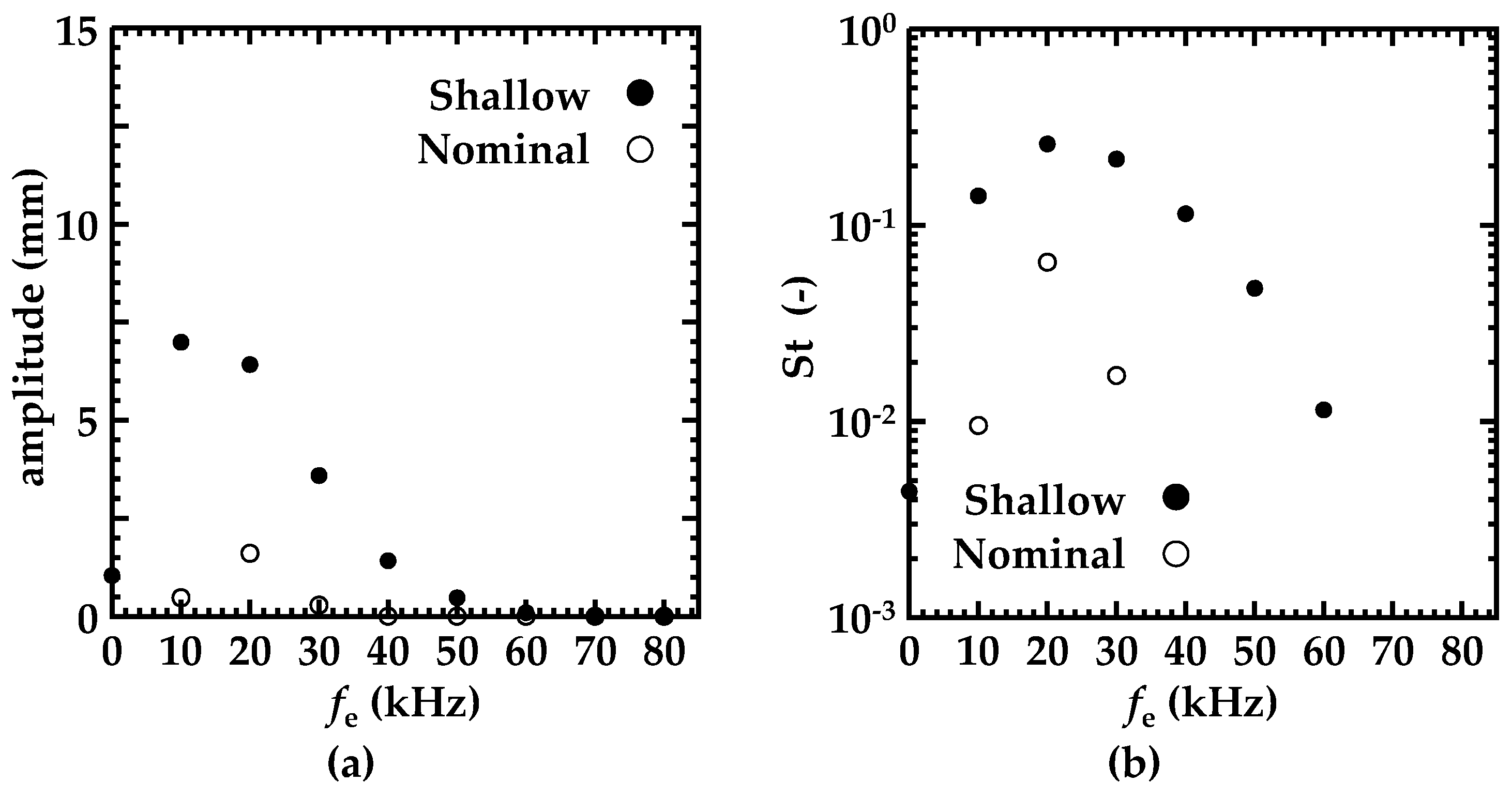
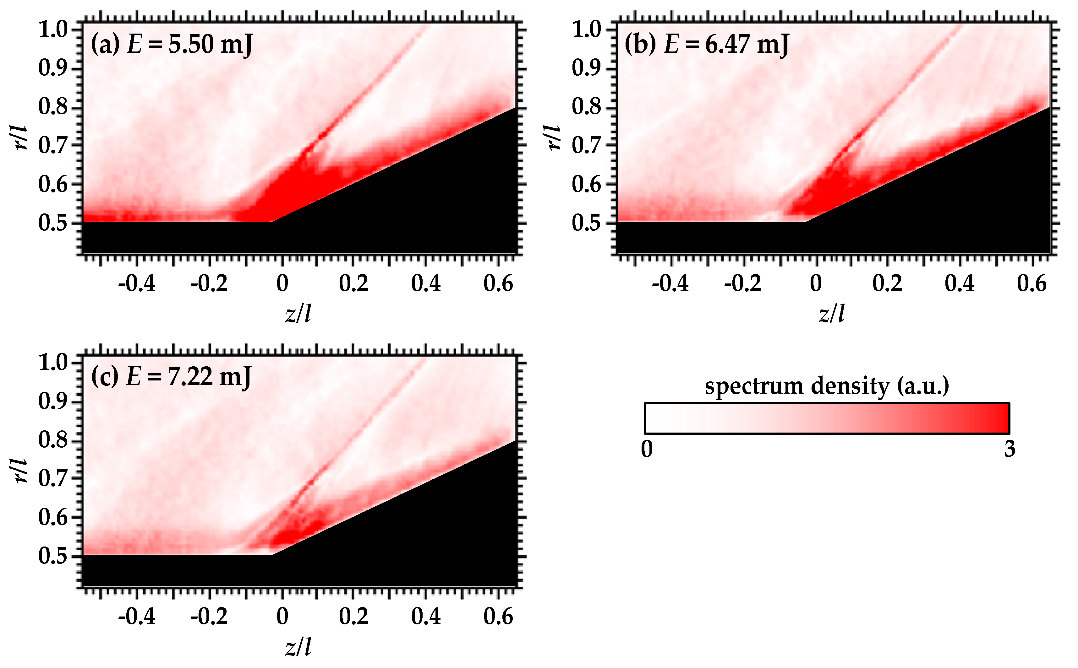
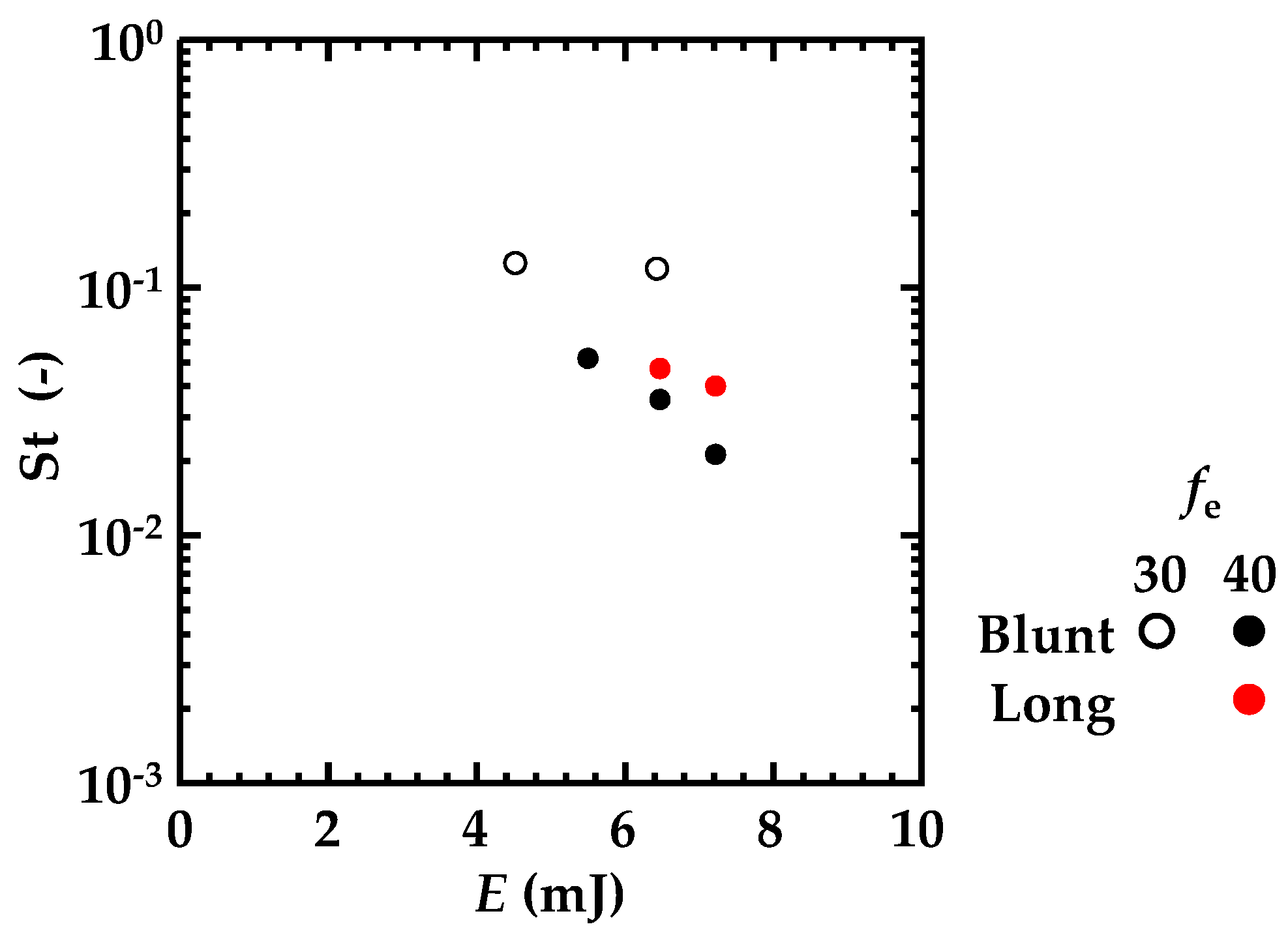
4. The Effect of Pulse Energy

The pulse energy effect was also analyzed by the same method. fe was set to 30 and 40 kHz, and the pulse energy was varied from 4.50 to 7.22 mJ/pulse. The minimum pulse energy was determined by the threshold of the laser breakdown. Figure 12 shows the spatial distributions at fs = 2.1 and 40 kHz for the Shallow model without and with a 40-kHz energy deposition. These distributions were obtained by integrating the frequency spectrum from (fs − 0.092) to (fs + 0.092) kHz. From Figure 12a,b, the case where energy deposition was absent has a strong spectrum at fs = 2.1 kHz, and no strong spectrum exists at fs = 40 kHz. On the other hand, in the fe = 40 kHz case, no strong spectrum was observed at 2.1 kHz, and the strong spectrum was observed at fs = 40 kHz. The same tendencies can apply to the case of the Long model; the case where energy deposition was absent has a strong spectrum at fs = 2.4 kHz, and the fe = 40-kHz energy deposition case has a strong spectrum at fs = 40 kHz.
Figure 13 shows the spatial distributions of the power spectrum at fs = 40 kHz for the Shallow model with fe = 40 kHz and different pulse energies. From this figure, the flare shock is oscillated at the same frequency as the energy deposition. However, the region accompanying the strong spectrum decreases as pulse energy increases. This difference is caused by the difference of the upstream disturbance supplied by the energy deposition.
Figure 14 shows the Strouhal number of the flare shock at r/l = 0.42 (r = 8.4 mm) against the pulse energy. The repetition frequencies of the energy deposition of the Shallow model are 30 and 40 kHz, and the frequency of the Long model is 40 kHz. In all experimental cases, the Strouhal number has decreasing tendencies as the pulse energy increases. The magnitude of the decrement of fe = 40 kHz is larger than that of fe = 30 kHz. The repetitive energy deposition with lower pulse energy is enough to modulate the shock-wave oscillation frequency, and the shock oscillation suppression effect of the energy deposition becomes stronger as pulse energy increases.

5. Conclusions

The repetitive pulse laser energy deposition effect on the low frequency unsteadiness induced by SWBLI was experimentally investigated. The low frequency unsteadiness of a shock wave can be classified in two categories: the low frequency unsteadiness induced by the fluctuation of the boundary-layer interaction at the shock foot and the low frequency unsteadiness induced by the widened shock-wave interaction region along the surface of the cylinder section. From the comparison of these two types of low frequency unsteadiness, the oscillation frequencies of the flare shock were similar in magnitude, but the oscillation amplitudes were different. As a result of the amplitude difference, the Strouhal number has an order of magnitude difference.
The energy deposition to the former category induced a shock oscillation with large amplitude, and the Strouhal number also increased under lower repetition frequency conditions. However, both the amplitude and the Strouhal number decreased as the frequency increased under higher repetition frequency conditions. Furthermore, under repetition frequencies of more than 70 kHz, the amplitude could not be determined, and the oscillation was completely suppressed.
The energy deposition to the latter category suppressed the amplitude of the flare shock oscillation as the repetition frequency increased, but the Strouhal number had an increasing-decreasing tendency as the frequency increased. Under repetition frequencies of more than 50 kHz, the Strouhal number was smaller than the initial magnitude, and the amplitude could not be determined for frequencies greater than 70 kHz. In addition, the results of the different pulse energies of the energy depositions showed that a higher pulse energy was more effective to suppress the amplitude of the shock-wave oscillation. Thereby, the repetitive pulse energy deposition with small pulse energy is enough to modulate the low frequency unsteadiness, and the highly repetitive pulse energy deposition or repetitive pulse energy deposition with high pulse energy can completely suppress this unsteadiness.

Supplementary Materials

Video S1: High-speed Schlieren videos of the Nominal model without energy deposition, Video S2: High-speed Schlieren videos of the Shallow model without energy deposition, Video S3: High-speed Schlieren videos of the Long model without energy deposition, Video S4: High-speed Schlieren videos of the Nominal model with 30-kHz energy deposition, Video S5: High-speed Schlieren videos of the Shallow model with 30-kHz energy deposition, Video S6: High-speed Schlieren videos of the Long model with 30-kHz energy deposition.

Acknowledgments

The authors would like to thank Messrs. Akira Saito and Masafumi Nakakimura, Technical Division, Nagoya University for their valuable technical assistance. This research was supported by the Japan Society for Promotion of Science, Grant-in-Aid for Scientific Research (A), No. 15H02321.

Author Contributions

Akihiro Sasoh conceived and designed the experiments. Akira Iwakawa, Tatsuro Shoda, and Hoang Son Pham conducted the experiments. Akira Iwakawa, Tatsuro Shoda, and Takahiro Tamba analysed the experimental data. Akira Iwakawa wrote the paper.

Conflicts of Interest

The authors declare no conflict of interest.

Abbreviations

SWBLI
Shock-wave boundary-layer interaction

References

  1. Clemens, N.T.; Narayanaswamy, V. Low-Frequency Unsteadiness of Shock Wave/Turbulent Boundary Layer Interactions. Annu. Rev. Fluid Mech. 2014, 46, 469–492. [Google Scholar] [CrossRef]
  2. Ganapathisubramani, B.; Clemens, N.T.; Dolling, D.S. Effects of upstream boundary layer on the unsteadiness of shock-induced separation. J. Fluid Mech. 2007, 585, 369–394. [Google Scholar] [CrossRef]
  3. Ganapathisubramani, B.; Clemens, N.T.; Dolling, D.S.; Road, P.C. Low-frequency dynamics of shock-induced separation in a compression ramp interaction. J. Fluid Mech. 2009, 636, 397–425. [Google Scholar] [CrossRef]
  4. Andreopoulos, J.; Muck, K.C. Some new aspects of the shock-wave/boundary-layer interaction in compression-ramp flows. J. Fluid Mech. 1987, 180, 405. [Google Scholar] [CrossRef]
  5. Dussauge, J.-P.; Dupont, P.; Debieve, J.-F. Unsteadiness in shock wave boundary layer interactions with separation. Aerosp. Sci. Technol. 2006, 10, 85–91. [Google Scholar] [CrossRef]
  6. Dussauge, J.P.; Piponniau, S. Shock/boundary-layer interactions: Possible sources of unsteadiness. J. Fluids Struct. 2008, 24, 1166–1175. [Google Scholar] [CrossRef]
  7. Souverein, L.J.; Dupont, P.; Debiève, J.-F.; van Oudheusden, B.W.; Scarano, F.; Debieve, J.-F.; van Oudheusden, B.W.; Scarano, F. Effect of Interaction Strength on Unsteadiness in Shock-Wave-Induced Separations. AIAA J. 2010, 48, 1480–1493. [Google Scholar] [CrossRef]
  8. Panaras, A.G. Review of the physics of swept-shock/boundary layer interactions. Prog. Aerosp. Sci. 1996, 32, 173–244. [Google Scholar] [CrossRef]
  9. Dolling, D.S. Fifty years of shock-wave/boundary-layer interaction research: What next? AIAA J. 2001, 39, 1517–1531. [Google Scholar] [CrossRef]
  10. McCormick, D.C. Shock/boundary-layer interaction control with vortex generators and passive cavity. AIAA J. 1993, 31, 91–96. [Google Scholar] [CrossRef]
  11. Barter, J.W.; Dolling, D.S. Reduction of fluctuating pressure loads in shock/boundary-layer interactions using vortex generators. AIAA J. 1995, 33, 1842–1849. [Google Scholar] [CrossRef]
  12. Barter, J.W.; Dolling, D.S. Reduction of fluctuating pressure loads in shock/boundary-layer interactions using vortex generators. II. AIAA J. 1996, 34, 195–197. [Google Scholar] [CrossRef]
  13. Titchener, N.; Babinsky, H. Shock Wave/Boundary-Layer Interaction Control Using a Combination of Vortex Generators and Bleed. AIAA J. 2013, 51, 1221–1233. [Google Scholar] [CrossRef]
  14. Saad, M.R.; Zare-Behtash, H.; Che-Idris, A.; Kontis, K. Micro-ramps for hypersonic flow control. Micromachines 2012, 3, 364–378. [Google Scholar] [CrossRef]
  15. Kontis, K. Flow control effectiveness of jets, strakes, and flares at hypersonic speeds. Proc. Inst. Mech. Eng. Part G J. Aerosp. Eng. 2008, 222, 585–603. [Google Scholar] [CrossRef]
  16. Osuka, T.; Erdem, E.; Hasegawa, N.; Majima, R.; Tamba, T.; Yokota, S.; Sasoh, A.; Kontis, K. Laser energy deposition effectiveness on shock-wave boundary-layer interactions over cylinder-flare combinations. Phys. Fluids 2014, 26, 096103. [Google Scholar] [CrossRef]
  17. Tamba, T.; Pham, H.S.; Shoda, T.; Iwakawa, A.; Sasoh, A. Frequency modulation in shock wave-boundary layer interaction by repetitive-pulse laser energy deposition. Phys. Fluids 2015, 27, 091704. [Google Scholar] [CrossRef]
  18. Kontis, K. Jet Control Effectiveness Studies on a Flat-Plate Body at Hypersonic Speeds. Trans. Jpn. Soc. Aero. Space Sci. 2004, 47, 131–137. [Google Scholar] [CrossRef]
  19. Erdem, E.; Kontis, K. Numerical and experimental investigation of transverse injection flows. Shock Waves 2010, 20, 103–118. [Google Scholar] [CrossRef]
  20. Feszty, D.; Badcock, K.J.; Richards, B.E. Driving Mechanisms of High-Speed Unsteady Spiked Body Flows, Part 1: Pulsation Mode. AIAA J. 2004, 42, 95–106. [Google Scholar] [CrossRef]
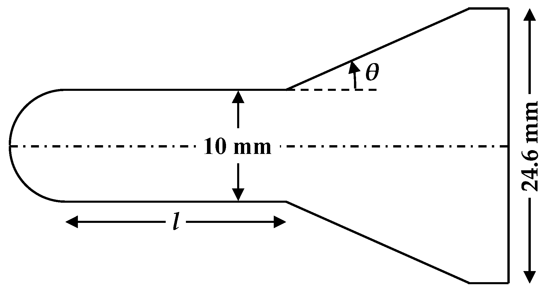
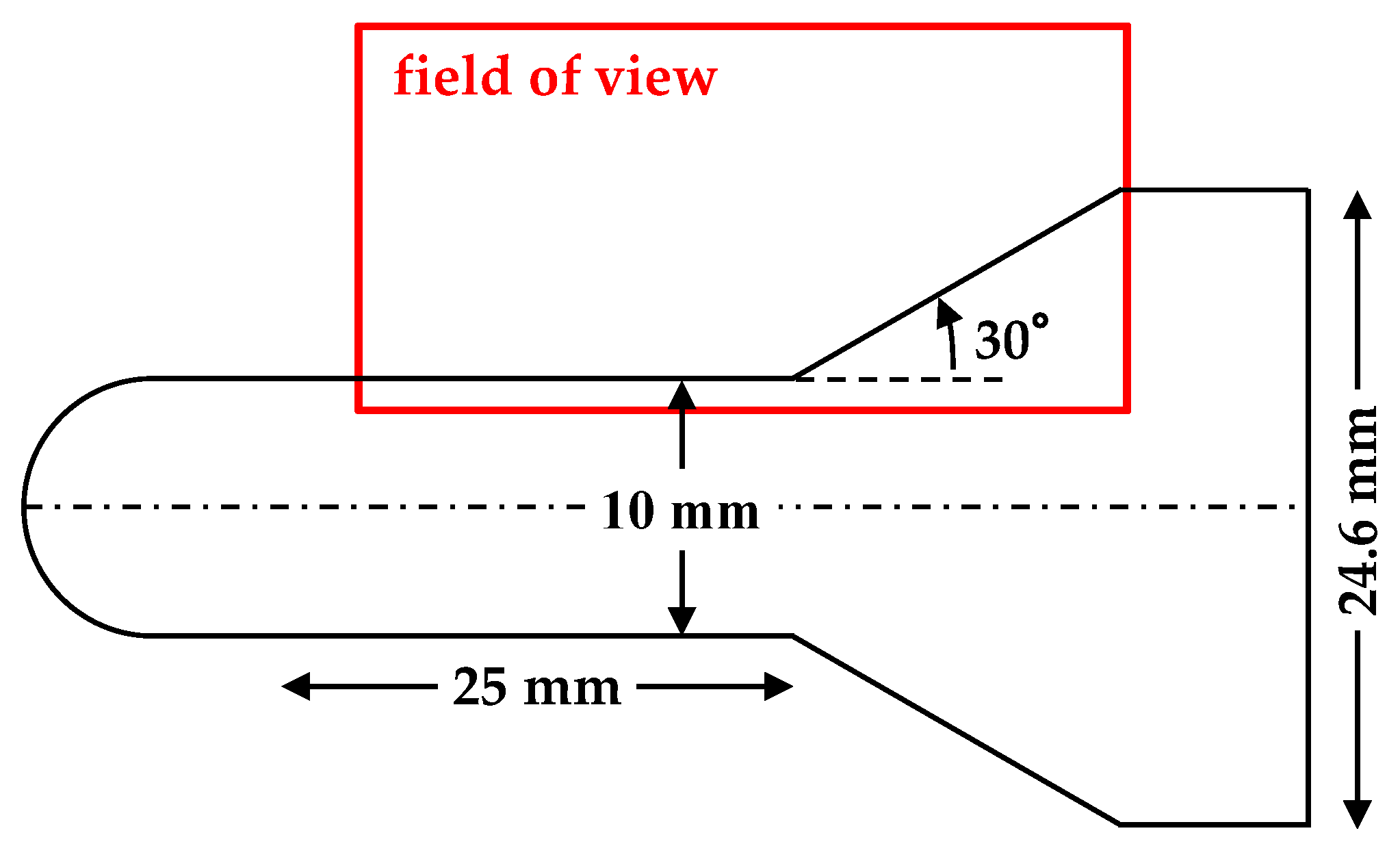
Figure 1. Schematic illustration of the experimental apparatus.
Aerospace 03 00013 g001
Figure 2. Hemisphere-cylinder-flare Long model configuration.
Aerospace 03 00013 g002
Figure 3. Frequency analysis results of a pixel of the Long model: (a) brightness history; (b) spectrum density against spectrum frequency.
Aerospace 03 00013 g003
Figure 4. Typical flow structure of the Nominal model obtained by framing the Schlieren image: (a) without energy deposition; (b) close-up around the flare section without energy deposition; (c) close-up around the stagnation point without energy deposition; (d) fe = 30 kHz; (e) close-up around the flare section with fe = 30 kHz; (f) close-up around the stagnation point with fe = 30 kHz.
Aerospace 03 00013 g004
Figure 5. Schematic illustration and snapshot of the Schlieren image of the Shallow model: (a) Schematic illustration; (b) Snapshot of the Schlieren image.
Aerospace 03 00013 g005
Figure 6. Distributions of power spectrum density along r/l = 0.42 of the Shallow model: (a) without energy deposition; (b) fe = 40 kHz; (c) fe = 80 kHz.
Aerospace 03 00013 g006
Figure 7. Oscillation amplitude and Strouhal number of the Shallow model with fe along r/l = 0.42: (a) Oscillation amplitude; (b) Strouhal number.
Aerospace 03 00013 g007
Figure 8. Schematic illustration of the Long model.
Aerospace 03 00013 g008
Figure 9. Framing Schlieren images of the Long model.
Aerospace 03 00013 g009
Figure 10. Distributions of power spectrum density along r/l = 0.34 for the Long model: (a) without energy deposition; (b) fe = 40 kHz; (c) fe = 80 kHz.
Aerospace 03 00013 g010
Figure 11. Oscillation amplitude and Strouhal number of the Long model with fe, along r/l = 0.34: (a) Oscillation amplitude; (b) Strouhal number.
Aerospace 03 00013 g011
Figure 12. Spatial distributions of the spectrum of the Shallow model: (a) fs = 2.1 kHz without energy deposition; (b) fs = 40 kHz without energy deposition; (c) fs = 2.1 kHz with energy deposition of fe = 40 kHz, E = 5.50 mJ/pulse; (d) fs = 40 kHz with energy deposition of fe = 40 kHz, E = 5.50 mJ/pulse.
Aerospace 03 00013 g012
Figure 13. Spatial distributions of the spectrum of fs = 40 kHz: (a) fe = 40 kHz, E = 5.50 mJ/pulse; (b) fe = 40 kHz, E = 6.47 mJ/pulse; (c) fe = 40 kHz, E = 7.22 mJ/pulse.
Aerospace 03 00013 g013
Figure 14. Strouhal number against the pulse energy of fe = 30 and 40 kHz.
Aerospace 03 00013 g014
Table 1. Parameters of experimental models.
Typel (mm)θ (°)
Nominal2030
Shallow2024
Long2530

