Article

Nonintrusive Aerodynamic Shape Optimisation with a POD-DEIM Based Trust Region Method

1
School of Mechanical Engineering Sciences, The University of Surrey, Guildford GU2 7XH, UK
2
School of Mechanical and Aerospace Engineering, Queen’s University Belfast, Belfast BT9 5AH, UK
3
Department of Computing, Engineering and Media, De Montfort University, Leicester LE1 9BH, UK
*
Author to whom correspondence should be addressed.
These authors contributed equally to this work.
Aerospace 2023, 10(5), 470; https://doi.org/10.3390/aerospace10050470
Submission received: 6 March 2023 / Revised: 12 May 2023 / Accepted: 15 May 2023 / Published: 17 May 2023
(This article belongs to the Section Aeronautics)

Abstract

:
This work presents a strategy to build reduced-order models suitable for aerodynamic shape optimisation, resulting in a multifidelity optimisation framework. A reduced-order model (ROM) based on a discrete empirical interpolation (DEIM) method is employed in lieu of computational fluid dynamics (CFD) solvers for fast, nonlinear, aerodynamic modelling. The DEIM builds a set of interpolation points that allows it to reconstruct the flow fields from sets of basis obtained by proper orthogonal decomposition of a matrix of snapshots. The aerodynamic reduced-order model is completed by introducing a nonlinear mapping function between surface deformation and the DEIM interpolation points. The optimisation problem is managed by a trust region algorithm linking the multiple-fidelity solvers, with each subproblem solved using a gradient-based algorithm. The design space is initially restricted; as the optimisation trajectory evolves, new samples enrich the ROM. The proposed methodology is evaluated using a series of transonic viscous test cases based on wing configurations. Results show that for cases with a moderate number of design variables, the approach proposed is competitive with state-of-the-art gradient-based methods; in addition, the use of trust region methodology mitigates the likelihood of the optimiser converging to, shallower, local minima.

1. Introduction

The pressure to reduce design cycles, increase performance or further explore design spaces keeps on demanding more efficient analysis tools. Typical engineering problems, such as aerodynamic shape optimisation, require sophisticated analysis tools to solve parametric partial differential equations (PDEs). This is a challenging process due to the high computational cost associated with having to interrogate a large and complex model multiple times. The advent of adjoint methods to compute gradients at a cost independent of the number of design variables opened up the perspective of affordable design whilst retaining a high-fidelity model [1,2,3,4,5,6]. The solution of the CFD adjoint equations requires similar computational resources to those used to solve the original flow equations. Furthermore, adjoint methods require the modification of the original software code, which may or may not be available to users. Therefore, the use of high-fidelity models in design optimisation is feasible, but not necessarily trivial or affordable.
Several strategies are available to accelerate the time to solution required for a given analysis, in particular for problems such as optimisation or uncertainty quantification, where it is necessary to interrogate a large and complex model multiple times. One common approach is to build surrogate models and devise a multifidelity strategy to compute the quantity of interest efficiently. Surrogates are typically based on interpolation methods such as response surfaces or kriging [7,8,9,10] or neural networks [11,12]; it is also possible to resort to lower-fidelity models that remain representative of some relevant physical phenomenon to act as an effective surrogate [13,14]. The obvious penalty of such strategies is on how to guarantee that the method converges to a local optimum common with the high-fidelity model; in addition, users face challenges in associating models and respective parameterisations that use very different representations of the same problem.
A slightly different alternative is to build a ROM by examining the governing equations and performing some type of model reduction that is suitable for the physics of the problem. Here, the common approach is to assume that the parametric behaviour of the high-fidelity model can be approximated by a small number of modes or basis, typically obtained by methods such as proper orthogonal decomposition (POD) [15], balance POD [16,17] or proper generalised decomposition [18], among others—extensive reviews on the wider subject of model reduction can be found in [19,20,21,22,23,24]. The exploitation of ROMs for aerodynamic shape optimisation was investigated by LeGresley and Alonso [25] for inverse aerofoil design, where a POD ROM was used to approximate the gradient of the objective function by finite differencing. Investigators have also been successful in deriving efficient ROMs for shape optimisation problems described by elliptical PDEs, such as those found in marine or biological applications [26,27,28]. The problem of aerofoil shape optimisation subject to compressible flows was revisited by Zahr and Farhat; the authors assumed a monotonic nonlinear trust region optimisation method that updates the reduced basis as the optimisation progresses when the residual fails to reach a required threshold [29]. Carlberg et al. exploit a least-squares Petrov–Galerkin projection [30] to reduce the state equations and respective sensitivities; hence, each snapshot involved concatenating samples of the fluid-state variables and sensitivities with respect to the design variables. Yao et al. employed a similar strategy, but for gradient-based optimisation for aerofoils in compressible and transonic flows, reducing the time to solution by 30–50% with respect to an adjoint-based optimisation [31].
One particular challenge with the aforementioned ROM strategies is that they are intrusive, i.e., they require the manipulation of the original CFD solver, which may not be available or desirable. In reference [32], the authors investigate the ability of the DEIM [33] of reconstructing unsteady flowfields for the prediction of dynamic aeroelastic instabilities. Inspired by these findings, and to overcome the difficulties of intrusive methods whilst obtaining high computational efficiency, this paper proposes a nonintrusive strategy suitable for aerodynamic shape optimisation; this is achieved by a new nonlinear mapping between the surface DEIM points and flow quantities of interest, allowing the DEIM ROM to reconstruct surface flow fields for new shapes. The paper will also show how a trust region model management (TRMM) ROM is able to drive the aerodynamic shape to new local minima at a reduced cost with respect to adjoint-based optimisation, while treating the high-fidelity model as a black box.
The remainder of the paper provides details of the DEIM formulation and the TRMM algorithm. This is followed by the description and analysis of two transonic, viscous wing test cases. The paper is completed with a conclusion section.

2. Methodology

2.1. The General Optimisation Problem

A constrained aerodynamic shape optimisation can be represented by [31]
minimise μ D F ( w ( μ ) , μ ) subject to R ( w ( μ ) , μ ) = 0 , C E ( w ( μ ) , μ ) = 0 , C I ( w ( μ ) , μ ) 0 .
In Equation (1), the objective function F depends on the flow variables w = [ ρ , ρ U , ρ E ] and parameter set μ . Typically, F denotes an aerodynamic coefficient such as C L or C D ; therefore, the nonintrusive ROM aims to reconstruct the surface pressure and wall shear stress fields to compute the required aerodynamic coefficients. This leads to a data-driven ROM, based on samples of the aforementioned quantities from the CFD full-order model (FOM), which are reduced by POD and a DEIM algorithm; this allows the flow field of every new shape produced by the optimiser to be reconstructed. The parameter set μ represents the design variables manipulated by the optimiser to control the aerodynamic shape. The different components required are outlined are described in the following sections.

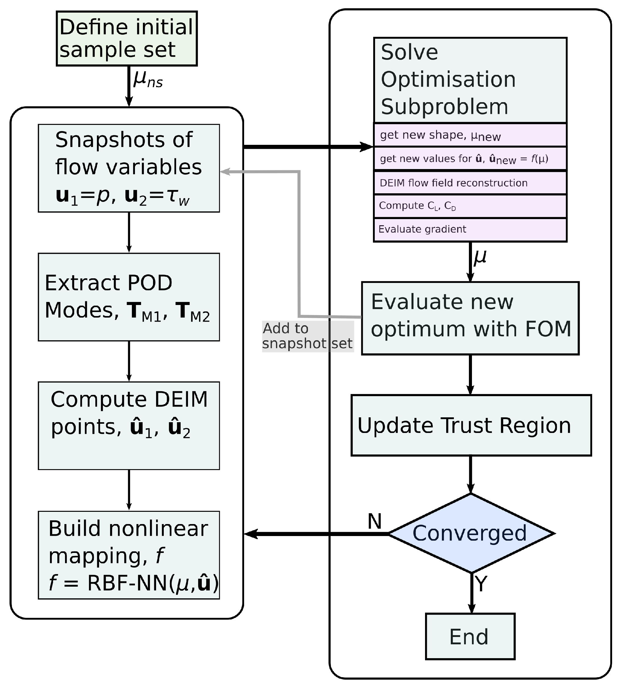
2.2. Nonintrusive Reduced-Order Modelling

The DEIM aims to approximate u as a nonlinear function of μ , where u = u ( w , μ ) , by projecting it on the subspace spanned by the basis T M :
u ( μ ) T M c ( μ ) ,
where c ( μ ) represents a set of coefficients and the matrix T M is obtained by POD of flow snapshots of the quantities represented by u , which can be p, τ w , etc. The task now is how to select the M distinct rows or interpolation indices that allow a unique solution of c ( μ ) to be obtained. This can be achieved by following the algorithm in [33]; the interpolation indices are coded into the matrix , which can be obtained using Algorithm 1, and the result is the DEIM approximation:
u ( μ ) T M T T M 1 T u ^ ( μ ) .
Algorithm 1 DEIM method for interpolation index selection [33]
 Input: Subspace T M R N × n r
 Output: Interpolation indices = [ 1 , , n r ] T
1:
[ i m a x , 1 ] = [ a r g m a x ( T 1 ) a , m a x ( | T 1 | ) ]
2:
for  i = 2 to n r  do
3:
    X = T ( : , i ) ;
4:
   solve ( T T ) c ( μ ) = T X for c ( μ ) ;
5:
    r = X T c ( μ ) ;
6:
    [ i m a x , i ] = [ a r g m a x ( r ) , m a x ( | r | ) ] ;
7:
    = [ , i ] T ;
8:
end for
For cases such as those presented here, the objective function is obtained through integrating the fluid forces over surfaces; hence, the size of the ROM can be further reduced by letting u ^ ( μ ) represent only the values of the surface pressure and shear stress corresponding to the nonzero indices in , i.e., the M elements required to recover the full-order vector u ( μ ) .
Thus, for viscous problems, the pressure and each component of the wall shear stress are individually reconstructed using Equation (3) and a respective set of bases, T M .

2.3. Proper Orthogonal Decomposition

The basis T M can be built by taking the POD modes of the flow field. This requires obtaining a set of snapshots and assembling the matrix A , where each column represents the flow solution vector for one particular set of parameter values μ :
A = u 1 , u 2 , , u n s ,
where n s is the number of samples. Since n s is much smaller than the dimension of u , the POD modes can be obtained by performing singular value decomposition (SVD) to A T A , where A T A R n s × n s :
A T A = T S V T ,
where S is a diagonal matrix containing the eigenvalues and T , V are the left and right singular vectors, respectively. The POD bases, T M R n s × N , are obtained with proper truncation according to the energy rank given by the amplitude of the first M eigenvalues:
T M = A V M S M 1 / 2

2.4. Interpolation Point Estimation

To employ the DEIM in lieu of a high-fidelity model, it is necessary to obtain u ^ ( μ ) for any shape produced by the optimiser. In this work, a nonlinear mapping between the design parameters μ and the flow values at the interpolation indices needs to be built. Note that μ and u ^ are vectors of distinct sizes, which results in a multi−input/multi−output problem. Any suitable interpolation method can be used here; following from reference [32], an exact radial basis function (RBF) neural network using the MatLab function newrbe [34] was built using the respective input/output sample pairs ( μ i , u ^ i ) , i = 1 , , n s . This interpolation method ensures that the function values interpolated are exact at the sample points.

2.5. Trust Region Model Management

Obtaining a set of global bases is usually not achievable, or would require and excessive number of snapshots, rendering the ROM approach unattractive. An alternative is to start with a small number of samples and augment the snapshot matrix as the optimisation progresses, as demonstrated in [29,31]. Trust region methods are provable to be convergent and able to manage the exchanges between different fidelity models. At each major iteration k, an optimisation subproblem is defined on the trust region centred at μ k and radius Δ k :
minimise s B k F ^ ( u ( μ k ) , μ ) subject to C ^ E ( u ( μ k ) , μ k + s ) = 0 , C ^ I ( u ( μ k ) , μ k + s ) 0 , l b ( μ k + s ) u b , | | s | | Δ k ,
where the “ ^ ” symbol indicates quantities computed using Equation (3); s is the optimisation step size; and B k = { μ R n p : | | μ μ k | | Δ k } . The optimisation subproblem was solved using MatLab’s fmincon with the gradients obtained by finite differences using the DEIM ROM.
The effectiveness of the trust region step is evaluated by the ratio of the actual improvement over the improvement predicted by the ROM, ρ :
ρ k = Δ F Δ F ^ ,
where Δ F = F ( μ k ) F ( μ k + s ) and Δ F ^ = F ^ ( μ k ) F ^ ( μ k + s ) . The step is accepted, except if Δ F is nonpositive. In addition, for values of ρ < δ 1 or ρ > δ 2 , the trust region radius is maintained if Δ F > 0 , and decreased if Δ F 0 ; if δ 1 < ρ < δ 2 , the trust region size is increased. In this work, the trust region is set up with δ 1 = 0.80 and δ 2 = 1.20 ; the trust region size, Δ k + 1 , is then reduced by a factor of 0.75 , maintained or increased by a factor 1.25 . Numerical experiments show these values to perform adequately over a range of test cases. The sequence of steps is outlined in Figure 1.

3. Results

The framework described was demonstrated using two wing test cases and different drag minimisation problems. The first test case involved the Onera M6 wing, test 2308, as described in [35]. This is a widely used test case by the CFD community [36]; hence, it acts as the first benchmark for the method proposed in this work. The second test case employed the NASA Common Research Model (CRM) wing [37]. The FOMs were built using the S U 2 software v7.07 [38]; in all cases, the compressible RANS equations were solved employing the Spallart–Almaras turbulence model; the full details of the flow equation descriptions and implementation, including the turbulence model, are given in reference [38].

3.1. Onera M6 Test Case

A baseline mesh for the optimisation study was selected following the grid convergence results shown in Figure 2. This study was performed at M = 0.84 , R e y n o l d s n . = 11.7 × 10 6 and α = 3.06 ° . The meshes included a fine mesh containing about 2.2 million elements, a medium mesh with approximately 315 thousand cells and a coarse mesh made up with approximately 140 thousand elements. The medium mesh, shown in Figure 3a, was selected for the baseline optimisation case as it gives adequate results without demanding excessive computational resources (mesh obtained from: https://github.com/su2code/TestCases/tree/master/optimization_rans/steady_oneram—accessed on 3 June 2022).
The wing is parameterised using 60 control points equally distributed over the top and lower surfaces of the wing. The surface mesh shape is controlled by the position of the control points and deformed by an RBF morphing method [39]. The surface mesh and associated control points are illustrated in Figure 3b.
To build the ROM, four quantities are required from the FOM: pressure, and three Cartesian components of the shear stress projected on the surface mesh. Each quantity is used to build a set of bases and interpolation point matrix, ; therefore, each function evaluation using the ROM requires reconstructing a matrix with ( N S u r f × 4 ) elements. The reconstruction of the surface values at the sample points was exact; as an example, considering the test case conditions described above, Figure 4a–c shows two samples and resultant DEIM points (the DEIM points locations are highlighted by the black markers), the C p ROM values are plotted against the FOM results for each respective sample in Figure 4b–d, illustrating the exact reconstruction of the surface field.
The result of applying the ROM built from these two samples to a new wing shape is compared in Figure 5. As expected, the ROM predictions degraded. The level of degradation was mitigated by controlling the trust region radius. This shows that in principle, an optimisation problem can be initiated with any number of samples, including a single point; however, numerical experiments show that this is inefficient, as due to the low accuracy during the initial steps, 5−10 initial samples tend to produce faster convergences.
To facilitate benchmarking, the optimisation problem set up targets the wing at M = 0.84 , R e y n o l d s n . = 11.7 × 10 6 and α = 3.06 ° , and aims to minimise C D whilst maintaining the C L above or on the value corresponding to the baseline wing:
minimise μ D C D subject to C L > 0.25 ,
where μ defines the control point positions that manipulate the wing shape.
The ROM at the start of the optimisation was built with ten snapshots. The problem was run on 4 Intel Core 5 CPUs, with both FOM and fmincon gradient calculations running in parallel. Note that the gradients were obtained by finite differences using the ROM; this operation scales linearly with the number of CPUs available. The optimisation convergence is shown in Figure 6, where both constraint and objective functions are normalised with respect to the baseline values for C D and C L , which are 0.018 and 0.25, respectively. The right vertical axis shows the normalised value of the trust region radius, Δ , with respect to its initial value; the convergence is plotted against the total number of FOM calls, i.e., the number of trust region updates plus the FOM calls used to build the initial ROM. The cost of the ROM calls is about 10 % of a single FOM evaluation, per trust region iteration; this cost scales with the number of design variables, but is also dependent on the convergence of each optimisation subproblem.
The solution terminates after 150 iterations and results in a drag reduction of about 36 % . Note that the trust region radius increases significantly as new snapshots enrich the POD basis, meaning that a larger portion of the design space is explored by each optimisation subproblem. In the end, the large trust region radius resulted in increasingly thinner wing sections, producing inviable geometries, which led to the optimiser stopping after 150 iterations. The same optimisation problem was solved using a CAD-based adjoint method in reference [40], and resulted in 14 % performance improvement.
The surface flow field for the optimum obtained is compared against the original wing in Figure 7, showing how the shock on the upper surface is nearly eliminated everywhere.
The pressure coefficient distribution at two span stations is compared in Figure 8. Results suggest that the optimiser shifts the section loading further aft, resulting in a more uniform pressure distribution along the chord, akin to supercritical sections.
Following these results, the problem was modified by requiring the wing thickness to remain above 95 % of the original. The optimisation convergence history is shown in Figure 9. The result was an improvement of approximately 14 % in C D , but unlike the previous case, the trust region radius declines rapidly and remains relatively small throughout the optimisation trajectory. In this case, as the wing remains relatively thick, there is more potential for shape perturbations to generate strong shocks that the ROM fails to capture adequately, leading to larger discrepancies between the ROM and FOM predictions. The upper surface pressure coefficient of the final shape is compared in Figure 10, showing a more limited and uniform pressure drop over most of the upper surface. It is clear that a mild shock remains on the wing upper surface. The surface pressure coefficient distributions of the inboard and outboard sections of the wing are given in Figure 11, showing a reduction on the leading edge suction peak, which mitigates the downstream shock, pushing it further downstream as the tip is reached.

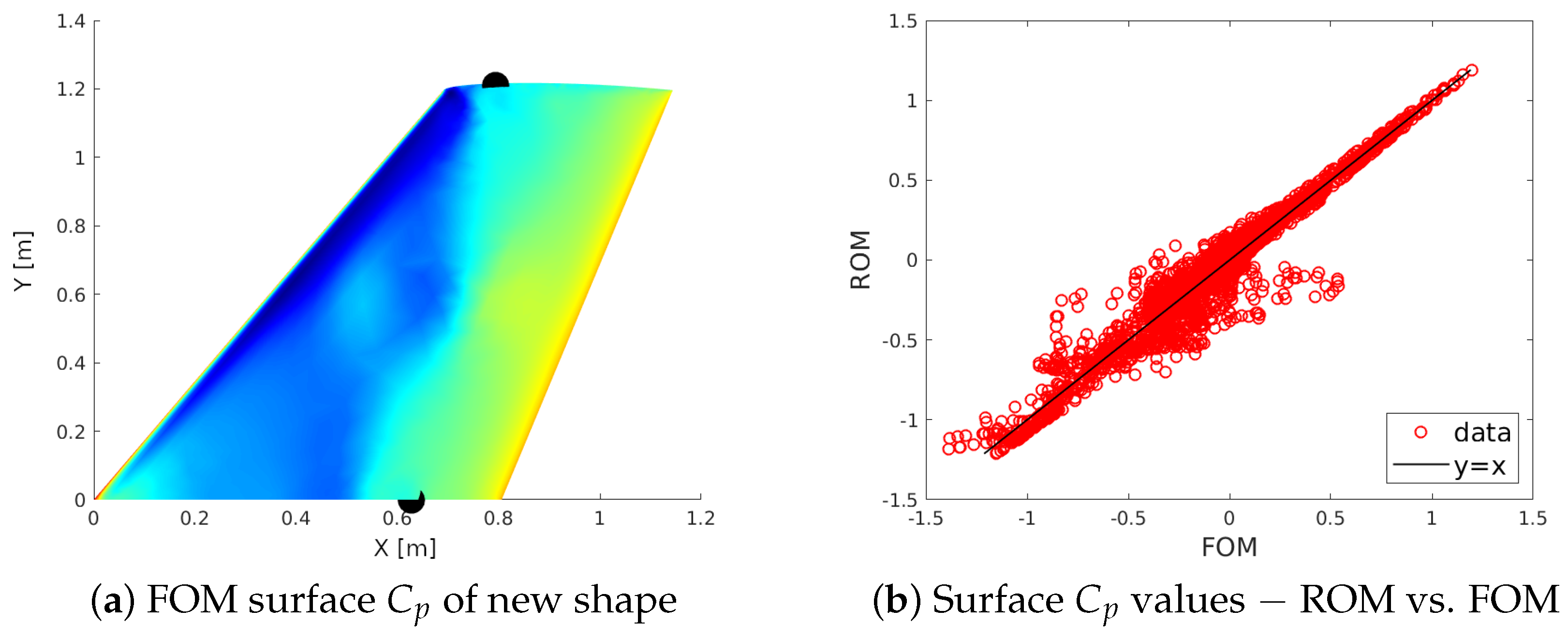
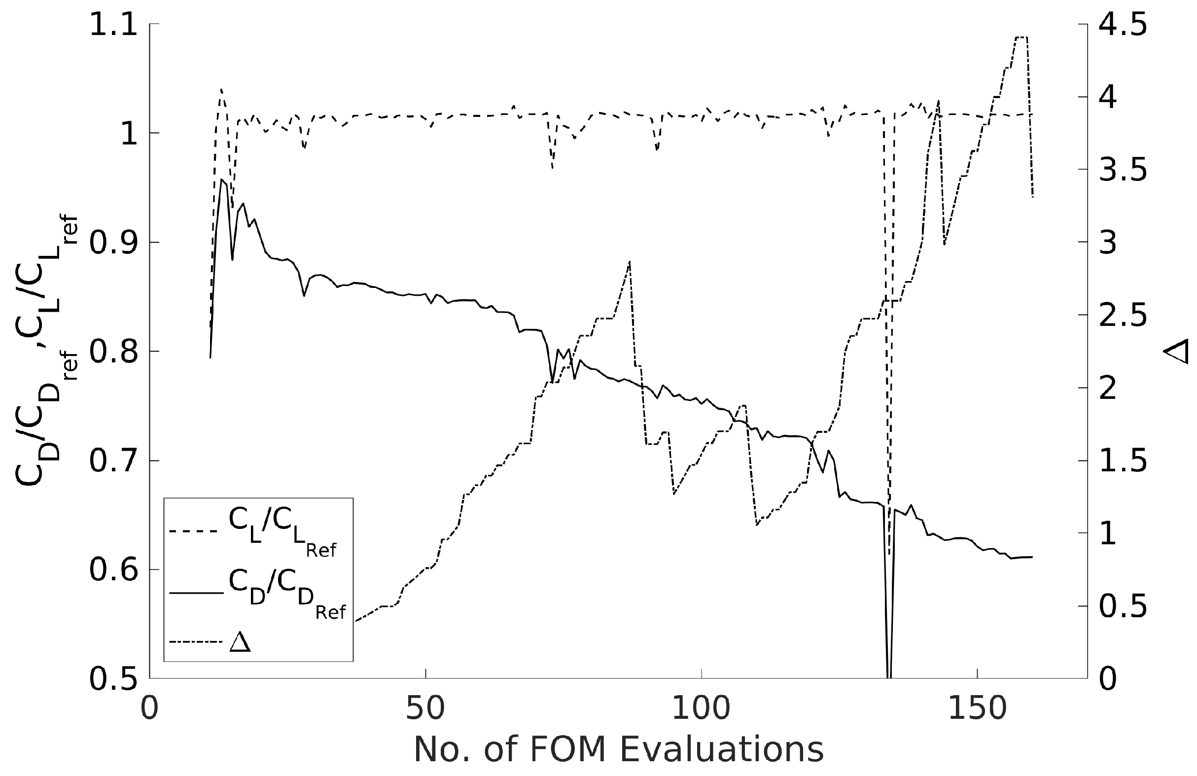
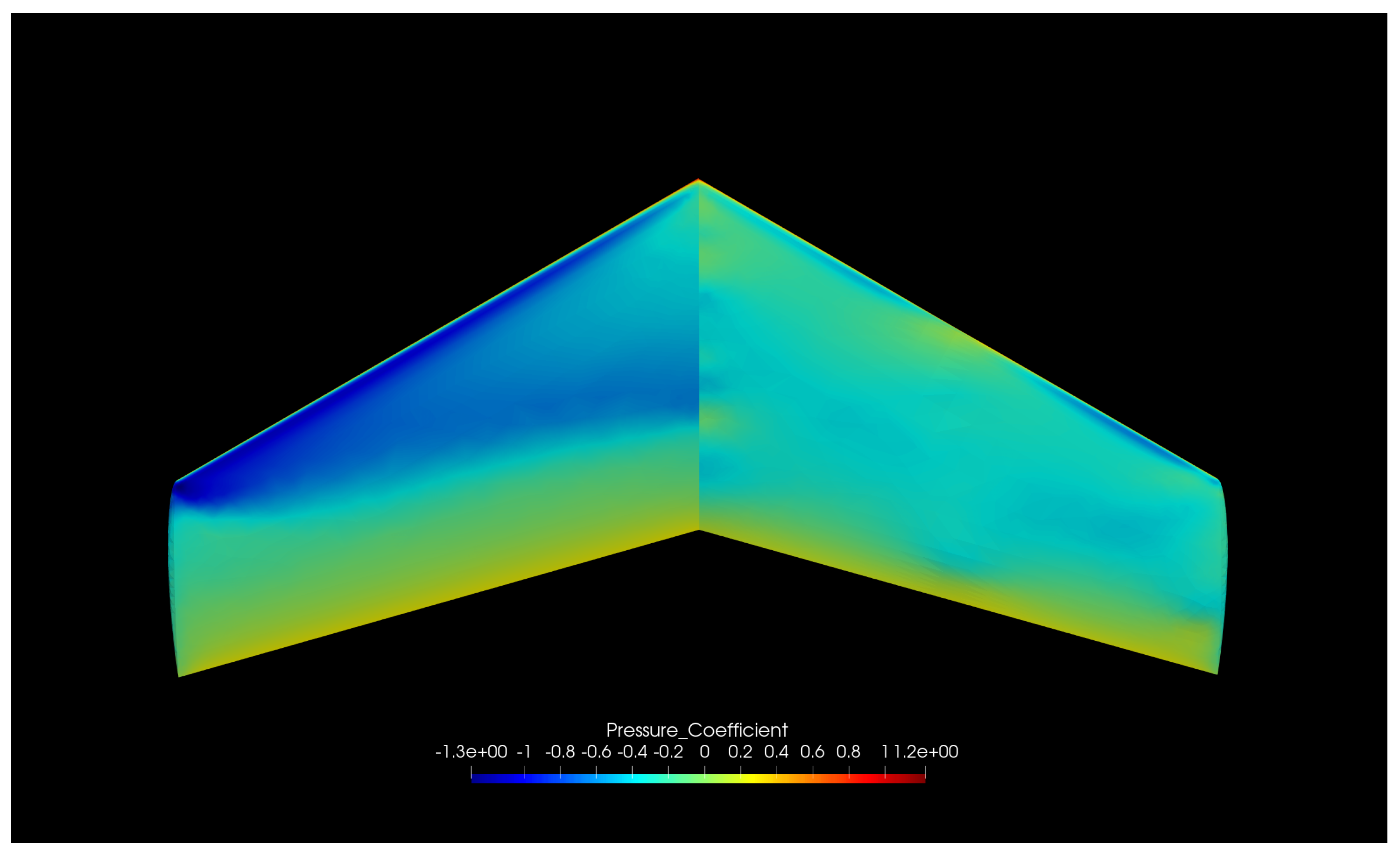
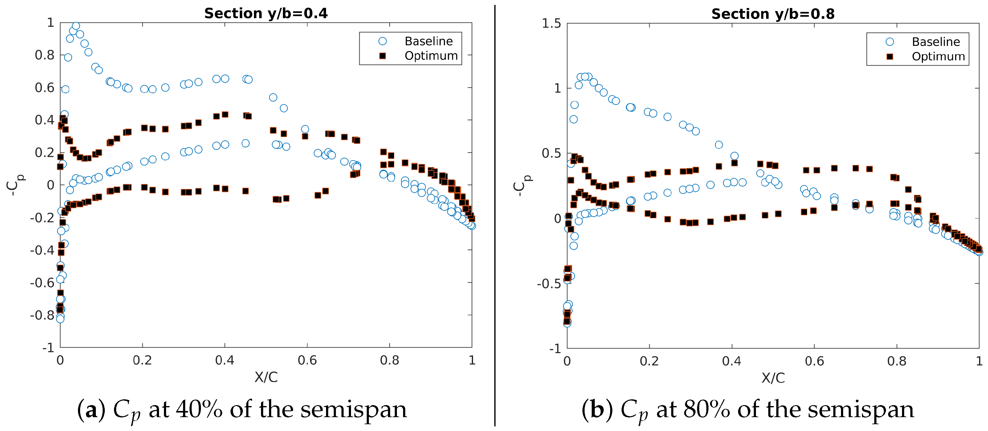
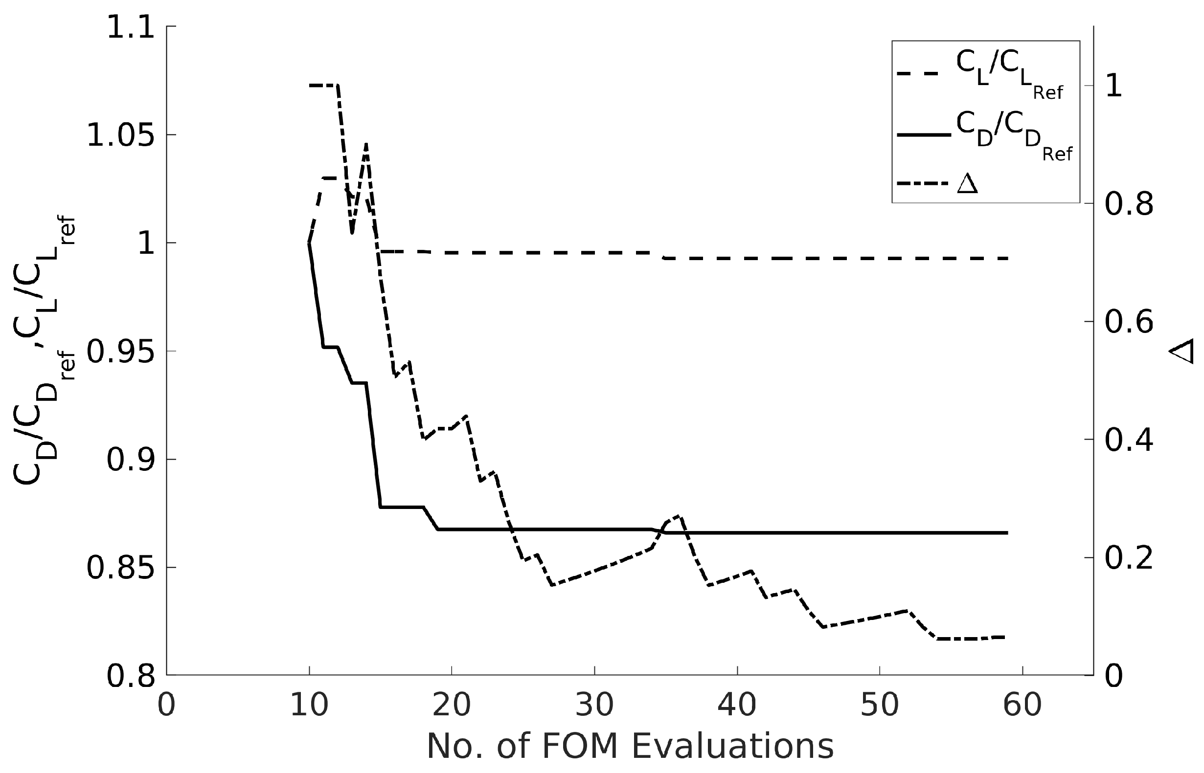
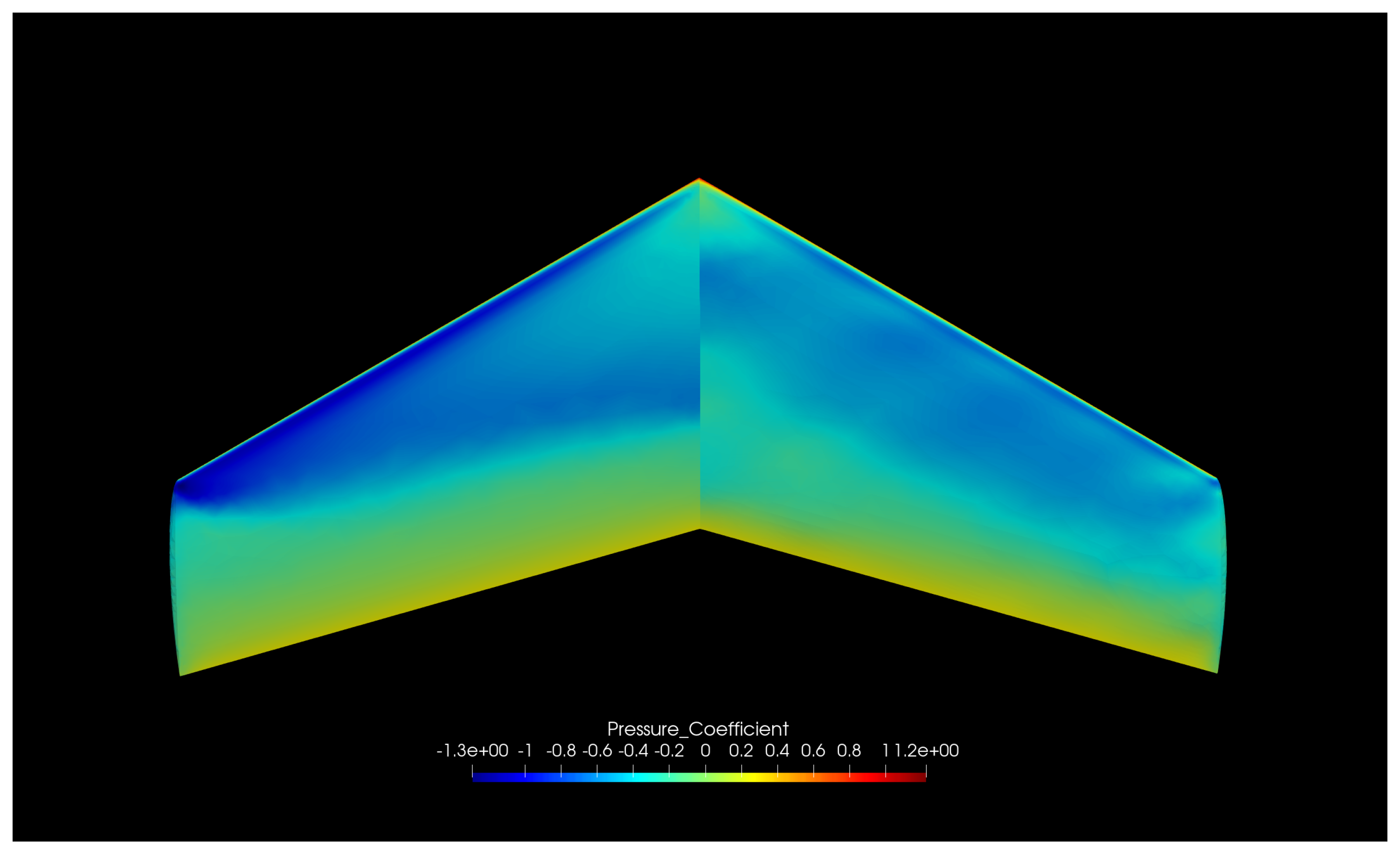
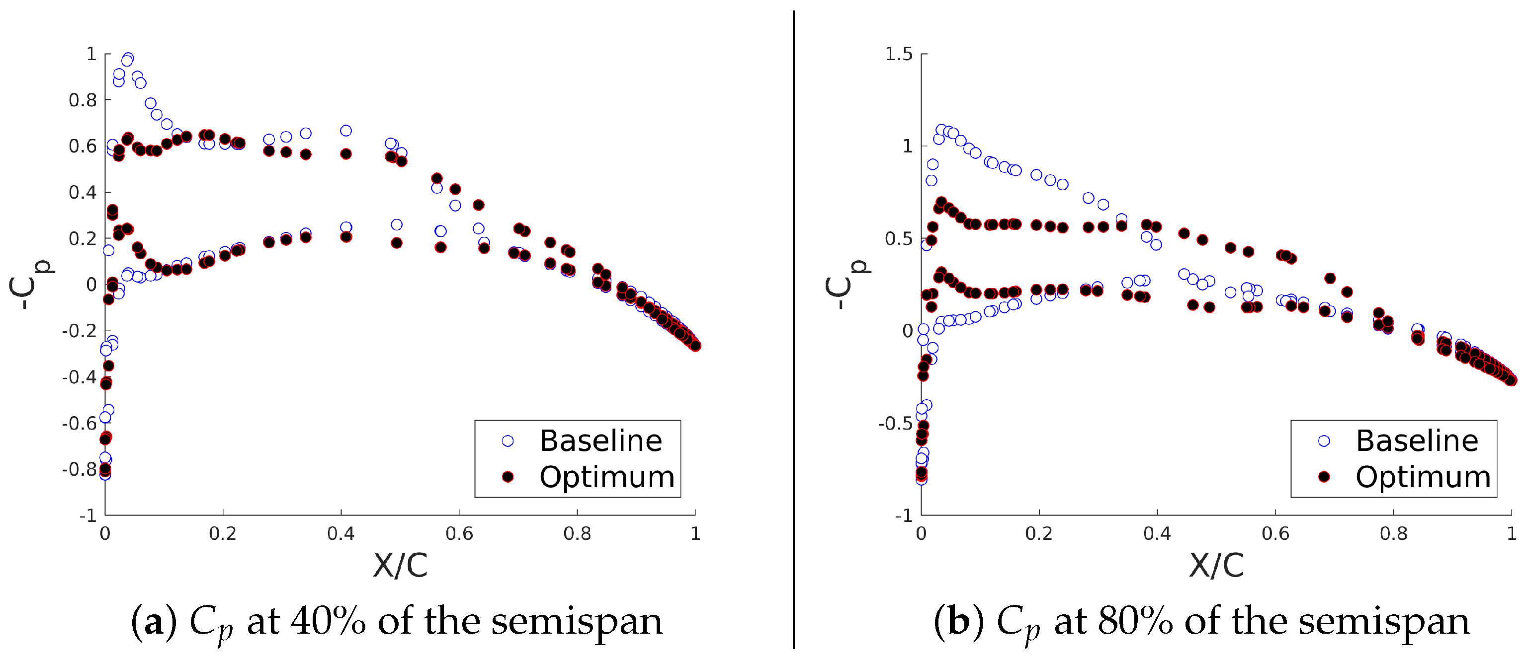
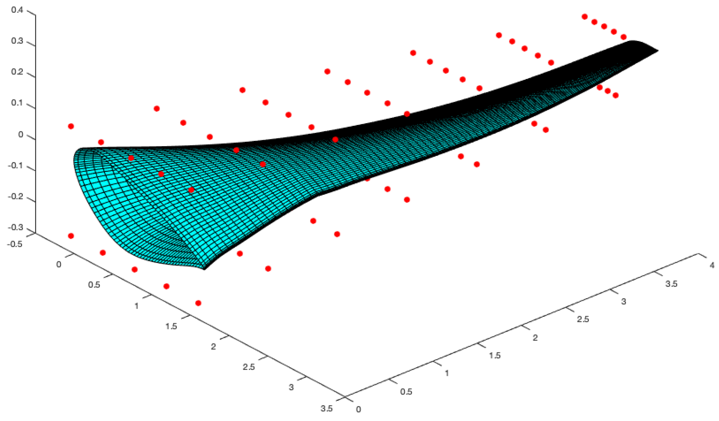
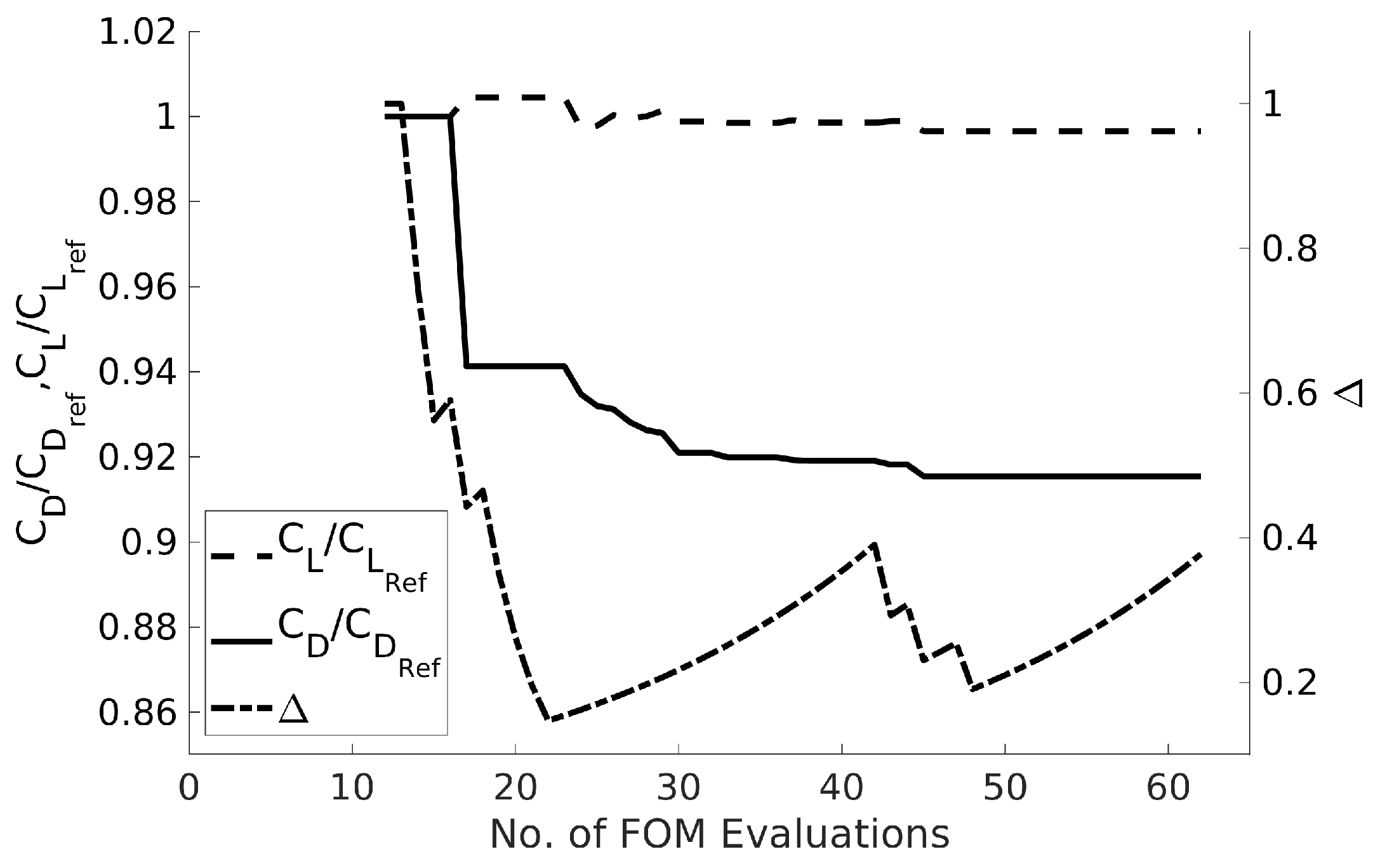
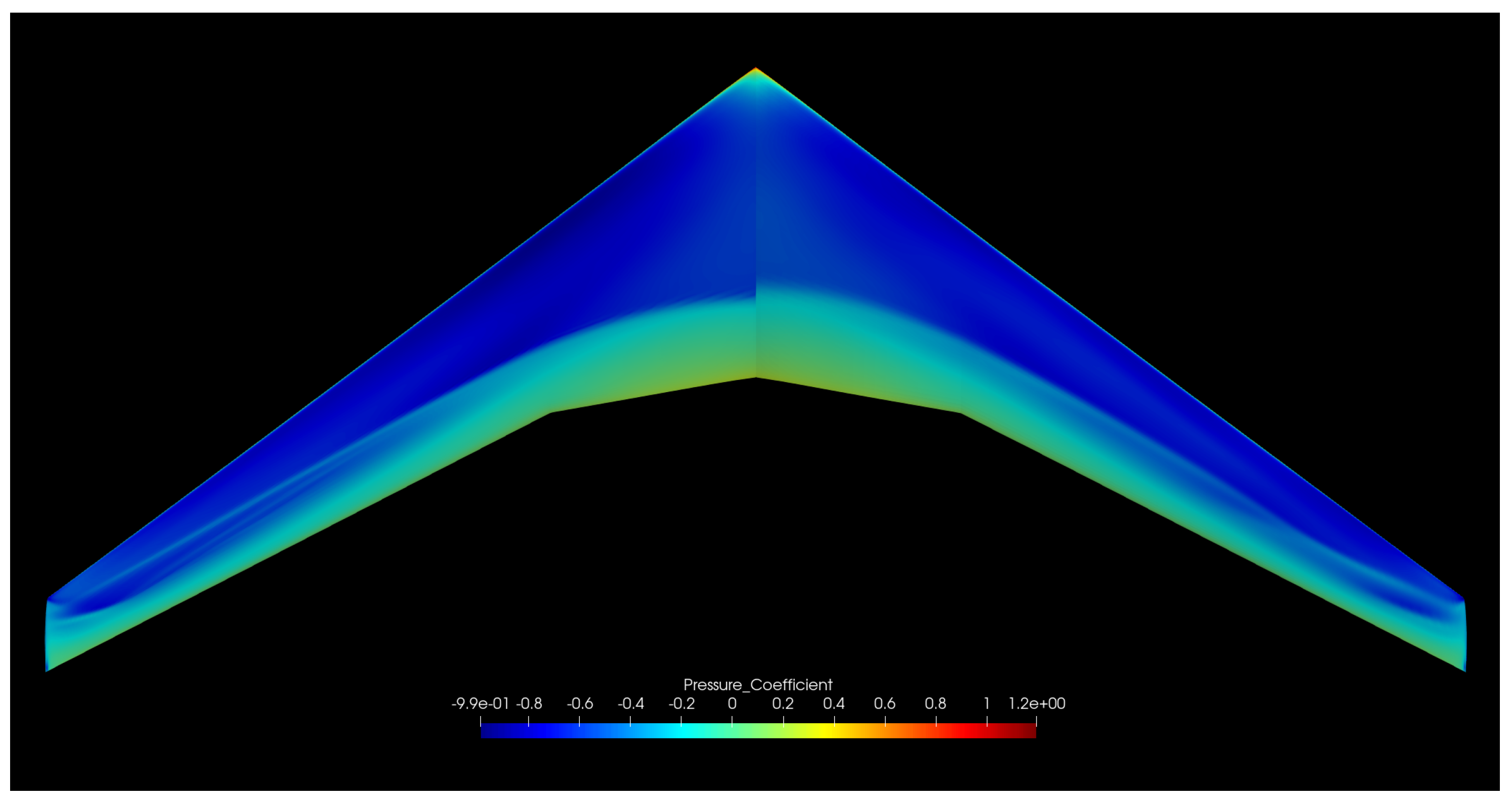
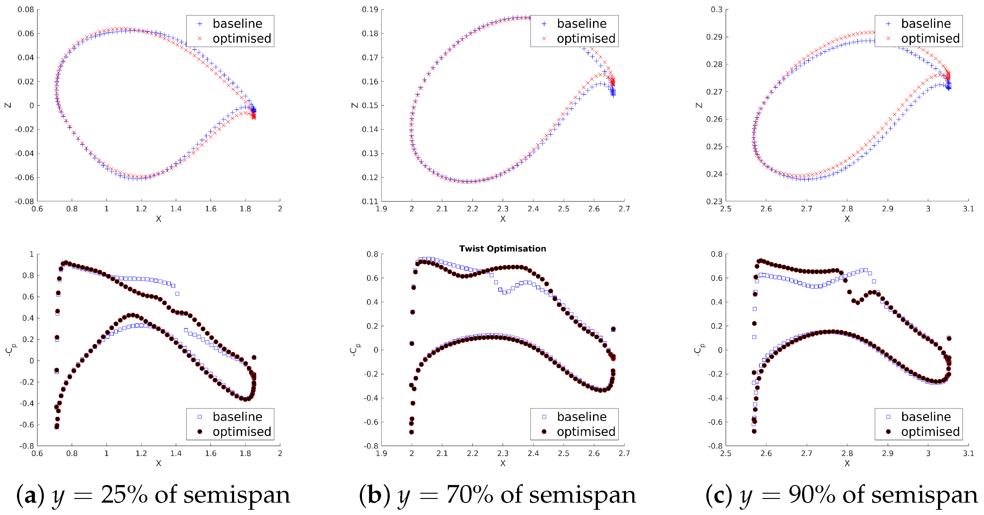
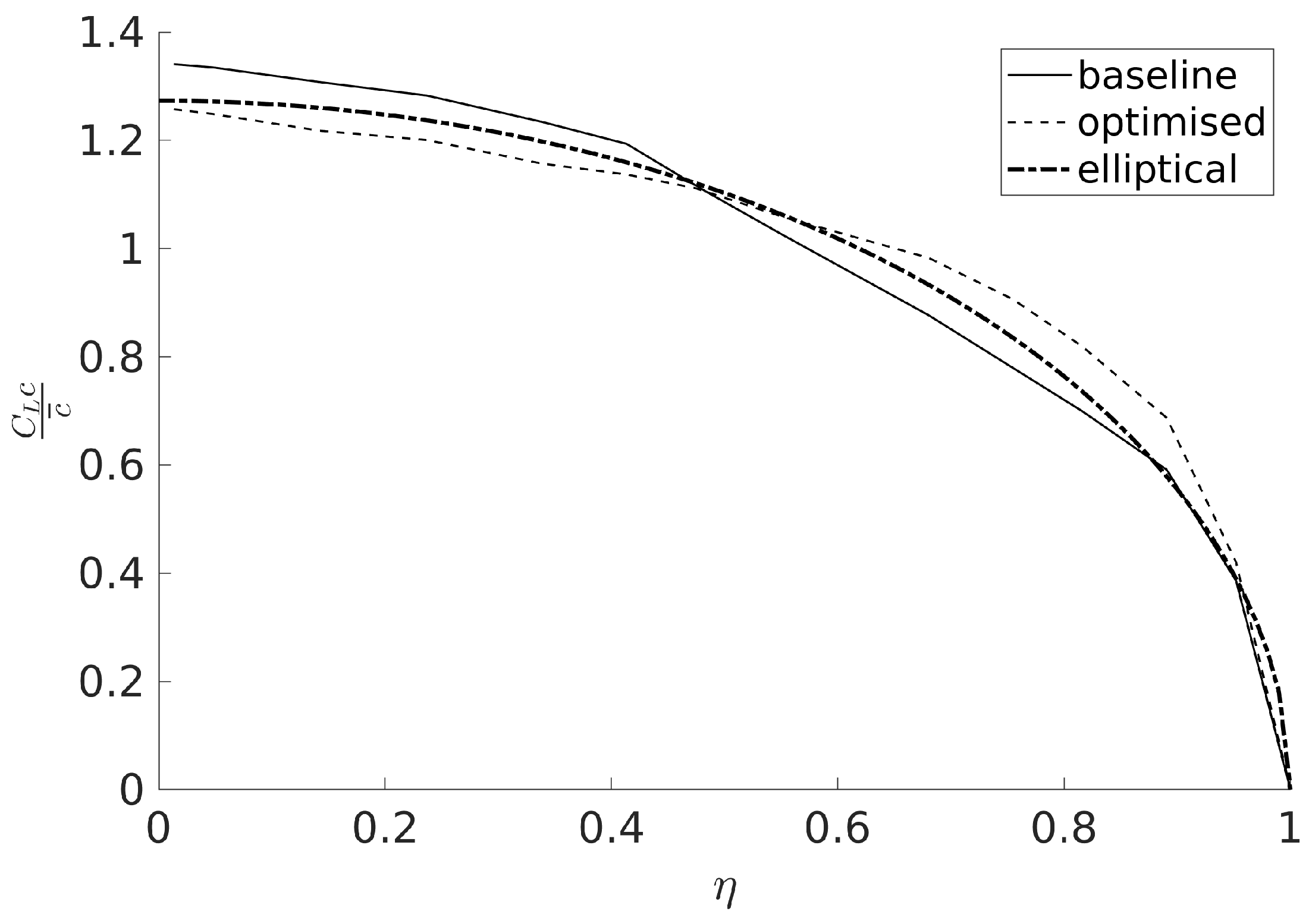
3.2. CRM Wing Test Case

Recall that for the DEIM to reconstruct the surface variables, it requires the solution at the DEIM points, which are interpolated based on their respective positions. Hence, the next test case assesses the methodology using a wing twist parameterisation. The test case is based on the AIAA Aerodynamic Design Optimization Discussion Group case 4.1 (data available online at: https://drive.google.com/file/d/107HHAUioOdiyFG_e63_S6R3TwlwsVM47/view, retrieved on 27 February 2023), which makes use of the wing geometry from the Common Research Model wing body configuration proposed for the AIAA Fifth Drag Prediction Workshop; full details of the model are given by Vassberg [37]. The result is a wing geometry representative of modern wide-body commercial airliner, with a span of approximately 59 m and a mean aerodynamic chord of 7 m. The flow problem set up corresponds to a flight condition with M = 0.85 at an angle of attack α = 2.2 ° , with a corresponding Reynolds number based on the mean aerodynamic chord of 5 × 10 6 . This test case is investigated in depth by Lyu et al. [41] using an adjoint solver; the authors provide and assess a series of meshes, which are also used in this study (meshes obtained from https://data.mendeley.com/datasets/7jnyjdbvf9/1, accessed on 10 June 2020). Table 1 shows a grid convergence study comparison between the SU2 results obtained as part of this work and those from Lyu et al., showing very good agreement. Lyu et al. show that the coarse mesh captures the design space trends adequately; hence, only that mesh is used in this optimisation study.
The selected mesh contains approximately 450 thousand elements, of which about 11 thousand are on the surface. The control points are organised in seven sets, equally spread along the span of the wing, resulting in seven design variables to control the local wing twist at each station. The normalised surface model, including the sections used as design variables is shown in Figure 12.
The optimisation problem definition is identical to the previous test case:
minimise μ D C D subject to C L > 0.50 ,
where μ represents the different wing twist angles at each span location and C L corresponds to the CRM design lift coefficient. The ROM was initialised with 10 random samples, generated using Latin hypercube sampling from a uniform distribution, with bounds [ 0.5 ° , 0.5 ° ] .
The optimisation convergence history is given in Figure 13; results show a decrease in drag of just over 8 % . Similarly to the last case, the trust region radius decreased rapidly, however, with new samples, the accuracy of the ROM increased, leading to further gains, and eventually, the improvements became less than a set threshold, and the optimiser stopped after 51 iterations.
An overview of the surface pressure coefficient is shown in Figure 14; results indicate a slight attenuation of the shock pattern on the upper surface, particularly in the inboard and wing tip regions. This is consistent with the the local effects of the optimisation shown in Figure 15.
Of course, wave drag is not the only contributor to the wing’s aerodynamic performance; Figure 16 shows a comparison between the span loadings of the original and optimised wings against an elliptical load distribution. Results indicate that the baseline wing should reduce the inboard lift and increase the lift produced outboard, which is what the optimised wing loading does. However, the new loading outboard exceeds the ideal case and the lift inboard mostly undershoots the elliptical loading, suggesting that any improvements to the induced drag are marginal at best. However, the overall effect is a drag reduction of about 8 % .

4. Conclusions

A new surrogate-based optimisation strategy is proposed using a POD-DEIM ROM to replace full-order CFD simulations. The ROM uses the POD-DEIM to reconstruct surface flowfields of the quantities of interest; the reconstructed variable values at the DEIM points required for the field reconstructions were interpolated and obtained using an RBF neural network based on the position of the DEIM points on the shapes proposed by the optimiser. The resultant framework is able to approximate flowfields for transonic, viscous problems with a relative small number of POD bases, i.e., requiring a limited number of snapshots. The optimisation framework was completed with a TRMM algorithm that manages the optimisation and triggers new samples that are used to enrich the ROM as the optimisation progresses. The framework was tested against two transonic wing cases. The results obtained demonstrate the ROM-based surrogate model to be a practical, nonintrusive method for problems with a moderate number of design variables, without compromising the critical physics of the problem or the performance of the optimiser.

Author Contributions

Conceptualization, S.M. and W.Y.; methodology, S.M. and L.K.; software, S.M., L.K. and W.Y.; validation, L.K.; formal analysis, S.M., W.Y. and L.K.; investigation, S.M., L.K. and T.T.R.; resources, S.M., L.K. and T.T.R.; data curation, S.M. and L.K.; writing—original draft preparation, S.M. and L.K.; writing—review and editing, S.M., W.Y. and T.T.R.; supervision, S.M. and T.T.R.; project administration, T.T.R.; funding acquisition, T.T.R. and S.M. All authors have read and agreed to the published version of the manuscript.

Funding

This research was funded by the U.K. Engineering and Physical Sciences Research Council Grant No. EP/P025692/1.

Institutional Review Board Statement

Not applicable.

Informed Consent Statement

Not applicable.

Data Availability Statement

Data available upon request from corresponding author.

Acknowledgments

The support from the University of Surrey High-Performance Computer Eureka is gratefully acknowledged.

Conflicts of Interest

The authors declare no conflict of interest.

Abbreviations

Latin Symbols
A Snapshot matrix
C D drag coefficient
C L lift coefficient
C p pressure coefficient
c DEIM coefficients
C E equality constraint
C I inequality constraint
Eenergy per unit mass
F objective function
l b design parameter lower bound values
M free-stream Mach number
Nnumber of points in full-order model
n p number of optimisation design variables
n r number of reduced bases
n s number of samples to build ROM
ppressure
DEIM interpolation indices matrix
R vector of fluid equation residuals
soptimisation step
S eigenvalues of snapshot matrix
T M reduced-basis matrix
T left singular vectors
u b design parameter upper bound values
V right singular vectors
w conserved flow variables
U velocity vector
u vector containing surface pressures
Greek Symbols
α step length for Newtown method, angle of attack
Δ trust region radius
δ 1 , δ 2 trust region effectiveness thresholds
η nondimensional span location
μ design parameters
ρ density
τ w wall shear stress
Mixed Symbols
ρ E energy per unit volume
ρ U momentum per unit volume

References

  1. Pironneau, O. Optimal Shape Design for Elliptic Systems; Springer Series in Computational Physics; Springer: Berlin/Heidelberg, Germany, 1984. [Google Scholar] [CrossRef]
  2. Jameson, A. Aerodynamic design via control theory. J. Sci. Comput. 1988, 3, 233–260. [Google Scholar] [CrossRef]
  3. Jameson, A.; Martinelli, L.; Pierce, N. Optimum aerodynamic design using the Navier–Stokes equations. Theor. Comput. Fluid Dyn. 1998, 10, 213–237. [Google Scholar] [CrossRef]
  4. Elliott, J.; Peraire, J. Practical three-dimensional aerodynamic design and optimization using unstructured meshes. AIAA J. 1997, 35, 1479–1485. [Google Scholar] [CrossRef]
  5. Nielsen, E.J.; Anderson, W.K. Aerodynamic design optimization on unstructured meshes using the Navier-Stokes equations. AIAA J. 1999, 37, 1411–1419. [Google Scholar] [CrossRef]
  6. Giles, M.B.; Pierce, N.A. An Introduction to the Adjoint Approach to Design. Flow Turbul. Combust. 2000, 65, 393–415. [Google Scholar] [CrossRef]
  7. Knill, D.L.; Giunta, A.A.; Baker, C.A.; Grossman, B.; Mason, W.H.; Haftka, R.T.; Watson, L.T. Response surface models combining linear and Euler aerodynamics for supersonic transport design. J. Aircr. 1999, 36, 75–86. [Google Scholar] [CrossRef]
  8. Kumano, T.; Jeong, S.; Obayashi, S.; Ito, Y.; Hatanaka, K.; Morino, H. Multidisciplinary design optimization of wing shape for a small jet aircraft using kriging model. In Proceedings of the 44th AIAA Aerospace Sciences Meeting and Exhibit, Reno, NV, USA, 9–12 January 2006; p. 932. [Google Scholar] [CrossRef]
  9. Hashimoto, A.; Jeong, S.; Obayashi, S. Aerodynamic optimization of near-future high-wing aircraft. Trans. Jpn. Soc. Aeronaut. Space Sci. 2015, 58, 73–82. [Google Scholar] [CrossRef]
  10. Toal, D.J.; Bressloff, N.; Keane, A.; Holden, C. The development of a hybridized particle swarm for kriging hyperparameter tuning. Eng. Optim. 2011, 43, 675–699. [Google Scholar] [CrossRef]
  11. Jahangirian, A.; Shahrokhi, A. Aerodynamic shape optimization using efficient evolutionary algorithms and unstructured CFD solver. Comput. Fluids 2011, 46, 270–276. [Google Scholar] [CrossRef]
  12. Schmitz, A. Constructive Neural Networks for Function Approximation and Their Application to CFD Shape Optimization. Ph.D. Thesis, Claremont Graduate University, California State University, Long Beach, CA, USA, 2007. [Google Scholar]
  13. Padron, A.S.; Alonso, J.J.; Eldred, M.S. Multi-fidelity methods in aerodynamic robust optimization. In Proceedings of the 18th AIAA Non-Deterministic Approaches Conference, San Diego, CA, USA, 4–8 January 2016; p. 0680. [Google Scholar] [CrossRef]
  14. Monschke, J.A.; Eldred, M.S. Multilevel-multifidelity acceleration of PDE-constrained optimization. In Proceedings of the 58th AIAA/ASCE/AHS/ASC Structures, Structural Dynamics, and Materials Conference, Grapevine, TX, USA, 9–13 January 2017; p. 0132. [Google Scholar] [CrossRef]
  15. Sirovich, L. Turbulence and the dynamics of coherent structures. I: Coherent Structures. II: Symmetries and Transformations. III: Dynamics and Scaling. Q. Appl. Math. 1987, 45, 583–590. [Google Scholar] [CrossRef]
  16. Willcox, K.; Peraire, J. Balanced model reduction via the proper orthogonal decomposition. AIAA J. 2002, 40, 2323–2330. [Google Scholar] [CrossRef]
  17. Rowley, C.W. Model Reduction for Fluids, using Balanced Proper Orthogonal Decomposition. Int. J. Bifurc. Chaos 2005, 15, 997–1013. [Google Scholar] [CrossRef]
  18. Ammar, A.; Mokdad, B.; Chinesta, F.; Keunings, R. A new family of solvers for some classes of multidimensional partial differential equations encountered in kinetic theory modeling of complex fluids. J. Non-Newton. Fluid Mech. 2006, 139, 153–176. [Google Scholar] [CrossRef]
  19. Lucia, D.J.; Beran, P.S.; Silva, W.A. Reduced-order modeling: New approaches for computational physics. Prog. Aerosp. Sci. 2004, 40, 51–117. [Google Scholar] [CrossRef]
  20. Noack, B.R.; Morzynski, M.; Tadmor, G. Reduced-Order Modelling for Flow Control; Springer Science & Business Media: Berlin/Heidelberg, Germany, 2011; Volume 528. [Google Scholar]
  21. Lassila, T.; Manzoni, A.; Quarteroni, A.; Rozza, G. Model order reduction in fluid dynamics: Challenges and perspectives. In Reduced Order Methods for Modeling and Computational Reduction; Springer: Berlin/Heidelberg, Germany, 2014; pp. 235–273. [Google Scholar] [CrossRef]
  22. Benner, P.; Gugercin, S.; Willcox, K. A Survey of Projection-Based Model Reduction Methods for Parametric Dynamical Systems. SIAM Rev. 2015, 57, 483–531. [Google Scholar] [CrossRef]
  23. Amsallem, D.; Farhat, C.; Haasdonk, B. Special Issue on Model Reduction. Int. J. Numer. Methods Eng. 2015, 102, 931–932. [Google Scholar] [CrossRef]
  24. Yondo, R.; Andrés, E.; Valero, E. A review on design of experiments and surrogate models in aircraft real-time and many-query aerodynamic analyses. Prog. Aerosp. Sci. 2018, 96, 23–61. [Google Scholar] [CrossRef]
  25. LeGresley, P.; Alonso, J. Airfoil design optimization using reduced order models based on proper orthogonal decomposition. In Proceedings of the Fluids 2000 Conference and Exhibit, Denver, CO, USA, 19–22 June 2000; p. 2545. [Google Scholar] [CrossRef]
  26. Demo, N.; Tezzele, M.; Mola, A.; Rozza, G. A complete data-driven framework for the efficient solution of parametric shape design and optimisation in naval engineering problems. arXiv 2019. [Google Scholar] [CrossRef]
  27. Manzoni, A.; Quarteroni, A.; Rozza, G. Shape optimization for viscous flows by reduced basis methods and free-form deformation. Int. J. Numer. Methods Fluids 2012, 70, 646–670. [Google Scholar] [CrossRef]
  28. Quarteroni, A.; Rozza, G. Optimal control and shape optimization of aorto-coronaric bypass anastomoses. Math. Model. Methods Appl. Sci. 2003, 13, 1801–1823. [Google Scholar] [CrossRef]
  29. Zahr, M.; Charbel, F. Progressive construction of a parametric reduced-order model for PDE-constrained optimization. Int. J. Numer. Methods Eng. 2015, 102, 1111–1135. [Google Scholar] [CrossRef]
  30. Carlberg, K.; Bou-Mosleh, C.; Farhat, C. Efficient non-linear model reduction via a least-squares Petrov-Galerkin projection and compressive tensor approximations. Int. J. Numer. Methods Eng. 2011, 86, 155–181. [Google Scholar] [CrossRef]
  31. Yao, W.; Marques, S.; Robinson, T.; Armstrong, C.; Sun, L. A reduced-order model for gradient-based aerodynamic shape optimisation. Aerosp. Sci. Technol. 2020, 106, 106120. [Google Scholar] [CrossRef]
  32. Yao, W.; Marques, S. Nonlinear aerodynamic and aeroelastic model reduction using a discrete empirical interpolation method. AIAA J. 2017, 55, 624–637. [Google Scholar] [CrossRef]
  33. Chaturantabut, S.; Sorensen, D.C. Nonlinear model reduction via discrete empirical interpolation. SIAM J. Sci. Comput. 2010, 32, 2737–2764. [Google Scholar] [CrossRef]
  34. Inc., T.M. MATLAB version: 9.13.0 (R2022b). 2022. Available online: https://www.mathworks.com/help/matlab/index.html?s_tid=CRUX_topnav (accessed on 5 March 2023).
  35. Schmitt, V.; Charpin, F. Pressure Distributions on the ONERA M6 Wing at Transonic Mach Numbers. Report of the Fluid Dynamics Panel Working Group 04. AGARD AR-138, May 1979. pp. B1–B44. Available online: https://tdl.libra.titech.ac.jp/journaldocs/recordID/article.bib-01/ZR000000447025?hit=-1&caller=xc-search (accessed on 5 March 2023).
  36. Mayeur, J.; Dumont, A.; Destarac, D.; Gleize, V. RANS simulations on TMR test cases and M6 wing with the Onera elsA flow solver. AIAA Pap. 2015, 1745, 2015. [Google Scholar] [CrossRef]
  37. Vassberg, J.; Dehaan, M.; Rivers, M.; Wahls, R. Development of a common research model for applied CFD validation studies. In Proceedings of the 26th AIAA Applied Aerodynamics Conference, Honolulu, HI, USA, 18–21 August 2008; p. 6919. [Google Scholar] [CrossRef]
  38. Economon, T.D.; Palacios, F.; Copeland, S.R.; Lukaczyk, T.W.; Alonso, J.J. SU2: An Open-Source Suite for Multiphysics Simulation and Design. AIAA J. 2016, 54, 828–846. [Google Scholar] [CrossRef]
  39. Lapuh, R. Mesh Morphing Technique used with Open-Source CFD Toolbox in Multidisciplinary Design Optimisation. 2018. Available online: https://www.semanticscholar.org/paper/Mesh-Morphing-Technique-used-with-Open-Source-CFD-Lapuh/f18ed2bea4fead68a08d248d16b9b6b17d5123af (accessed on 5 March 2023).
  40. Agarwal, D. Shape optimization using feature-based CAD systems and adjoint methods. Ph.D. Thesis, Queen’s University Belfast, Belfast, UK, 2018. [Google Scholar]
  41. Lyu, Z.; Kenway, G.K.; Martins, J.R. Aerodynamic shape optimization investigations of the common research model wing benchmark. AIAA J. 2015, 53, 968–985. [Google Scholar] [CrossRef]
Figure 1. ROM shape optimisation flow chart.
Aerospace 10 00470 g001
Figure 2. Onera M6 grid convergence.
Aerospace 10 00470 g002
Figure 3. Onera M6 baseline mesh: (a) surface and symmetry plane; (b) surface mesh and associated control points.
Aerospace 10 00470 g003
Figure 4. Assessment of ROM reconstruction at two sample points.
Aerospace 10 00470 g004
Figure 5. Assessment of ROM prediction at new sample point.
Aerospace 10 00470 g005
Figure 6. Onera M6 lift constrained optimisation convergence.
Aerospace 10 00470 g006
Figure 7. Upper surface pressure comparison. Left side: baseline; right side: optimum.
Aerospace 10 00470 g007
Figure 8. Onera M6 pressure coefficient.
Aerospace 10 00470 g008
Figure 9. Onera M6 lift and thickness constrained optimisation convergence.
Aerospace 10 00470 g009
Figure 10. Upper surface pressure comparison. Left side: baseline; right side: optimised.
Aerospace 10 00470 g010
Figure 11. Onera M6 pressure coefficient.
Aerospace 10 00470 g011
Figure 12. CRM wing baseline shape.
Aerospace 10 00470 g012
Figure 13. Comparison of optimisations with random initial ROM data.
Aerospace 10 00470 g013
Figure 14. Upper surface pressure coefficient. Left side: baseline; right side: optimised.
Aerospace 10 00470 g014
Figure 15. CRM wing section modifications and corresponding surface pressure coefficient at different span locations.
Aerospace 10 00470 g015
Figure 16. Comparison of different span loadings.
Aerospace 10 00470 g016
Table 1. SU2 grid convergence study and comparison with respect to reference [41].
Mesh LevelMesh Size C D —[41] C D —SU2
L028,835,8400.019970.02007
L13,604,4800.020170.02034
L2450,5600.021110.02169
Disclaimer/Publisher’s Note: The statements, opinions and data contained in all publications are solely those of the individual author(s) and contributor(s) and not of MDPI and/or the editor(s). MDPI and/or the editor(s) disclaim responsibility for any injury to people or property resulting from any ideas, methods, instructions or products referred to in the content.

