On the Possibility of Cross-Flow Vortex Cancellation by Plasma Actuators

Abstract

Cancellation of the cross-flow vortices in a swept-wing boundary layer is attempted by plasma actuator array in numerical simulation. The response of the boundary layer to the stationary excitation by a single actuator section is measured experimentally and compared to the response obtained from the solution to the parabolized stability equations. A linear approach is shown to be held within the peak-to-peak magnitude of the stationary cross-flow vortices below 10% of the local potential flow velocity. Within the linear model, an optimal control strategy and a faster suboptimal one are developed to calculate voltage amplitude distribution across the electrodes, taking into account the forcing constraints. Simulation of the cancellation process is performed, showing up to a 20 dB reduction in the initial spanwise velocity modulation in the boundary layer. The minimal actuator resolution required for the successive implementation of the control is shown to be in the order of a quarter of the most amplified wavelength, or 3–4 displacement thickness of the boundary layer. Linear estimates predict up to a 150 mm (22% of flow acceleration region length) transition delay for an actuator momentum coefficient of 0.005%.

1. Introduction

Turbulent drag is one of the major contributors to airplane total drag at cruise conditions, and thus, extensive research efforts are made to postpone the transition to turbulence on the airplane wing. The wings of most modern airplanes are tapered, which means that a three-dimensional boundary layer is formed near the streamlined surface. Swept (that is, with constant chord) wing configuration is frequently used to simplify the problem and yet model the behavior of the boundary layer flow.

For the swept configuration, two types of instabilities are present in the boundary layer: Tollmien–Schlichting (TS) waves and cross-flow (CF) instabilities [1,2,3,4,5]. TS waves become marginal at certain negative pressure gradients, and the transition to turbulence is governed by CF modes. CF modes can be understood as counter-rotating vortices, with their axes slightly inclined to the external streamline. Momentum transfer in these vortices leads to velocity modulation in the boundary layer, with the typical wavelength ~15–20 δ₁. The instability range for the CF mode spans over zero frequency; therefore, both travelling waves and stationary vortices are amplified in the boundary layer. Travelling waves are induced by external turbulence, while the stationary vortices are excited by roughness of the streamlined surface. In flight conditions, stationary disturbances dominate.

One of the control methods that has been demonstrated in lab studies for the transition delay is primary disturbance cancellation, which was first demonstrated for TS waves in [6,7]. Along with the artificial disturbance cancellation, which was demonstrated in these works, further research has shown the possibility of natural TS wave control [8,9]. For stationary CF modes, vortex cancellation for the artificial periodic surface roughness was recently shown in [10].

Plasma actuators have been studied as a flow control device over the last two decades. Generally, they can be defined as actuators that use electric, magnetic forces or heat release, which is created in the gas discharge plasma. A detailed review of plasma actuator types, physics and applications can be found in [11,12,13]. Gas discharges have historically been used as a source for the artificial hydrodynamic disturbances in the flow control or aeroacoustics problems. A more detailed review on this topic can be found in [14]. Most studies are related to dielectric barrier discharge plasma actuators, which utilize the ionic wind as a key mechanism of flow forcing.

Plasma actuators were studied as an instrument for the control of swept-wing boundary-layer instabilities. Transition delay was demonstrated due to cross-flow component profile modification by volume force [15,16]. The estimates [17,18] show that this technique can be energy-efficient even in cruise conditions, in contrast to the 2D boundary-layer case [19].

It was demonstrated [20] that spanwise-modulated discharge can be used to excite CF modes. Transition delay via a subcritical mode excitation by using PA has been attempted by several groups [20,21,22]; however, no positive results were obtained due to a relatively high unsteadiness of the barrier discharge, caused by wandering of micro-discharges [23,24]. In contrast, transition delay was demonstrated at a higher freestream turbulence level, in which travelling CF modes dominate in the boundary layer [25].

CF vortex cancellation by plasma actuators was attempted only theoretically and only for spanwise-periodic disturbance sources. It was shown that at least with some actuator configuration [26], vortex array with a constant magnitude can be damped by a periodic actuator array.

In this work, we tried to demonstrate the fundamental possibility of natural stationary CFI vortex cancellation by plasma actuators. It is assumed that a multichannel system can be built by sectioning the buried electrode in a manner of “plasma panel” [27], allowing control of the spanwise force distribution. An advantage of such a control strategy is reduced energy consumption compared with the modification of a cross-flow velocity profile in the boundary layer. Estimates based on force term scaling in Navier–Stokes equations reveal that both control methods require comparable volume force density $f^{\prime }~\rho u_e^2/R$. However, this force should be applied in the entire volume of the boundary layer (or in a substantial part of it) for cross-flow velocity reduction [28]. Cancellation of steady CF vortices requires a similar force density distributed in the short stripe of the boundary layer that is shorter than that of the steady mode period. The main goal of this paper is estimation of the possibility and effectiveness of such control and the actuator resolution required to make it possible.

The paper is structured as follows. In the first section, we describe the response of the boundary layer to the forcing by a single elementary plasma actuator. The disturbance structure that was obtained in numerical modeling and experimentation is compared. In the second section, an approach is proposed for the optimal control design for a line of elementary plasma actuators. Finally, CFI vortex cancellation is demonstrated in a numerical experiment based on both the calculated and measured boundary-layer response, and the results of a parametric study are presented.

2. Experimental and Numerical Approach

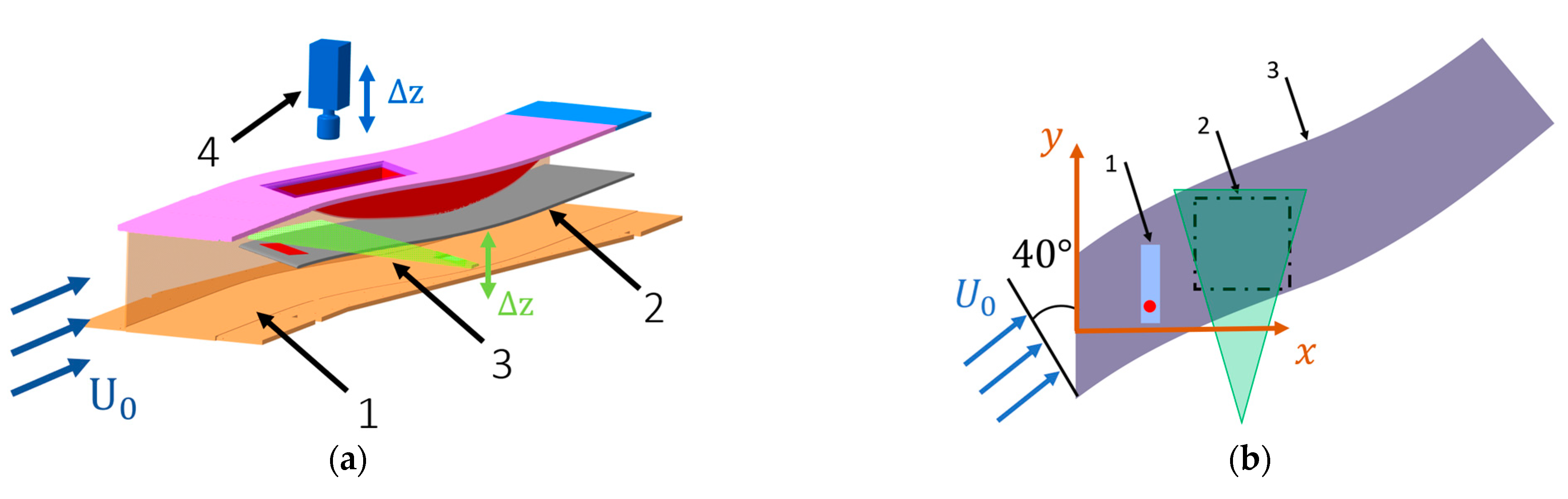
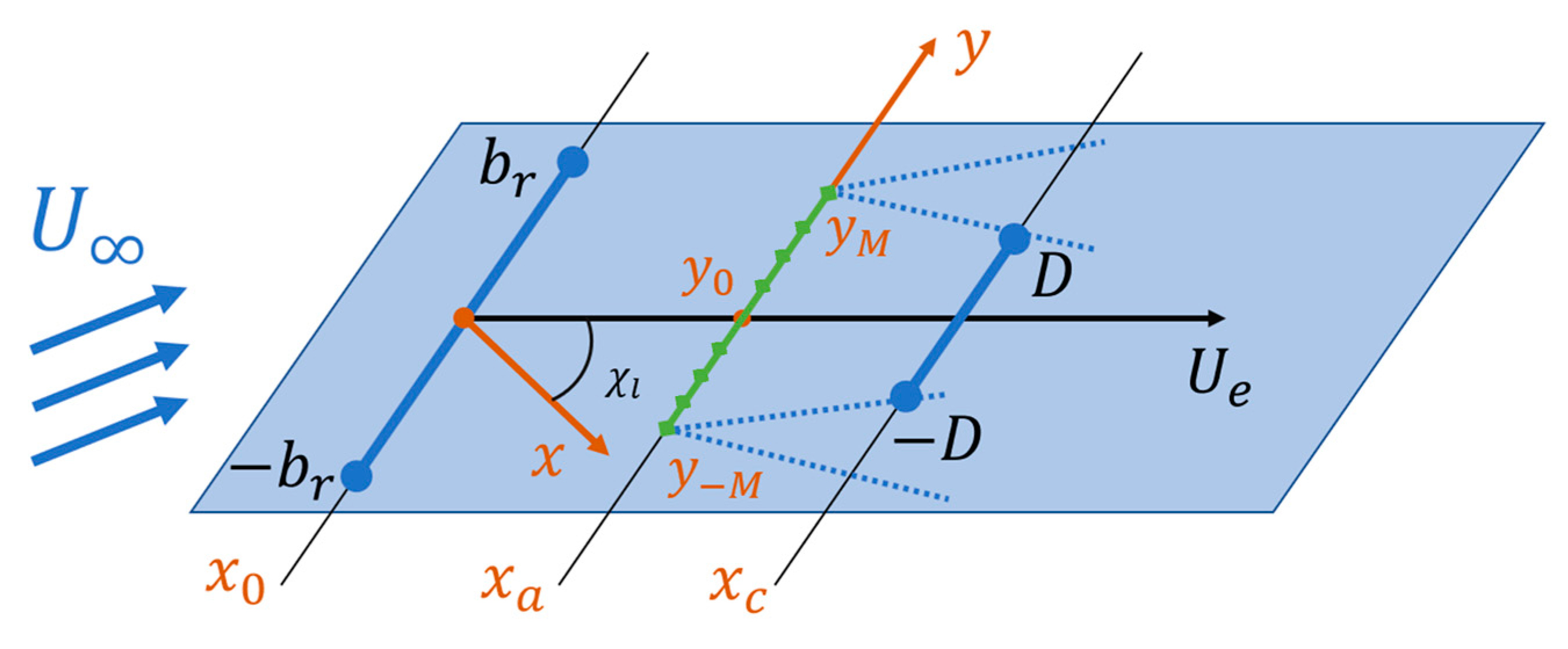
2.1. Experiment Design

The experiment was performed in an open-circuit subsonic wind tunnel D-3 in JIHT RAS. The settling chamber was equipped with a honeycomb, grids and nozzle with contraction 9:1. The wind tunnel had a cross-section 300 × 300 mm, and the maximal attained flow velocity was 50 m/s. With all grids installed, the turbulence level at the position 200 mm upstream of the model leading edge was less than 0.05%. Modeling of the accelerated boundary-layer conditions was carried out on a 12 mm flat plate manufactured from polished acrylic glass. The plate sweep angle was 40 degrees, and its leading was shaped to an 8:1 semi-ellipse. The plate was equipped with a trailing edge flap, which was installed at 3.5 degrees. The upper wall of the test section was shaped to provide an accelerating flow in the region X = 200–600 mm. The side walls were designed to follow the streamline outside the boundary layer.

A plasma actuator (Figure 1b) was constructed in an asymmetric configuration consisting of aluminum corona and copper underlying electrodes that were separated by a 1 mm thick ceramic dielectric (ε = 10.4). To localize the forcing region, the underlying electrode was shaped as a strip with a width of 2 mm. Sinuous voltage in the range of 3.0–5.0 kV was applied to the electrodes from a resonant power source at frequencies 100–110 kHz. The plasma actuator was mounted parallel to the leading edge at X = 200 mm, downstream of the neutral point for CFI modes. Prior to the measurements, the actuator was operated for 30 min to stabilize the oxide layer on the electrode [29]. This leads to a more homogeneous discharge structure and excludes the drift of the actuator characteristics during the run.

The characteristics of a plasma actuator with a limited active span of the electrode were studied in [30] by using a concept of a localized group of micro-discharges. It was shown that in a quiescent condition, the plasma actuator creates a three-dimensional wall jet with a pair of counter-rotating vortices at it sides. Quiescent flow can be modeled with two force components: one normal to electrode edge f_x, and the other one parallel to the edge and directed away from the micro-discharge group, f_y. For 190 kHz and 3.2 kV, thrust of the single actuator section was found to be 5 μN, f_y ~ 0.3–0.5 f_x. Assuming that thrust scales linearly with frequency, we obtain for the present condition the typical value of 2.9 μN per section. Heat release, which was again rescaled with frequency, can be estimated as 0.17 W per section.

Flow diagnostics was performed by using 2D PIV in a panoramic configuration (Figure 1a). The flow was illuminated by a two-pulse Nd:YAG laser with a pulse energy of 100 mJ and a wavelength of 532 nm, focused into a 0.3 mm thick laser sheet. Images were taken by a 16-bit CCD camera with a resolution of 2560 × 2160 pixels. The measurement plane was located parallel to the plate and moved with a spatial step of 0.1 mm along the wall-normal co-ordinate. At a frequency of 15 Hz, the statistics of 100 instantaneous pairs of images were measured. Images were processed with a cross-correlation algorithm with 16 × 16- to 6 × 6-pixel interrogation window size, which provided an in-plane spatial resolution of 0.36 mm.

Freestream velocity distribution, boundary-layer profiles and parameters are shown in Figure 2. Flow velocity scales with chordwise co-ordinate as U~(x₋x₀) for X < 550 mm. Spanwise velocity component was found to satisfy sweep condition V ≈ const with the accuracy of 5%. Boundary-layer profiles were measured in detail at flow velocity 7 m/s, then the results were scaled to test velocity by using R^1/2 scaling. Boundary-layer displacement thickness for 25 m/s is about δ₁ = 0.4 mm; its evolution corresponds well to the boundary-layer calculation. Cross-flow velocity has a typical jet-like profile, with a maximum attained at z = δ₁. The maximum of the cross-flow velocity is in the order of 7% U_e up to X = 450 mm, then drops due to straitening of the external streamline. In Figure 2, points correspond to experimental data, and lines correspond to the potential flow and boundary-layer calculation. One can see that in general, a reasonable likelihood is obtained between the designed and measured mean boundary-layer flow for X < 450 mm, rendering the setup that was used adequate for modelling of the swept-wing boundary-layer flow. Figure 2e shows the growth of the stationary disturbances in the boundary layer, which was obtained for the most growing wavelength of 6.8 mm.

2.2. Approach to the Cross-Flow Vortex Cancellation

The scheme of the control system for vortex cancellation is shown in Figure 3. Plasma actuator, which is parallel to the leading edge, has q elementary discharge sections and is located at the position x_a. Amplitudes of body forces induced by the actuator sections that are necessary for cross-flow vortex cancellation should be found from the measurements of boundary-layer perturbations in the row of similar amount control points located behind the actuator at distance x_c from the leading edge. In order to estimate the natural perturbations and the response of the boundary layer to each actuator section, the measurements should be performed in the cases of no actuation and for the unit forcing of each section. For the sake of simplicity, actuators sections and control points are assumed to be distributed uniformly along the span within the width 2b (see Figure 3). It is also assumed that perturbations in control points are characterized by a single relevant quantity, for example, by perturbation of the parallel-to-external streamline velocity component at distance z = 1.3 δ₁. For adequate system operation control, points should be shifted along the span with respect to the actuator taking into account the disturbances trajectory. The required shift was obtained from the results of computations of disturbances induced by a single actuator’s section. For a rather small distance, the disturbance maximum propagates approximately along the straight lines, with local sweep angle ${\chi }_l\cong {26.7}^0$. In subsequent theoretical consideration, this shift is taken into account by means of the introduction of shifted spanwise co-ordinate $y_s=y+\left(x-x_a\right)\cdot tg\left({\chi }_l\right)$. In shifted co-ordinates, the actuator and control points are located at the same points $y_{sn}=-m\cdot h ; m=-M\dots M$.

Within a certain amplitude of natural disturbances, the boundary layer is interpreted as a linear dynamic system, with q inputs (sections of plasma actuator). Define the system output as a vector of p velocity samples, which are calculated or taken by PIV at the position x_c and z ~ 1.3 δ₁. We do not specify internal system states; we simply assume that dimensions for the state vector, input and output are n, q = 2 M + 1 and p. In this case, the system can be written as follows:

$$\left\{\begin{array}{c}\dot{x}=Ax+Bu+Nw,\\ y=Cx,\end{array}\right.$$

(1)

where $x\in {ℝ}^{n\times 1}$—state vector, $u\in {ℝ}^{q\times 1}$—actuation amplitudes, $y\in {ℝ}^{p\times 1}$—output velocity vector, and $w\in {ℝ}^{r\times 1}$—external disturbance. $A\in {ℝ}^{n\times n}$, $B\in {ℝ}^{n\times q}$, $C\in {ℝ}^{p\times n}$—matrices with appropriate dimensions. We consider only time-invariant disturbances, that is, $w=\mathrm{const}$.

In asymptotically large time, we obtain $\dot{x}=0$, and (1) can be rewritten as

$$\left\{\begin{array}{c}0=Ax+Bu+Nw,\\ y=Cx.\end{array}\right.$$

(2)

At zero input ($u_{01}=0$), system output $y_{01}$ is determined as

$$y_{01}=-C{A}^{-1}N{w}_1.$$

(3)

Since the natural disturbances are always present in the system, system identification for stationary disturbances can be performed as follows. We excite the system by forcing individual actuator sections by unity signal as $u={\left. [0\dots ,1,\dots 0\right]}^T$. Then, the output vector is a superposition of system responses to natural and artificial excitation and

$$y_1-y_{01}=-C{A}^{-1}B{u}_1=P{u}_1.$$

(4)

Scanning the inputs, we obtain the equation for the determination of matrix P:

$$P=\left(Y-Y_0\right)I_q=\left(Y-Y_0\right),$$

(5)

where $Y=\left\{y_{11\dots }{y}_{1q}\right\}, Y_0=\left\{y_{01\dots }{y}_{0q}\right\}$—stacked system responses at consequent channel excitation, $I_q$—unity matrix.

Now we assume that the system is forced by external perturbation $w_2$, causing the output

$$y_{02}=-C{A}^{-1}N{w}_2,$$

(6)

We search for the vector $u_2$, minimizing the output $y_2$. The forced output is now written as

$$\begin{gathered} y_2=-C{A}^{-1}N{w}_2-C{A}^{-1}B{u}_2=y_{02}-Pu=0, \\ Pu=y_{02}. \end{gathered}$$

(7)

For the considered case, when the velocity is sampled at high resolution and the number of actuators is limited ($q<p$), the system (7) is solved by minimization of the cost function $\mathrm{J}=\Vert P{u}_2-y_{02}\Vert {}_2^2$, and the optimal solution is obtained as

$${\mathrm{u}}_2={\left(P^{T}P \right)}^{-1}{P}^T{y}_{02}.$$

(8)

Since the control of the disturbances is possible only across the central part of the actuator panel, we window the output vector with flat-top function by multiplying it by diagonal matrix $Q$. Additionally, we add the control penalty to the cost function $J=\Vert P{u}_2-y_{02}\Vert {}_2^2+\epsilon \Vert u_2\Vert {}_2^2$ that gives the optimal control solution as

$${\mathrm{u}}_2={\left(P^{T}P+\epsilon I\right)}^{-1}{P}^{T}Q{y}_{02}.$$

(9)

The construction of the plasma actuator limits the control to the positive values. To account for this, the following procedure is performed. The optimal solution $u_2$ is calculated in accordance with Equation (9). Then, the control values are shifted by a minimal value of $u_2$. This leads to the strictly positive amplitude vector $\widetilde{u_2}=u_2+min\left(u_2\right)$. Although this control is suboptimal for $u>0$, it does not affect the central part of the control region for high-enough actuator resolution.

An alternative approach is to perform the quadratic minimization task for J with the constraint $u>0$. The problem was solved via MATLAB routine based on the interior-point method.

Although the latter approach finds an optimal solution in the positive control value domain, the former one is much faster and can be used in real-time applications. The typical time for the solution of regression problem (7) on the Intel Core i9 PC is 0.03–0.07 ms; for that of the nonlinear optimization task, it is 1 ms.

Despite the rather simple control strategy developed here, the efficiency of its application in an experiment strongly depends on the spectrum of “natural” disturbances, pitch of the actuator sections and control points and other factors. The modeling of such control by using numerical and experimental models of natural disturbances and boundary-layer response to actuator forcing is described in the next sections of this paper.

2.3. Numerical Modeling of Cross-Flow Vortex Cancellation by DBD

2.3.1. Numerical Method

Theoretical analysis of both natural and discharge-induced disturbance development is based on the solution of parabolized stability equations (PSE). Non-dimensional variables are introduced by using oncoming flow velocity $u_{\infty }$ and characteristic boundary-layer thickness $\delta ={\left(\nu L/u_{\infty }\right)}^{1/2}$. Values of flow velocity $u_{\infty }=25 \mathrm{m}/\mathrm{s}$ and length of flow acceleration region $L=610 \mathrm{mm}$ will be used for the comparison of theoretical results with the experimental data. We shall denote the perturbations of streamwise, spanwise and vertical components of velocity and pressure as $u, v, w, p$, respectively. Both natural disturbances, which are produced by surface roughness, and artificial ones, which are induced by an actuator, are sought in the form of the Fourier integral over spanwise wavenumber $\beta$.

$$\left\{u,v,w,p\right\}\left(x,y_s,z\right)=\underset{-\infty }{\overset{+\infty }{\int }}\left\{\tilde{u},\tilde{v},\tilde{w},\tilde{p}\right\}\left(\beta ,x,z\right)e^{i\beta y_s}d\beta .$$

(10)

In accordance with PSE approximation, Fourier transforms of perturbations at a large distance from its sources can be presented in the form of almost periodic functions of $x$.

$$\left\{\tilde{u},\tilde{v},\tilde{w},\tilde{p}\right\}=\left\{\widehat{u},\widehat{v}, \widehat{w},\widehat{p}\right\}\left(X,\beta ,z\right)e^{i\psi \left(\beta ,x\right)},$$

(11)

where amplitudes of velocity perturbations $\widehat{u},\widehat{v}, \widehat{w}$ and longitudinal wavenumber $\alpha \left(X\right)=d\psi /dx$ are functions of the stretched variables $X=x/R$.

The substitution of (10) and (11) into linearized Navier–Stokes equations and dropping $O\left(R^{-2}\right)$ terms gives a set of parabolized stability equations (PSE) for amplitudes of perturbations, which were derived in [31].

Initial conditions for these equations were set in point $x_0$, which is located well before the actuator in the form of the eigenfunction of the Orr–Sommerfeld equation. Parabolized stability equations were solved numerically by a marching procedure in x by using an implicit second-order finite difference scheme. A collocation method based on Lagger’s polynomials was applied for its approximation over the vertical co-ordinate. Dependence of longitudinal wavenumbers on x was found from a condition of minimal change in amplitudes of the harmonics at each step, similar to [32].

Convergence of a solution for amplitudes and streamwise wavenumber was achieved at each step via iterations. A similar numerical method with marching upstream was applied to solve the adjoint parabolized stability equations that were necessary for computing the perturbations produced by the volume force in actuator section.

The solution of PSE permits us to find the perturbations in any point if perturbations in the initial section $x_0$ are given. Fourier transforms of these perturbations can be expressed as

$$\begin{gathered} \widetilde{u_{\tau }}\left(\beta ,x\right)=\widetilde{u_{\tau }}\left(\beta ,x_0\right)C\left(\beta ,x\right), \\ C\left(\beta ,x\right)=\frac{\widehat{u}\left(\beta ,x,z_0\right)}{\widehat{u}\left(\beta ,x_0,z_0\right)}{e}^{i\left(\psi \left(\beta ,x\right)-\psi \left(\beta ,x_0\right)\right)}. \end{gathered}$$

(12)

For brevity, equations will be written for tangential-to-external streamline velocity component $u_{\tau }$ at the vertical co-ordinate $z_0=1.3 {\delta }^{*}.$ In this case, the vertical co-ordinate is omitted.

Natural disturbances are assumed to be generated by the random surface roughness with flat $\beta$ spectrum in the region of CF vortex amplification ${\beta }_{min}<\beta <{\beta }_{max}$. Fourier transform of a particular realization of velocity perturbations in the initial section may be written as

$$\widetilde{u_{ri}}\left(\beta ,x_0\right)=\frac{e^{i2\pi {\phi }_r}}{\sqrt{2\left({\beta }_{min}-{\beta }_{\max }\right)}},$$

(13)

where ${\phi }_r$ is a uniform random function in the interval [0,1]. Disturbances are introduced within the spanwise interval $-b_r<y<b_r$; then, its spectrum is then given by convolution (13) with a spectrum window of the rectangular pulse.

Disturbances induced by such roughness model in the control section take the form

$$u_r\left(x_c,y\right)=Re\left. [\frac{1}{\pi }\underset{{\beta }_{min}}{\overset{{\beta }_{max}}{\int }}\widehat{u_r}\left(\beta \right)C(\beta ,x_c)e^{i\beta y}d\beta \right],$$

in accordance with (12).

Such solutions that were found for various realizations of the random function ${\phi }_r$ were used to calculate the natural disturbances in the measurement section.

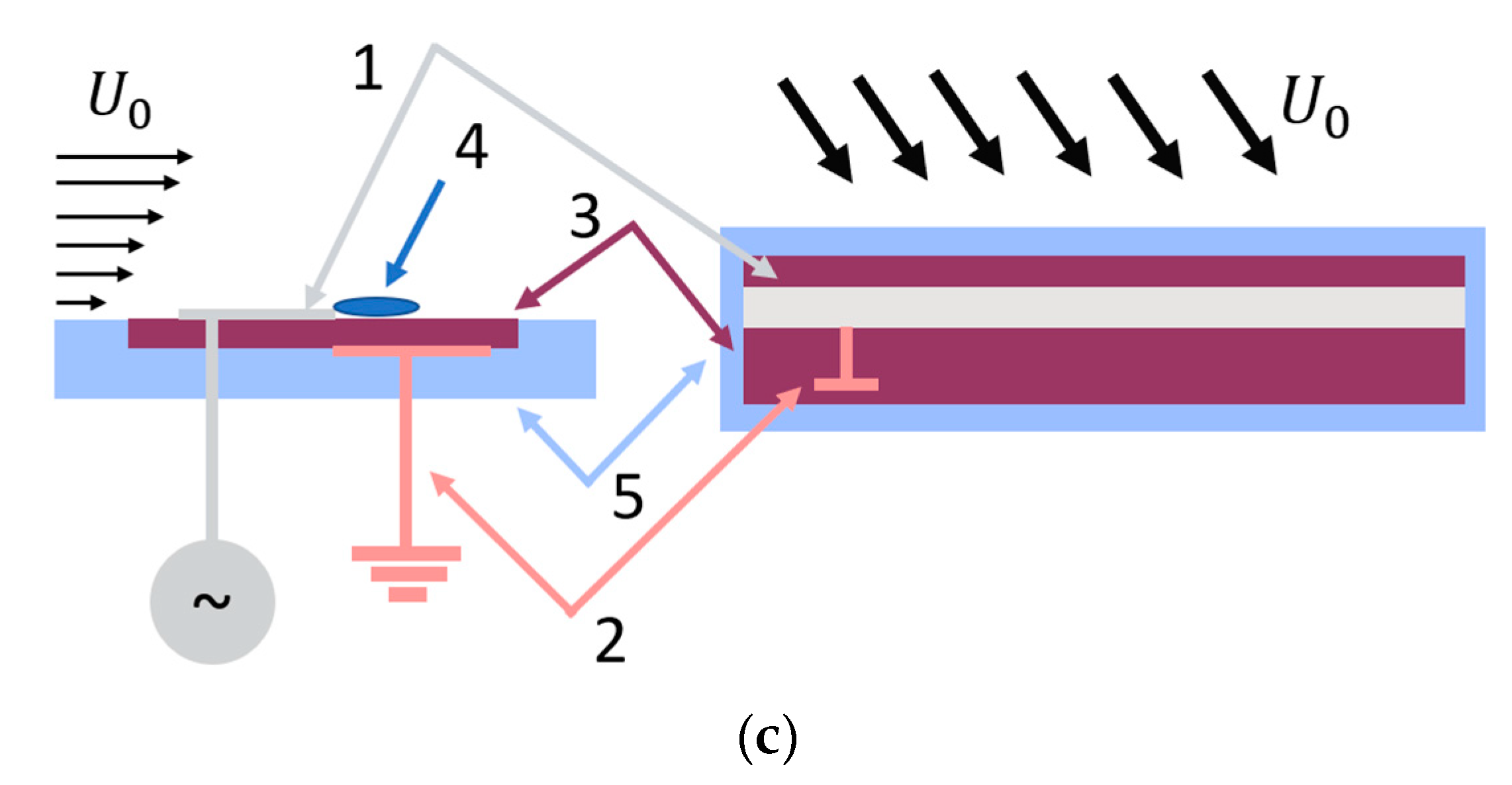
2.3.2. Actuator Model

In order to find the control perturbations induced by a single actuator section, its action on the flow was described by the volume force. Longitudinal $F_x$ and spanwise $F_y$ components of this force were described by the following analytical expressions

$$\begin{gathered} \left\{F_x,F_y\right\}=\epsilon \left\{f_x,f_y\right\}\left(x,y,z\right), \\ {f}_x=A\left(x\right)X\left(y\right)f\left(z\right), f_y=A\left(x\right)Y\left(y\right)f\left(z\right), f\left(z\right)=\frac{\overline{z}}{z_0}{e}^{-\overline{z}}, \\ X\left(y\right)=\frac{1}{2\surd \overline{2\pi }}\frac{1}{y_0}{e}^{-\raisebox{1ex}{${\overline{y}}^2$}\!\left/ \!\raisebox{-1ex}{$2 $}\right.}, Y\left(y\right)=\frac{1}{y_0}\overline{y}{e}^{-\left|\overline{y}\right|}. \end{gathered}$$

(14)

Here, $\epsilon$ is a small parameter characterizing the amplitude of volume force; $\overline{x}=x/x$₀, $\overline{y}=y/y$₀, $\overline{z}=z/z$₀, and $x_0$, $y_0$, $z_0$ are characteristic lengths of the force domain in longitudinal, spanwise and vertical directions. This model is based on the results of PIV measurements of the velocity field induced by an SDBD actuator with crossed electrodes in [30]. Smooth force distribution over the longitudinal co-ordinate A(x) that is convenient for the spectral PSE solution approach was introduced.

$$\begin{gathered} A\left(x\right)=\frac{1}{x_0}G\left(\overline{x}\right)e^{-\overline{x}}, G\left(\overline{x}\right)=0 for \overline{x}<0, \\ G\left(\overline{x}\right)=\frac{\sigma }{2\pi }\left. [1+sin\left(\frac{2\pi }{\sigma }(\overline{x}-\mathsf{\Delta }\right)\right] for-\mathsf{\Delta }<\overline{x}<\mathsf{\Delta }, \\ G\left(\overline{x}\right)=\frac{\sigma }{2\pi }+\overline{x}-\mathsf{\Delta } for \overline{x}>\mathsf{\Delta }. \end{gathered}$$

Here, $\sigma =8\mathsf{\Delta }$ and $\mathsf{\Delta }=0.25$ is the length of the smooth junction of the linear function $G\left(\overline{x}\right)=\overline{x}$ and $G\left(\overline{x}\right)=0$.

Fourier transforms of perturbations induced by the actuator section ${\tilde{u}}_{\tau a}$ at rather large distances downstream from it are also described by the solution of PSE with the proper amplitude.

$${\tilde{u}}_{\tau a}\left(\beta ,x\right)=a\left(\beta ,x\right){\tilde{u}}_{0\tau }\left(\beta ,x,z\right) ; {\tilde{u}}_0=\frac{\widetilde{u_{\tau }}\left(\beta ,x,z\right)e^{i\psi \left(\beta ,x\right)}}{\underset{z}{\max }\left(\widetilde{u_{\tau }}\left(\beta ,x,z\right)e^{i\psi \left(\beta ,x\right)}\right)}.$$

Here, ${\tilde{u}}_{\tau 0}$ is the solution of PSE normalized to obtain the unit amplitude at the distance x from the leading edge. This amplitude is found by solving the adjoint parabolic stability equations, with the solution sought in the form

$$\left\{u^{+},v^{+},w^{+},p^{+}\right\}\left(x,\beta ,z\right)=\left\{u_a^{+},v_a^{+},w_a^{+},p_a^{+}\right\}\left(\frac{x}{R}\right)e^{i{\psi }^{+}},$$

similar to (11).

These adjoint parabolized stability equations are integrated upstream starting from the eigenfunction of the adjoint Orr–Sommerfeld equation. Amplitude $a\left(\beta \right)$ can be found from the Green–Lagrange identity, which is derived by means of term-to-term scalar multiplication of linearized N-S equations to adjoin velocity components and pressure. This leads to the expression for amplitude in the form

$$a=\frac{{\int }_{-\mathsf{\Delta }}^{\mathsf{\Delta }}\left. [{\int }_0^{\infty }\left(u^{+*}\widetilde{F_x}+v^{+*}\widetilde{F_y}\right)dz\right]dx}{{\int }_0^{\infty }\left. [p^{+*}{u}_0+u^{+*}{p}_0+\left(U_0-i\frac{{\alpha }^{+*}+\alpha }{R}\right)\left(u^{+*}{u}_0+v^{+*}{v}_0+w^{+*}{w}_0\right)\right]\left(x_{r,}z\right)dz}.$$

(15)

Here, ${\alpha }^{+}=\frac{d{\psi }^{+}}{dx}$ is the adjoint longitudinal wavenumber. Limits of integration over x in the nominator of (15) should be large with respect to the longitudinal size of the body force region. A detailed description of this expression together with the derivation of adjoint PSE equations can be found in [33].

To compute the perturbations induced by the actuator section, the Fourier transforms of disturbances $\left\{\tilde{u},\tilde{v},\tilde{w},\tilde{p}\right\}$ were found in 51 grid points ${\beta }_n$, which were uniformly distributed in interval $\left. [0.1, 1.5\right]$. For each ${\beta }_n$, parabolized stability equations were integrated starting from eigenfunction found at streamwise co-ordinate $x_0=100$. Integration of PSE was finished at $x_{out}=1000,$ corresponding approximately to distance 400 mm downstream of the actuator. After this, adjoint PSE were integrated backward from $x_{out}$ to $x_0$, starting from the eigenfunction of the adjoint Orr–Sommerfeld equation. The solution in the physical space was found by means of Fourier integral (11) evaluation via the trapezoid method. The accuracy of computation of perturbations of streamwise velocity in the far field via this numerical method is estimated as 2% from its maximal value at the same distance from the discharge. The accuracy of finding this maximal amplitude is approximately the same.

3. Results and Discussion

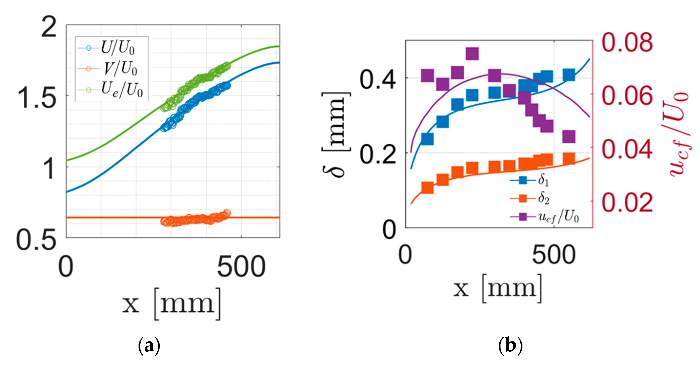
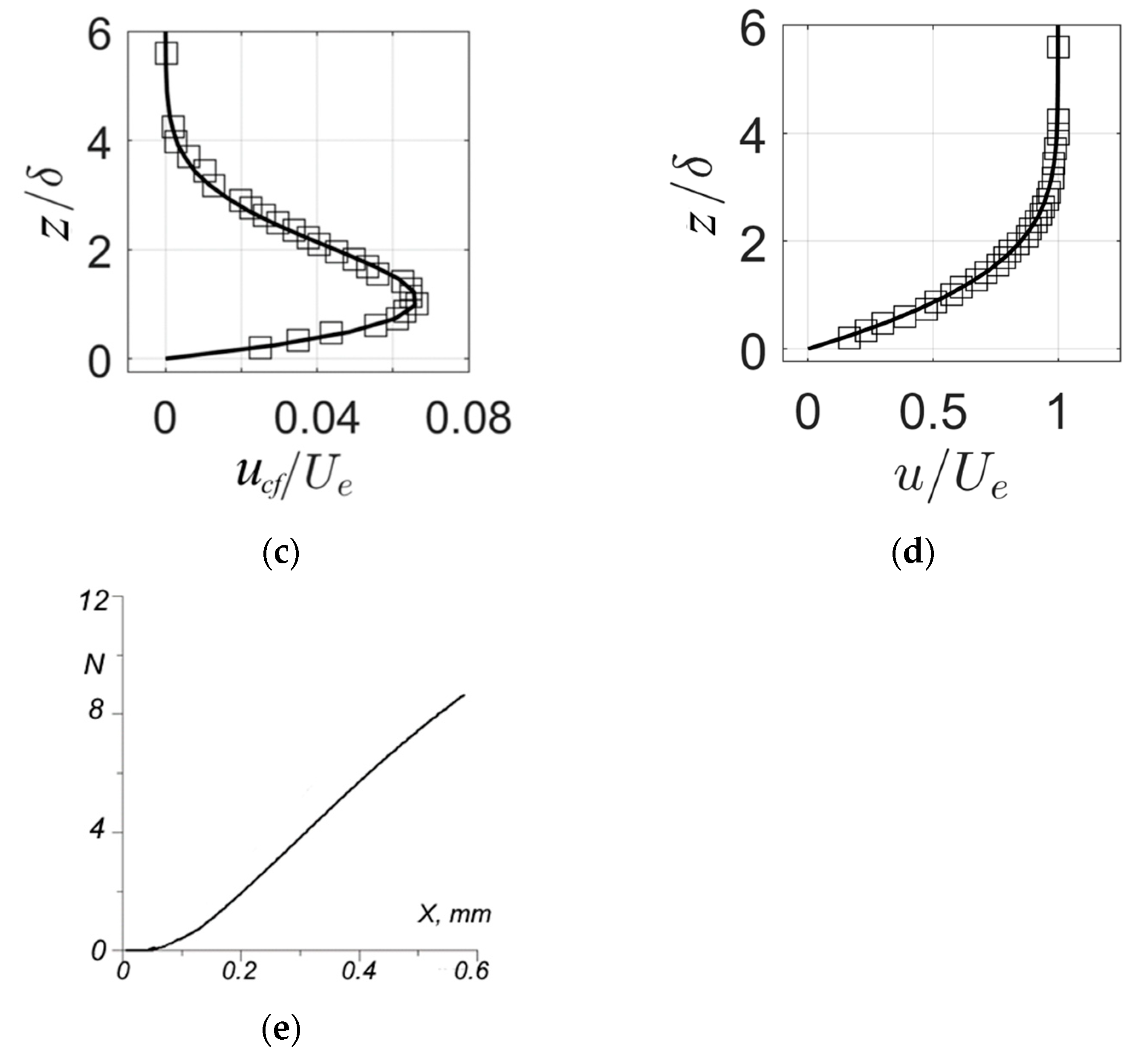
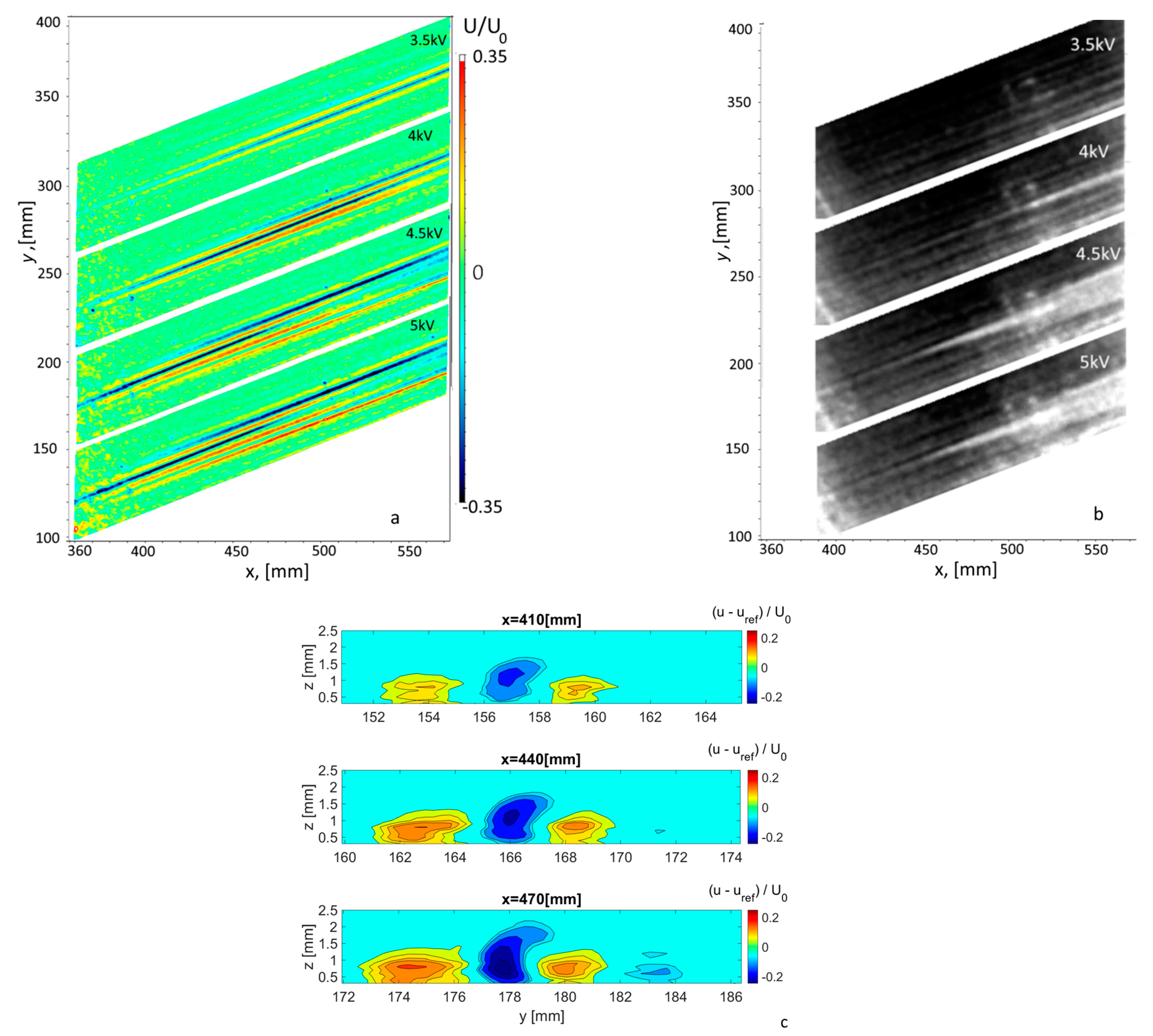
3.1. Boundary-Layer Excitation via Single Actuator Section

Boundary-layer response to the stationary localized forcing via the plasma actuator was measured as follows. A scan of the flow in the wall-normal direction was performed with a step of 0.1 mm. For each position, the in-plane velocity field was estimated both with actuation and for the reference case. It was assumed that within some distance to the actuator, the linear assumption is valid, and thus, the actuated flow is a superposition of the induced disturbances and natural ones. In this case, the BL response is calculated as $u_1\left(x,y,z\right)-u_{01}\left(x,y,z\right)$. Figure 4 shows two cross-sections of the flow: one is a plan view at the height approximately corresponding to the disturbance maximum; the other is in the cross-flow plane at $X=350 \mathrm{mm}$. The results are given at the increasing voltage applied to the actuator section.

One can see that the actuator creates a narrow set of CF vortices, inducing fringes of velocity defects and excess in the boundary layer. The number of fringes increases as one moves downstream. An increase in the applied voltage leads to an increase in the velocity modulation depth. As one moves downstream, disturbance magnitude increases up to typical values of 50% pk–pk of the local freestream velocity. At a certain position, the transition to turbulence occurs at the most intense gradient at the central part of the wavepacket that can be seen from the growth of short-wavelength perturbations (Figure 4b). The maximum of the disturbance magnitude is obtained at $z=0.7 \mathrm{mm}$ (Figure 3c), which corresponds to $1.5{\delta }^{*}$.

Linearity limits for the system were checked during voltage amplitude variation for the plasma actuator. Figure 3d shows transversal velocity profiles at the positions X = 400 mm and 450 mm. One can see that the disturbance structure remains conservative until the disturbance peak-to-peak magnitude reaches 5–7 m/s or 10–15% of U_e. For higher amplitudes, nonlinear saturation affects the measured shape of the transversal velocity profile. Above the voltage amplitude 5 kV, discharge filamentation occurs, which also alters the shape of the observed vortex packet. Below the modulation depth of 10%, the U_e boundary layer and actuator can be treated as a linear system, with the disturbance magnitude monotonically scaling with applied voltage and its structure remaining constant.

The structure of the discharge-induced disturbance, which is obtained from the numerical modeling, is shown in Figure 5. One can see that the overall structure of the wavepacket is remarkably similar to the experimental data. A detailed comparison (Figure 5b) shows that the main discrepancy comes from the trajectory of the disturbances in the boundary layer, which is probably due to the deviation of the model mean flow from the experimental one. Furthermore, as one moves downstream and at elevated forcing magnitudes, the disturbance structure is deformed due to nonlinear effects.

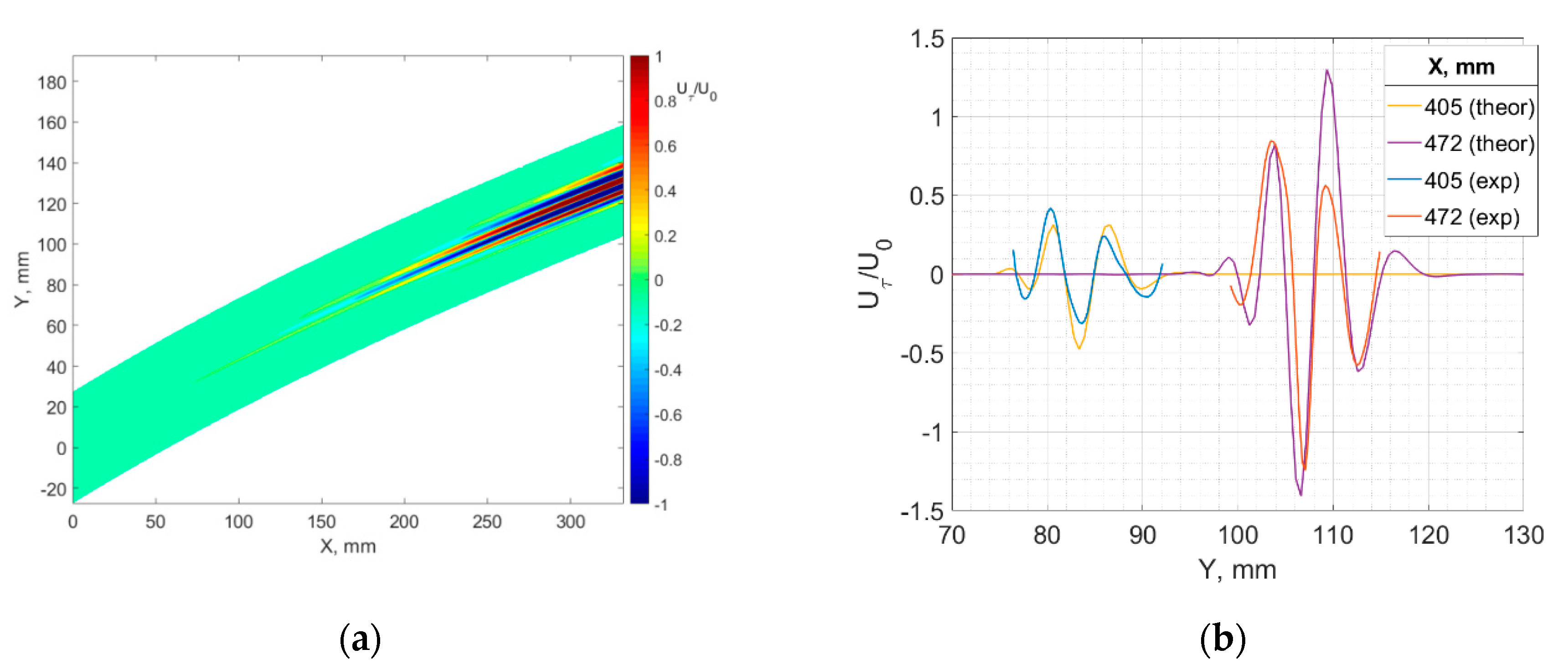
3.2. Modeling of Transition Control via Cross-Flow Vortex Cancellation

3.2.1. Control Simulation by Using Numerically Obtained Boundary-Layer Response

Natural disturbance was induced by random roughness at the position $x_0=61 \mathrm{mm}$. Control was performed by an actuator located at $x_a=100 \mathrm{mm}$ and reference section $x_c=305 \mathrm{mm}$. Results were averaged over a hundred realizations of the random roughness phase vector, according to (13).

Averaged RMS of the stationary disturbances was calculated for controlled and reference cases for actuator width $2b=25$ and 50 mm, with sections pitch $\Delta y~1.5 \mathrm{mm}$. Calculations were performed to find optimal control. Figure 6 shows that the control amplitude penalty decrease ε leads to the higher remaining vortex magnitude at the central part of the output cross-section; however, peaks are formed at its edges. From the tradeoff between edge effects and control efficiency in the central part of the span, $\mathsf{\epsilon }=0.01$ was determined as optimal, demonstrating up to a 50-times decrease in the amplitude of the initial signal. A comparison of two computations for wide and narrow control regions shows that the typical half-width of the edge region at $X=350 \mathrm{mm}$ is in the order of 7 mm. Thus, a narrow (25 mm) actuator with 17 sources allows efficient control only in the narrow region ~15 mm, although the efficiency of this control at the midspan remains unaffected.

The effect of the actuator resolution on the system performance is presented in Figure 7. It can be seen that the attainable reduction in the stationary vortices increases with a decrease in the pitch of the actuator array, until the value of Δy = 1.5 mm or 3.5–4 δ₁. This roughly corresponds to 4 actuators per critical disturbance period for the considered flow conditions.

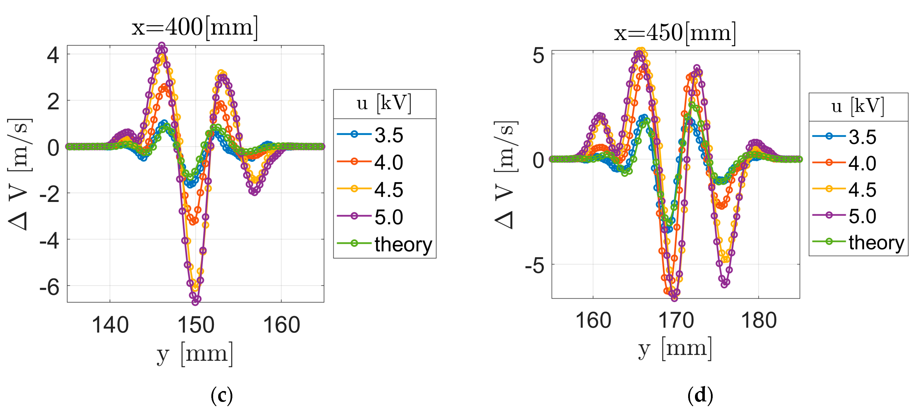
3.2.2. Control Simulation by Using Experimentally Obtained Boundary-Layer Response

Control simulation was performed for the set of actuators, which were installed with a fixed gap at X = 200 mm. The number of actuators was varied, q = 16, 32. The pitch of the actuator array was Δy = 1.5 mm to 2.1 mm, which roughly corresponds to 1/5 to 1/3 of the critical disturbance’s wavelength. The signal was minimized at distance X = 440 mm from the leading edge. All actuators are assumed to be equivalent; the experimentally observed response of the boundary layer to the single-channel excitation is taken to formulate the matrix $P$ in (5).

Optimal solutions, which are found from the two approaches, are shown in Figure 8. One can see that similar to the numeric estimation, a significant reduction in the CFI vortex amplitude can be obtained in the central part of the controlled span, and up to a five-times reduction in the signal RMS is obtained. At the edges of the controlled region, strong vortices are generated, induced by edge actuator sections. Linear regression with a further signal shift leads to higher edge effects, while the constrained optimal solution balances their magnitude and the performance in the central region. The requirement of u to be strictly positive leads to some deterioration of the control in the central section. Finally, one can see that for the CFI vortices created by random roughness, minimization of the signal RMS ($n_2$) also leads to a comparable reduction in the signal peak-to-peak amplitude ($n_{inf}$).

Modelling of the CF vortex cancellation with a real experimentally observed response demonstrates a not-so-dramatic effect in comparison to the numeric case. It can be speculated that the reason is the somehow different spectral composition of the disturbances, the presence of bias errors in velocity distribution in the experimental data or different positions of the plasma actuator.

Assuming linear superposition of the natural and actuator-induced vortices, we can model the velocity distribution in the boundary layer. Figure 9 shows the simulated results for various approaches that are used for the optimal control evaluation. One can see that although the control quality decreases as we move downstream, vortex amplitude reduction is obtained along a substantial part of the chord.

Finally, we can roughly estimate the energetic efficiency of the method proposed for the given experimental conditions. Assuming the friction coefficient in a turbulent boundary layer to be C_ft ~ 5 × 10⁻³, we obtain the local friction for 40 m/s to be ${\tau }_w=5.2 \mathrm{N}/{\mathrm{m}}^2$ and the skin friction power losses to be $P_f=210 \mathrm{W}$. For laminar flow, we take the value C_fl ~ 1 × 10⁻³. Stability estimates (Figure 2e) for a given boundary layer show that a ten-times increase for the stationary CF vortex magnitude occurs within 120 mm along the streamwise co-ordinate. If a transition occurs at a fixed disturbance magnitude, 20 dB reduction can be recalculated to an approximately $∆X_t=150 \mathrm{mm}$ shift of the transition line. That is, for the given conditions, the energy saving due to flow laminarization will be $∆C_{f}0.5 \rho U_e^3 ∆X_t=25 \mathrm{W}$. The estimated power consumption for the plasma actuator, based on its resolution and energy input 0.17 W/section, is 113 W/m. For the conditions of the present experiment, efficiency will be η = 22%. One should note that this value is based on a rough estimation of the friction coefficient, which was made for a zero-pressure gradient boundary layer and not taking into account modulation of the flow by cross-flow vortices. Finally, this estimate does not take into account the nonlinear stage of disturbances development, which has a considerable length for the swept-wing boundary layer.

Vortex cancellation can be compared with the other approaches considered for flow laminarization by using plasma actuators. The total thrust induced by the actuator is 1.6 mN/m. Introducing the momentum coefficient as $C_{\mu }=F_x/\left(0.5\rho U_e^2{\delta }_1\right)$, we obtain, for the quantities U_e and δ₁ taken at the actuator position, $C_{\mu }=0.005$. For the base flow modification strategy, when the cross-flow velocity profile is altered by the actuator, authors of [16,34] obtain an approximately 50 mm (4% chord) transition shift at $C_{\mu }~0.2-0.5$. Similar in the order, the results are obtained when the boundary layer is controlled by a subcritical “plasma roughness” from the leading edge.

Thus, the vortex cancellation approach should demonstrate a superior efficiency compared to the base flow modification technique. Still, to obtain energetic efficiency above unity, further optimization of the method will be required.

4. Conclusions

Plasma actuators with a limited discharge span can be used to force the isolated stationary cross-flow vortex packets in a boundary layer. The disturbance structure in the asymptotic region is well predicted by PSE calculations, with discharge modelled by a 2-component force domain.

At peak-to-peak disturbance amplitudes <10%, the boundary layer and the actuator are treated as a linear system. System identification can be performed by measuring or calculating the boundary-layer asymptotic response to a single section excitation via step function.

The optimal control strategy is proposed for CFI vortex cancellation, based on the response function of the boundary layer and measured uncontrolled system output. Since the admissible control is limited to positive values, the quadratic cost function optimization with constraint is used to find a solution. Alternatively, high control quality can be achieved in the central part of the span by solving the unconstrained linear regression problem and shifting the result by a fixed value to achieve strictly positive control. The latter approach appears to be faster, despite exciting strong vortices at the edges of the controlled region.

An evaluation of these algorithms was performed based on simulated boundary-layer response and simulated natural disturbances introduced near the leading edge, and both quantities obtained from the experiment. A decrease in the spanwise velocity RMS up to 50 times and up to 5 times was obtained for these two cases, respectively. Minimum actuator resolution, providing adequate results, corresponds to ¼ of the spanwise wavelength estimated for the most growing cross-flow vortices, or 1.5 mm (3–4 δ₁) for the conditions of present study. The analysis presented is linear and, thus, applies only to the disturbances with amplitude less than 10–15% of local flow velocity. For higher magnitudes, the proposed approach can give suboptimal results; nonlinear optimization strategies can demonstrate higher efficiency. Moreover, heat release effects were not taken into account in this study. For higher flow velocity, they can also contribute to the excitation of the cross-flow modes. Moreover, average flow heating was not taken into account, although it can slightly affect boundary-layer stability in certain conditions [35].

References

1. Bippes, H. Basic Experiments on Transition in Three-Dimensional Boundary Layers Dominated by Crossflow Instability. Prog. Aerosp. Sci. 1999, 35, 363–412. [Google Scholar] [CrossRef]
2. Saric, W.S.; Reed, H.L.; White, E.B. Stability and transition of Three-dimensional boundary layers. Annu. Rev. Fluid Mech. 2003, 35, 413–440. [Google Scholar] [CrossRef]
3. Borodulin, V.I.; Ivanov, A.V.; Kachanov, Y.S. Swept-wing boundary-layer transition at various external perturbations: Scenarios, criteria, and problems of prediction. Phys. Fluids 2017, 29, 094101. [Google Scholar] [CrossRef]
4. Ustinov, M.V. Laminar-turbulent transition in boundary layers (Review). Part 1: Main types of laminar-turbulent transition in a swept-wing boundary layer. TsAGI Sci. J. 2013, 44, 1–63. [Google Scholar] [CrossRef]
5. Ustinov, M.V. Laminar-turbulent transition in boundary layers (Review). Part 1: Transition prediction and methods of boundary layer laminarization. TsAGI Sci. J. 2014, 45, 851–887. [Google Scholar] [CrossRef]
6. Thomas, A.S.W. The control of boundary-layer transition using a wave-superposition principle. J. Fluid Mech. 1983, 137, 233–250. [Google Scholar] [CrossRef]
7. Ladd, D.M.; Hendricks, E.W. Active control of 2-D instability waves on an axisymmetric body. Exp. Fluids 1988, 6, 69–70. [Google Scholar] [CrossRef]
8. Li, Y.; Gaster, M. Active control of boundary-layer instabilities. J. Fluid Mech. 2006, 550, 185–205. [Google Scholar] [CrossRef]
9. Sturzebecher, D.; Nitsche, W. Active cancellation of Tollmien–Schlichting instabilities on a wing using multi-channel sensor actuator systems. Int. J. Heat Fluid Flow 2003, 24, 572–583. [Google Scholar] [CrossRef]
10. Zoppini, G.; Michelis, T.; Ragni, D.; Kotsonis, M. Cancellation of crossflow instabilities through multiple discrete roughness elements forcing. Phys. Rev. Fluids 2022, 7, 123902. [Google Scholar] [CrossRef]
11. Moreau, E. Airflow control by non-thermal plasma actuators. J. Phys. D Appl. Phys. 2007, 40, 605–636. [Google Scholar] [CrossRef]
12. Kriegseis, J.; Simon, B.; Grundmann, S. Towards In-Flight Applications? A Review on Dielectric Barrier Discharge-Based Boundary-Layer Control. Appl. Mech. Rev. 2016, 68, 020802. [Google Scholar] [CrossRef]
13. Wang, J.-J.; Choi, K.-S.; Feng, L.-H.; Jukes, T.N.; Whalley, R.D. Recent developments in DBD plasma flow control. Prog. Aerosp. Sci. 2013, 62, 52–78. [Google Scholar] [CrossRef]
14. Samimy, M.; Webb, N.; Esfahani, A. Reinventing the wheel: Excitation of flow instabilities for active flow control using plasma actuators. J. Phys. D: Appl. Phys. 2019, 52, 354002. [Google Scholar] [CrossRef]
15. Baranov, S.A.; Kiselev, A.F.; Kuryachii, A.P.; Sboev, D.S.; Tolkachev, S.N.; Chernyshev, S.L. Control of Cross-Flow in a Three-Dimensional Boundary Layer Using a Multidischarge Actuator System. Fluid Dyn. 2021, 56, 66–78. [Google Scholar] [CrossRef]
16. Yadala, S.; Hehner, M.T.; Serpieri, J.; Benard, N.; Kotsonis, M. Plasma-Based Forcing Strategies for Control of Crossflow Instabilities. AIAA J. 2021, 59, 3406–3416. [Google Scholar] [CrossRef]
17. Chernyshov, S.L.; Kuriachii, A.P.; Manuilovich, S.V.; Russianov, D.A.; Gamirullin, M.P. Theoretical Modeling of the Electrogasdynamic Method of Laminar Flow Control on a Swept Wing. In Proceedings of the 9th Congress of the International Council of Aeronautical Sciences, St. Petersburg, Russia, 7–12 September 2014. [Google Scholar]
18. Kuryachii, A.P. Control of cross flow in the three-dimensional boundary layer using space-periodic body force action. Fluid Dyn. 2009, 44, 233–239. [Google Scholar] [CrossRef]
19. Duchmann, A.; Simon, B.; Magin, P.; Tropea, C.; Grundmann, S. In-Flight Transition Delay with DBD Plasma Actuators. In Proceedings of the 51st AIAA Aerospace Sciences Meeting including the New Horizons Forum and Aerospace Exposition, Grapevine, TX, USA, 7–10 January 2013. [Google Scholar] [CrossRef]
20. Serpieri, J.; Venkata, S.Y.; Kotsonis, M. Conditioning of cross-flow instability modes using dielectric barrier discharge plasma actuators. J. Fluid Mech. 2017, 833, 164–205. [Google Scholar] [CrossRef]
21. Baranov, S.; Moralev, I.; Ustinov, M.; Sboev, D.; Tolkachev, S. Transition Control by Dielectric Barrier Discharge in a Swept Wing Boundary Layer at Elevated Free Stream Turbulence. In Proceedings of the 593 Euromech Colloqium “PLASMA-BASED ACTUATORS FOR FLOW CONTROL: RECENT DEVELOPMENTS AND FUTURE DIRECTIONS”, Delft, The Netherlands, 14–16 March 2018. [Google Scholar]
22. Choi, K.-S.; Kim, J.-H. Plasma virtual roughness elements for cross-flow instability control. Exp. Fluids 2018, 59, 1–15. [Google Scholar] [CrossRef]
23. Moralev, I.; Ustinov, M.; Kotvitskii, A.; Popov, I.; Selivonin, I.; Kazanskii, P. Stochastic disturbances, induced by plasma actuator in a flat plate boundary layer. Phys. Fluids 2022, 34, 054117. [Google Scholar] [CrossRef]
24. Moralev, I.; Selivonin, I.; Ustinov, M. On the stochastic forcing of the boundary layer by plasma actuators. Exp. Fluids 2019, 60, 177. [Google Scholar] [CrossRef]
25. Baranov, S.A.; Kiselev, A.P.; Moralev, I.A.; Sboev, D.S.; Tolkachev, S.N.; Chernyshev, S.L. Transition control in a three-dimensional boundary layer at elevated free stream turbulence using dielectric barrier discharge. Dokl. Phys. 2019, 486, 668–672, In Russian. [Google Scholar] [CrossRef]
26. Dörr, P.; Kloker, M. Transition control in a three-dimensional boundary layer by direct attenuation of nonlinear crossflow vortices using plasma actuators. Int. J. Heat Fluid Flow 2016, 61, 449–465. [Google Scholar] [CrossRef]
27. Moralev, I.; Selivonin, I.; Tatarenkova, D.; Firsov, A.; Preobrazhenskii, D. Damping of the longitudinal streak in the boundary layer by ‘plasma panel’ actuator. J. Phys. D Appl. Phys. 2019, 52, 304003. [Google Scholar] [CrossRef]
28. Manuilovich, S.V. Bulk forces removing the cross-flow in the laminar boundary layer. Fluid Dyn. 2000, 15, 387–397. [Google Scholar]
29. Selivonin, I.; Lazukin, A.; Moralev, I.; Krivov, S. Effect of electrode degradation on the electrical characteristics of surface dielectric barrier discharge. Plasma Sources Sci. Technol. 2018, 27, 085003. [Google Scholar] [CrossRef]
30. Moralev, I.; Bityurin, V.; Firsov, A.; Sherbakova, V.; Selivonin, I.; Maxim, U. Localized micro-discharges group dielectric barrier discharge vortex generators: Disturbances source for active transition control. Proc. Inst. Mech. Eng. Part G J. Aerosp. Eng. 2020, 234, 42–57. [Google Scholar] [CrossRef]
31. Bertolotti, F.P.; Herbert, T.; Spalart, P.R. Linear and non-linear stability of the Blasius boundary layer. J. Fluid Mech. 1992, 242, 441–474. [Google Scholar] [CrossRef]
32. Li, F.; Malik, M.R. On the Nature of PSE Approximation. Theor. Comput. Fluid Dyn. 1996, 8, 253–273. [Google Scholar] [CrossRef]
33. Airiau, C. Non-Parallel Acoustic Receptivity of a Blasius Boundary Layer Using an Adjoint Approach. Flow, Turbul. Combust. 2000, 65, 347–367. [Google Scholar] [CrossRef]
34. Yadala, S.; Hehner, M.T.; Serpieri, J.; Benard, N.; Dörr, P.C.; Kloker, M.J.; Kotsonis, M. Experimental control of swept-wing transition through base-flow modification by plasma actuators. J. Fluid Mech. 2018, 844, R2. [Google Scholar] [CrossRef]
35. Hui, W.; Zhang, H.; Wang, J.; Meng, X.; Li, H. Heat transfer characteristics of plasma actuation in different boundary-layer flows. Phys. Fluids 2022, 34, 034110. [Google Scholar] [CrossRef]
Figure 1. (a) Test section and 2D PIV scheme: 1—curvilinear test section, 2—swept plate, 3—laser sheet, 4—camera. (b) Co-ordinates system and location of plasma actuator: 1—single-section plasma actuator, 2—laser sheet, 3—swept plate. (c) Principal scheme of single-section plasma actuator: 1—high voltage electrode, 2—ground electrode, 3—ceramic, 4—plasma, 5—panel.
Aerospace 10 00469 g001aAerospace 10 00469 g001b
Figure 2. (a) Mean flow components. (b) Boundary-layer parameters. (c) Cross-flow velocity profile. (d) Streamline velocity profile. (e) N factors, obtained for the stationary disturbances with critical wavelength 6.8 mm. Symbols correspond to experimental data, and lines correspond to calculations.
Aerospace 10 00469 g002aAerospace 10 00469 g002b
Figure 3. Sketch of system control.
Aerospace 10 00469 g003
Figure 4. Asymptotic response of the boundary-layer-to-step excitation by a single section of plasma actuator. (a) In-plane velocity distribution. (b) Transition visualization by short-wavelength disturbances magnitude. (c) Disturbances structure in the cross-flow plane.
Aerospace 10 00469 g004
Figure 5. (a) Calculated response of the boundary layer. (b) Comparison between theory and experiment at several streamwise positions. (c,d) Velocity profiles for various voltage amplitude.
Aerospace 10 00469 g005aAerospace 10 00469 g005b
Figure 6. Ensemble-averaged spanwise velocity distributions. (a) For q = 32, b = 50 mm. (b) For q = 16, b = 25 mm. The dotted line corresponds to the reference case (boundary layer, perturbed by random roughness).
Aerospace 10 00469 g006
Figure 7. Effect of actuator resolution (pitch of actuator array) on the control quality.
Aerospace 10 00469 g007
Figure 8. Modeling of the cross-flow vortex cancellation, which is based on experimentally observed reference and boundary-layer response. (a) Δ y = 2.1   mm ; (b) Δ y = 1.8   mm ; (c) Δ y = 1.5   mm . u r e g . —solution of linear regression problem, u r e g . o f f s e t —shifted vector u r e g . , u o p t —solution of constrained optimization problem.
Aerospace 10 00469 g008
Figure 9. Linear simulation of the cross-flow vortices control in the boundary layer.
Aerospace 10 00469 g009
Disclaimer/Publisher’s Note: The statements, opinions and data contained in all publications are solely those of the individual author(s) and contributor(s) and not of MDPI and/or the editor(s). MDPI and/or the editor(s) disclaim responsibility for any injury to people or property resulting from any ideas, methods, instructions or products referred to in the content.