1. Introduction
The first mission targeting a small body dates back to 1996 when NASA’s Near Earth Asteroid Rendezvous (NEAR-Shoemaker) concluded the first non-incidental close rendezvous with asteroid (253) Mathilde. NEAR-Shoemaker also achieved the first soft landing on (433) Eros’ surface in 2001 [
1]. From that moment, close-proximity operations (CPOs) around small bodies have emerged as a relevant topic in space exploration. However, CPOs are non-trivial activities for spacecraft targeting small bodies. Indeed, the need for high accuracy in a risky environment, combined with the short time available for operations, makes CPOs challenging from both a conceptual and a technological point of view. A certain degree of autonomy or a strong effort from ground operators were the strategies used in the past to achieve a successful rendezvous. In Hayabusa 1 [
2] and Hayabusa 2 [
3], two recent successful missions to asteroids, sample operations were conducted autonomously by the probes, while critical operations for ESA’s Rosetta mission required a timely dedication by the on-ground flight dynamics team [
4]. Recently, an increasing number of space exploration mission concepts foresee the exploitation of CubeSats [
5]. The two MARCO [
6] CubeSats were the first, while in the near future there will be missions targeting asteroids such as M-ARGO [
7], NEA SCOUT [
8] and the two Hera CubeSats, Milani [
9] and Juventas [
10]. Thus, understanding the real capabilities of low-cost nanosatellites that operate close to a small body is of great interest.
However, overcoming the technological challenges posed by CPO is not always possible when low-cost solutions, such as CubeSats, are employed, and the strategies developed for traditional spacecraft may not be suitable for small platforms. Novel navigation techniques or the lack of a dedicated full-time on-ground team, related to the low-cost nature of CubeSats, can increase the uncertainties in the state observation. In addition, the performance and accuracy of miniaturized components (e.g., thruster magnitude and pointing uncertainty) are often not comparable to standard ones due to their lower maturity. Consequently, theoretical trajectories might become unfeasible when real-world constraints are considered, and, while for traditional spacecraft missions, consideration of the uncertainties and ground constraints could generally be made a posteriori, when working with CubeSats flying in complex environments, the trajectory design should include them even in the preliminary stages. When considering highly perturbed environments and low-cost solutions such as CubeSats, it must be clear that a navigation assessment to check for the flyability of the trajectories is essential.
In this work, an alternative approach to the trajectory design pipeline for CubeSats during CPO is presented. This work is not focused on the dynamical analysis or on the trajectory generation, which have been well investigated in [
11]. Its aim is rather to show the importance/influence of operative constraints and dynamical uncertainties on the trajectory design. This is approach has been successfully applied in the Hera Milani CubeSat mission analysis, here presented as a test case.
This paper is structured as follows:
Section 2 introduces the Milani mission. The dynamical environment is detailed and the vehicle is presented.
Section 3 shows the trajectory-design constraints, strategy and results, while
Section 4 is focused on navigation assessment. Finally, in
Section 5 a conclusion and critical assessment are presented.
2. The Milani Mission
The Milani mission, named after the mathematician Andrea Milani (
https://www.esa.int/Space_in_Member_States/Italy/Andrea_Milani_1948_2018 (last accessed 1 March 2023)), is framed within the Hera mission of the European Space Agency (ESA). Hera is the ESA part of the AIDA (Asteroid Impact and Deflection Assessment) [
12] international collaboration with NASA, which is responsible for DART (Double Asteroid Redirection Test) [
13]. Hera and DART have been conceived to be mutually independent. However, their value is increased when combined. The target of the Hera mission is the (65803) Didymos binary asteroid, which was impacted by DART on 27 September 2022. Following the impact, a crater was likely created on the secondary asteroid, Dimorphos. Hera will rendezvous with the asteroid in January 2027 carrying two CubeSats as opportunistic payloads, Juventas and Milani. Milani is scheduled to be released in March 2027 in proximity to the system. The main scientific goals of Milani are (1) to obtain a detailed mapping and characterization of the asteroids and (2) to characterize the dust environment around them. The CubeSat will achieve these goals during the two main scientific phases: the far-range phase (FRP) and the close-range phase (CRP) [
14]. After the deployment from Hera, Milani will start to observe the asteroid at around 10 km during FRP. After 1 month of observations, Milani will move closer during the CRP to observe Dimorphos at higher resolutions. At the end of the CRP, Milani will be injected into a Sun-synchronous terminator orbit (SSTO) and will attempt a landing on Dimorphos. This work focuses on the challenging solutions found for the CRP, in which Milani needs to be less than 2 km away from the system to obtain high-resolution and well-illuminated images of the DART crater on Dimorphos.
2.1. Dynamical Environment
Didymos is a binary near-earth asteroid (NEA) of S-type, discovered in 1996, formed by Didymos, or D1 (the primary), and Dimorphos, or D2 (the secondary). In the reference model [
11], Dimorphos and Didymos are assumed to share the same equatorial plane on which their relative motion occurs. Dimorphos is assumed to be in a tidally locked configuration with Didymos. The latter assumption can be relevant when observing some features on the secondary, such as the crater created by the DART impact, since it would be illuminated and visible only at certain geometries.
Considering the point-mass model for both asteroids, the equation of motion for Milani in the quasi-inertial DydimosEclipJ2000 [
11] reference frame, centered at the barycenter of the binary system and having the axes
X and
Y lying on the ecliptic plane at epoch J2000 and the axis
Z orthogonal to this plane, can be written as
where
is the CubeSat position,
and
are the standard gravitational parameters of the primary and the secondary asteroid, respectively, while
and
are the CubeSat’s relative position with respect to the respective asteroids. The fourth-body effect due to the Sun can be written as
where
and
are the gravitational constants of the Sun and the whole Didymos system, respectively, and
is the position vector of the Sun.
The contribution the solar radiation pressure (SRP), which pushes the CubeSat away from the Sun, is computed using an SRP cannonball model [
15]:
where
is the solar flux at 1 AU,
c is the speed of light,
is the Sun–Earth distance,
is the reflectivity coefficient of the CubeSat,
A is its equivalent surface area and
M is its mass.
Table 1 summarizes the main parameters considered in the dynamics.
2.2. The Spacecraft
Milani is a 6U XL CubeSat, having a wet mass of about 12 kg and equipped with a cold-gas propulsion system for orbital maneuvers. Milani’s sensor suite is made of two Sun sensors, a star tracker, an IMU, a LIDAR and a navigation camera (NavCam) [
16]. As part of Milani technological goals, the CubeSat has to exchange information and communicate with Hera via an inter-satellite link (ISL). This instrument also provides information on the range and range-rate with respect to Hera. Thus, Milani’s optical navigation will also be supported by ISL measurements. The ISL antenna is omnidirectional and no eclipses with the body are foreseen during Hera’s motion. Thus, Hera’s visibility is always guaranteed.
Milani’s platform accommodates three scientific payloads: the ISL, VISTA [
17] and ASPECT [
18]. Among these, ASPECT is the most demanding from the trajectory-design point of view. ASPECT is a passive payload equipped with a visible to near-infrared hyperspectral imager, which will be used to perform global mapping of the asteroids with detailed observations of the DART crater on Dimorphos. Milani’s trajectories have been designed considering mainly the ASPECT goals for both the scientific phases. In particular, during the close approach in CRP, Milani needs to image Dimorphos with a spatial resolution better than 1 m/pixel and observe the DART crater with a spatial resolution better than 0.5 m/pixel at a phase angle (Sun–Asteroid–Milani angle) once at [0–10] deg and once at [30–60] deg. The requirements on the phase angle are the most challenging and they are the main drivers for the CRP design, while the mapping of whole the body will be a by-product of the crater-observation arc design. Indeed, 0.5 m/pixel translates into a desired distance of 2780 m from D2.
Table 2 summarizes the requirements for the observation windows, while
Figure 1 shows graphically the observation locations.
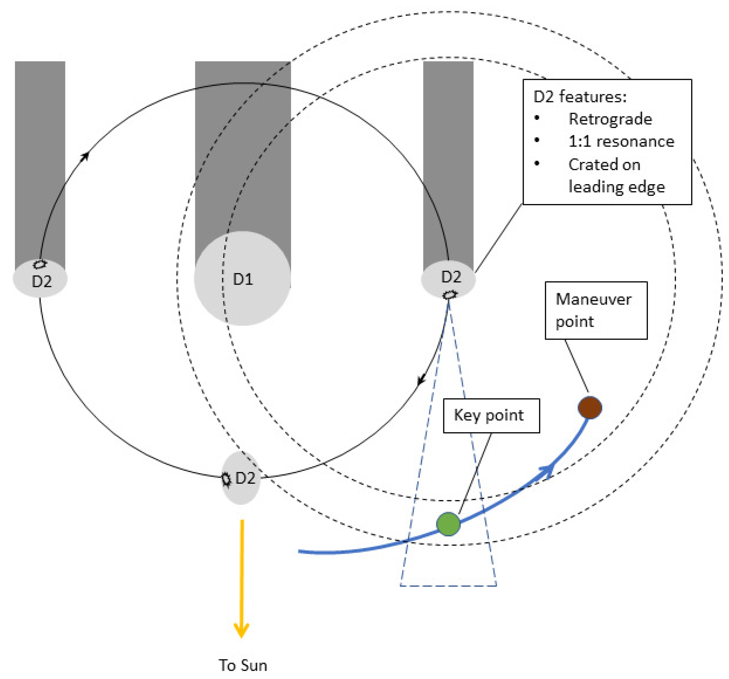
The requirement of the phase angle of [0–10] deg is particularly stringent when combined with the tidally locked nature of the system. Indeed, the relative motion of the system forces Milani to image the crater only when approaching the system and not when leaving it. Furthermore, the geometry of the system forces the CubeSat to maneuver shortly after the scientific acquisition to avoid going into the night side. Therefore, considering that a certain amount of time is required to prepare the orbital maneuvers, the time window available for scientific acquisitions is very limited.
3. Trajectory Options
Milani’s trajectory design has been driven by the main scientific goals of the mission and influenced by both technical and operational constraints. Two trajectory options are shown in the remainder. Their design process is out of the scope of this document and can be found in [
11,
14]. In this section, only the rationale behind them is presented, while further analyses are discussed in
Section 4.
3.1. Payload and Ground Constraints
An important constraint on the design space is introduced by the passive nature of ASPECT and the NavCam. As a consequence, Milani must fly on the day side of the system to perform both scientific observations and optical navigation. Therefore, the CubeSat needs to maneuver frequently to avoid going into the night side (i.e., where the phase angle is larger than 90 deg), performing a repetition of hovering legs that span the day-side region back and forth. Although having a high maneuvering frequency can be costly, it might be desirable in response to highly nonlinear dynamical environments or to scientific needs, but having a daily or hourly maneuvering schedule is unrealistic from an operational point of view. The need to maneuver frequently, i.e., with a temporal separation of a few hours or a day, is in contrast with the operational constraints associated with commanding the CubeSat from the ground. The time needed to perform the orbit determination and to prepare the correction maneuvers and the working schedule of the operative centers cannot ensure daily maneuvering, if not occasionally.
Hence, the turn-around time (TAT), i.e., the duration between the last navigation observable and the command uplink, has to be identified. In the case of Milani, the CubeSat can communicate with the ground only by using Hera as a relay. Thus, the TAT is actually the time elapsed from the instant Hera downlinks the observables to the moment Hera receives the telecommands obtained after all on-ground operations are completed. In order to avoid an open-loop command, no ballistic arc with a duration lower than the TAT can be designed if the ground is in the maneuvering loop.
Another constraint is given by the operative centers’ working schedule, since it is preferred to have repetitive operations with a weekly routine, avoiding critical events to happen during weekends or holidays. These details are particularly important when working on spacecraft missions around multiple small bodies, when phasing with the bodies is needed.
Since Hera acts as a relay for communication of Milani with the ground, in order to exploit the same Hera communication windows, the OD of Milani should be performed simultaneously with that of Hera; thus, the same TAT has to be considered for the two spacecraft. Hera’s flight dynamics team has considered a TAT of 48 h, which has then become the baseline for Milani. Therefore, the minimum possible duration for the CubeSat’s ballistic arcs is 48 h. For the same reason, Milani’s maneuvering schedule should be aligned with that of Hera. Thus, an additional constraint on the maneuvering schedule and frequency has to be considered since Milani should maneuver every 3 and 4 days, following the Hera schedule.
Table 3 summarizes the constraints for Milani trajectory design.
3.2. Waypoints and Keypoints
Previous work investigated trajectory options around Didymos for a CubeSat [
11] and showed early-phase trajectories for Milani [
19]. From these studies, the best design strategy for FRP observations (10 km) was the waypoints strategy.
The waypoint strategy is based on the selection of waypoints, which act as maneuver points between patched ballistic arcs. The geometry of the waypoints can be designed to fulfill the scientific requirements and meet the mission constraints as well, as seen with the Rosetta spacecraft about comet 67P/Churyumov–Gerasimenko [
4]. A simple waypoints strategy has been used to design Milani’s FRP, resulting in a repetition of hyperbolic orbits quasi-symmetric to the Sun direction [
11]. The Milani FRP’s main goal is to image the asteroids at a low phase angle at around 10 km of distance. Thus, the FRP is designed to maximize the time spent in those regions and so the possible scientific observations. By placing the waypoints as far as possible at the boundaries of the day side of the system, the spacecraft is forced to cover the largest distance possible in the time fixed by the constraints. By doing that, the trajectory found is fast enough to reach the desired range when passing through the low-phase-angle region. Therefore, the relative waypoint placement can control the minimum range reached during the arc. Unfortunately, this strategy is not suitable to fulfill the more challenging resolution requirements for CRP. Indeed, due to the constraints on the maneuvering frequency described before, which impose a minimum arc duration of 3 days (dictated by Hera), the minimum distance that can be reached with this strategy is 7 km, which is not sufficient to achieve the desired image resolution. To approach closer to the system, the solution introduced is to modify the waypoints strategy with the introduction of keypoints [
9]. A keypoint is a location where the spacecraft can perform the desired scientific observation while fulfilling all the scientific requirements. Differently from the waypoints, no maneuvers occur at a keypoint. Thus, the design focus moves from the maneuver point geometry to the definition of the keypoints, one for each crater measurement.
Figure 1 shows the keypoint design for the crater observations under the resolution and phase-angle requirements described in
Section 2.2. Consequently, the design of the maneuvers performed after the observations at the keypoints is performed only to avoid going into the night side. The resulting trajectory appears strongly asymmetrical, in contrast with the previous scientific phase.
3.3. CRP Trajectory Solutions
Two solutions for the Milani CRP, labeled for convenience “Option A” and “Option B”, have been designed and are discussed in the remainder of this section.
3.3.1. CRP—Option A
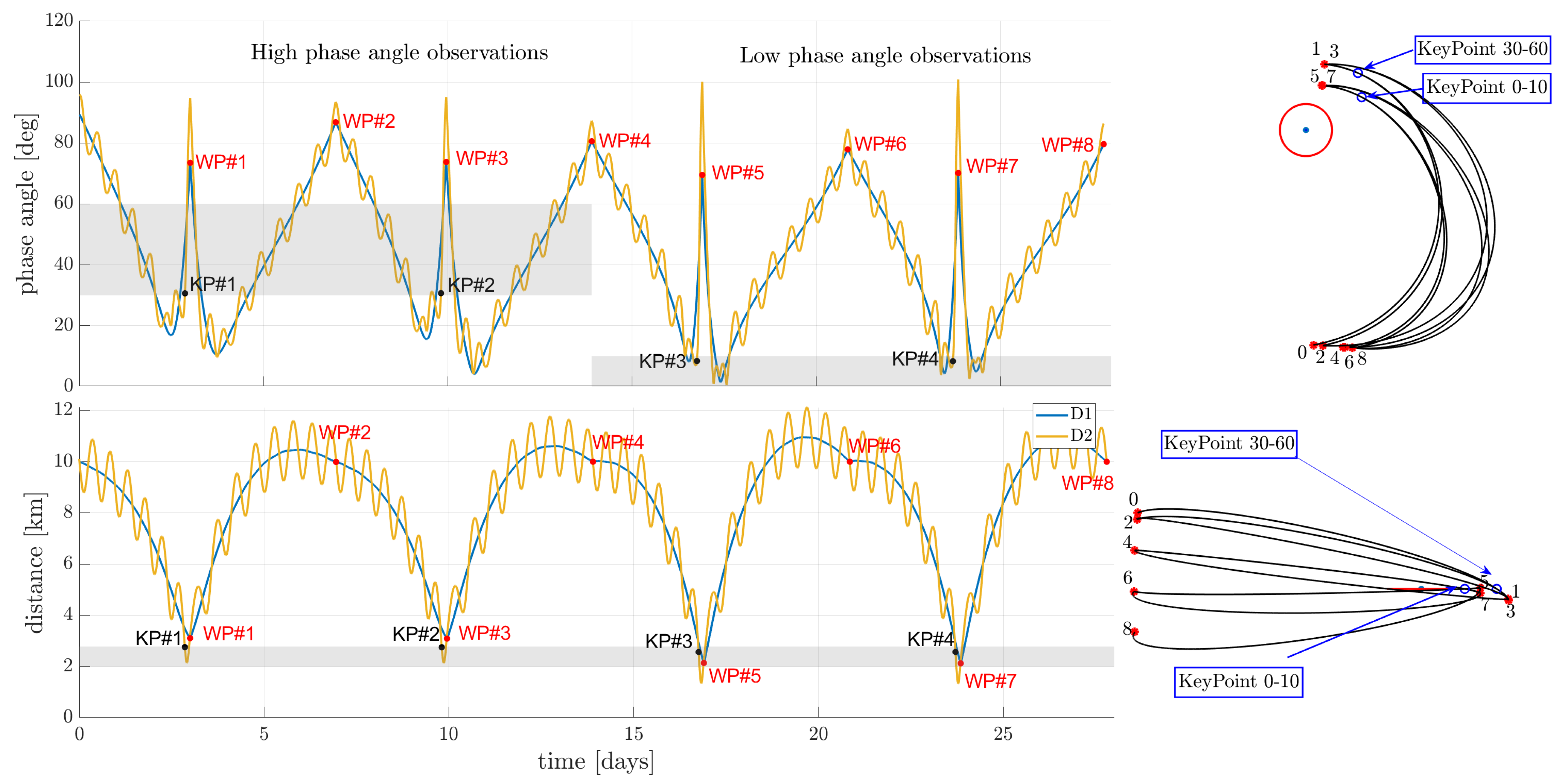
Option A is an eight-point loop built with a 3–4-day maneuvering pattern repeated four times.
Figure 2 shows the projection of the loop orbit on the
x–
y and
y–
z planes in the DidymosEquatorialSunSouth reference frame. The left plots of
Figure 2 show the time variation of the phase angles and distances with respect to D1 and D2. Red horizontal dashed lines delimit the science-admissible region for global mapping of D1 and D2, in terms of both the phase angle (between 5 and 25 deg) and the distance (between 2.780 and 4.572 km). A third dashed line is present in the bottom-right part of the figure representing the distance at which D1 saturates the NIR-FOV of ASPECT (1960 m). The time profiles show that the keypoint of each odd arc falls within the science-admissible region for imaging the crater, in terms of both the phase angle and distance.
3.3.2. CRP—Option B
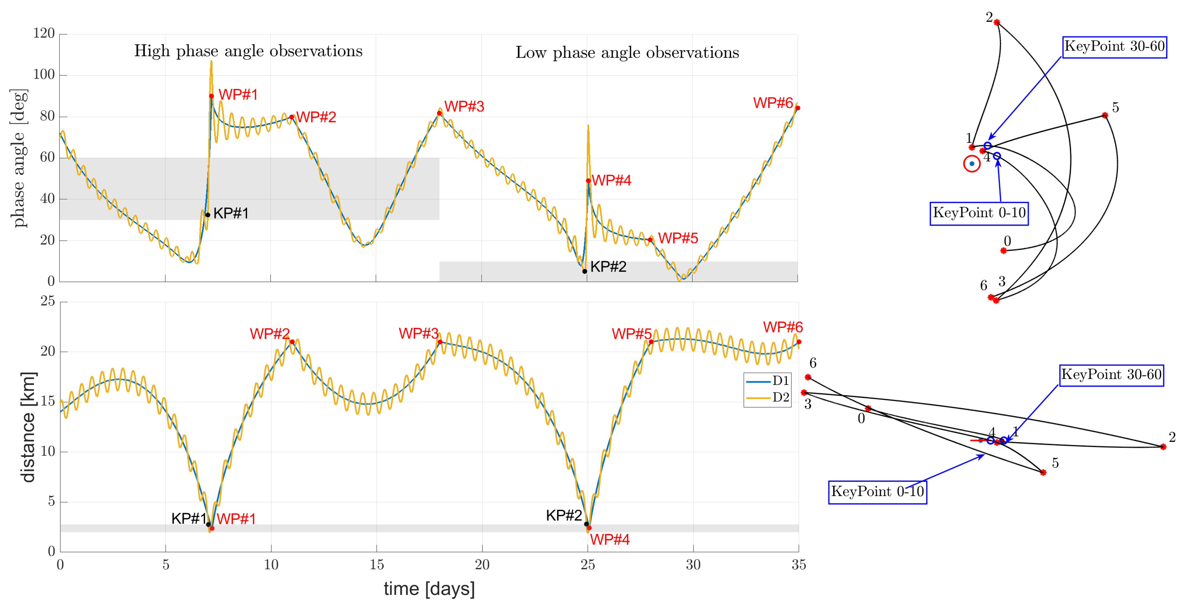
Option B is a six-point trajectory with a 7–4–7–7–3–7-day maneuvering pattern. The 7-day arcs can be seen as two arcs with a maneuvering frequency of 3 and 4 days, or vice versa, patched with a “zero-magnitude” maneuver in between. The Option B trajectory and geometry are shown in
Figure 3. The main differences between the two options are the number of passages through the keypoints, which is halved in Option B with respect to Option A, and the maneuvering frequency, which is lower in Option B. Maneuvering each week causes a reduction in the number of arcs (and so in the number of possible scientific observations) to keep the duration of the phase constant. On the other hand, maneuvers distant in time can be extremely beneficial from the operational point of view, as will be shown in
Section 4.
4. Trajectory Analysis
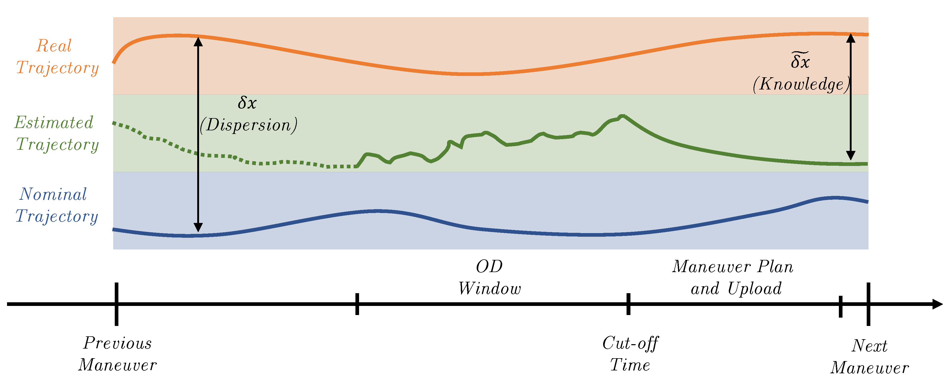
Applied trajectory design goes past the determination of the nominal trajectory. Once in space, the spacecraft will not follow the nominal trajectory due to the uncertainties affecting the dynamics, navigation and control, which are not considered in the nominal trajectory. Consequently, it is important to assess how much the real trajectory can differ from the nominal one and, in turn, to estimate the navigation costs, i.e., the stochastic cost associated with the correction maneuvers. This analysis measures the flyability of a trajectory, which is of great interest for practical applications. Indeed, when flying in highly non-linear environments the difference between nominal and real trajectories can be non-negligible, such that colliding with or escaping from the system can be a possibility. Thus, it is crucial to distinguish between nominal trajectories that exist only in the modeled reality and flyable orbits that are robust to uncertainties. The flyability of a trajectory can be assessed through two analyses: knowledge analysis and dispersion analysis.
4.1. Knowledge Analysis
The knowledge analysis (KA) assesses the achievable level of accuracy in the spacecraft-state knowledge. The term knowledge indicates the difference between the estimated trajectory, which can be inferred on the ground using indirect measurements on the state, and the real one. The level of accuracy of the state estimation is crucial since it is of interest in most of the mission operations. From the flight dynamics perspective, correction maneuvers are computed from the estimated deviation of the real trajectory with respect to the nominal one. Thus, the better the knowledge, the more effective the correction maneuvers. KA is based on the forward propagation of an initial knowledge represented as a Gaussian distribution centered in the nominal state
with a given initial covariance
. Uncertainties in the dynamics, such as residual accelerations, thruster inaccuracies or uncertainties in the dynamical model, usually produce an increase in the knowledge covariance in time. The covariance can decrease only through an orbit-determination process. During OD, pseudo-measurements are employed in a navigation filter to estimate the spacecraft state. The navigation of Milani is simulated considering radiometric measurements (range and range-rate between Hera and Milani) from the ISL and optical observations using landmark-based methods.
Table 4 shows all the information assumed to simulate Milani navigation. In the table, two sources of bias for the ISL measurements are considered: the typical instrument bias and the uncertainties in Hera’s state, which acts as a ground station. The NavCam uncertainties are expressed as a function of the nominal range
r. The noise is expressed as behavioral functions obtained after modeling a landmark-navigation technique. In this model, errors in the shape, asteroid orientation, scale factor, landmark detection and other perturbations have been considered and condensed into a simple equation.
The observables are processed with an extended Kalman filter (EKF) to estimate the state vector of the spacecraft. Biases are accounted for using Schimdt’s formulation [
20]. A dedicated analysis is performed for each mission phase. The filter is initialized considering the knowledge at the end of the previous phase, to which the additional uncertainty given by the maneuvers is added. Both the state deviation and the covariance matrix are then propagated with the associated dynamics up to the first measurement epoch, where the estimated trajectory is updated. The propagation is linear and is based on the nominal state transition matrix (STM), as performed in [
21]. Proceeding in this way, the state estimates are sequentially updated as new measurements are processed, leading to the position and velocity knowledge profiles. This is repeated up to the final epoch of the orbit-determination phase, obtaining the final spacecraft knowledge. To account for flight dynamics operations, a 48 h TAT has been considered, during which the following operations are performed:
- (i)
Data are sent from Milani to the ground through Hera.
- (ii)
Measurements are processed and an OD solution is produced.
- (iii)
Commands for the spacecraft are generated and validated on ground.
- (iv)
Data are sent back to Milani through Hera.
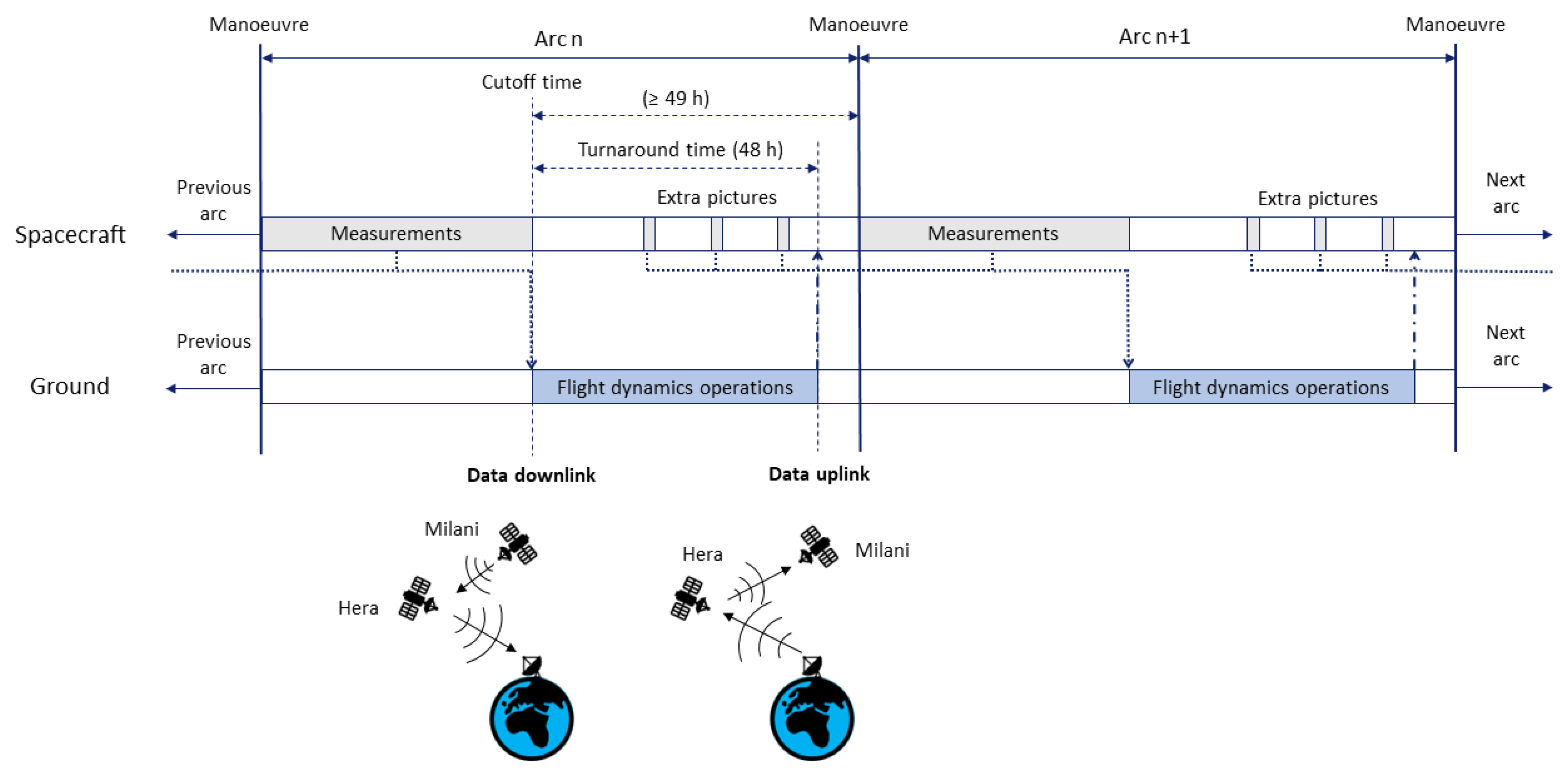
Furthermore, an additional margin of at least 1 h is considered between the data uplink and the execution of the maneuver. Therefore, the last observable that can be employed in the OD process is generated 49 h before the following maneuver. This represents the so-called cut-off time (COT). However, letting the spacecraft fly for 49 h without taking any measurements would increase the uncertainty unbearably in the next arc, so the envisaged strategy is to take navigation images during the COT also. These images are then used on the ground together with data taken during the following arc in order to improve the post-maneuver knowledge by considering the observables of the spacecraft state before the maneuver itself. Therefore, for each arc two covariances are propagated: one represents the actual ground knowledge for the current arc and considers only the measurement available before the COT, while the other represents the knowledge that will be obtained after processing the images taken during the COT and used for the following arc.
The strategy is illustrated in
Figure 4.
The following assumptions are considered throughout the analysis:
Navigation is considered to be relative to the Didymos system’s barycentre.
A maneuvering error is considered with the uncertainty shown in
Table 5.
Range and range-rate measurements are supposed to be always available.
SRP and residual acceleration are modeled as Gauss–Markov (GM) [
21] processes, with the properties shown in
Table 5.
Uncertainty on the gravitational attraction is treated as a consider parameter. The assumed 1-sigma uncertainty at the beginning of the mission is of 3.5% of the nominal gravitational attraction of the system (35 m3 s−2). This value was taken from the NASA Horizon’s Didymos reference model of July 2022, properly reduced considering the contribution that DART and Hera will give for the gravity field estimation before Milani’s release. CRP takes places a month after the release, when our analyses show that the uncertainty over the gravitational parameter is reduced to 10−4 m3 s−2. This uncertainty is considered relevant only on D1, to which it is applied in the analysis.
ISL measurement starts 6 h after the beginning of the arc and ends 3 h before the cut-off time. The range measures are taken every 3 h, and the range-rate every 1 h.
The optical measurement plan depends on the strategy, due to the different number of arcs and the duration of each one (
Section 3.3).
- –
For CRP-Option A: Seven optical measurements are taken in a single arc, four of them before the cut-off time for the OD of the current arc, the other three after the cut-off time, and they will be used for the OD of the next arc.
- –
For CRP-Option B: 12 optical measurements are taken in a single arc, seven of them before the cut-off time for the OD of the current arc, the other five after the cut-off time, and they will be used for the OD of the next arc.
Please note that the number of pictures that can be taken for navigation purposes is bounded by the limited data budget available.
4.2. Dispersion Analysis
The dispersion analysis (DA) shows the statistics of the real trajectory. Indeed, the term dispersion indicates the stochastic distance between the real and the nominal trajectory. DA can be performed with a Monte Carlo analysis, which accounts for the source of uncertainty in the spacecraft dynamics. For each run, the initial nominal state
is perturbed with an initial uncertainty represented as a Gaussian distribution centered in the nominal state with a given initial covariance
. This initial perturbed state is propagated under the effect of the perturbed dynamic up to the COT, when the observables are downlinked. Here, the estimated state is simulated by perturbing the true CubeSat state with a Gaussian uncertainty whose covariance is given by the KA. The estimated state is then propagated up to the correction time and the correction maneuver is computed according to it. At the same time, the real trajectory is propagated up to the correction time and the corresponding maneuver is applied before proceeding with the next leg. Usually, for deep-space operations a correction maneuver is scheduled each week. For CPOs, a correction is usually needed at the earliest convenience. For Milani, correction maneuvers are usually executed together with the nominal maneuvers because of the limitations imposed by the flight dynamics operations. As the OD improves knowledge, correction maneuvers reduce the dispersion. In order to compute them a guidance flow is needed.
Figure 5 shows the approach followed.
In Milani, the differential guidance, a commonly used guidance strategy for interplanetary missions [
22], is applied. In this formulation, the whole trajectory is subdivided into different legs. At the extremal points of a single leg, two maneuvers are applied to cancel both the position and the velocity deviations on the final leg point. However, the final impulse is usually not applied in practice, since at the time of arrival at the final point a new maneuver is calculated. Based on this, the maneuver can be computed by minimizing the deviations from the nominal state at the final point in a least-square residual sense. Thus, the maneuver that must be applied at the time
in order to cancel out the deviations at time
is computed as:
where
and
are the estimated position and velocity deviation;
,
,
and
are the three-by-three blocks of the STM
from time
to time
associated with the nominal trajectory; and
q is a factor used only to adjust the dimensions. When control impulses are foreseen at the nominal maneuvering points, the correction maneuvers are superimposed on the nominal ones. This procedure is repeated up to the final time. The estimation of the total navigation cost is obtained as the sum of all the maneuvers. The assumptions made during the DA are summarized and listed below:
Each arc is initialized considering the dispersion at the end of the previous phase, to which the additional uncertainty given by the maneuvers is added.
A thrust misalignment of 5% in magnitude and 2 deg in angle (3-sigma) is considered.
SRP and residual acceleration are modeled as Gauss–Markov process with the same properties shown in
Table 5.
The uncertainty in the gravitational attraction is considered with the properties shown in
Table 5.
4.3. Results
The knowledge and dispersion analysis results for both the CRP options are shown in this section.
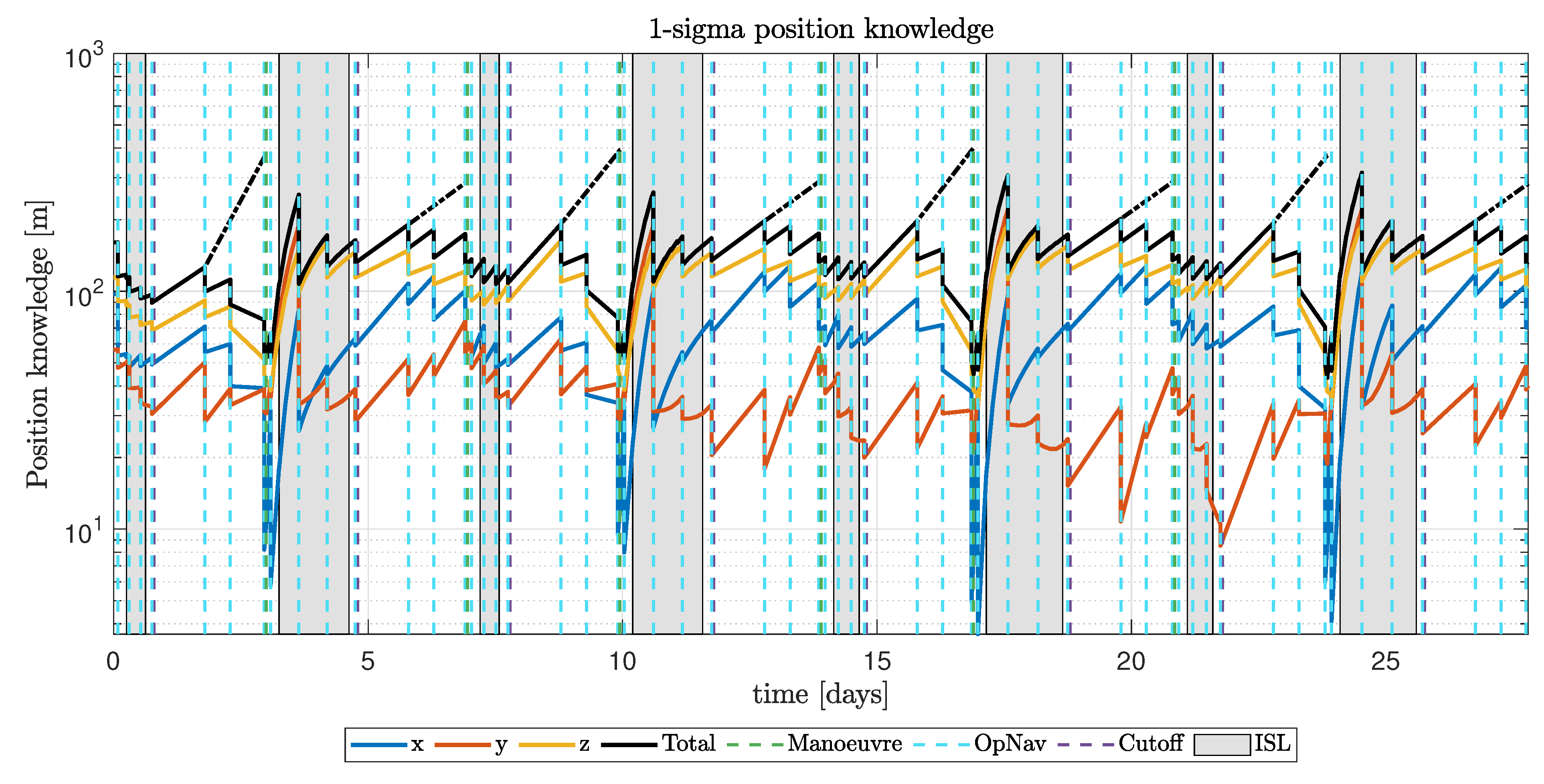
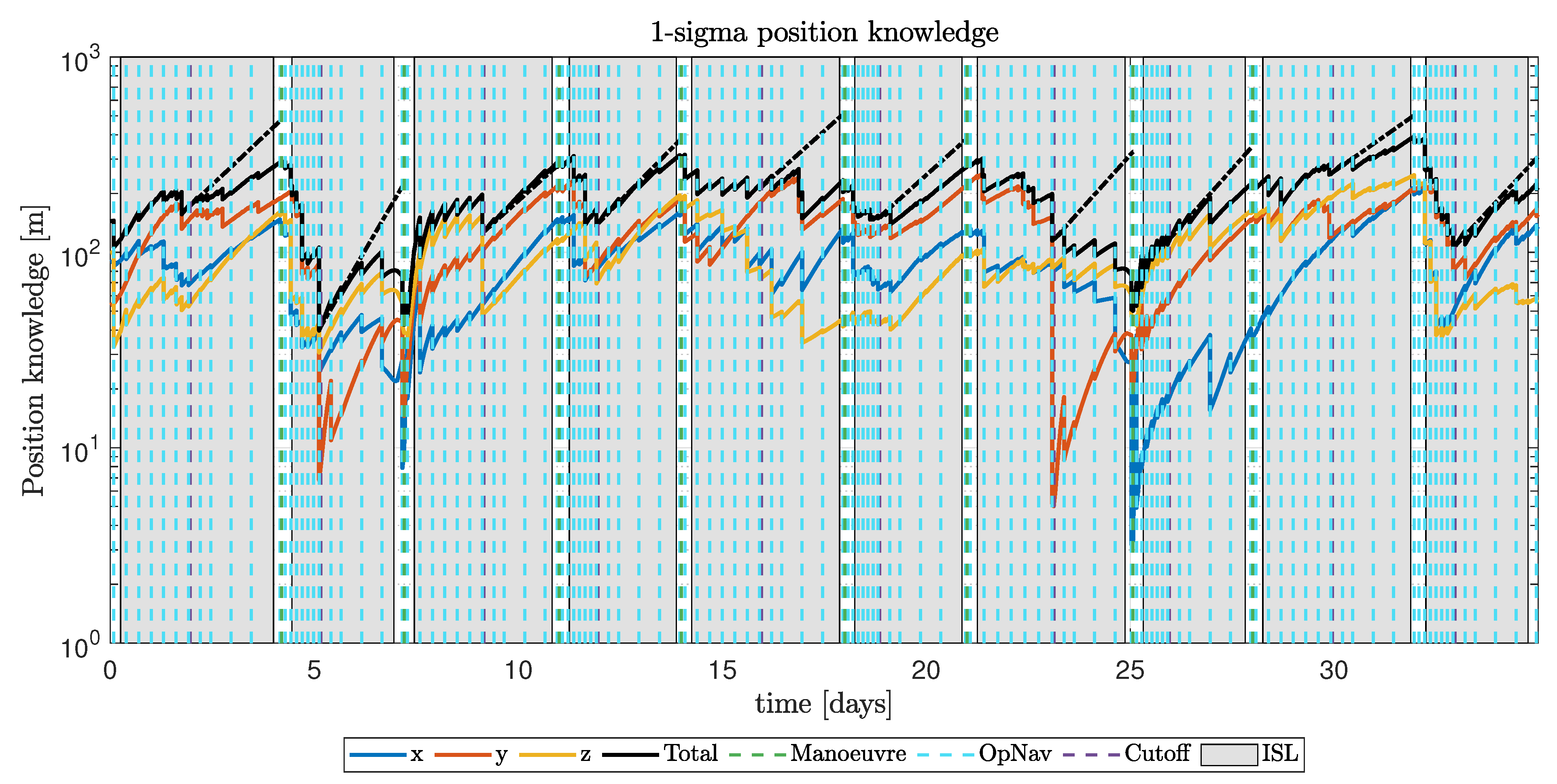
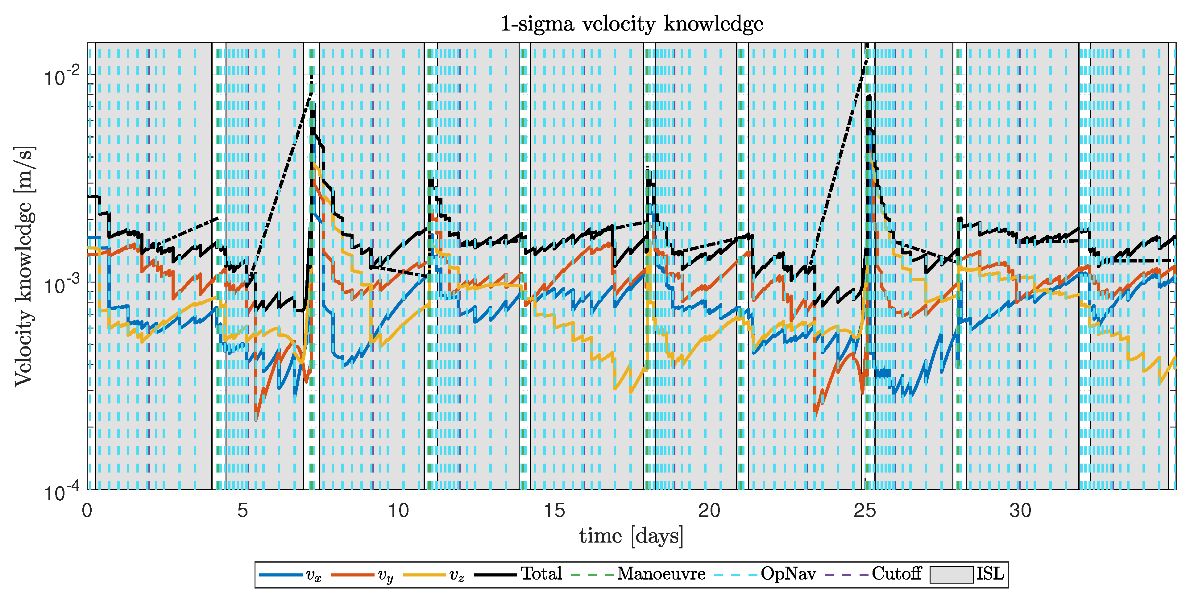
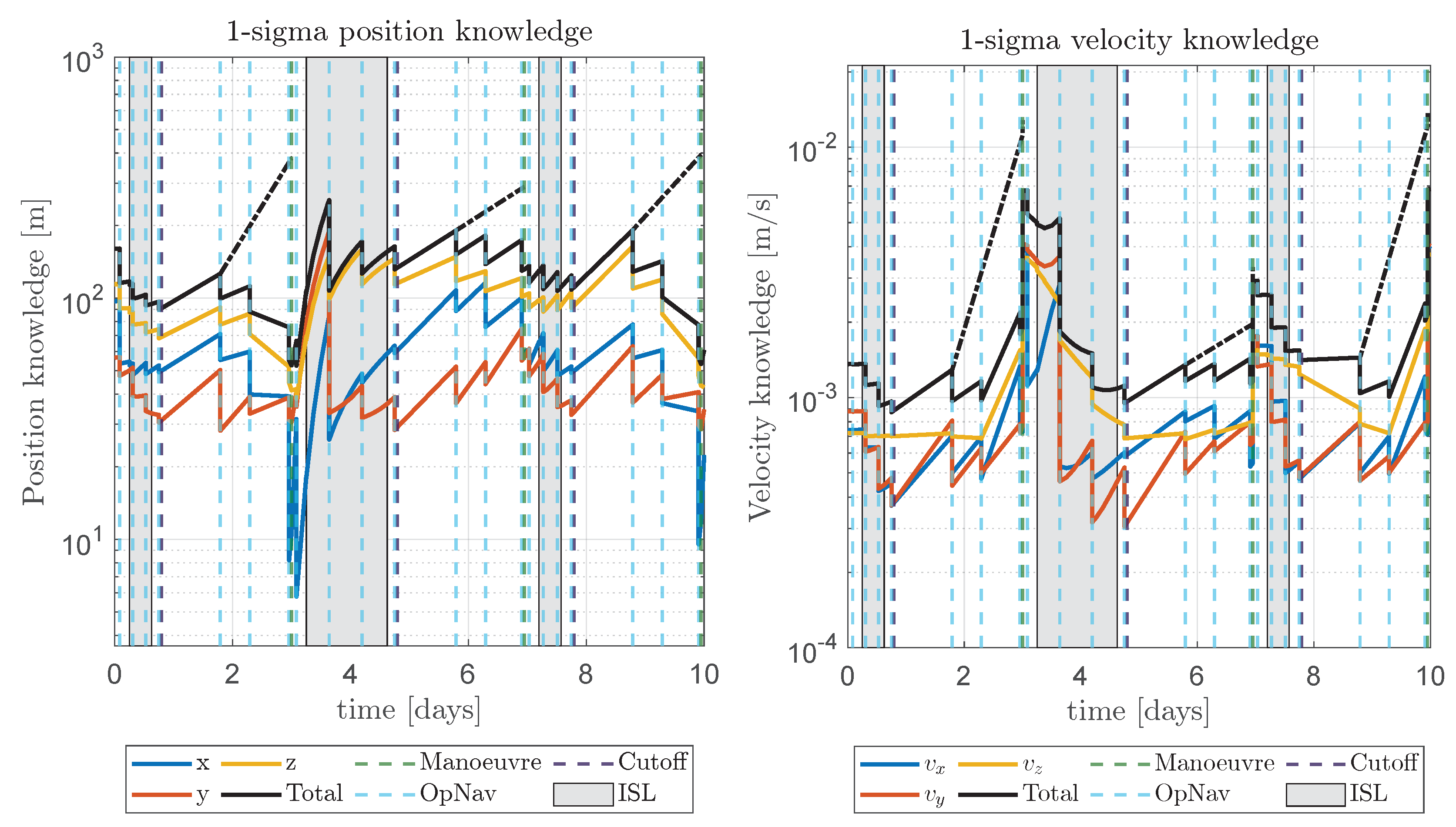
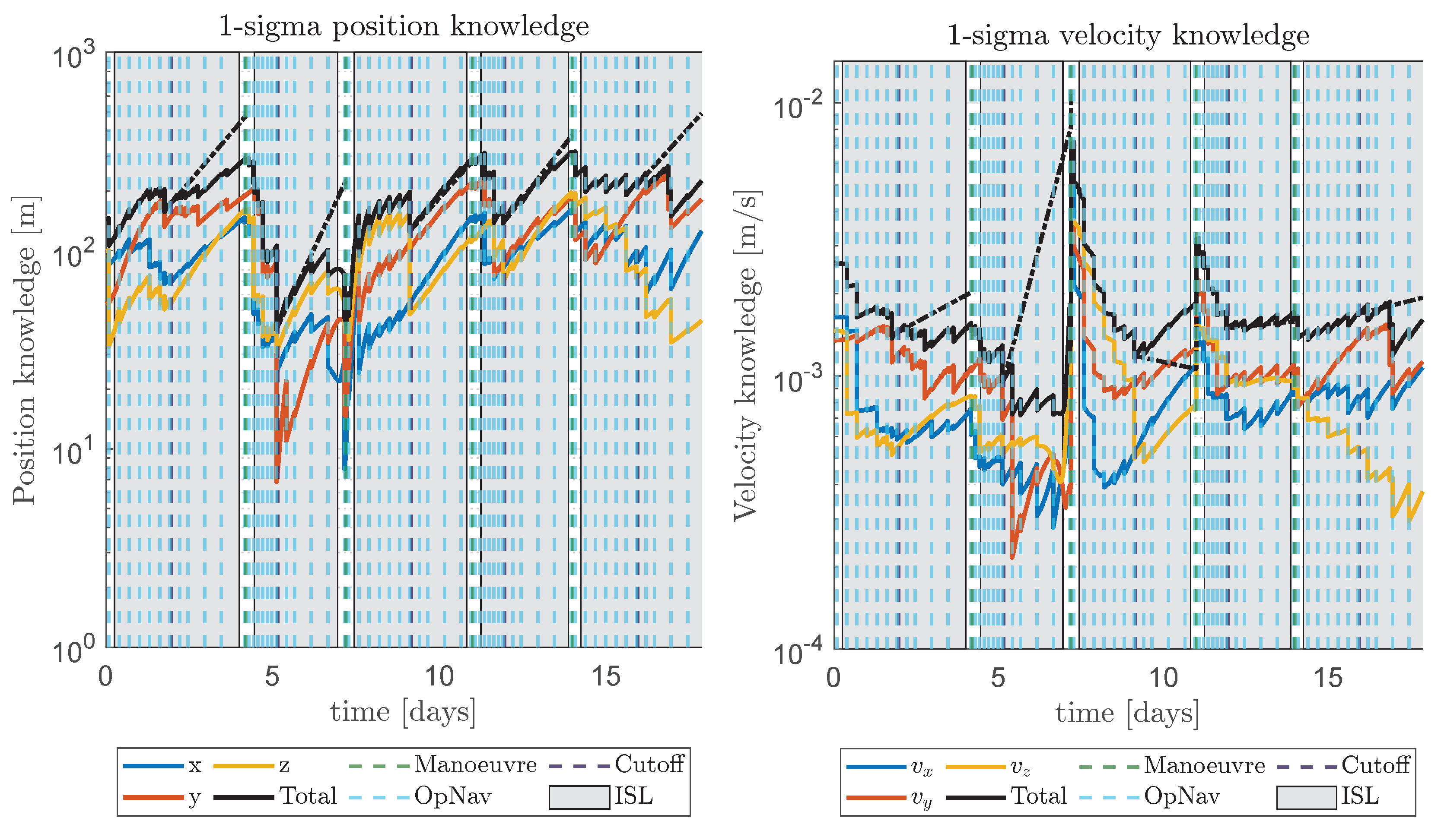
Figure 6 and
Figure 7 show the position knowledge for Option A and Option B, respectively, while
Figure 8 and
Figure 9 show the velocity knowledge. For a better comparison, a zoom in the first days of the CRP is given in
Figure 10 and
Figure 11. The total knowledge is computed as the square root of the covariance trace. For both options, the knowledge computed on-ground at the maneuver instants is on the order of a few hundreds of meters for the position and less than 1 cm/s for the velocity. No particular differences can be highlighted between the two options. Contrarily, the two solutions differ significantly from the dispersion point of view, as shown in
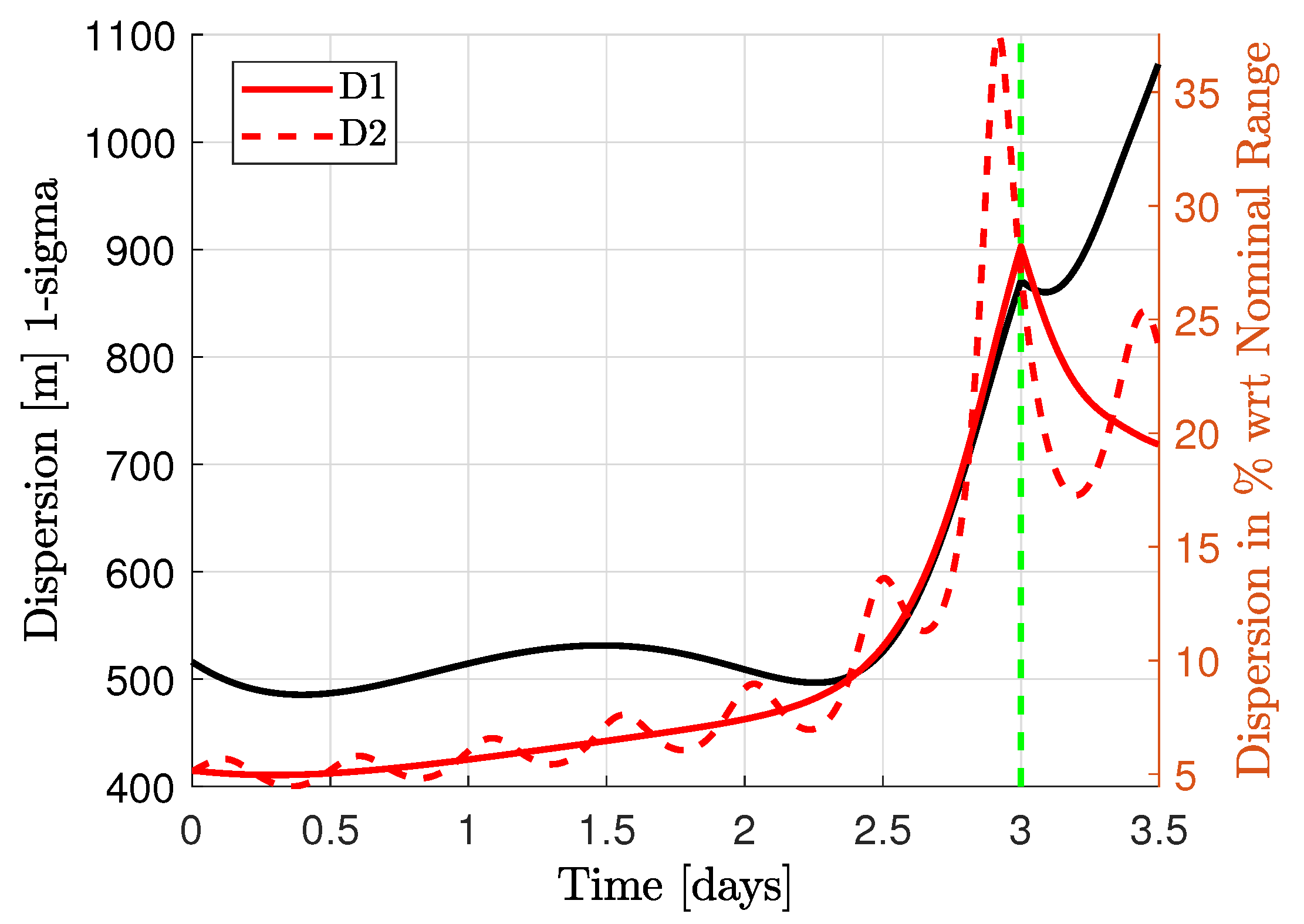
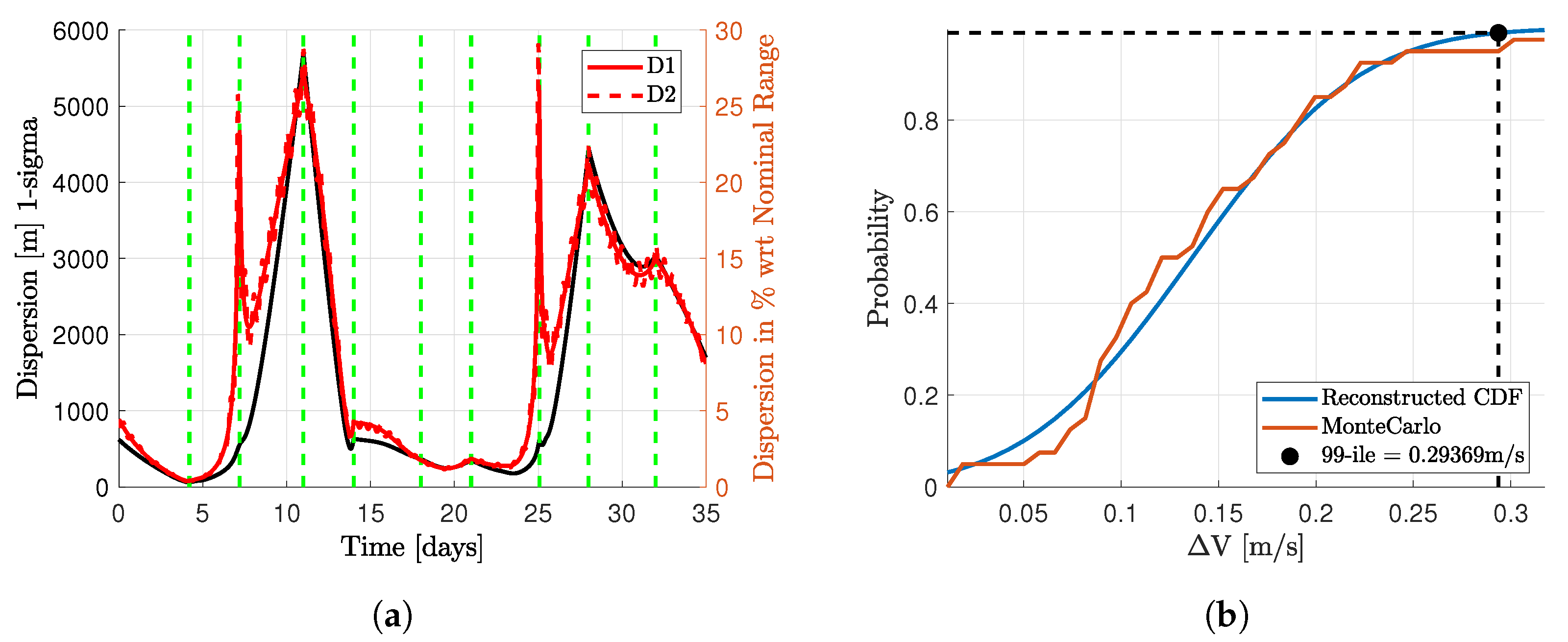
Figure 12 and
Figure 13, even if they have the same initial point and initial distribution. The figures show both the absolute dispersion (black) and relative dispersion with respect to the nominal distance between the spacecraft and the asteroids (red).
Figure 12 clearly shows the unflyability of Option A. The error introduced by the maneuver is so high that the CubeSat reaches a relative dispersion of 33% (1-sigma) before any possibility of executing a correction maneuver. A relative dispersion of 33% (1-sigma) means that there is a non-negligible collision probability with the asteroid. Indeed, in this condition there can be trajectories that impact the asteroid surface inside the 3-sigma probability region. A correction maneuver is then needed somewhere before approaching the system to reduce the relative dispersion. Considering the operational constraints on the maneuvering frequency, the only possibility of uploading a correction maneuver before approaching the system is to increase the arc duration up to 7 days. In this way, a cleanup maneuver targeting the waypoint close to the system can be scheduled in the middle of the arc where no concurrent expensive maneuvers are scheduled. The navigation costs for this option are not shown since the trajectory is not flyable.
Figure 13 shows that the dispersion for CRP Option B is still high, but it can be considered reliable in terms of collision risks. For this reason, the dispersion analysis results for the entire mission phase are presented. Furthermore, the cumulative distribution function (CDF) of the navigation cost for this option is also reported. The results are satisfying since the 99th percentile of the CDF corresponds roughly to 5% of the total mission cost.
5. Conclusions
In this work, the approach to the mission analysis pipeline for a CubeSat in close-proximity operations is presented. The case study is Milani, a CubeSat mission around a binary asteroid. Two design options have been presented for the close-range phase of the mission. Option A was the first solution considered. The trajectory appeared to be simple and all the requirements and constraints were considered. However, even if a nominal solution exists, the navigation assessment revealed that the trajectory is not flyable due to a non-negligible impact risk. The introduction of cleanup maneuvers in the middle of the arc appears to be fundamental to reduce the dispersion before approaching the system. Consequently, Option B was designed to be as robust as possible to the uncertainties affecting Option A the most while accounting for operational constraints.
The Milani mission analysis shows how operational constraints and uncertainties can be relevant to designing flyable trajectories for CubeSats. Operating in strongly perturbed environments, such as around small bodies, with CubeSats shows the importance of including in the preliminary analyses not only on-ground operations considerations in the design process, but also trajectory-navigation assessment in order to avoid unflyable solutions. While it is true that these assessment are generally performed, for traditional spacecraft missions they are commonly performed after the design. This work has shown how trajectory design should include such analyses in the design process due to CubeSats being more prone to uncertainties. In fact, the Milani dispersion analysis shows how the existing nominal orbits can be completely unflyable when considering the uncertainties in the maneuver execution or in the dynamical model considered.
Author Contributions
Conceptualization, C.B., F.P., C.G., F.F. and F.T.; methodology, C.B., F.P., C.G., F.F. and F.T.; software, C.B., F.P. and C.G.; validation, C.B. and F.P.; formal analysis, C.B.; investigation, C.B.; resources, F.F. and F.T.; data curation, C.B., F.P., C.G., F.F. and F.T.; writing—original draft preparation, C.B.; writing—review and editing, F.P., C.G., F.F. and F.T.; visualization, C.B. and F.P.; supervision, F.F. and F.T.; project administration, F.T.; funding acquisition, F.F. and F.T. All authors have read and agreed to the published version of the manuscript.
Funding
The work has received funding under a Tyvak International contract within ESA Contract No. 1222343567/62/NL/GLC.
Data Availability Statement
Trajectories generated in this work can be found in the Hera SPICE Kernel Dataset managed by ESA as SPICE kernels. Other data presented in this study are available on request from the corresponding author.
Acknowledgments
Part of the work presented in this paper has been performed under a Tyvak International contract within ESA Contract No. 1222343567/62/NL/GLC. The authors would like to acknowledge the support received by the whole Milani Consortium.
Conflicts of Interest
The authors declare no conflict of interest.
References
- Veverka, J.; Farquhar, B.; Robinson, M.; Thomas, P.; Murchie, S.; Harch, A.; Antreasian, P.G.; Chesley, S.R.; Miller, J.K.; Owen, W.M.; et al. The landing of the NEAR-Shoemaker spacecraft on asteroid 433 Eros. Nature 2001, 413, 390–393. [Google Scholar] [CrossRef] [PubMed]
- Furfaro, R.; Cersosimo, D.; Wibben, D.R. Asteroid Precision Landing via Multiple Sliding Surfaces Guidance Techniques. J. Guid. Control Dyn. 2013, 36, 1075–1092. [Google Scholar] [CrossRef]
- Yoshikawa, K.; Sawada, H.; Kikuchi, S.; Ogawa, N.; Mimasu, Y.; Ono, G.; Takei, Y.; Terui, F.; Saiki, T.; Yasuda, S.; et al. Modeling and analysis of Hayabusa2 touchdown. Astrodynamics 2020, 4, 119–135. [Google Scholar] [CrossRef]
- Accomazzo, A.; Ferri, P.; Lodiot, S.; Pellon-Bailon, J.L.; Hubault, A.; Porta, R.; Urbanek, J.; Kay, R.; Eiblmaier, M.; Francisco, T. Rosetta operations at the comet. Acta Astronaut. 2015, 115, 434–441. [Google Scholar] [CrossRef]
- Walker, R.; Binns, D.; Bramanti, C.; Casasco, M.; Concari, P.; Izzo, D.; Feili, D.; Fernandez, P.; Fernandez, J.G.; Hager, P.; et al. Deep-space CubeSats: Thinking inside the box. Astron. Geophys. 2018, 59, 24–30. [Google Scholar] [CrossRef]
- Martin-Mur, T.J.; Young, B. Navigating MarCO, the First Interplanetary CubeSats. In Proceedings of the 18th Australian International Aerospace Congress, Melbourne, Australia, 24–28 February 2019. [Google Scholar]
- Topputo, F.; Wang, Y.; Giordano, C.; Franzese, V.; Goldberg, H.; Perez-Lissi, F.; Walker, R. Envelop of reachable asteroids by M-ARGO CubeSat. Adv. Space Res. 2021, 67, 4193–4221. [Google Scholar] [CrossRef]
- McNutt, L.; Johnson, L.; Kahn, P.; Castillo-Rogez, J.; Frick, A. Near-Earth asteroid (NEA) scout. In Proceedings of the AIAA Space 2014 Conference and Exposition, San Diego, CA, USA, 4–7 August 2014. [Google Scholar]
- Bottiglieri, C.; Piccolo, F.; Rizza, A.; Giordano, C.; Pugliatti, M.; Franzese, V.; Ferrari, F.; Topputo, F. Trajectory design and orbit determination for Hera’s Milani CubeSat. In Proceedings of the 2021 AAS/AIAA Astrodynamics Specialist Conference, Virtual, 9–11 August 2021. [Google Scholar]
- Karatekin, O.; Goldberg, H.; Prioroc, C.L.; Villa, V. Juventas: Exploration of a binary asteroid system with a CubeSat. In Proceedings of the International Astronautical Congress, IAC, Washington, DC, USA, 21–25 October 2019. [Google Scholar]
- Ferrari, F.; Franzese, V.; Pugliatti, M.; Giordano, C.; Topputo, F. Trajectory Options for Hera’s Milani CubeSat Around (65803) Didymos. J. Astronaut. Sci. 2021, 68, 973–994. [Google Scholar] [CrossRef]
- Cheng, A.; Atchison, J.; Kantsiper, B.; Rivkin, A.; Stickle, A.; Reed, C.; Galvez, A.; Carnelli, I.; Michel, P.; Ulamec, S. Asteroid Impact and Deflection Assessment mission. Acta Astronaut. 2015, 115, 262–269. [Google Scholar] [CrossRef]
- Sarli, B.V.; Atchison, J.A.; Ozimek, M.T.; Englander, J.A.; Barbee, B.W. Double Asteroid Redirection Test Mission: Heliocentric Phase Trajectory Analysis. J. Spacecr. Rocket. 2019, 56, 546–558. [Google Scholar] [CrossRef]
- Bottiglieri, C.; Piccolo, F.; Rizza, A.; Pugliatti, M.; Franzese, V.; Giordano, C.; Ferrari, F.; Topputo, F. Mission Analysis and Navigation Assessment for Hera’s Milani CubeSat. In Proceedings of the 4S Symposium, Vilamoura, Portugal, 16–20 May 2022. [Google Scholar]
- Chobotov, V.A. Orbital Mechanics; AIAA Education Series; American Institute of Aeronautics and Astronautics: Washington, DC, USA, 1991. [Google Scholar]
- Pugliatti, M.; Piccolo, F.; Rizza, A.; Franzese, V.; Topputo, F. The vision-based guidance, navigation, and control system of Hera’s Milani Cubesat. Acta Astronaut. 2023. [Google Scholar] [CrossRef]
- Palomba, E.; Longobardo, A.; Dirri, F.; Zampetti, E.; Biondi, D.; Saggin, B.; Bearzotti, A.; Macagnano, A. VISTA: A μ-Thermogravimeter for Investigation of Volatile Compounds in Planetary Environments. Orig. Life Evol. Biosph. 2016, 46, 273–281. [Google Scholar] [CrossRef] [PubMed]
- Kohout, T.; Näsilä, A.; Tikka, T.; Granvik, M.; Kestilä, A.; Penttilä, A.; Kuhno, J.; Muinonen, K.; Viherkanto, K.; Kallio, E. Feasibility of asteroid exploration using CubeSats—ASPECT case study. Adv. Space Res. 2018, 62, 2239–2244. [Google Scholar] [CrossRef]
- Ferrari, F.; Franzese, V.; Pugliatti, M.; Giordano, C.; Topputo, F. Preliminary mission profile of Hera’s Milani CubeSat. Adv. Space Res. 2021, 67, 2010–2029. [Google Scholar] [CrossRef]
- Simon, D. Optimal State Estimation: Kalman, H Infinity, and Nonlinear Approaches; John Wiley & Sons: Hoboken, NJ, USA, 2006. [Google Scholar]
- Tapley, B.D.; Schutz, B.E.; Born, G.H. Statistical Orbit Determination; Elsevier: Amsterdam, The Netherlands, 2004. [Google Scholar] [CrossRef]
- Dei Tos, D.A.; Rasotto, M.; Renk, F.; Topputo, F. LISA Pathfinder mission extension: A feasibility analysis. Adv. Space Res. 2019, 63, 3863–3883. [Google Scholar] [CrossRef]
Figure 1.
Schematic for the “keypoint” choice. The keypoint is placed where the crater can be observed respecting all the scientific requirements, i.e., within required distances (dashed annulus) and phase angle (dashed cone). The maneuver points of the observation arcs are chosen to avoid going into the night side.
Figure 2.
CRP—Option A orbit strategy. Keypoints are depicted as black dots, waypoints as red dots. Grey areas show distance requirements for the crater observations. In the figure on the left, numbers indicate the waypoints.
Figure 2.
CRP—Option A orbit strategy. Keypoints are depicted as black dots, waypoints as red dots. Grey areas show distance requirements for the crater observations. In the figure on the left, numbers indicate the waypoints.
Figure 3.
CRP—Option B orbit strategy. Keypoints are depicted as black dots, waypoints as red dots. Grey areas show distance requirements for the crater observations.In the figure on the left, numbers indicate the waypoints.
Figure 3.
CRP—Option B orbit strategy. Keypoints are depicted as black dots, waypoints as red dots. Grey areas show distance requirements for the crater observations.In the figure on the left, numbers indicate the waypoints.
Figure 4.
Milani knowledge analysis timeline illustration.
Figure 4.
Milani knowledge analysis timeline illustration.
Figure 5.
Dispersion analysis approach.
Figure 5.
Dispersion analysis approach.
Figure 6.
1-sigma position knowledge during CRP Option A. The dashed black line is the knowledge obtained considering only observables generated before COT.
Figure 6.
1-sigma position knowledge during CRP Option A. The dashed black line is the knowledge obtained considering only observables generated before COT.
Figure 7.
1-sigma position knowledge during the CRP Option B. The dashed black line is the knowledge obtained considering only observables generated before COT.
Figure 7.
1-sigma position knowledge during the CRP Option B. The dashed black line is the knowledge obtained considering only observables generated before COT.
Figure 8.
1-sigma velocity knowledge during CRP Option A. The dashed black line is the knowledge obtained considering only observables generated before COT.
Figure 8.
1-sigma velocity knowledge during CRP Option A. The dashed black line is the knowledge obtained considering only observables generated before COT.
Figure 9.
1-sigma velocity knowledge during CRP Option B. The dashed black line is the knowledge obtained considering only observables generated before COT.
Figure 9.
1-sigma velocity knowledge during CRP Option B. The dashed black line is the knowledge obtained considering only observables generated before COT.
Figure 10.
1-sigma knowledge during the first 10 days of CRP Option A.
Figure 10.
1-sigma knowledge during the first 10 days of CRP Option A.
Figure 11.
1-sigma knowledge during the first 17 days of CRP Option B.
Figure 11.
1-sigma knowledge during the first 17 days of CRP Option B.
Figure 12.
Dispersion analysis results for CRP Option A. Maneuvers are shown as dashed green lines. The graph stops after the first maneuver since a non-negligible collision risk is reached. Manoeuvres are dashed green lines.
Figure 12.
Dispersion analysis results for CRP Option A. Maneuvers are shown as dashed green lines. The graph stops after the first maneuver since a non-negligible collision risk is reached. Manoeuvres are dashed green lines.
Figure 13.
Dispersion analysis results for CRP Option B. (a) Dispersion during CRP Option B. Manoeuvres are dashed green lines. (b) Cumulative distribution function of the navigation costs. Dot shows the 99th percentile.
Figure 13.
Dispersion analysis results for CRP Option B. (a) Dispersion during CRP Option B. Manoeuvres are dashed green lines. (b) Cumulative distribution function of the navigation costs. Dot shows the 99th percentile.
Table 1.
Dynamical parameters.
Table 1.
Dynamical parameters.
| Parameter | Symbol | Value |
|---|
| D1 gravitational parameter | | 34.901 m3/s2 |
| D2 gravitational parameter | | 0.3246 m3/s2 |
| Sun gravitational parameter | | m3/s2 |
| Solar flux | | 1367 W/m2 |
| Speed of light | c | m/s |
| Astronomical unit | | m |
| Reflectivity coefficient | | 1.25 |
| Surface area | A | 0.51 m2 |
| Spacecraft mass | M | 12 kg |
Table 2.
Summary of the observation windows requirements during CRP.
Table 2.
Summary of the observation windows requirements during CRP.
| Feature | Resolution [m/px] | Distance [m] | Phase Angle [deg] |
|---|
| D2 global coverage | 1 | 5480 | [0–60] |
| Crater on D2 | 0.5 | 2780 | [0–10] |
| [0–60] |
Table 3.
Milani trajectory-design constraints.
Table 3.
Milani trajectory-design constraints.
| Constraint | Description |
|---|
| Phase-angle operation range | To enable optical navigation and science, the phase angle relative to both D1 and D2 should always be below 90 deg |
| Turn-around time | The minimum time between the downlink of the information and the uplink of the instructions is 48 h |
| Communication window | Milani can communicate with the ground only within the Hera communication windows |
| Maneuvering frequency | Maneuvers should be scheduled with a 3–4–3–4-day pattern together with Hera |
Table 4.
Relevant assumed instrument parameters.
Table 4.
Relevant assumed instrument parameters.
| Instrument | Noise on the Measurement [1-Sigma] | Bias |
|---|
| NavCam | (range) | 2 m (range) |
| (angle) | 32.4 arcsec (angle) |
| ISL (Range) | 0.5 m | 150 m |
| ISL (Range-Rate) | 1.5 cm s−1 | 3 cm s−1 |
Table 5.
Uncertainties in the dynamics.
Table 5.
Uncertainties in the dynamics.
| Uncertainty | Value [1-Sigma] |
|---|
| Gravity uncertainty | 10−4 m3 s−2 |
| Thruster | 1.67% (magnitude), 0.67 deg (direction) |
| SRP | 8% (magnitude), 1 day (correlation time) |
| Residual acceleration | 5 × 10⁻⁹ m s−2, 1 day (correlation time) |
| Disclaimer/Publisher’s Note: The statements, opinions and data contained in all publications are solely those of the individual author(s) and contributor(s) and not of MDPI and/or the editor(s). MDPI and/or the editor(s) disclaim responsibility for any injury to people or property resulting from any ideas, methods, instructions or products referred to in the content. |
© 2023 by the authors. Licensee MDPI, Basel, Switzerland. This article is an open access article distributed under the terms and conditions of the Creative Commons Attribution (CC BY) license (https://creativecommons.org/licenses/by/4.0/).


