Feasibility Analysis of Autonomous Orbit Determination and Gravity-Field Recovery around Asteroids Using Inter-Satellite Range Data

Abstract

Autonomous navigation and orbit determination are key problems of asteroid exploration missions. Inter-satellite range link is a type of measurement widely used in the orbit determination of Earth satellites, but not so widely used in missions around small bodies. In our study, we assume that highly accurate inter-satellite range data can be obtained around small bodies between the chief spacecraft and some low-cost deputies, and study the feasibility of simultaneous autonomous orbit determination of the spacecraft and the gravity-field recovery without the support from ground stations. After the feasibility analysis, two modified methods are proposed. Both methods demonstrate obvious improvements in both the convergence region and the accuracy. One remark is that the inter-satellite range data can be also used together with various observation data from ground stations to enhance the accuracy of the determined orbits and the gravity field.

1. Introduction

Nowadays, small bodies are interesting targets of in-suite explorations. Up to now, many missions have visited these objects. Determining the spacecraft’s orbit and the asteroid’s gravity field is one of the goals for these missions. To this end, the current technology heavily depends on observations from ground stations. There are several types of observation data often used in asteroid missions. In the earliest missions, Doppler and range-measurement are main types of data used in missions, such as the NEAR-Shoemaker and the DAWN mission [1,2,3]. VLBI data is also widely used. For example, during the Chang’e-2 flyby of the asteroid Toutatis, its orbit was determined by the VLBI data together with the USB (Unified S-Band) data [4]. Delta Differential One-way Ranging (DDOR) is a highly accurate measurement based on the VLBI technology [5] and was used in the OSIRIS-Rex mission [6,7].

Most asteroids are irregularly shaped. Many studies have been carried out on asteroid shapes and gravity-field models. For example, the polyhedron model is one of the most widely used asteroid shape models [8], but its associated form of gravity field is inconvenient to use in the gravity field recovery from observations. For elongated asteroids, a simple rotating mass dipole model is used to rapidly model the gravity field [9]. Despite of these gravity models, the most commonly used one in the asteroid’s gravity field recovery is still the well-known spherical harmonics. By recovering the gravity harmonic coefficients, density and internal structures of an asteroid can be inferred [10,11,12]. The gravity coefficients are usually measured simultaneously with the spacecraft’s orbit. For the first asteroid exploration mission, NEAR-Shoemaker, the gravity field up to the fourth order and degree was determined [1]. Using Doppler and range data of the Dawn spacecraft, Park and Konopliv et al. obtained a gravity field up to 20th order and degree for Vesta and 18th order and degree for Ceres, the two most massive asteroids in the asteroid belt [2,3,10,13]. For asteroids of hundreds of meters in diameter or even smaller, it is usually difficult to obtain a high order and degree gravity field using traditional methods. One exception is the asteroid Bennu which is only about 450 m in diameter. In the OSIRIS-Rex mission, angle-measurement data between the spacecraft and particles around the asteroid made it possible to determine the gravity field to a high precision of 10th order and degree [14,15].

Experience from the OSIRIS-Rex mission indicates that accurate relative measurement around the asteroid may help improve the accuracy of the gravity-field recovery. We do not always have the chance to obtain relative angle measurement data as we did in the OSIRIS-Rex mission because not all targets have particles ejected from their surface, but we can use artificial relative-measurement data such as the inter-satellite range measurement, which is already extensively used in many applications around the Earth. For example, in the global navigation satellite system (GNSS), the addition of inter-satellite range data to the ground-observation data can significantly improve the accuracy of orbit determination [16,17,18]. In addition, in the GRACE-FO mission, the precise inter-satellite range data are used to obtain the high-order gravity field of the Earth [19].

An intuitive idea is to borrow this technology for asteroid missions. That is to say, we build accurate inter-satellite links between the spacecraft formation with one chief spacecraft and some cheap deputies which can move closer to the asteroid’s surface. For spacecraft formations in the proximity of asteroids, autonomous navigation using multiple sensors was already studied [20]. For Earth satellites, it is impossible to autonomously determine the satellites’ orbit using only the relative inter-satellite range data, due to the well-known rank-deficiency problem. This is no longer the case for missions around irregular asteroids. The highly non-spherical gravity obviously disturbs the spacecraft’s orbit and efficiently removes the rank-deficiency problem, a fact which will be shown in our studies.

Taking an audacious step further, we attempt to study the feasibility of simultaneously determining the asteroid’s gravity field and the spacecraft’s orbit using only the inter-satellite range data. This is definitely impossible for Earth satellites, because determining the spacecraft’s orbit alone already requires the support from ground stations. But for asteroid missions it is possible due to the strong non-spherical gravity perturbation. To this end, we assume that the asteroid’s rotation is already well established, i.e, rotational parameters such as the pole angles and angular speed are already known. In the current study we assume that the asteroid is uniformly rotating along its largest principal axis in space. As a very preliminary setting, we use a gravity field up to fourth order and degree to simulate the orbits and the inter-satellite range data. However, we only try to determine the gravity field up to the second order and degree. By doing so, we simulate the force model errors in the orbit determination and gravity field recovery. The gravity field of the asteroid 433 is taken as an example [1]. To simplify the notations, we call the problem of simultaneously determining the asteroid’s gravity field and the spacecraft the complete-inverse problem. We divide the complete problem into two sub-problems. Sub-problem 1 is the orbit determination with a prescribed gravity field, and sub-problem 2 is the gravity-field recovery with prescribed orbit elements.

In this paper, the feasibility of solving the complete problem using only the inter-satellite range data is analyzed. Our studies indicate that the complete-inverse problem is sensitive to errors in the initial estimation. It converges only when the initial estimation is close to the real value. When the initial estimation is poor, the iteration process usually fails. In our test, the accuracy of our best estimation is 3% for the $C_{20}$ term and 8% for the $C_{22}$ term. To help enhance the estimation accuracy, we propose two improved strategies. One is to extend the single link to multiple links by adding more deputies, and the other is to add the angle-measurement data between the chief and the deputy. Both strategies work fine in the sense that the convergence region is much wider. For the example case studied, the accuracy is 3% for the $C_{20}$ term and 0.15% for the $C_{22}$ term for the first improved strategy, and is 3% for the $C_{20}$ term and 0.1% for the $C_{22}$ term for the second improved strategy. At the end, we also discuss the influence of SRP and demonstrate the other perturbations only have little influence in our case.

This paper is organized as follows: The coordinate system, dynamic model and measurement model are introduced in Section 2. Sub-problem 1 and sub-problem 2 are studied in Section 3 and Section 4, respectively. The complete inverse problem is studied in Section 5. Two improved strategies and the influence of SRP are discussed in Section 6. Section 7 concludes this study.

2. Preliminaries

2.1. Coordinate Systems

The asteroid (433) Eros is a highly elongated asteroid, so it has a highly irregular gravity field. In our study, the gravity truncated at the fourth order and degree is chosen as an example. As a conceptual study, only two coordinate systems are involved—the asteroid-centered inertial frame and the asteroid’s body-fixed frame. Assuming that Eros is uniformly rotating in space, the transformation between the two coordinate systems is simply a rotation matrix along the asteroid’s rotational axis.

2.2. Force Model

For orbital motions around the asteroids, the two strongest perturbations are the non-spherical gravity and the SRP. For large-size asteroids such as Eros, the non-spherical gravity is much stronger than the SRP. For Eros, non-spherical gravity is several orders of magnitude larger than the SRP for low-altitude orbits within about ten kilometers above the asteroid’s surface. Therefore, it is appropriate for us to use the simplified force model.

The gravity field in the asteroid’s body-fixed frame can be described as

$$V=V_0+\mathrm{\Delta }V=\frac{GM}{r}+\frac{GM}{r}\sum _{l=2}^{\infty }\sum _{m=0}^l{\left(\frac{a_e}{r}\right)}^l{P}_{lm}(cos\psi )(C_{lm}cosm\lambda +S_{lm}sinm\lambda )$$

(1)

where $a_e$ is the reference radius, $P_{lm}$ is the associated Legendre polynomials, $\psi$ is latitude, and $\lambda$ is longitude. $C_{lm}$ and $S_{lm}$ are spherical harmonic coefficients. For the example case used in our study, the coefficients are adapted from Ref. [1] and displayed in

Table 1. Gravity harmonic coefficients of Eros.

$C_{10}$	0.000000	$C_{22}$	0.082538	$C_{41}$	−0.000106
$C_{20}$	−0.052478	$S_{22}$	−0.027745	$S_{41}$	0.000136
$C_{30}$	−0.001400	$C_{31}$	0.004055	$C_{42}$	−0.017495
$C_{40}$	0.012900	$S_{31}$	0.003379	$S_{42}$	0.004542
$C_{11}$	0.000000	$C_{32}$	0.001792	$C_{43}$	−0.000319
$S_{11}$	0.000000	$S_{32}$	−0.000686	$S_{43}$	−0.000141
$C_{21}$	0.000000	$C_{33}$	−0.010337	$C_{44}$	0.017587
$S_{21}$	0.000000	$S_{33}$	−0.012134	$S_{44}$	−0.008939

.

Physical parameters of Eros are shown in

Table 2. Physical parameters of Eros.

Parameter	Value
Mass (M)	$6.6904\times {10}^{13}$ kg
Unit Length (L)	8420 m
Unit Time (T)	1156.486 s
Rotation period/h	5.27025547
Main diameter/km	16.840
Average density/g· cm−3	2.675

[1]. In our study, normalized units are used. The mass unit and the length unit take values in Table 2. The time unit (T) is defined as $\sqrt{{\left[L\right]}^3/G\left[M\right]}$, and its value is also displayed in Table 2. In this paper, all the units are normalized unless specified.

2.3. Measurement Model

Denote the positions of the two spacecrafts in the inertial coordinate system as $(x_1,y_1,z_1)$ and $(x_2,y_2,z_2)$, and denote their relative position vector as

$$\begin{array}{c}\hfill x=x_1-x_2\\ \hfill y=y_1-y_2\\ \hfill z=z_1-z_2\end{array}$$

(2)

The inter-satellite range can be simply expressed as

$$\rho =\sqrt{x^2+y^2+z^2}$$

(3)

In the discussion section, the inter-satellite angle measurement data is also used. It is a simple fact that

$$\begin{array}{c}\hfill \delta =arcsin\frac{z}{\rho };\alpha =arctan\frac{y}{x}\end{array}$$

(4)

where $\alpha$ is the right ascension, and $\delta$ is the declination.

To simulate the observation errors, we use the White Gaussian Noise as the measurement error. The standard deviation is set as 0.05 m for the range data and 5 arc-seconds for the angle data. One remark is made here. The two satellites are very close to each other. This fact leads to a negligible light time delay in the current study.

2.4. Orbit Types

Before we start studying the orbit determination problem, it is better to choose suitable orbits. There are two rules we should follow when we make our choice. First, the chief spacecraft should move on a practically stable orbit. Second, the orbits should be chosen such that the signal from the asteroid’s non-spherical gravity is strong.

In order to characterize the strength of the signal in the inter-satellite range data caused by the asteroid’s non-spherical gravity, we introduce the index $\mathbf{J}$ in Equation (5). For the fourth order and degree non-spherical gravity field listed in Table 1, we integrated two orbits and recorded the mutual distance $\rho$ after an integration time. By adding a small error to the coefficients listed in Table 1, we integrated two orbits starting from the same initial conditions and recorded the mutual distance ${\rho }^{\prime }$ after the same integration time. The index $\mathbf{J}$ was, thus, defined as ${\rho }^{\prime }-\rho$. It is an obvious fact that the influence is stronger for a larger $\mathbf{J}$ value. Our studies find that the tesseral term has a more obvious influence on the mutual distance on short time scales. In addition, as we already mentioned in the introduction section, only the second order and degree gravity field will be recovered. Therefore, only the error to $C_{22}$ is considered.

There are six orbital elements (a for the semi-major axis, e for orbit eccentricity, i for orbit inclination, $\mathrm{\Omega }$ for the longitude of the ascending node, $\omega$ for the argument of perigee, and M for the mean anomaly) to be considered for one spacecraft. To limit the dimension of the problem, we should introduce some constraints. The most important factor should be the semi-major axis which directly determines the spacecraft’s altitude. In order for the signal from the non-spherical gravity to be strong, the altitude should be sufficiently low. On the other hand, low-altitude orbits are generally unstable, which may lead to the spacecrafts’ collision. Based on this consideration and the highly elongated shape of Eros, the axes of both spacecrafts were chosen as $3\left[L\right]$, which is a sufficiently low orbit and can avoid the spacecrafts’ collision with the asteroid within a moderate time. Due to the low-altitude orbit, we also set the initial orbit eccentricity as $e=0$. Moreover, considering the orbital stability of the chief spacecraft, the terminator orbit is a good choice [21]. In our work, since the SRP is not considered, we approximated the terminator orbit as a near-circular polar orbit. As a result, we set the orbital element of the chief spacecraft as $[a,e,i,\mathrm{\Omega },\omega ,M]=[3,0,{90}^{\circ },{60}^{\circ },{60}^{\circ },0^{\circ }]$.

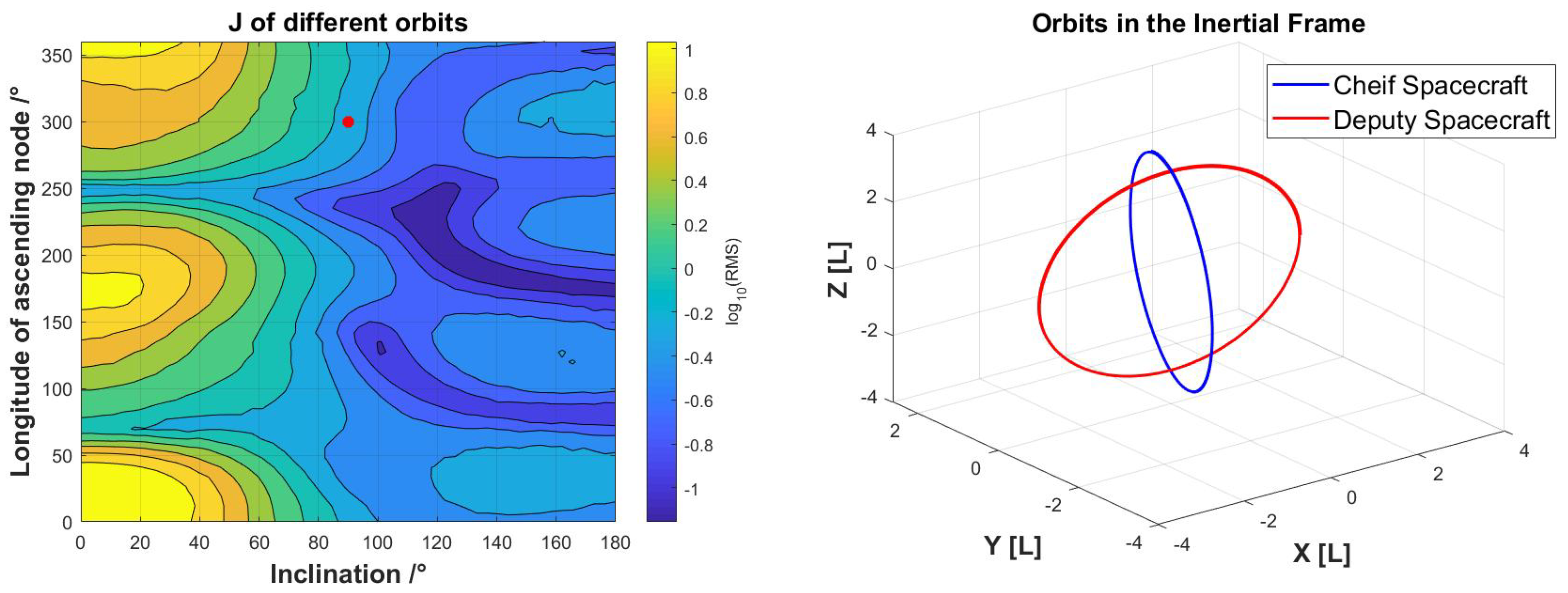
For the deputy, we set $a=3\left[L\right]$, $e=0$, $\omega =0^{\circ }$ and $M=0^{\circ }$, and we changed the values of its longitude of ascending node $\mathrm{\Omega }$ and orbit inclination i to study the sensitivity of the inter-satellite range data to its orbital plane. Left frame of Figure 1 displays the contour maps of measurement sensitivity when different values of orbit inclinations and longitude of ascending node are chosen.The abscissa is the orbit inclination of the deputy, and the ordinate is the difference in the longitude of the ascending node between the chief and the deputy. The sensitivity index is calculated using the following equation

$$\mathbf{J}=\sqrt{\frac{\sum {({\rho }_i^{\prime }-{\rho }_i)}^2}{n}}$$

(5)

where n is the number of measurements. ${\rho }_i$ is the inter-satellite range data when the gravity filed in Table 1 was adopted, and ${\rho }_i^{\prime }$ is the inter-satellite range data with a small error (+${10}^{-3}$) added to the $C_{22}$ term. A measurement interval of 0.05(T) and an arc length of 100(T) are taken for Figure 1, where (T) is the Unit time shown in Table 2.

From the left frame of Figure 1, we find that with the increase in the orbit inclinations, the measurement sensitivity $\mathbf{J}$ decreases. In addition, there is a periodic patten in the contour map when different values of the longitude of the ascending node are taken. It seems that the maximum sensitivity happens when the deputy’s $\mathrm{\Omega }$ is close to the $\mathrm{\Omega }$ value of the chief. Only judging from Figure 1, we should choose prograde orbits ($i<{90}^{\circ }$) for the deputy. However, due to the instability of the prograde orbit, the deputy may quickly collide with the asteroid. In such a case, we are unable to obtain measurement data long enough. Therefore, in our study, we choose the orbit of the deputy as a polar orbit. This type of orbit is relatively stable, and receives enough influence from the asteroid’s non-spherical gravity. In this case, we set the deputy’s longitude of ascending node as $\mathrm{\Omega }=0^{\circ }$, shown as the red point in Figure 1. In addition, the orbit of the chief and the deputy are shown in the left frame of Figure 1.

3. Sub-Problem 1

Sub-problem 1 is the orbit determination with prescribed gravity-field coefficients. As mentioned in Section 1, the highly irregular non-spherical gravity makes it possible to determine the autonomous orbit using only the inter-satellite range data. In this section, for the gravity field listed in Table 1, we use several examples to demonstrate the feasibility.

3.1. The Batch Algorithm

For each measurement, the residual y is expressed as:

$$y_i=Y_{oi}-Y_{ci}$$

(6)

where the subscript ‘c’ indicates the calculated value, and the subscript ‘o’ indicates the measured value. The subscript i is the serial number of measurement. Y is the measurement data. Here, it is the same as Equation (3). For a constellation of two spacecraft, the state vector (denoted as ${\mathbf{X}}_{\mathbf{0}}$) to be determined is a 12-dimensional vector which includes the position and velocity of both spacecrafts. The error in the initial state vector is denoted as $\widehat{x_0}$. The equation of orbit determination becomes

$$y_i=H_x{\widehat{x}}_0+ϵ$$

(7)

where

$$H_x=\frac{\partial Y_i}{\partial X_i}\frac{\partial X_i}{\partial X_0}=\widetilde{H_x}\mathrm{\Phi };\mathrm{\Phi }=\frac{\partial X_i}{\partial X_0}$$

(8)

$\mathrm{\Phi }$ is the system transition matrix calculated by integrating the following equation

$$\dot{\mathrm{\Phi }}(X,t)=\frac{\partial \dot{X}}{\partial X}\mathrm{\Phi }(X,t)$$

(9)

Using the batch algorithm [22], the solution of ${\widehat{x}}_0$ can be estimated as

$${\widehat{x}}_0={\left(H_x^T{H}_x\right)}^{-1}{H}_x^{T}y$$

(10)

By substituting Equation (10) into the initial estimate of the state vector ${\mathbf{X}}_0$, we can start the iteration process until the correction $\widehat{x_0}$ is small enough. This is a common practice in orbit determination and further details are omitted.

Detailed expression of $\widetilde{H_x}$ in Equation (8) depends on the type of the measurement data. For the inter-satellite range data, it can be expressed as

$$\widetilde{H_x}=\frac{\partial Y}{\partial X}=[\frac{x}{\rho },\frac{y}{\rho },\frac{z}{\rho },0,0,0,-\frac{x}{\rho },-\frac{y}{\rho },-\frac{z}{\rho },0,0,0]$$

(11)

where $x,y,z$ are given in Equation (2).

3.2. Two Examples

In this section, two examples are shown to demonstrate the feasibility of autonomous orbit determination using only the inter-satellite range data. In the tests, only two spacecrafts and one link are considered. The initial orbital elements are ${\sigma }_1=[3,0,{90}^{\circ },{60}^{\circ },{60}^{\circ },0^{\circ }]$ and ${\sigma }_2=[3,0,0^{\circ },0^{\circ },0^{\circ },0^{\circ }]$. For the initial estimation, a random error (with a threshold of 100 m) along all three directions is added to the position vector of both the chief and the deputy. The measurement interval is 0.05(T). The only difference between the two tests is the arc length used for orbit determination. It is 50(T) for test 1 and 100(T) for test 2. The result is shown in Figure 2. The left frame shows the residual in the observation data, and the right frame shows the position errors of the determined orbit with respect to the true one. The blue line is the position error of satellite 1 and the red line is the position error of satellite 2.

For test 1, the residual of the observation reaches the accuracy level of the observation data, and the position errors are smaller than 0.4 m. For test 2, where the arc length is longer, both the residual in the observation data and the position errors increase when compared with test 1. The reason for this phenomenon is that the force model for the orbit determination is different from the ’real’ force model which we use to generate the simulated observation data. When the length is too long, the difference between the two force models will cause the decrease of accuracy. To find an appropriate arc length, we conducted some further tests and displayed the relationship of the $RMS$ with respect to the arc length in Figure 3. The abscissa is the arc length, and the ordinate is the $RMS$ of the residuals. $RMS$ is calculated by the following equation

$$RMS=\sqrt{\frac{\sum {({\rho }_i^{\prime }-{\rho }_i)}^2}{n}}$$

(12)

Different from Equation (5), here ${\rho }^{\prime }$ is the calculated value and $\rho$ is the observed value.

From Figure 3, the accuracy of $RMS$ is the best with 40(T) to 80(T) arc length. When the arc length is larger than 80(T), the accuracy decreases quickly. By our calculation, for most cases, the arc of 50(T) is sufficient.

4. Sub-Problem 2

Sub-problem 2 is the gravity-field recovery with stable initial orbital elements. In Section 3, the feasibility of autonomous orbit determination was demonstrated by assuming that the asteroid’s gravity field is known a priori. In this section, we demonstrate the feasibility of the other sub-problem. That is the feasibility of gravity-field recovery from inter-satellite range data by assuming that the orbits of the two spacecraft are known a priori.

4.1. The Batch Algorithm

We define the gravity-field coefficients to be determined as C, and the error of the coefficients as $\widehat{c}$. Considering errors in other coefficients, Equation (7) can be reformulated as

$$y_i=H_x\widehat{x_0}+H_c\widehat{c}+ϵ$$

(13)

where

$$H_c=\frac{\partial Y_i}{\partial X_i}\frac{\partial X_i}{\partial C}=\widetilde{H_x}{\mathrm{\Phi }}_c;{\mathrm{\Phi }}_c=\frac{\partial X_i}{\partial C}$$

(14)

${\mathrm{\Phi }}_c$ is the sensitivity matrix, which can be calculated by integrating the following equation

$$\dot{{\mathrm{\Phi }}_c}(X,t)=\frac{\partial \dot{X}}{\partial X}{\mathrm{\Phi }}_c(X,t)+\frac{\partial \dot{X}}{\partial C}$$

(15)

Similar to Equation (10), $\widehat{c}$ can be estimated by the following formula if we assume no error to the initial state vector ${\mathbf{X}}_0$.

$$\widehat{c}={\left(H_c^T{H}_c\right)}^{-1}{H}_c^{T}y$$

(16)

Same as the orbit determination process, the process to determine the gravity-field coefficients should be repeated until the correction $\widehat{c}$ is small enough.

4.2. Feasibility Analysis

The first question to be answered is whether the gravity-field recovery is possible with the inter-satellite range data. To answer this question, we remove errors from the simulated observation data, i.e, the observations are accurate. We compute the residuals as functions of the gravity coefficients $C_{20}$ and $C_{22}$ to be determined. We also assume that the orbits are already determined without errors, and the initial conditions for the two orbits are the same as test 1 in Section 3.2: ${\sigma }_1=[3,0,{90}^{\circ },{60}^{\circ },{60}^{\circ },0^{\circ }]$ and ${\sigma }_2=[3,0,0^{\circ },0^{\circ },0^{\circ },0^{\circ }]$. For the example orbits above, the $RMS$ as a function of $C_{20}$ and $C_{22}$ is displayed in the contour map, Figure 4a. There is no doubt that there is only a single minimum in the contour map, which indicates that the gravity-field recovery is possible, in theory. The integration time is 100(T) and the measurement interval is 0.05(T).

There is only one global minimum value of the RMS, so it is possible for us to achieve the gravity-field recovery. However, if the measurements are too sparse, the number of local optimum will be more than one. In Figure 4b, the measurement interval is set as 1(T). Obviously, there is more than one local minimum value in Figure 4b. In this case, it is difficult to recover the accurate gravity field. Therefore, dense measurement data is recommended for the gravity-field recovery. For this reason, in the calculations below, the measurement interval is set as 0.05(T).

Here is an example. The initial conditions are the same as the example in Section 3.2. The initial estimate of gravity-field coefficients is $C_{20}=-5\times {10}^{-2}$ and $C_{22}=9\times {10}^{-2}$ and the measurement interval is set as 0.05(T). The recovered gravity-field coefficients are

$$C_{20}=-5.247792\times {10}^{-2};C_{22}=8.253777\times {10}^{-2}$$

(17)

Compared with Table 1, the result is very close to the true value $C_{20}=-5.2478\times {10}^{-2}$ and $C_{22}=8.2538\times {10}^{-2}$.

4.3. Influence of Observation Error

In practice, there are errors in the determined orbits. In this situation, the relationship between the residual and the $C_{20}$ and the $C_{22}$ term will be different. In this example, we set the position error of both the chief and the deputy as 10 m in all the three directions randomly. Using the same approach as in Figure 4, the result is shown in Figure 5.

In this example case, there is still only one global optimal value. In other words, the recovery calculation is still feasible. Using the same initial conditions as in Figure 5, the result is

$$C_{20}=-5.326190\times {10}^{-2};C_{22}=8.480794\times {10}^{-2}$$

(18)

The accuracy is worse than the result in Equation (17), and the accuracy is speculated to be even worse if larger errors in the determined orbits exist. This phenomenon poses a considerable challenge to the following complete inverse problem where both orbit determination and gravity-field recovery are required simultaneously.

5. The Complete-Inverse Problem

In Section 3 and Section 4.2, we showed the feasibility of the two sub-problems, respectively. However, the feasibility of the two sub-problems cannot guarantee the feasibility of the complete-inverse problem. In this case, the gravity field and orbit are coupled, and we need to estimate the orbit and gravity field together.

In our work, the mutual influence between the two sets of parameters (the gravity field and the orbits) is so strong that it is hard to converge. When the error of the initial estimate is too large, the complete-inverse problem is hard to converge. To solve this problem, we use the adaptive step size to control in the iteration process. As shown in Equation (19).

$$\tilde{x}=\frac{\widehat{x}}{1+k|\widehat{x}|}$$

(19)

$\widehat{x}=[{\widehat{x}}_0,\widehat{c}]$ is the calculated correction value by the iteration process. It is quite possible that $\widehat{x}$ is too large. Directly correcting the estimate with this calculated value may lead to a worse estimate and eventually the failure of the iteration process. To overcome this problem, we deliberatively decrease the size of the correction value by introducing the step-size control parameter k. $\tilde{x}$ is the actual correction value taken and k is an empirical constant which usually takes the value of 1. In such a case, when $\widehat{x}$ is large (i.e., the estimate is far from the true value), the size of the actual correction $|\tilde{x}|$ is always smaller than 1. When $\widehat{x}$ is small (i.e., the estimate is close to the true value), $\tilde{x}\approx \widehat{x}$.

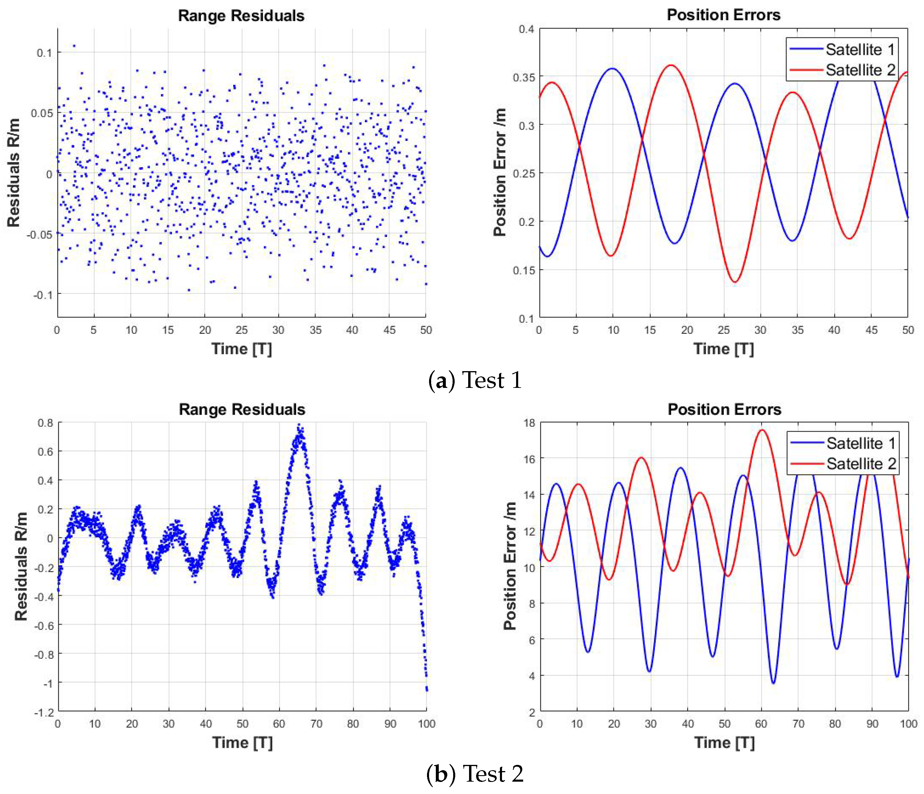
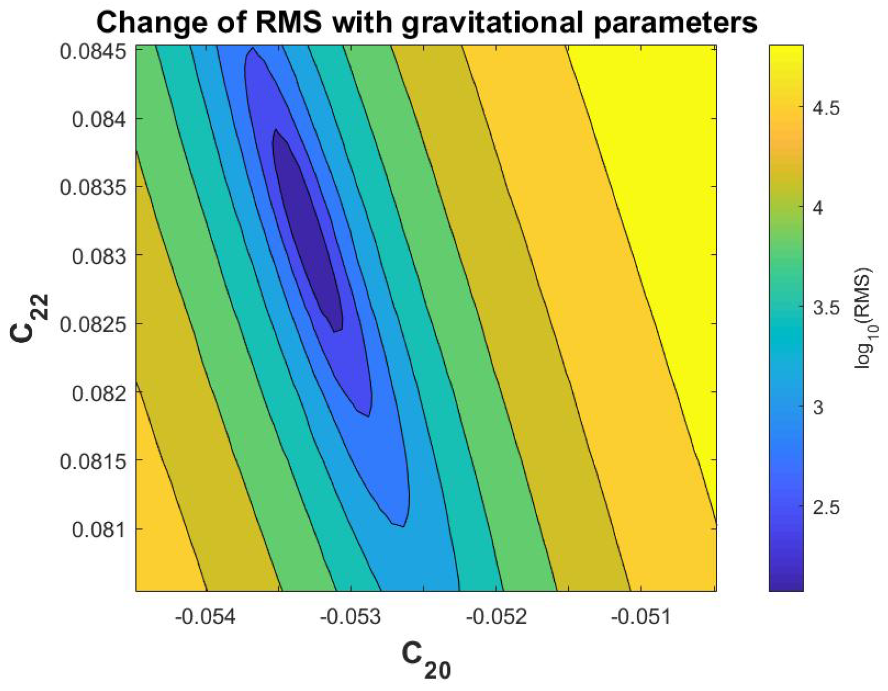
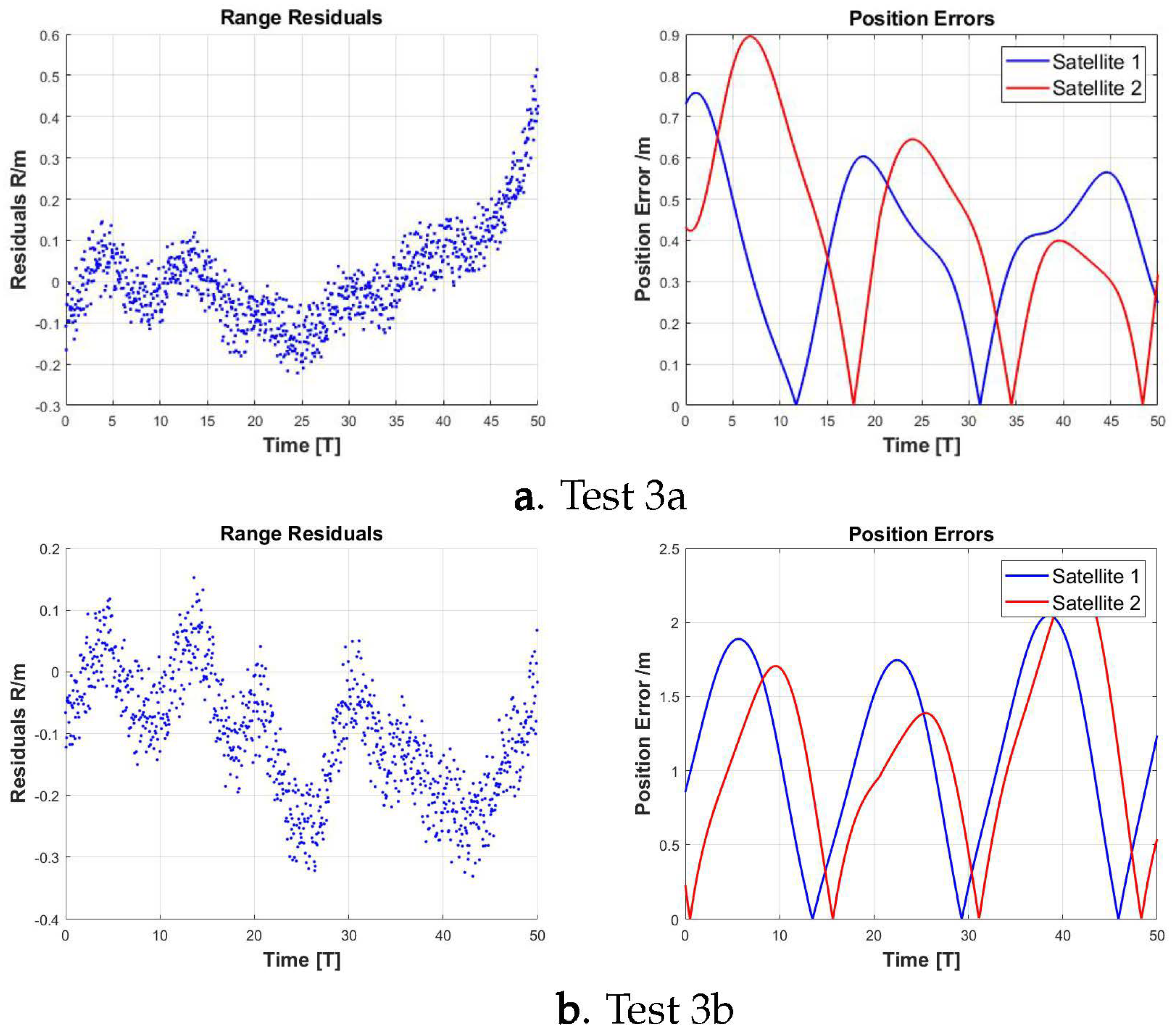
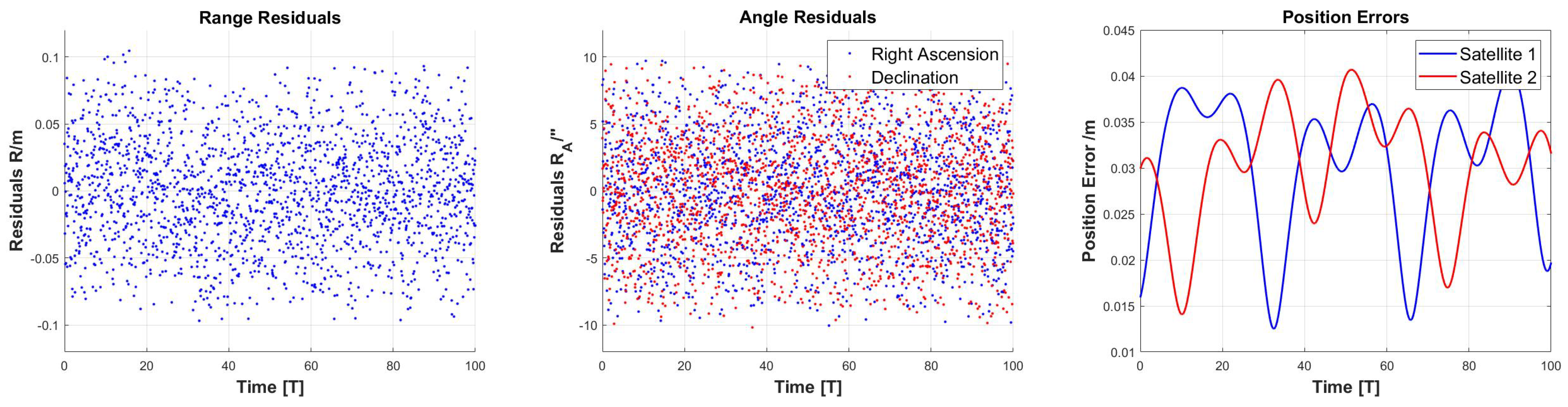
Test 3 shows two examples with good initial estimates. The simulation observation data of them are the same: The initial position is the same as Section 3.2. But the initial estimate of initial position is different. Random error (with a threshold of 10 m) along all three directions is added differently in the two examples. The initial estimate of the gravity field is the same, where $C_{20}=-5.20\times {10}^{-2}$ and $C_{22}=8.30\times {10}^{-2}$. For an arc length of 50(T), the result is shown in Figure 6 and

Table 3. Recovery result of test 3.

Parameter	Initial Estimate	Test 3.a	Test 3.b
$C_{20}$	$-5.20\times {10}^{-2}$	$-5.2467\times {10}^{-2}$	$-5.2309\times {10}^{-2}$
$C_{22}$	$8.30\times {10}^{-2}$	$8.2559\times {10}^{-2}$	$8.2455\times {10}^{-2}$
Initial position error of Satellite 1	10 m	0.75 m	0.90 m
Initial position error of Satellite 2	10 m	0.43 m	0.24 m

. And

Table 4. The change of RMS in test 3.

RMS	Test 3.a	Test 3.b
Initial Estimate	6.4053	8.0739
Result	0.1167	0.1417

reflects the change of RMS for two examples before and after the calculation.

Obviously, the results after iteration are much better than the initial estimate. For test 3a, the residuals of observation are less than 0.5 m, and the position errors of estimated orbits are less than 0.8 m. For test 3b, the residuals are less than 0.3 m and the position errors are less than 2 m. In addition, the difference in the results of these two tests is small. The accuracy of the estimated gravity-field coefficients is about $0.02\%$ for test 3a and about $0.1\%$ for test 3b. The RMS of them are similar. Thus, we can say that the orbit determination process has converged.

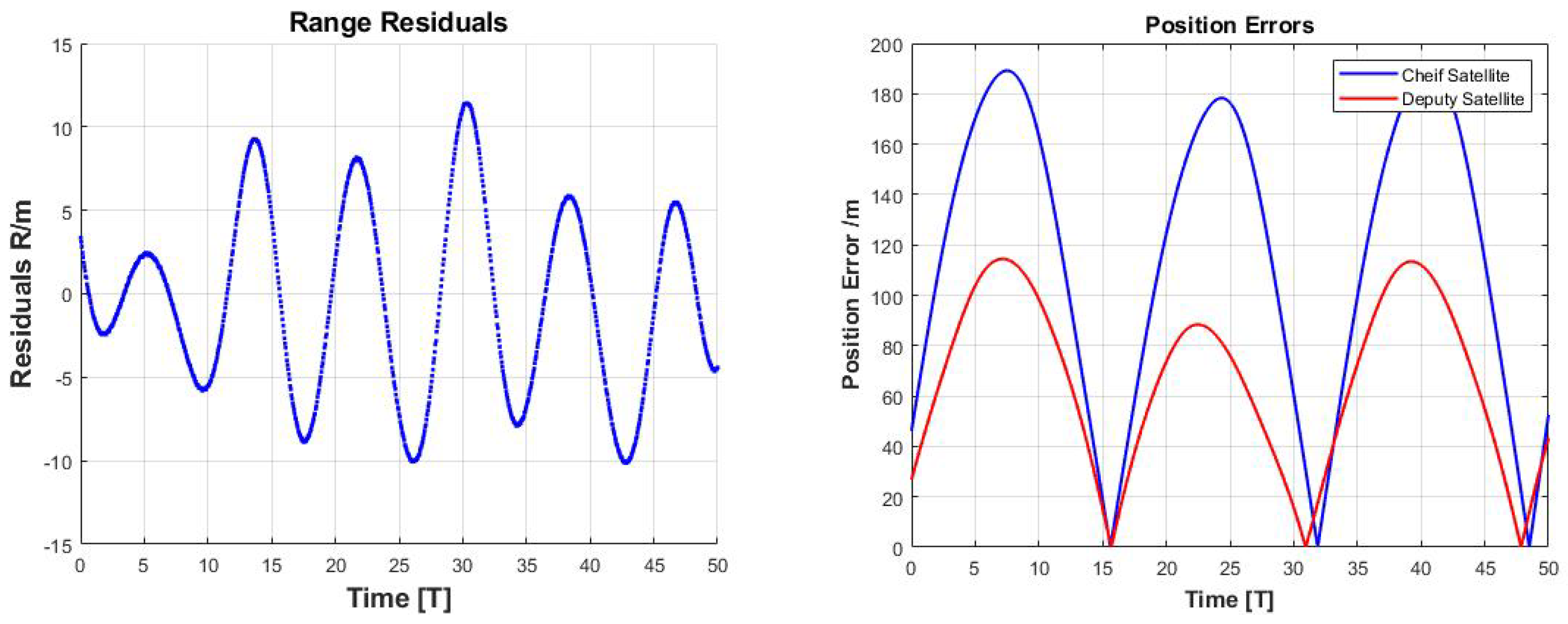
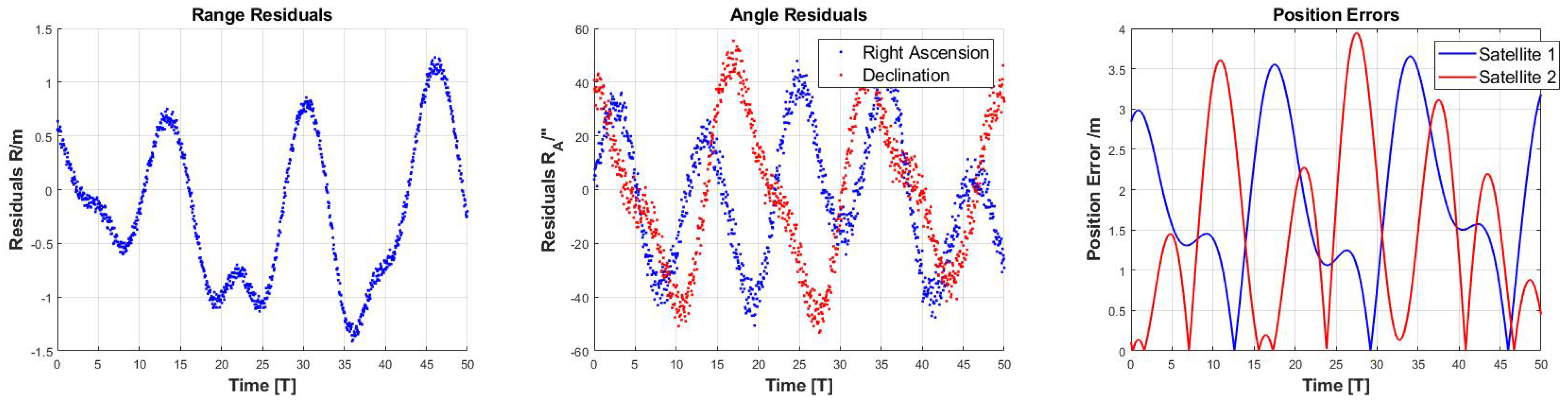
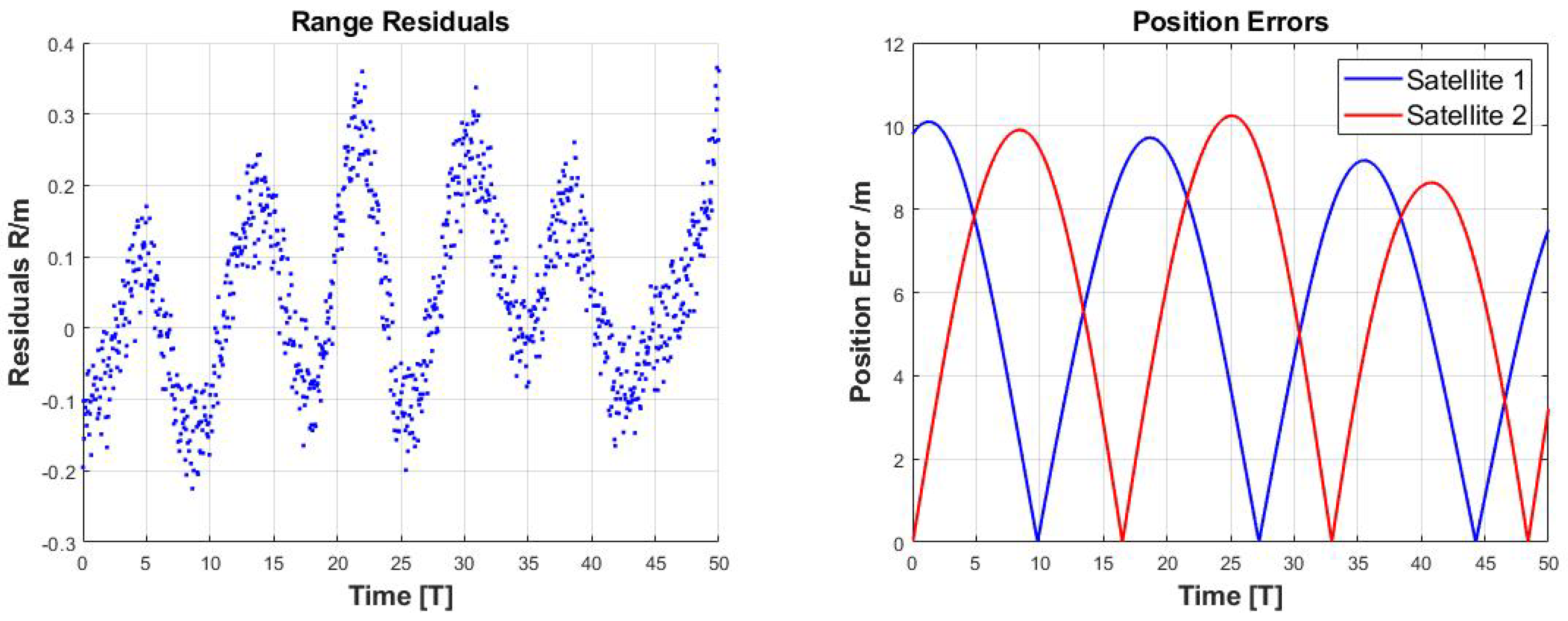
However, when the initial estimate is poor, the iteration process converges harder, and the accuracy of the results obviously decreases. In test 4, we randomly added a position error of 50 m in all the three directions of both the spacecraft. The initial estimate of the gravity-field coefficients are $C_{20}=-5\times {10}^{-2}$ and $C_{22}=9\times {10}^{-2}$. Setting the arc length as 50(T), the result is shown in Figure 7 and

Table 5. Recovery result of test 4.

Parameter	Initial Estimate	Test 4
$C_{20}$	$-5\times {10}^{-2}$	$-5.3959\times {10}^{-2}$
$C_{22}$	$9\times {10}^{-2}$	$7.5978\times {10}^{-2}$
Initial position error of Satellite 1	50 m	47.71 m
Initial position error of Satellite 2	50 m	27.67 m
RMS	39.9917	5.5752

.

Figure 7 and Table 5 indicate that the iteration process has not converged, because some of the final result is even worse than the initial estimates.

Studies in this section demonstrate the feasibility of the complete-inverse problem. However, a good initial guess is necessary for the convergence of the problem. In order to obtain a good initial estimate, we tried to use the particle swarm optimization method (PSO) to find the global optimal solution. However, most of the time, the PSO fails to converge or converges to a local minimum far away from the true value. Thus, this attempt failed. In the following, we propose two improved algorithms to help solve the narrow convergence-region problem.

6. Discussion

6.1. Two Improved Algorithms

6.1.1. Multiple Links

In this case, more than one link is used. We choose one of these spacecrafts as the chief spacecraft, and the others as the deputy spacecraft. Using multi-spacecraft constellation, the convergence region of the problem can be extended.

Figure 8 shows an example (test 5). It is a constellation with one chief spacecraft and eight deputy spacecrafts. In this case, we put the deputy spacecraft in different types of orbits to obtain stronger signals from the non-spherical gravity. By our calculation, the spacecraft of prograde orbit do not collide with the asteroid for a 50(T) arc length. Thus, we put the chief spacecraft in the polar orbit (the black trajectory in the right picture of Figure 8, the orbital elements are the same as ${\sigma }_1$ in Section 3.2). Four of the deputy spacecrafts are in the prograde orbits (the blue trajectories) and four of them are in the polar orbits (the red trajectories). The initial position error is set as 50 m (the same as test 4) randomly along all three directions of all the spacecraft. For the initial estimation, an error of 50 m is randomly added in all the three directions to the position vector of the chief and all of the deputy, respectively. Initial estimate of the gravity-field coefficients is $C_{20}=-5\times {10}^{-2}$ and $C_{22}=9\times {10}^{-2}$ (

Table 6. Recovery result of test 5.

Parameter	Initial Estimate	Test 4
$C_{20}$	$-5\times {10}^{-2}$	$-5.0871\times {10}^{-2}$
$C_{22}$	$9\times {10}^{-2}$	$8.2667\times {10}^{-2}$
Initial position error of Chief Satellite	50 m	20.12 m

). Our test shows that the complete-inverse problem converges well in this example.

Unlike test 4, the result after iteration is better than the initial estimate, so the iteration process has converged. Most of the residuals are less than 10 m and position errors of estimated orbits are less than 50 m. In addition, the value of $C_{22}$ is much better than test 4. The error is only 0.15%. This improvement in this result is significant. As a feasibility analysis, test 5 is enough. It can prove that more links can extend the convergence region.

6.1.2. The Addition of Inter-Satellite Angle Data

The Osiris-Rex mission uses the angle-measurement data from the spacecraft to the particles near Bennu’s surface to recover the asteroid’s gravity to high orders and degrees [10]. Inspired by this, we added the inter-satellite angle measurement data into our study as a supplementary to the inter-satellite range data to improve the accuracy.

For inter-satellite angle data, $\widetilde{H_x}=[\frac{\partial \delta }{\partial X},\frac{\partial \alpha }{\partial X}]$ will be

$$\frac{\partial \delta }{\partial X}=[{\delta }_x,{\delta }_y,-{\delta }_Z,0,0,0,-{\delta }_x,-{\delta }_y,{\delta }_Z,0,0,0]$$

(20)

$$\frac{\partial \alpha }{\partial X}=[\frac{y}{x^2+y^2},-\frac{x}{x^2+y^2},0,0,0,0,-\frac{y}{x^2+y^2},\frac{x}{x^2+y^2},0,0,0,0]$$

(21)

where ${\delta }_x$, ${\delta }_y$ and ${\delta }_z$ can be calculated using Equation (22).

$${\delta }_x=\frac{xz}{{\rho }^3\sqrt{1-{(z/\rho )}^2}}{\delta }_y=\frac{yz}{{\rho }^3\sqrt{1-{(z/\rho )}^2}}{\delta }_z=\frac{1}{\sqrt{1-{(z/\rho )}^2}}(\frac{1}{r}-\frac{z^2}{{\rho }^3})$$

(22)

Firstly, our study indicates that the addition of the inter-satellite angle measurement data can significantly improve the accuracy of the orbit determination. As test 6 (Figure 9) shows, all of the initial conditions are the same as those of test 2 in Section 3.2.

Compared with test 2, the accuracy of test 6 is much better. The range residuals are less than 0.1 m and the angle residuals are less than 10 arc-seconds. Both of them reach the accuracy level of observation data, just like test 1. The position errors of test 6 are less than 0.04 m and the position errors of test 2 are about 14 m. Thus, it is clear that the addition of angle data can provide more constraints to improve the accuracy.

When both initial orbital elements and gravity-field coefficients are erroneous, the addition of angle measurement data also works. In test 7, all of the initial conditions are the same as test 4 in Section 5 and the result is shown in Figure 10 and

Table 7. Recovery result of test 7.

Parameter	Initial Estimate	Test 4
$C_{20}$	$-5\times {10}^{-2}$	$-5.4093\times {10}^{-2}$
$C_{22}$	$9\times {10}^{-2}$	$8.2626\times {10}^{-2}$
Initial position error of Satellite 1	50 m	2.89 m
Initial position error of Satellite 2	50 m	0.08 m
RMS	39.9917	5.5752

.

Similarly to test 5, the accuracy of result has improved a lot. The range residuals are about one meter and the angle residuals are about 40 arc-seconds. Position errors are only 3.5 m and the initial errors are less than 3 m. The value of gravity-field coefficients is close to the real value. Their errors are $3\%$ and $0.1\%$, respectively. Compared with test 4, this result is excellent. The improvement in accuracy is significant.

In addition, from the above results, we can find that the accuracy of the tesseral $C_{22}$ term is much better than the zonal $C_{20}$ term. It is due to the fact that the influence of the tesseral harmonic $C_{22}$ is much greater than the zonal harmonic $C_{20}$ in the calculation of gravity-field recovery.

6.2. The Influence of SRP

Furthermore, let us consider the influence of the other perturbation. As mentioned in Section 2, SRP is the largest perturbation besides the non-spherical gravity. In test 8, the influence of the SRP is considered in the simulated measurement data. In addition, we still only consider the second non-spherical gravity in the orbit determination. Here, because the value of SRP is relatively small, we use a simple model. It can be expressed as [21].

$$F_{SRP}=\rho (1+\eta )\frac{S}{m}\frac{\mathbf{r}}{r}$$

(23)

where $\rho$ is the solar radiation pressure at r, $\eta$ is the spacecraft’s reflectance, $S/m$ is the spacecraft’s area to mass ratio and r is the spacecraft position vector to the sun. We set $\eta$ as 0.5 and $S/m$ as 0.01. The initial conditions are identical to test 3: The position errors of both the spacecraft are set as 10 m in all three directions randomly and the initial estimate of the gravity field is $C_{20}=-5.20\times {10}^{-2}$ and $C_{22}=8.30\times {10}^{-2}$. For an arc length of 50(T), the result is shown in Figure 11 and

Table 8. Recovery result of test 8.

Parameter	Initial Estimate	Test 4
$C_{20}$	$-5.20\times {10}^{-2}$	$-5.2475\times {10}^{-2}$
$C_{22}$	$8.30\times {10}^{-2}$	$8.2476\times {10}^{-2}$
Initial position error of Satellite 1	10 m	9.88 m
Initial position error of Satellite 2	10 m	0.14 m
RMS	8.1752	0.1306

.

For test 8, the residuals of observation are less than 0.3 m and the position error is less than 10 m. The accuracy of the gravity field is about 0.07%. Compared with test 3, the accuracy of the result is similar. It also demonstrates that the other perturbations, such as SRP, only have little influence in our case since we have a large asteroid.

7. Conclusions

In this work, we mainly demonstrated the feasibility of orbit determination and gravity-field recovery using only inter-satellite range data in three steps. First, sub-problem 1, in which the gravity field is known a priori and the orbits of the chief and the deputy are autonomously determined, is studied. Second, sub-problem 2, in which the orbits of the chief and the deputy are known a priori and the gravity field is recovered, is studied. Then, the complete-inverse problem in which both the orbits of the chief and the deputy and the gravity field are determined is studied. Our study shows that the complete-inverse problem is invertible, but the convergence region is very narrow, i.e., an initial estimate close to the real one is necessary. Two improved algorithms are proposed to solve this problem: using multiple links by adding more deputies and adding the angle measurement data between the chief and deputies. By our calculation, both algorithms can increase the convergence region and improve the accuracy. Our studies find that the accuracy of the zonal $C_{20}$ term is worse than the accuracy of the tesseral $C_{22}$ term. In addition, we also analyzed the influence of different orbit types on the inter-satellite range data and the influence of different arc lengths on the orbit determination.

We need to stress that this work is only a feasibility study. Our conclusions are based on some assumptions. For asteroids of hundreds of meters in size or smaller, it is possible that SRP is one order of magnitude larger than non-spherical gravity which may seriously challenge the assumptions in the current study. The study indicates that it is possible to solve the complete inverse problem using only the inter-satellite range data, but a good initial estimation is necessary and the accuracy of the results is limited. A more realistic mission scenario is to combine the accurate inter-satellite range data along with ground observation data to do the complete inverse problem. We are currently working on this project.

References

1. Miller, J.K.; Konopliv, A.S.; Antreasian, P.G.; Bordi, J.J.; Chesley, S.; Helfrich, C.E.; Owen, W.M.; Wang, T.C.; Williams, B.G.; Yeomans, D.K.; et al. Determination of Shape, Gravity, and Rotational State of Asteroid 433 Eros. Icarus 2002, 155, 3–17. [Google Scholar] [CrossRef]
2. Konopliv, A.S.; Asmar, S.W.; Park, R.S.; Bills, B.G.; Centinello, F.; Chamberlin, A.B.; Ermakov, A.; Gaskell, R.; Rambaux, N.; Raymond, C.; et al. The Vesta gravity field, spin pole and rotation period, landmark positions, and ephemeris from the Dawn tracking and optical data. Icarus 2014, 240, 103–117. [Google Scholar] [CrossRef]
3. Konopliv, A.S.; Park, R.S.; Vaughan, A.T.; Bills, B.G.; Asmar, S.W.; Ermakov, A.I.; Rambaux, N.; Raymond, C.A.; Castillo-Rogez, J.C.; Russell, C.T.; et al. The Ceres gravity field, spin pole, rotation period and orbit from the Dawn radiometric tracking and optical data. Icarus Int. J. Sol. Syst. Stud. 2018, 299, 411–429. [Google Scholar] [CrossRef]
4. Cao, J.; Hu, S.; Liu, L.; Liu, Y.; Huang, Y.; Li, P. Orbit determination and analysis for Chang’E-2 asteroid exploration. J. Bjing Univ. Aeronaut. Astronaut. 2014, 40, 1095–1101. [Google Scholar]
5. Curkendall, D.W.; Border, J.S. Delta-DOR: The One-Nanoradian Navigation Measurement System of the Deep Space Network—History, Architecture, and Componentry. Int. J. Mol. Sci. 2013, 5, 1. [Google Scholar]
6. Leonard, J.M.; Antreasian, P.G.; Jackman, C.D.; Page, B.; Wibben, D.R.; Moreau, M.C. Orbit Determination Strategy and Simulation Performance for OSIRIS-REx Proximity Operations. In Proceedings of the International ESA Conference on Guidance, Navigation and Control Systems, Copely Plaza, MA, USA, 29 May–2 June 2017. [Google Scholar]
7. Williams, B.; Antreasian, P.; Carranza, E.; Jackman, C.; Leonard, J.; Nelson, D.; Page, B.; Stanbridge, D.; Wibben, D.; Williams, K.; et al. OSIRIS-REx Flight Dynamics and Navigation Design. Space Sci. Rev. 2018, 214, 69. [Google Scholar] [CrossRef]
8. Werner, R.A.; Scheeres, D.J. Exterior gravitation of a polyhedron derived and compared with harmonic and mascon gravitation representations of asteroid 4769 Castalia. Celest. Mech. Dyn. Astron. 1996, 65, 313–344. [Google Scholar] [CrossRef]
9. Zhao, Y.; Yang, H.; Li, S.; Zhou, Y. On-board modeling of gravity fields of elongated asteroids using Hopfield neural networks. Astrodyn 2023, 7, 101–114. [Google Scholar] [CrossRef]
10. Park, R.S.; Konopliv, A.S.; Asmar, S.W.; Bills, B.G.; Gaskell, R.W.; Raymond, C.A.; Smith, D.E.; Toplis, M.J.; Zuber, M.T. Gravity field expansion in ellipsoidal harmonic and polyhedral internal representations applied to Vesta. Icarus 2014, 240, 118–132. [Google Scholar] [CrossRef]
11. Tricarico, P.; Scheeres, D.J.; French, A.S.; McMahon, J.W.; Brack, D.N.; Leonard, J.M.; Antreasian, P.; Chesley, S.R.; Farnocchia, D.; Takahashi, Y.; et al. Internal rubble properties of asteroid (101955) Bennu. Icarus 2021, 370, 114665. [Google Scholar] [CrossRef]
12. Ledbetter, W.G.; Sood, R.; Keane, J.; Stuart, J. SmallSat swarm gravimetry: Revealing the interior structure of asteroids and comets. Astrodyn 2021, 5, 217–236. [Google Scholar] [CrossRef]
13. Park, R.; Konopliv, A.; Bills, B.; Rambaux, N.; Castillo-Rogez, J.C.; Raymond, C.A.; Vaughan, A.T.; Ermakov, A.I.; Zuber, M.T.; Fu, R.R.; et al. A partially differentiated interior for (1) Ceres deduced from its gravity field and shape. Nature 2016, 537, 515–517. [Google Scholar] [CrossRef] [PubMed]
14. Chesley, S.R.; French, A.S.; Davis, A.B.; Jacobson, R.A.; Brozović, M.; Farnocchia, D.; Selznick, S.; Liounis, A.J.; Hergenrother, C.W.; Moreau, M.C.; et al. Trajectory estimation for particles observed in the vicinity of (101955) Bennu. Geophys. Res. Planets 2020, 125, e2019JE006363. [Google Scholar] [CrossRef]
15. Lauretta, D.S.; Hergenrother, C.W.; Chesley, S.R.; Leonard, J.M.; Pelgrift, J.Y.; Adam, C.D.; Al Asad, M.; Antreasian, P.G.; Ballouz, R.-L.; Becker, K.J.; et al. Episodes of particle ejection from the surface of the active asteroid (101955) Bennu. Science 2019, 366, eaay3544. [Google Scholar] [CrossRef]
16. Zhou, W.; Gao, W.; Lin, X.; Hu, X.; Ren, Q.; Tang, C. Emerging errors in the orientation of the constellation in GNSS autonomous orbit determination based on inter-satellite link measurements. Adv. Space Res. 2022, 70, 3156–3172. [Google Scholar] [CrossRef]
17. Fernandez, F.A. Inter-satellite ranging and inter-satellite communication links for enhancing GNSS satellite broadcast navigation data. Adv. Space Res. 2011, 47, 786–801. [Google Scholar] [CrossRef]
18. Tang, C.; Hu, X.; Zhou, S.; Liu, L.; Pan, J.; Chen, L.; Guo, R.; Zhu, L.; Hu, G.; Li, X.; et al. Initial results of centralized autonomous orbit determination of the new-generation BDS satellites with inter-satellite link measurements. J. Geod. 2018, 92, 1–15. [Google Scholar] [CrossRef]
19. Kang, Z.; Bettadpur, S.; Nagel, P.; Save, H.; Poole, S.; Pie, N. GRACE-FO precise orbit determination and gravity recovery. J. Geod. 2020, 94, 84–100. [Google Scholar] [CrossRef]
20. Vetrisano, M.; Vasile, M. Autonomous navigation of a spacecraft formation in the proximity of an asteroid. Adv. Space Res. 2015, 57, 1783–1804. [Google Scholar] [CrossRef] [Green Version]
21. Scheeres, D.J. Orbital mechanics about small bodies. Acta Astronaut. 2012, 72, 1–14. [Google Scholar] [CrossRef]
22. Tapley, B.D.; Schutz, B.E.; Born, G.H. Statistical Orbit Determination. Stat. Orbit Determ. 2004, 39, 159–284. [Google Scholar]
Figure 1. Contour map of measurement index J with 10 3 error in C 22 (left) and Orbit of the chief spacecraft and the deputy spacecraft (right).
Aerospace 10 00304 g001
Figure 2. Residual in the observation data (left) and norm of the position error of the determined orbit from the true one (right).
Aerospace 10 00304 g002
Figure 3. R M S of different arc lengths.
Aerospace 10 00304 g003
Figure 4. Contour map of the residual with respect to the gravity-field coefficients C 20 and C 22 (accuracy initial position). (a) Contour map of a 0.05(T) measurement interval. (b) Contour map of a 1(T) measurement interval.
Aerospace 10 00304 g004
Figure 5. Contour map of the residual with respect to the gravity-field coefficients C 20 and C 22 (erroneous initial position).
Aerospace 10 00304 g005
Figure 6. Residual in the observation data (left) and norm of the position error of the determined orbit from the true one (right) (test 3 with small errors in the initial estimate).
Aerospace 10 00304 g006
Figure 7. Residual in the observation data (left) and norm of the position error of the determined orbit from the true one (right) (test 4 with large errors in the initial estimate).
Aerospace 10 00304 g007
Figure 8. Residual in the observation data (left), norm of the position error of the determined orbit from the true one (middle) and orbits of spacecraft (right) (test 5 with 8 links).
Aerospace 10 00304 g008
Figure 9. Residual in the range data (left), residual in the angle data (middle) and norm of the position error of the determined orbit from the true one (right) (test 6).
Aerospace 10 00304 g009
Figure 10. Residual in the range data (left), residual in the angle data (middle) and norm of the position error of the determined orbit from the true one (right) (test 7).
Aerospace 10 00304 g010
Figure 11. Residual in the observation data (left) and norm of the position error of the determined orbit from the true one (right) (test 8).
Aerospace 10 00304 g011