Article

Makespan-Minimizing Heterogeneous Task Allocation under Temporal Constraints

1
Department of Aerospace Engineering, Korea Advanced Institute of Science and Technology, Daejeon 34141, Republic of Korea
2
School of Aerospace and Mechanical Engineering, Korea Aerospace University, Goyang 10540, Republic of Korea
3
Hanwha Systems Co., Seongnam 13524, Republic of Korea
*
Author to whom correspondence should be addressed.
Aerospace 2023, 10(12), 1032; https://doi.org/10.3390/aerospace10121032
Submission received: 17 November 2023 / Revised: 8 December 2023 / Accepted: 11 December 2023 / Published: 14 December 2023
(This article belongs to the Collection Unmanned Aerial Systems)

Abstract

:
Task allocation is an essential element for determining the capability of multi-UAV systems to perform various tasks. This paper presents a procedure called a “rebalancing algorithm” for generating task-performing routes in heterogeneous multi-UAV systems. The algorithm adopts a greedy-based heuristic approach to find solutions efficiently in dynamically changing environments. A novel variable named “loitering” is introduced to satisfy temporal constraints, resulting in improved performance compared to heuristic algorithms: a sequential greedy algorithm, a genetic algorithm, and simulated annealing. The rebalancing algorithm is divided into two phases to minimize the makespan, i.e., the initial allocation and reallocation phases. Simulation results demonstrate the proposed algorithm’s effectiveness in highly constrained conditions and its suitability for heterogeneous systems. Additionally, the results show a reduction in calculation time and improved performance compared to the heuristic algorithms.

1. Introduction

A multi-UAV (unmanned aerial vehicle) system refers to a group of multiple UAVs that work together to accomplish a common goal. The UAVs can be remotely controlled or operated autonomously, and they can perform their own tasks with simple directions. Recent advances in multi-UAV systems have focused on improving the coordination and autonomy of vehicles. When the paths for each UAV to perform tasks are predetermined, a task allocation method is not necessary. However, multi-UAV systems are being used in new ways, such as environmental monitoring [1], disaster response [2], and precision agriculture [3], for which tasks are presented with various constraints. Efficient task allocation methodologies can help properly derive the paths for performing the tasks under constraints.
Task assignment is a combinatorial optimization problem that is known to be NP-hard [4]. When task assignments involve constraints, the situation becomes significantly more challenging than when there are no restrictions on the assignments. A considerable amount of research has been conducted on the constrained task assignment problem. One study suggested an algorithm that generates solutions about task priorities and control inputs [5]. Decentralized approaches are also reviewed for asynchronous conditions [6], coupled constraints [7], cooperation constraints [8,9], and minimizing communication [10]. This problem is also solved by meta-heuristic methods like ant colony [11], genetic algorithm [12,13,14,15,16,17,18], particle swarm optimization [19], and simulated annealing [20,21,22,23,24].
The real-world mission scenario involves a heterogeneous multi-UAV system and a diverse set of tasks with varying characteristics and temporal constraints. Temporal constraints are typically applied to situations such as time-limited tasks or precedence conditions between two tasks. To address these temporal constraints, various methods have been developed and investigated. The market-based approach has yielded good results when dealing with temporally and spatially distributed tasks [25,26]. Iterated local search (ILS) is a method that complements the initial-value-dependent local search, and the ILS-based meta-heuristic algorithm shows robust results with regard to parameter tuning [27]. Also, much research about heterogeneous task allocation is performed. An optimal control approach [5] and a reinforcement learning approach [28] are suggested. The combination of the heterogeneity in multi-UAV systems and temporal constraints can make the problem particularly challenging due to its complexity.
This paper introduces a new variable, “loitering”, which is a term from aeronautics used to describe an air vehicle staying in the air while waiting for further direction. The proposed variable helps ensure that all constraints are satisfied in the task allocation process. Firstly, several algorithms are selected to solve the constrained task allocation problem, and the variable “loitering” is utilized to obtain feasible solutions. Next, a greedy-based heuristic algorithm, named the “rebalancing” algorithm, is proposed to generate paths for the heterogeneous multi-UAV system and to minimize the makespan of performing tasks while satisfying temporal constraints. In this paper, a path means the sequence of tasks performed by a UAV. The makespan is the total time to complete all given tasks by the UAVs in the system. The proposed algorithm is divided into two steps. In the first step, each task is allocated sequentially and greedily with evaluation for reward and penalty to form an initial path. In the second step, named “rebalancing”, a task is removed from the current path and reallocated to the most advantageous location, with a loitering time calculation used to determine if the new allocation is better than the original path. The proposed algorithm consisting of the initial allocation and rebalancing steps typically reduces makespan, and a more-balanced number of tasks is assigned to each UAV.
The structure of this paper is as follows. In Section 2, the problem statement is presented, which details the specific problem that is addressed in this paper. Section 3 outlines the calculation method of loitering time, which refers to the waiting time before initiating a task. Section 4 introduces the sequential greedy algorithm, genetic algorithm, and simulated annealing to solve task allocation problems using the calculation technique in Section 3. Section 5 explains the proposed rebalancing algorithm, which generates paths for each UAV and calculates a loitering time to satisfy all temporal constraints. Section 6 describes the various numerical simulation settings, results, and analyses. Finally, Section 7 concludes this paper.

2. Problem Statement

2.1. Heterogeneous Multi-UAV System and Temporal Constraints

This paper addresses the problem of allocating heterogeneous tasks to a heterogeneous multi-UAV system. The objective is to minimize the time required to complete all tasks, known as makespan, while ensuring that temporal constraints are satisfied. Different types of UAVs are considered, each with its own unique set of equipment and capabilities. For example, UAVs with cameras can be used for aerial photography and video, while those with depth cameras or LIDAR (light detection and ranging) can be used for creating digital elevation models for terrain, buildings, and other features. An illustrative example of compatibility is presented in Table 1. The value of 1 in cell (1,2) indicates that a UAV equipped with a thermal camera is capable of performing search tasks. On the other hand, the zero value in cell (4,1) tells that a UAV with a camera is supposed to be unable to perform mapping tasks.
The realistic situation consists of heterogeneous UAVs and tasks, as well as temporal constraints. One example of temporal constraints is a time-limited task. For instance, surveillance with a typical camera must be finished before sunset due to visibility. Another temporal constraint is a precedence condition between two tasks. For this, a delivery mission is a good example: a “Pickup” task must be performed before a “Delivery” task. Additionally, if a complex task needs multiple UAVs at the same time, it could be represented by a simultaneous constraint.
For more details, a representation of the time interval constraints is well organized in [29]. Temporal constraints on the relations between two tasks are represented in algebraic forms. For example, the constraint that task A should be finished before the beginning of task B can be represented as ‘ A + < B ’. The superscript “+” means the end point of task A and the superscript “−” means the beginning point of task B. Inspired by the time interval constraints, we defined and renamed a few temporal constraints. The algebraic representations of the temporal constraints are shown in Table 2.
Figure 1 summarizes the graphical representation of the temporal constraints with renamed labels: ‘Task A Before Time T’, ‘Task A After Time T’, ‘Task A Before Task B’, ‘Task A After Task B’, ‘Task A Simultaneous Task B’, ‘During Task A Start Task B’, ‘During Task A End Task B’, and ‘Task A Envelop Task B’. The labels are clear and intuitive, but Figure 1 has been prepared to provide a more comprehensive explanation.

2.2. Problem Formulation

Minimization of makespan with temporal constraints can be formulated from Equation (1) to Equation (7). N u means the number of UAVs, N t means the number of tasks, and N c is the number of constraints. P and W represent the collection of the paths and loitering times of all UAVs, respectively: P = { p 1 , p 2 , , p N u } and W = { w 1 , w 2 , , w N u } .
min T m a x ( P , W )
where:
T m a x ( P , W ) = max i T i ( p i , w i ) , i I
subject to:
j = 1 N t x i j = L p i N t , i I
i = 1 N u l = 1 L p i x i p i l = N t
i = 1 N u x i j = 1 , j J
w i l 0 , i , l I × p i
V k ( P , W ) = 0 , k C
In the equation, x i j is the binary variable that shows whether task j is allocated to UAV i, p i l represents the index of the task in the lth position on UAV i’s route, and p i = { p i 1 , p i 2 , , p i L p i } is the ordered set of tasks allocated to the ith UAV and is called the "path" of UAV i. The number of tasks assigned to UAV i is the same as L p i , and this number should be equal to or smaller than the number of total tasks. Also, the UAV can perform more than one task (Equation (3)). All tasks should be assigned to any UAV (Equation (4)). A specific task must be assigned to exactly one UAV (Equation (5)). The variable w i l means the length of time that is scheduled to wait before UAV i performs the lth task. If there are no temporal constraints on tasks, a UAV does not need to wait before performing the tasks. In this paper, the concept of “loitering time” is introduced to satisfy the temporal constraints. For example, if a constraint is given that tasks A and B should start at the same time and a UAV arrives at task A’s area, then the UAV needs to wait until task B also becomes executable. The loitering time is the waiting time before execution of a task, so it should be non-negative (Equation (6)); w i = { w i 1 , w i 2 , , w i L p i } is the vector of the loitering times along UAV i’s path and has same size as path p i . I is the set of indexes of UAVs, J is the set of indexes of tasks, and C is the set of indexes of constraints. T i ( p i , w i ) is the total time required for UAV i to perform all assigned tasks along its path. It is calculated to include the times for flight, task operations, and loitering along p i . T m a x ( P , W ) is the makespan of performing all the given tasks. V k ( P , W ) is a penalty function and is non-negative. When any constraint is violated, the penalty function has a positive value; otherwise, the penalty function is zero (Equation (7)). This is used to help heuristic algorithms find feasible solutions. Specifying the limiting conditions for calculating the penalty value is shown in Table 3, and the penalty values under the limiting conditions are shown in Table 4.

3. Loitering Time and Penalty Value Calculation

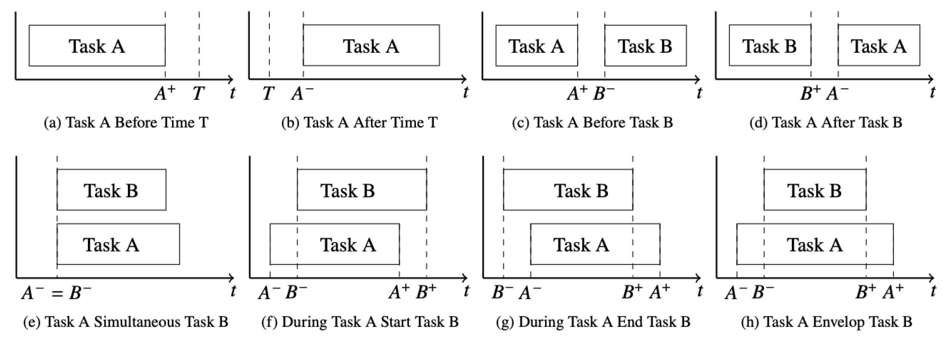
3.1. Temporal Constraints

“Task A Before Time T” and “Task A After Time T” in Table 2 are about one task and a time limitation. “Task A Before Task B” and “Task A Before Task B” are precedence conditions between two tasks. The remaining four constraints are more complicated: “Task A Simultaneous Task B” means that Task A and B should be started simultaneously. “During Task A Start Task B” implies that Task B should be started while performing Task A. “During Task A End Task B” denotes that Task B should be finished while performing Task A. “Task A Envelop Task B” indicates that Task B should be both started and finished while performing Task A. Since one UAV cannot perform two tasks simultaneously, different UAVs should be assigned to perform tasks A and B. Therefore, for these four complicated constraints, the additional constraint ‘ U A V A U A V B ’ needs to be added. U A V A means the UAV performing task A. Algebraic expressions have five types: “A 0 < T”, “A 0 > T”, “A 0 < B 0 ”, “A 0 = B 0 ”, and “ U A V A U A V B ”. A 0 is common form of A + or A . After representing the constraints with algebraic forms, some constraints are induced trivially. For example, if there are constraints ‘ A + < B ’ and ‘ B + < C ’, then ‘ A + < C ’ is natural. If there are constraints ‘ A = B ’ and ‘ B = C ’, then ‘ A = C ’ is reasonable. The rest of the details are presented in Table 3. Generating all the induced constraints enables convenient computation of loitering times and penalty values.

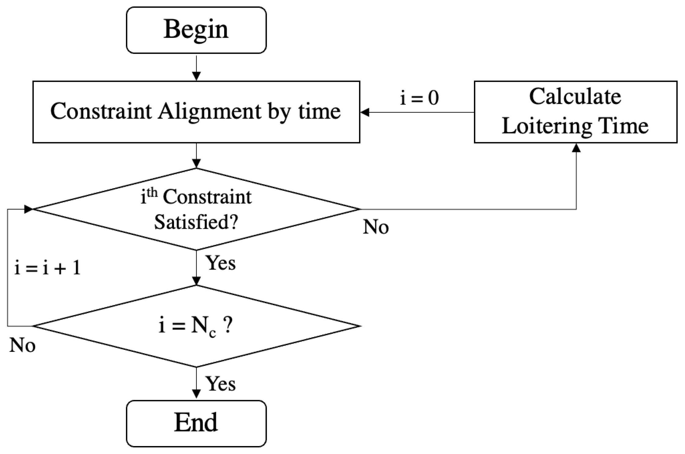
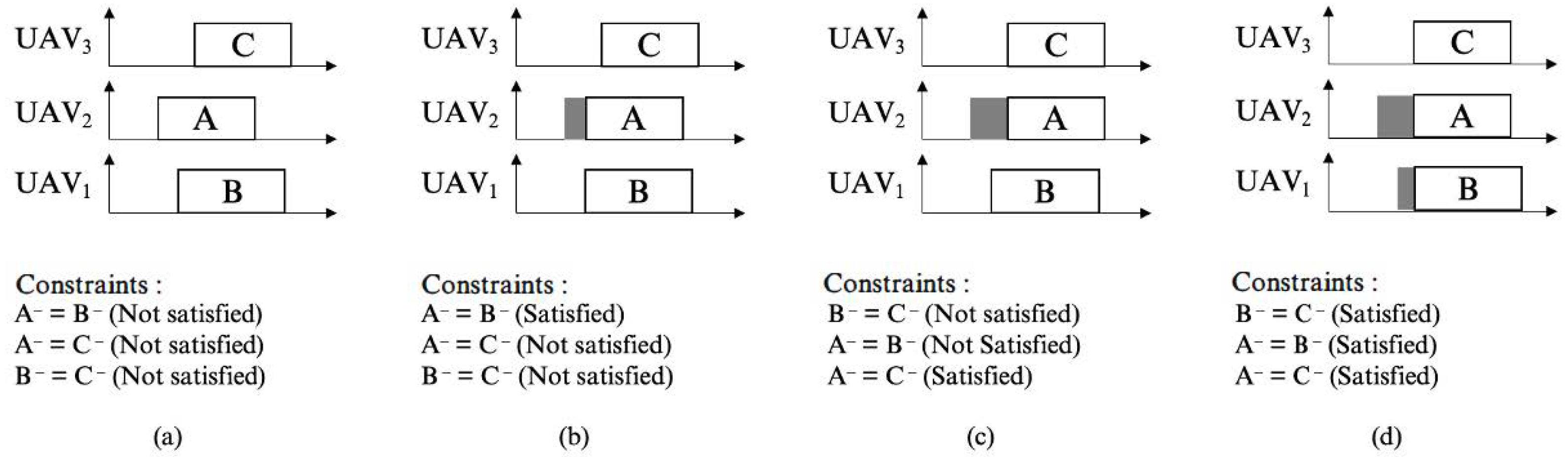
3.2. Loitering Time Calculation Method

To solve the task allocation problem, we define the path ( P ) and loitering time ( W ) in Section 2.2. Temporal constraints can be satisfied with the loitering time ( w i l ). In this chapter, a method is suggested to determine the value of loitering times ( w i l ). This method is inspired by [30]. The loitering time is the waiting time between the arrival to an area to perform a task and the starting time of the task. Before calculation of the loitering time, there are a few precedence conditions, for which constraints are represented with algebraic forms and trivially induced constraints are added. Also, it is necessary to allocate all tasks and to calculate the starting and finishing times for each task. To calculate arrival times to the locations for specific tasks, the distances between the UAVs and tasks and the velocities of the UAVs are used.
The procedure for loitering time calculation is depicted in Figure 2. In simple terms, loitering time is a variable that ensures compliance with all temporal constraints. Adding a loitering time to a particular task also changes the starting times for subsequent tasks that are assigned to the same UAV. Hence, adding a loitering time first to a task with an early starting time is a way to reduce the amount of computation. Therefore, it is necessary that the temporal constraints are sorted in chronological order before calculating a loitering time. In the case of constraints related to two tasks, the reference time is based on the earlier of the starting times of the two tasks associated with the temporal constraints. In the cases of “Task A Before Time T” and “Task A After Time T”, the reference time is the starting time of task A. With reference times, constraints are aligned in chronological order. If constraints are not satisfied, the required loitering time is added to satisfy this. After adding a loitering time to a particular task, the starting and finishing times of tasks that start after that task’s starting time are changed. Hence, constraints are re-aligned with delayed starting times by injecting loitering times. After that, checking the satisfaction is performed from the first of the aligned list of constraints to the end. Loitering time calculations are completed if all conditions are satisfied. For example, when task A initiates before time T under the “Task A After Time T” constraint, a UAV waits at the location of task A without performing the task, allowing it to start later than time T. For simultaneous constraints about task A and B, if a UAV arrives first at the position of task A, it waits for the start of task B. Namely, a loitering time is a waiting time to satisfy temporal constraints.
Figure 3 illustrates a detailed example of the procedures for calculating a loitering time. First, tasks are allocated and constraints are aligned chronologically. After that, a loitering time is calculated sequentially. In Figure 3b, the loitering time (gray) is added for task A, and the constraint ‘ A = B ’ becomes satisfied. Eventually, all constraints are satisfied in Figure 3d after a few iterations of aligning constraints and adding loitering times. The precedence constraints and simultaneous constraints could be satisfied with loitering times. However, as the two constraints ‘ A 0 < T 1 ’ and ‘ U A V A U A V B ’ cannot be satisfied by adding loitering times, they must be satisfied prior to the loitering time calculation. To satisfy these constraints, a penalty value is used. The penalty value is calculated similar to the loitering time.

3.3. Penalty Value Calculation

Generating a feasible path is a prerequisite for calculating the loitering time. To obtain a feasible path, we use a penalty function, and trivially induced constraints are generated in order to calculate the penalty at each step. Without generating these constraints, some tasks may be allocated to infeasible locations. For example, if there are two constraints, ‘ A + < B ’ and ‘ B + < C ’, and only task A among A, B, and C is allocated, task C can be allocated before task A because there are no relationships expressed mathematically. Therefore, penalty values can prevent infeasible allocations with regard to every original and induced constraint.
As mentioned in the previous chapter, the three constraints ‘ A 0 > T 1 ’, ‘ A 0 < B 0 ’, and ‘ A 0 = B 0 ’ can be satisfied by incorporating loitering times, so they have mild penalty values. However, constraints ‘ A 0 < T 1 ’ and ‘ U A V A U A V B ’ cannot be satisfied by adding loitering times. Therefore, the penalty values for these constraints are set to a very large number. The penalty value is calculated for each constraint, and every penalty value is summed. By applying this concept, even if some constraints are not satisfied, it is possible to obtain an initial allocation result that satisfies as many constraints as possible.

4. Modification of Existing Heuristic Algorithms for the Constrained Task Allocation

To solve constrained task allocation problems, a genetic algorithm, simulated annealing, and heuristics are suitable options. Genetic algorithms and simulated annealing are renowned meta-heuristic approaches employed to address problems of diverse types. The goal of an algorithm for constrained task allocation is to calculate the path ( P ) and the loitering time ( W ) while minimizing makespan. To achieve the goal, the genetic algorithm, simulated annealing, and heuristics need to be refined. The genetic algorithm (GA) and simulated annealing (SA) are meta-heuristics; therefore, task allocation methods are newly established. The sequential greedy algorithm (SGA) is a centralized version of the consensus-based bundle algorithm (CBBA) [31]. It is a famous market-based algorithm. It generates a path to maximize the total score obtained by all UAVs. To consider both the makespan and the constraints, SGA should be modified also. All three algorithms utilize the loitering time and penalty calculation techniques to satisfy temporal constraints. The algorithms generate paths, and after path generation, loitering calculations are performed for the three algorithms.

4.1. The Sequential Greedy Algorithm

The SGA is a heuristic-based algorithm, so usually it has a lower computation load than meta-heuristics. SGA’s goal is to minimize the total cost or maximize the total score gained by each UAV. Therefore, the scoring function needs to be changed to handle the makespan. The equation shown below explains the scoring function of the ith UAV’s path ( p i ).
S i p i = l λ T i , l c ¯ i , l
This equation, which originates from [31], calculates the score for p i by summing the score of each task using a discount factor λ that is a positive value smaller than 1. Therefore, tasks performed later receive a lower score. The compatibility value c ¯ i , l is either 1 or 0 depending on whether UAV ith can perform task l or not. T i , l represents the operation time for task l along U A V i ’s path. Due to the discount factor, a higher score is awarded for completing tasks sooner. At each step, the SGA selects the combination of UAV and task that has the highest score. Once a task is allocated to a UAV, a score is calculated that accounts for the increment of the score for the ith UAV’s path and the total penalty value incurred when allocating the task. The maximum value of this summation is determined by inserting the mission into every location on the path. V k ( P j , W ) represents the penalty value for the kth constraint when j is inserted in p i . In the case of total path ( P ), the symbol P j means P contains the task j at some location in P . However, the symbol p i l j means task j is inserted at the lth position in U A V i ’s path. The algorithm iterates N t times until all tasks are allocated. This procedure is depicted in Algorithm  1. Once all tasks are allocated, a loitering time is calculated.
Algorithm 1 Sequential Greedy Algorithm
1:
J a =
2:
P = ( p 1 , p 2 , , p N u ) , W = ( w 1 , w 2 , , w N u )
3:
for  n = 1 to N t  do
4:
    c i j = max l ( S i p i l j S i p i k V k ( P j , W ) ) , i , j I × J
5:
    c i j = 0 , i I , j J a
6:
    i , j = argmax ( i , j ) c i j
7:
    l = argmax l S i p i l j
8:
    p i = p i l j i = i
9:
    J a = J a e n d j
10:
end for

4.2. The Genetic Algorithm

One of the famous meta-heuristic methods is the genetic algorithm. The algorithm consists of chromosome expression and operations for crossover, mutation, and selection [30]. For our scenario, a chromosome has two rows: one is for UAVs and the other is for tasks. A row of UAVs can have duplicate values, which means that UAVs can perform more than one task, and a row of tasks cannot have duplicated values. Hence, the number of columns is the same as the number of tasks. Populations are generated randomly in the initial phase, and parent chromosomes are selected by a roulette wheel selection. After parent selection, a crossover operation is performed as depicted in Figure 4b. Firstly, breaking points for UAVs and tasks are selected, and then offspring take the former part from one parent and take the latter part from the other parent. For a row of tasks, the former part is just transferred from parent to offspring. However, the genes of the latter part are filled with the tasks not assigned to the former part (while avoiding duplication). The order of filling is arithmetic. After crossover, offspring are generated, and three different mutation operations are performed. First, one random gene in the UAV row becomes a different UAV. Second, two random genes in the row of tasks are swapped. Third, two random genes that belong to the same UAV in a row of tasks are swapped. Usually, changing the paths for specific UAVs makes better results. Therefore the third mutation operation in Figure 4(c3) is added. The next generations are selected by higher fitness.
Before the calculation of fitness, a loitering time calculation should be performed to get the makespan. Fitness is defined as shown below:
F i t n e s s = ( max i T i ( p i , w i ) + η i T i ( p i , w i ) + k V k ( P , W ) )
T i ( p i , w i ) is the operation time for U A V i . The second term, η i T i ( p i , w i ) , is a summation of the operation times for every UAV. This term is applied for improving not only the UAV that needs the longest time but also other UAVs’ paths. If η is too big, then the algorithm tries to minimize not the makespan but a summation of the operation time. Therefore, η has a value much smaller than unity. V k ( P , W ) is the penalty value for the kth constraint.

4.3. Simulated Annealing

Simulated annealing is also a well-known meta-heuristic method. Initially, each UAV’s path is generated randomly. After that, random neighbors are selected repeatedly. If a neighbor has a higher score, the neighbor is selected for the current solution. However, with low probability, a neighbor that has a lower score than the current can be chosen. The final solution has the maximized score. The neighbor can be selected with the procedure represented in Figure 5. Firstly, randomly selected elements are removed from the path. Next, the removed elements are allocated random positions in paths. Finally, a specific UAV’s path is shuffled with low probability. There are three termination criteria: a temperature that is sufficiently low, the iteration number exceeding the maximum iterations, and the best value remaining unchanged for several iterations. The equation for fitness is the same as the genetic algorithm. Like the genetic algorithm, a loitering time is calculated after all tasks are allocated.

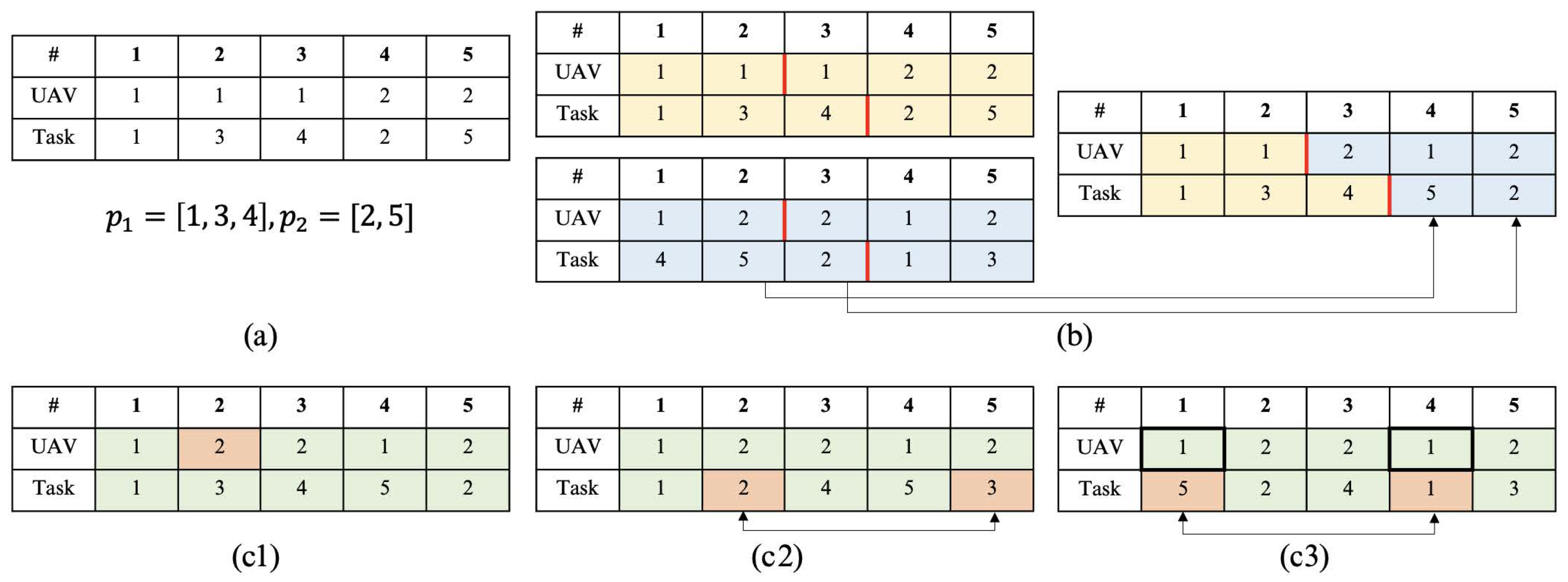
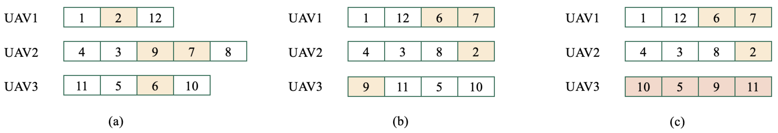
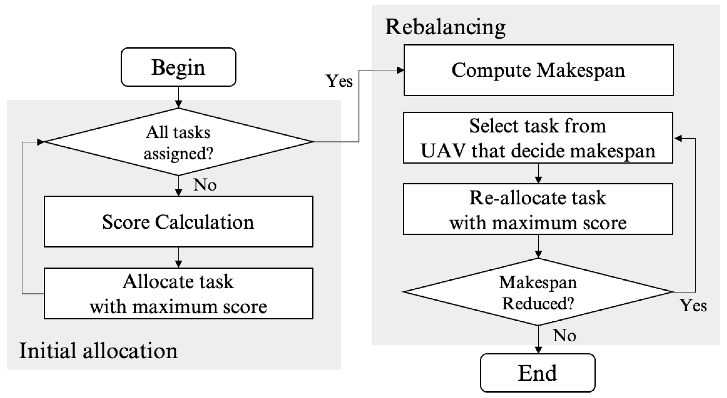
5. The Rebalancing Algorithm

5.1. Algorithm Structure

In this section, we present the proposed rebalancing algorithm. In essence, the initial allocation step involves a greedy procedure for generating the initial path, and the rebalancing step serves as an improvement method for task exchange among UAVs. Before solving the allocation problem, temporal constraints are represented with algebraic forms, and induced constraints are added to calculate the penalty value. In this algorithm, the initial allocation is performed first. The initial allocation is based on a greedy procedure to select the combination of tasks and UAVs that gives the maximum score at the end time.
To enhance the performance of the algorithm, we suggest the “rebalancing” step. For each iteration in the rebalancing step, a loitering time calculation is performed to get the makespan. The detailed procedure is depicted in Figure 6. The left side of the figure represents the initial allocation step, and the right side of the figure represents the rebalancing step.

5.2. The Initial Allocation Step

The initial allocation is based on the greedy algorithm. For each iteration, a task is allocated in some UAV’s path, and iterations are performed until every task is assigned. The score function c i , j , l for every combination of UAV i, task j, and location l in path p i is shown in the fourth row of Algorithm 2. To consider both the makespan and the summation of the time spent performing tasks, fitness S P , W is introduced (Equation (10)). The score function eventually takes the negative of the fitness changes and all penalty values’ summation. As the penalty values for each constraint are summed, even if some of the constraints are not satisfied, it is possible to find a solution that can satisfy the constraints for the loitering time calculation procedure as much as possible. When compatibility c ¯ i , j is zero or task j is already assigned, the score become a negative infinite value. After calculation of scores, the combination of UAVs, tasks, and locations in the paths that has the maximum score is selected, and task j is assigned to location l in UAV i ’s path. Usually, the fitness increases after the allocation of some task, and the fitness value becomes negative. In other words, the algorithm finds a combination that creates a smaller increase in the makespan. Also, the result of task allocation satisfies constraints that have big penalty values after this step, and the other constraints become satisfied after adding loitering time.
S P , W = max i T i ( p i , w i ) + η i T i ( p i , w i )
Algorithm 2 Initial Allocation
1:
J a =
2:
P = ( p 1 , p 2 , , p N u ) , W = ( w 1 , w 2 , , w N u )
3:
for  n = 1 to N t  do
4:
    c i , j , l = S P , W S P j , W k V k ( P j , W ) , i , j I × J , l L p i
5:
    c i , j , l = i n f , i I , j J a , l L p i
6:
   if c ¯ i , j = 0 , then c i , j , l = i n f ,
7:
    i , j , l = argmax ( i , j , l ) c i , j , l
8:
    p i = p i l j i = i
9:
    J a = J a e n d j
10:
end for

5.3. The Rebalancing Step

At the beginning of each iteration in the rebalancing step, the UAV that has the maximum operation time is selected. Then, each task in the UAV’s path is detached and is attached to another location in the same UAV’s path or another UAV’s path. The symbol p i j signifies the detachment of task j from UAV i’s path ( p i ). Unlike the initial allocation, the loitering time is calculated in order to compute scores. The method to calculate the loitering time is represented in Section 3.2. To satisfy temporal constraints, the loitering time is calculated. If the loitering time value of a UAV is too large, then the UAV should remove the task that causes the large loitering time, and that task is added to another UAV. The score is the decrease in fitness. If the fitness is increased, then it is a worse path and the score should be zero. When the summation of penalty values becomes larger than zero, the score is set to be zero. If all penalty values are zero with a proper initial allocation and loitering time calculation, then the score also becomes zero. When compatibility c ¯ i , j is zero, the score becomes zero. There are many conditions for having a zero score. Hence, a re-allocation should be performed if the maximum score is non-zero. This procedure is iterated until the maximum score becomes zero. As the path is only changed when the fitness decreases, the rebalancing step can be seen as a descent method for fitness from an optimization perspective. This procedure is depicted in Algorithm 3.
Algorithm 3 Rebalancing
1:
P = ( p 1 , p 2 , , p N u ) , W = ( w 1 , w 2 , , w N u )
2:
for  n = 1 to N t  do
3:
    i l = argmax i T i ( p i , w i )
4:
    P = ( , p i l j , , p i l j , ) , W = ( , w i l w i l j , , w i l w i l , ) , i I , j p i l , l L p i
5:
    W = C a l L o i t e r i n g ( )
6:
    c i , j , l = S P , W S P , W , i I , j p i l , l L p i
7:
    c i , j , l = 0 , j p i l
8:
   if S P , W > S P , W o r k V k ( P , W ) > 0 o r c ¯ i , j = 0 , then c i , j , l = 0
9:
    v a l = max ( i , j , l ) c i , j , l
10:
   if  v a l > 0  then
11:
      i , j , l = argmax ( i , j , l ) c i , j , l
12:
      p i = p i l j
13:
      p i = p i , i i
14:
   else
15:
     break;
16:
   end if
17:
end for

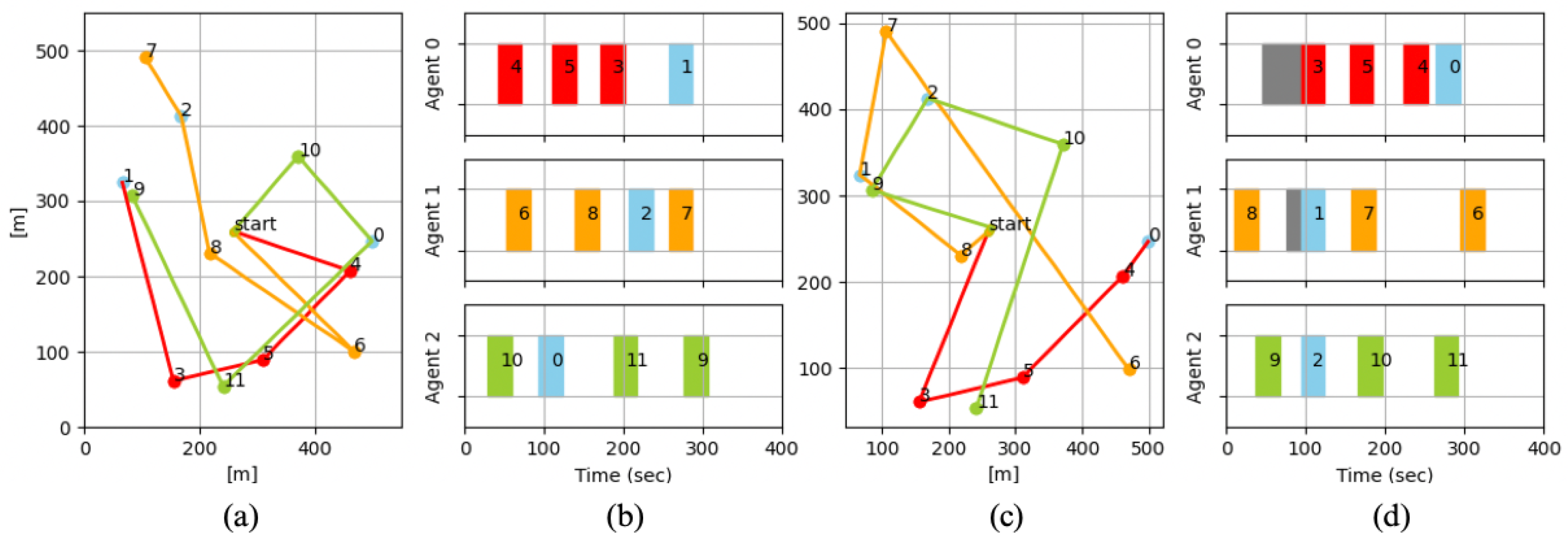
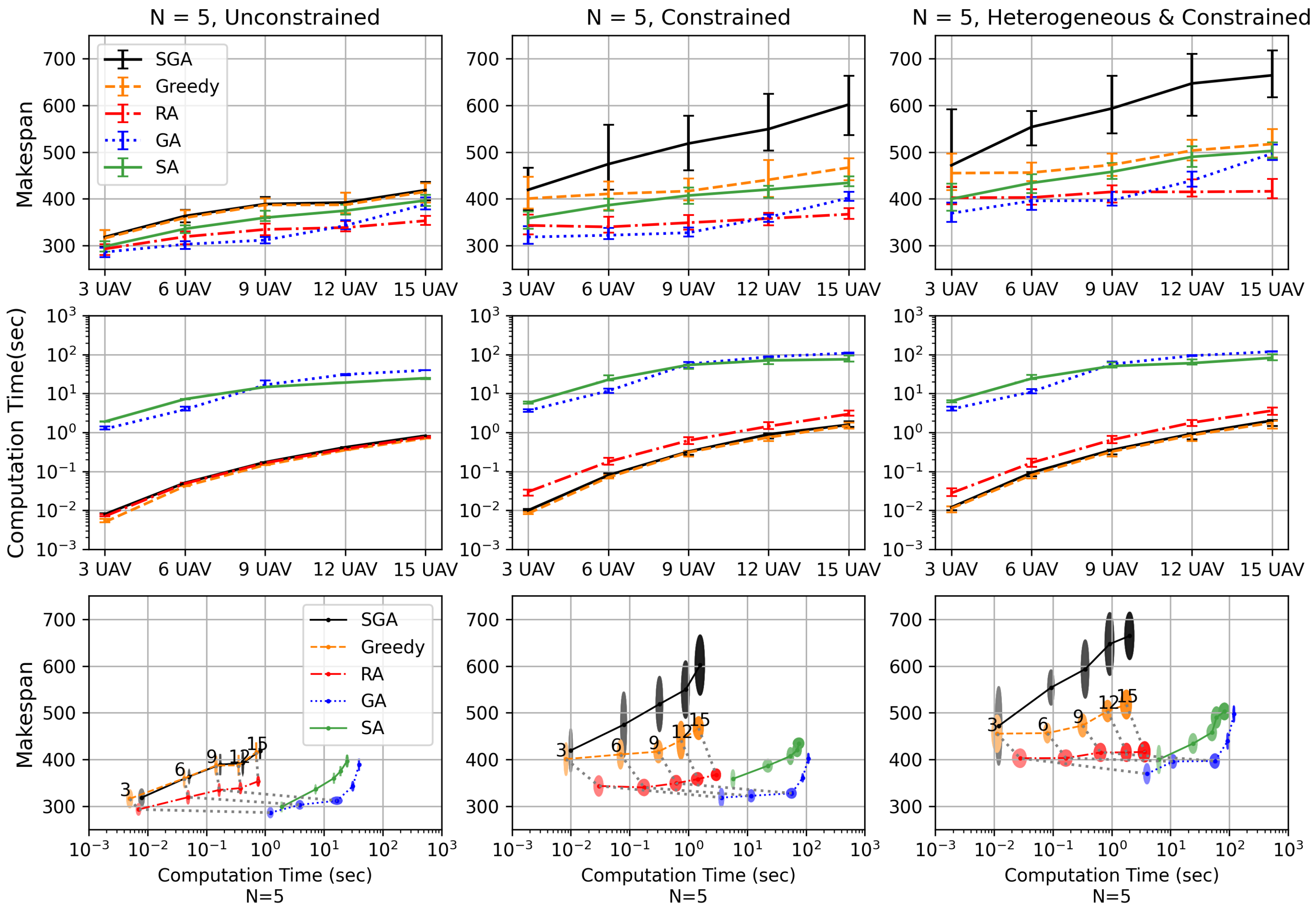
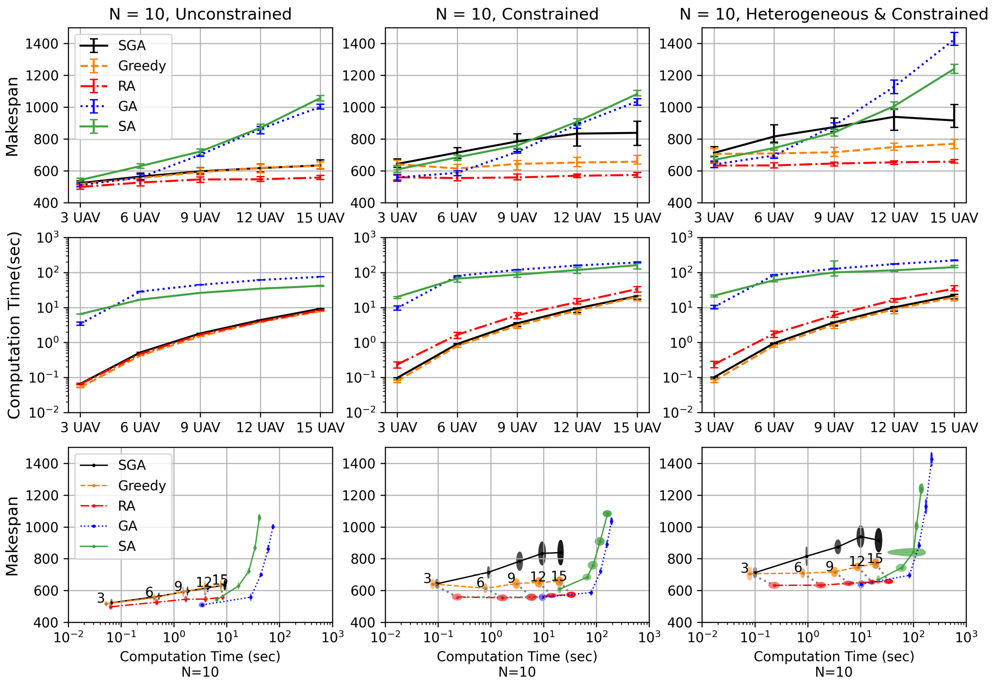
6. Numerical Simulation

We compared the performance and computation time of the rebalancing algorithm and other algorithms. If the tasks are evenly distributed within the area, every UAV’s path will have an equal number of tasks. Hence, we defined new variable N = N t / N u . It is the number that represents the number of tasks divided by the number of UAVs. We performed simulations for cases of N = 5 , 10 . Also, the number of UAVs varies from 3 to 15 for each value of N. Depending on the number of tasks, the area where the task takes place is assumed to grow as the ratio between the area and N t is maintained. If the mission area remains the same and only the number of tasks increases, the gap between tasks is narrowed, and it would be hard to figure out why the entire task termination time would be reduced: i.e., due to the algorithm’s performance or the reduced gap. Therefore the tasks are in a square area for which one side’s length is 0.3 km × (number of UAVs) 0.5 to maintain the ratio between the number of tasks and the mission area. Initially, UAVs are located in a circle with a radius of 5 m at the center of the square, the duration of all tasks is 30 s, and the speed of UAVs is defined at 5 m/s. Also, there are three cases: unconstrained condition and constrained condition with homogeneous system and constrained condition with heterogeneous system. For heterogeneous systems, there are three types of UAVs and four types of tasks, as in Figure 7. The light-blue-colored task is a common task that can be done by any UAV, and other colors can be done by a same-colored UAV. Both the UAVs and tasks have almost the same number for each type. If N = 5 , N u = 12 , and N t = 60 , there would be four red-colored UAVs and fifteen red-colored missions. If the number cannot be divided evenly, the number of UAVs of each color may vary slightly. When N is equal to 5 or 10, a total of six conditions can be obtained by applying three conditions to each value of N. Figure 7 describes the distribution of UAVs and tasks and a temporal sequence for each UAV. The constraints are “Task 1, 2, 3 should be started simultaneously” and “Task 0 should be after Task 1, 2, 3”. The gray area means a loitering time: the time from arrival to starting the task. The line in Figure 7a,c means the UAV’s path. The color represents the UAV and task type. UAV0 is red, UAV1 is orange, and UAV2 is green. Each UAV can perform the same-colored tasks and light-blue-colored tasks. As represented in Figure 7, every algorithm can consider both the heterogeneous system and temporal constraints. If not, the makespan would be very large. When the constraints are violated, loitering time is added over and over again until the algorithm is forced to stop, and if the tasks are allocated without consideration of compatibility, it takes a very long time to perform tasks.
In the genetic algorithm, the total number of chromosomes in each generation is 80, and 40 offspring are generated through crossover and mutation operations. After the operations, 80 chromosomes are selected based on their fitness score from the prior generation and new offspring. The mutation probabilities for the first, second, and third mutation operations are 1%, 1%, and 5%, respectively. The maximum number of iterations is set to 4000. However, if the same fitness score is maintained for 500 consecutive iterations, the iteration is stopped.
For the simulated annealing algorithm, elements are selected with a 5% probability and are removed, and the removed elements are allocated to a random position. Additionally, a randomly selected UAV’s path is shuffled with a 5% probability.
Figure 8 represents the results of numerical simulation. To get the averages and variances, 50 runs are performed for each case. The upper side of the figure is a comparison of the makespan, the middle side of the figure is a comparison of the computation time, and the lower side of the figure is a comparison of both the makespan and computation time. For the upper side and the middle side, 25th and 75th percentiles are represented with bars. For the lower side, an ellipse is used to show two variables’ variance. The horizontal diameter of the ellipse is the 25th and 75th percentiles of the computation time, and the vertical diameter of the ellipse is the 25th and 75th percentiles of the makespan. The abbreviation “SGA” means the sequential greedy algorithm, “Greedy” means the initial allocation phase of the proposed algorithm, “RA” is the rebalancing algorithm, and “GA” and “SA” mean genetic algorithm and simulated annealing, respectively. Usually, the makespan increases along with the number of UAVs, and the makespan when constrained is longer than for the no-constraint condition.
Usually, the more complicated the problem, the longer the calculation time. As depicted in Figure 8 and Figure 9, the heterogeneous and constrained conditions need longer makespans than other conditions. Meta-heuristics need a much longer computation time than heuristics. The rebalancing algorithm needs almost the same computation time with only the initial allocation step (greedy) and SGA for unconstrained conditions. However, it needs more computation to calculate loitering times for the rebalancing step when constraints are applied. Still, its calculation time is much lower than that of meta-heuristics. The genetic algorithm shows the best performance when N = 5 and there are fewer than nine UAVs. However, about 100 times more time is needed compared to RA. As the size of the problem increases, the performance of the genetic algorithm and simulated annealing decreases, resulting in a significant increase in makespan. If N is constant, the number of tasks taken by one UAV is constant regardless of the number of UAVs when the assignment is well done. And the mission area is widened according to the number of tasks, so the distance between missions becomes similar, so makespan should also be constant. At N = 10 for the heterogeneous and constrained conditions, the average makespan of the RA is 632 s for 3 UAVs, and it become 657 s for 15 UAVs. This is only a 4% increase. Therefore, it can be seen that the RA is working well.
The goal of these algorithms is to minimize the makespan, which is expected to be the same for any number of UAVs when the task density is constant. The rebalancing algorithm shows promising results, as it has an almost equal makespan when the number of UAVs is increased. In unconstrained conditions, SGA and only the initial allocation step (greedy) have similar makespans. However, only the initial allocation step (greedy) has better performance than SGA for constrained conditions. And adding a rebalancing step can reduce the makespan. When N u , N t is small, the genetic algorithm has a much shorter makespan than others. However, only the initial allocation step (greedy) and the rebalancing algorithm compose a Pareto front for cases other than N = 5 and N u < 12 or N = 10 and N u < 6 . This represents that the meta-heuristic algorithm is not suitable for large-scale problems. It already needs a lot of computation to improve performance, but the computation loads become much larger.
The rebalancing algorithm requires more computational resources than simpler algorithms like SGA and greedy, but it can generate paths that have shorter makespans. In particular, the algorithm is more effective in constrained conditions, where the improvements to solution quality are more significant compared to those of unconstrained conditions. This is because the rebalancing algorithm is designed to consider both the constraints and the heterogeneity of the system, making it suitable for complex problems in real-world scenarios. As a result, the rebalancing algorithm is a promising approach for solving task allocation problems that involve multiple constraints and heterogeneous multi-UAV systems.

7. Conclusions

This paper presents a novel variable called “loitering” and a multi-UAV mission planning technique based on a heuristic algorithm that addresses task allocation problems in heterogeneous systems with various temporal constraints. This algorithm is performed by a centralized planner, so it is appropriate for generating initial paths for every UAV. The proposed technique calculates the loitering time to enable efficient planning that satisfies the temporal constraints while minimizing the makespan. The proposed approach is compared with three algorithms: the genetic algorithm (GA), simulated annealing (SA), and the sequential greedy algorithm (SGA). The numerical simulation results show that the rebalancing algorithm outperforms the SGA while requiring only a slightly longer computation time. Moreover, the rebalancing algorithm overwhelms the GA when the number of UAVs and tasks becomes large, in which case the meta-heuristic algorithms may struggle to generate accurate solutions. Therefore, the rebalancing algorithm is more appropriate for general cases. Additionally, the initial allocation step can create a path with a shorter makespan than that of SGA, and the makespan becomes much smaller after the rebalancing step in constrained conditions. Overall, the proposed loitering-based approach and the rebalancing algorithm demonstrate promising results for solving multi-UAV mission planning problems in heterogeneous systems with various temporal constraints. Future research directions are expected to expand on several fronts. One of the directions is to consider UAV endurance. Certainly, considering the inherent limitations of UAV endurance is crucial for developing realistic algorithms. The need for periodic resupply due to limited flight endurance can be viewed as a constraint for which the UAV must visit a replenishment base after a specific duration of flight. In future research, incorporating such considerations into algorithmic frameworks would contribute to the development of more practical and realistic solutions. Addressing the challenge of optimizing routes and scheduling visits to resupply bases in response to UAV endurance limitations is a promising avenue for enhancing the realism and applicability of the algorithms in UAV operations.

Author Contributions

Conceptualization, N.-E.H. and J.-W.K.; methodology, B.-M.J.; software, B.-M.J. and Y.-S.O.; validation, D.-S.J. and H.-L.C.; formal analysis, B.-M.J.; data curation, Y.-S.O.; writing—original draft preparation, B.-M.J. and Y.-S.O.; writing—review and editing, D.-S.J., N.-E.H., J.-W.K. and H.-L.C.; visualization, Y.-S.O.; funding acquisition, H.-L.C. All authors have read and agreed to the published version of the manuscript.

Funding

This work was supported by a Korea Research Institute for Defense Technology (KRIT) planning and advancement grant funded by the Korean government (DAPA (Defense Acquisition Program Administration)) (No. KRIT-CT-21-009, Development of Realtime Automatic Mission Execution and Correction Technology based on Battlefield Information, 2021).

Data Availability Statement

Data are contained within the article.

Conflicts of Interest

Authors Nam-Eung Hwang and Joon-won Kim were employed by the company Hanwha Systems Co. The remaining authors declare that the research was conducted in the absence of any commercial or financial relationships that could be construed as a potential conflict of interest.

References

  1. Athanasiadi, N.I.; Mitkas, P.A. An agent-based intelligent environmental monitoring system. Manag. Environ. Qual. Int. J. 2004, 15, 238–249. [Google Scholar] [CrossRef]
  2. Erdelj, M.; Król, M.; Natalizio, E. Wireless sensor networks and multi-UAV systems for natural disaster management. Comput. Netw. 2017, 124, 72–86. [Google Scholar] [CrossRef]
  3. Skobelev, P.; Budaev, D.; Gusev, N.; Voschuk, G. Designing Multi-agent Swarm of UAV for Precise Agriculture. In Highlights of Practical Applications of Agents, Multi-Agent Systems, and Complexity: The PAAMS Collection, Proceedings of the International Workshops of PAAMS 2018, Toledo, Spain, 20–22 June 2018; Springer: Cham, Switzerland, 2018; pp. 47–59. [Google Scholar] [CrossRef]
  4. Shehory, O.; Kraus, S. Methods for task allocation via agent coalition formation. Artif. Intell. 1998, 101, 165–200. [Google Scholar] [CrossRef]
  5. Notomista, G.; Mayya, S.; Hutchinson, S.; Egerstedt, M. An optimal task allocation strategy for heterogeneous multi-robot systems. In Proceedings of the 2019 18th European Control Conference (ECC), Naples, Italy, 25–28 June 2019; pp. 2071–2076. [Google Scholar] [CrossRef]
  6. Johnson, L.; Ponda, S.; Choi, H.L.; How, J.P. Asynchronous decentralized task allocation for dynamic environments. Infotech Aerosp. 2011, 2011, 1441. [Google Scholar] [CrossRef]
  7. Whitten, A.K.; Choi, H.L.; Johnson, L.B.; How, J.P. Decentralized task allocation with coupled constraints in complex missions. In Proceedings of the 2011 American Control Conference, San Francisco, CA, USA, 29 June–1 July 2011; pp. 1642–1649. [Google Scholar] [CrossRef]
  8. Choi, H.L.; Whitten, A.K.; How, J.P. Decentralized task allocation for heterogeneous teams with cooperation constraints. In Proceedings of the 2010 American Control Conference, Baltimore, MD, USA, 30 June–2 July 2010; pp. 3057–3062. [Google Scholar] [CrossRef]
  9. Garcia, E.; Casbeer, D.W. Cooperative task allocation for unmanned vehicles with communication delays and conflict resolution. J. Aerosp. Inf. Syst. 2016, 13, 1–13. [Google Scholar] [CrossRef]
  10. Kim, K.S.; Kim, H.Y.; Choi, H.L. Minimizing communications in decentralized greedy task allocation. J. Aerosp. Inf. Syst. 2019, 16, 340–345. [Google Scholar] [CrossRef]
  11. Pendharkar, P.C. An ant colony optimization heuristic for constrained task allocation problem. J. Comput. Sci. 2015, 7, 37–47. [Google Scholar] [CrossRef]
  12. Chen, G.; Cruz, J.B. Genetic algorithm for task allocation in UAV cooperative control. In Proceedings of the AIAA Guidance, Navigation, and Control Conference and Exhibit, Austin, TX, USA, 11–14 August 2003; p. 5582. [Google Scholar] [CrossRef]
  13. Liu, C.; Kroll, A. A centralized multi-robot task allocation for industrial plant inspection by using a* and genetic algorithms. In Artificial Intelligence and Soft Computing, Proceedings of the 11th International Conference, ICAISC 2012, Zakopane, Poland, 29 April–3 May 2012; Proceedings, Part II 11; Springer: Berlin/Heidelberg, Germany, 2012; pp. 466–474. [Google Scholar] [CrossRef]
  14. Wang, Z.; Liu, L.; Long, T.; Wen, Y. Multi-UAV reconnaissance task allocation for heterogeneous targets using an opposition-based genetic algorithm with double-chromosome encoding. Chin. J. Aeronaut. 2018, 31, 339–350. [Google Scholar] [CrossRef]
  15. Page, J.A.; Keane, T.M.; Naughton, T.J. Multi-heuristic dynamic task allocation using genetic algorithms in a heterogeneous distributed system. J. Parallel Distrib. Comput. 2010, 70, 758–766. [Google Scholar] [CrossRef] [PubMed]
  16. Page, J.A.; Keane, T.M.; Naughton, T.J. Genetic algorithm-based task allocation in multiple modes of human–robot collaboration systems with two cobots. Int. J. Adv. Manuf. Technol. 2022, 119, 7291–7309. [Google Scholar] [CrossRef]
  17. Chen, J.; Yang, Y.; Wu, Y. Multi-robot task allocation based on robotic utility value and genetic algorithm. In Proceedings of the 2009 IEEE International Conference on Intelligent Computing and Intelligent Systems, Shanghai, China, 20–22 November 2009; Volume 2, pp. 256–260. [Google Scholar] [CrossRef]
  18. Rauniyar, A.; Muhuri, P.K. Multi-robot coalition formation problem: Task allocation with adaptive immigrants based genetic algorithms. In Proceedings of the 2016 IEEE International Conference on Systems, Man, and Cybernetics (SMC), Budapest, Hungary, 9–12 October 2016; pp. 137–142. [Google Scholar] [CrossRef]
  19. Sujit, P.; George, J.; Beard, R. Multiple UAV task allocation using particle swarm optimization. In Proceedings of the AIAA Guidance, Navigation and Control Conference and Exhibit, Honolulu, HI, USA, 18–21 August 2008; p. 6837. [Google Scholar] [CrossRef]
  20. Attiya, G.; Hamam, Y. Task allocation for maximizing reliability of distributed systems: A simulated annealing approach. J. Parallel Distrib. Comput. 2006, 66, 1259–1266. [Google Scholar] [CrossRef]
  21. Mosteo, A.R.; Montano, L. Simulated annealing for multi-robot hierarchical task allocation with flexible constraints and objective functions. In Proceedings of the Workshop on Network Robot Systems: Toward Intelligent Robotic Systems Integrated with Environments, Beijing, China, 9–15 October 2006. [Google Scholar]
  22. Beck, J.E.; Siewiorek, D.P. Simulated annealing applied to multicomputer task allocation and processor specification. In Proceedings of the SPDP’96: 8th IEEE Symposium on Parallel and Distributed Processing, New Orleans, LA, USA, 23–26 October 1996; pp. 232–239. [Google Scholar] [CrossRef]
  23. Kashani, M.H.; Jahanshahi, M. Using simulated annealing for task scheduling in distributed systems. In Proceedings of the 2009 International Conference on Computational Intelligence, Modelling and Simulation, Brno, Czech Republic, 7–9 September 2009; pp. 265–269. [Google Scholar] [CrossRef]
  24. DiNatale, M.; Stankovic, J.A. Applicability of simulated annealing methods to real-time scheduling and jitter control. In Proceedings of the 16th IEEE Real-Time Systems Symposium, Pisa, Italy, 5–7 December 1995; pp. 190–199. [Google Scholar] [CrossRef]
  25. Godoy, J.; Gini, M. Task allocation for spatially and temporally distributed tasks. In Intelligent Autonomous Systems, Proceedings of the 12th International Conference IAS-12, Jeju Island, Republic of Korea, 26–29 June 2012; Springer: Berlin/Heidelberg, Germany, 2013; pp. 603–612. [Google Scholar] [CrossRef]
  26. Amador, S.; Okamoto, S.; Zivan, R. Dynamic multi-agent task allocation with spatial and temporal constraints. In Proceedings of the AAAI Conference on Artificial Intelligence, Quebec City, QC, Canada, 27–31 July 2014; Volume 28, pp. 1384–1390. [Google Scholar] [CrossRef]
  27. Mitiche, H.; Boughaci, D.; Gini, M. Iterated local search for time-extended multi-robot task allocation with spatio-temporal and capacity constraints. J. Intell. Syst. 2019, 28, 347–360. [Google Scholar] [CrossRef]
  28. Zhao, X.; Zong, Q.; Tian, B.; Zhang, B.; You, M. Fast task allocation for heterogeneous unmanned aerial vehicles through reinforcement learning. Aerosp. Sci. Technol. 2019, 92, 588–594. [Google Scholar] [CrossRef]
  29. Schwalb, E.; Vila, L. Temporal constraints: A survey. Constraints 1998, 3, 129–149. [Google Scholar] [CrossRef]
  30. Jeong, B.M.; Jang, D.S.; Hwang, N.E.; Kim, J.W.; Choi, H.L. Genetic algorithm based multi-UAV mission planning method considering temporal constraints. J. Aerosp. Syst. Eng. 2023. [Google Scholar]
  31. Choi, H.L.; Brunet, L.; How, J.P. Consensus-based decentralized auctions for robust task allocation. IEEE Trans. Robot. 2009, 25, 912–926. [Google Scholar] [CrossRef]
Figure 1. Graphical illustration of temporal constraints.
Aerospace 10 01032 g001
Figure 2. Loitering time calculation.
Aerospace 10 01032 g002
Figure 3. The description of loitering time calculation procedure. The box with an alphabet represent a start and an end of the task, The gray shadow represent a loitering time before performing a task.
Aerospace 10 01032 g003
Figure 4. Genetic algorithm for task allocation: (a) graphical illustration of chromosome, (b) crossover operation, and (c1c3) 3 different types of mutation operations.
Aerospace 10 01032 g004
Figure 5. The neighbor search procedure in simulated annealing for task allocation: (a) randomly selected elements, (b) re-allocated elements, and (c) shuffled sequence.
Aerospace 10 01032 g005
Figure 6. The structure of the rebalancing algorithm.
Aerospace 10 01032 g006
Figure 7. Heterogeneous task allocation example—UAV 3, Task 12: (a,b) unconstrained task allocation example and (c,d) constrained task allocation example. The task numbers 0 11 in (a,c) represent each task’s position and the task numbers in (b,d) show a period to perform each task.
Aerospace 10 01032 g007
Figure 8. Simulation results—N ( N U A V / N t a s k ) = 5. The number in the lowest graph represents the agent number, the horizontal length of each ellipse represents the variance of the calculation time, and the vertical length represents the variance of the makespan.
Aerospace 10 01032 g008
Figure 9. Simulation results—N ( N U A V / N t a s k ) = 10. The number in the lowest graph represents the agent number, the horizontal length of each ellipse represents the variance of the calculation time, and the vertical length represents the variance of the makespan.
Aerospace 10 01032 g009
Table 1. Example of compatibility matrix.
UAVCameraThermalLIDAR
Task
Search010
Fixed surv.110
Moving surv.110
Mapping001
Table 2. Algebraic representation of temporal constraints.
#Temporal ConstraintAlgebraic Representation
1Task A Before Time T A + < T
2Task A After Time T A > T
3Task A Before Task B A + < B
4Task A After Task B A > B +
5Task A Simultaneous Task B A = B
6During Task A Start Task B A < B B < A +
7During Task A End Task B A < B + B + < A +
8Task A Envelop Task B A < B B + < A +
Table 3. How to generate induced constraints.
Constraint 1Constraint 2Action
A 0 < T 1 A 0 < T 2 Remove “ A 0 < T 1 ” (if T 1 < T 2 )
Remove “ A 0 < T 2 ” (if T 1 > T 2 )
A 0 > T 2 Infeasible (if T 1 T 2 )
No action (if T 1 > T 2 )
A 0 > B 0 Add “ B 0 < T 1
A 0 < B 0 No action
A 0 = B 0 Add “ B 0 < T 1
A 0 > T 1 A 0 > T 2 Remove “ A 0 > T 2 ” (if T 1 < T 2 )
Remove “ A 0 > T 1 ” (if T 1 > T 2 )
A 0 > B 0 No action
A 0 < B 0 Add “ B 0 > T 1
A 0 = B 0 Add “ B 0 > T 1
A 0 > B 0 A 0 < C 0 Add “ B 0 < C 0
C 0 < A 0 No action
A 0 = B 0 Infeasible
A 0 = C 0 Add “ B 0 < C 0
A 0 = B 0 A 0 = C 0 Add “ B 0 = C 0
Table 4. Penalty calculation.
k th Constraint V k ( P , W )
A 0 < T 1 big number (if violated)
0 (if not)
A 0 > T 1 max( T 1 T A 0 , 0 )
A 0 < B 0 max( T A 0 T B 0 , 0 )
A 0 = B 0 a b s ( T A 0 T B 0 )
U A V A U A V B big number (if violated)
0 (if not)
Disclaimer/Publisher’s Note: The statements, opinions and data contained in all publications are solely those of the individual author(s) and contributor(s) and not of MDPI and/or the editor(s). MDPI and/or the editor(s) disclaim responsibility for any injury to people or property resulting from any ideas, methods, instructions or products referred to in the content.

