Convex Optimization-Based Techniques for Trajectory Design and Control of Nonlinear Systems with Polytopic Range

Abstract

This paper presents new techniques for the trajectory design and control of nonlinear dynamical systems. The technique uses a convex polytope to bound the range of the nonlinear function and associates with each vertex an auxiliary linear system. Provided controls associated with the linear systems can be generated to satisfy an ordering constraint, the nonlinear control is computable by the interpolation of controls obtained by convex optimization. This theoretical result leads to two numerical approaches for solving the nonlinear constrained problem: one requires solving a single convex optimization problem and the other requires solving a sequence of convex optimization problems. The approaches are applied to two practical problems in aerospace engineering: a constrained relative orbital motion problem and an attitude control problem. The solve times for both problems and approaches are on the order of seconds. It is concluded that these techniques are rigorous and of practical use in solving nonlinear trajectory design and control problems.

1. Introduction

This paper presents new techniques for the trajectory design and control of nonlinear dynamical systems. Assuming that the state and control are constrained to convex sets, a sufficient condition for the nonlinear control to be computable by interpolation of controls obtained by convex optimization is stated and proved. This theoretical result leads to two numerical approaches for solving the nonlinear constrained problem: one requires solving a single convex optimization problem and the other requires solving a sequence of convex optimization problems.

The approaches are applied to two spacecraft trajectory design and control problems: (1) a spacecraft is constrained to stay a certain distance from another space object in orbit while moving from one location to another in a finite time; (2) a spacecraft is to change its attitude in a finite time. The first problem may arise in the inspection phase of an on-orbit servicing (OOS) mission [1]. For such a mission, the controlled spacecraft must stay far enough from the target space object for safety reasons but also close enough to efficiently perform the inspection. In general, OOS missions are needed to either repair a damaged spacecraft or to extend the active lifetime of a spacecraft. An example of a spacecraft that has had multiple OOS missions to service it is the Hubble Space Telescope [2]. Beyond OOS missions, there are other types of missions where this type of problem could arise, such as asteroid proximity operations [3,4].

The finite-time attitude control problem arises in optical applications where a picture of a space object is to be taken at a certain time [5]. There may, for example, be a short time window when the lighting of a space object is sufficient due to the relative positions of the space object, the controlled spacecraft, and the sun [6,7]. The problem could also arise when a spacecraft wants to perform an impulsive or so-called ’delta-v’ maneuver [8] and its thrusters need to be oriented in the correct direction.

The class of problems studied in this paper has nonlinear dynamics, and there is a large body of literature on feedback control, optimization, and trajectory design for such systems. The next two subsections situate the present work relative to control-related work and optimization/trajectory-design-related work.

1.1. Control Theory

There are multiple techniques to solve nonlinear control problems based on linearization. One of the most common techniques is feedback linearization [9]. This technique, when applicable, allows one to use well-studied linear control techniques on the linearized problem. Feedback linearization is an exact linearization technique because no approximations are needed. However, errors in state estimation, modeling, and time delays may destabilize the system. Because the nonlinear term is part of feedback, incorporation of control constraints is challenging.

There are other techniques that produce exact linearizations, such as the ones discussed in [10,11]. In both of these cases, a linear system is achieved by the transformation of variables. The challenge is that these types of exact linearizations exist for only a small subset of dynamical systems, and even when they do, the transformation may not be obvious, requiring the control engineer to spend significant time deriving it.

In addition to exact linearization techniques, there are techniques that approximate the nonlinear system by a linear one. The most well-known one is where the Jacobian is evaluated at an operating point. Some of the other techniques include approximation of the Koopman operator and the use of machine learning [12,13,14]. These techniques approximate the nonlinear dynamics by introducing new state variables/lifting functions to arrive at a high-order linear model. The results of this paper leverage ‘auxiliary’ linear systems associated with a nonlinear system; however, neither exact nor approximate linearizations are used.

Yet another technique to linearize a nonlinear system is to use linear parameter-varying (LPV) system [15]. LPV systems have been used to represent nonlinear systems in many applications, such as aerospace, ground vehicle, and robotic control [16]. The controller design for LPV systems usually takes advantage of linear matrix inequalities (LMI) and convex combinations of linear systems [17]. LPV controller techniques are often used in robust control where the model has uncertainty and the controller is designed to be robust for these uncertainties. The LPV controller techniques using LMIs are limited to controllers with asymptotic stability, whereas the controller design technique introduced in this paper can be used to solve fixed finite-time problems. A non-LPV technique where the nonlinear system is bounded by linear ones was introduced in [18].

Control design using control Lyapunov functions has been performed for nonlinear control affine systems with ball-type control constraints [19] and polytopic control constraints [20]. In [20], their algorithm minimizes the control magnitude pointwise in time; as such, it requires the solution of a quadratic program (QP) pointwise in time. Similarly, control barrier functions have been used to simultaneously ensure system ‘safety’ and stability, again often requiring pointwise optimization [21]. The technique in this paper requires the solution of only one SOCP, and then the nonlinear control may be interpolated.

1.2. Optimization and Trajectory Design

Classical approaches for control of linear and nonlinear systems do not account for state and control constraints. When such constraints are present, optimization-based techniques may be used. Most relevant here are the recent results in lossless convexification and sequential convex programming. The fundamental idea in lossless convexification is to relax non-convex constraints to convex form and then prove the relaxation did not introduce new optimal solutions [22]. Motivating this research has been minimum-fuel-type optimal control problems with linear dynamics and annular control constraints [23]. The earliest papers required a technical assumption related to the transversality condition of optimal control. This assumption has recently been weakened, allowing a broader class of problems including ones with fixed final time [24]. The theory has also been extended to problems with linear state constraints [25,26], quadratic state constraints [27,28], and disconnected control sets [29]. For problems with state constraints, a key condition in the proofs is related to the strong observability property of the dynamical system [30].

The theory has also been extended to annularly constrained problems with nonlinear dynamics [31]. The relaxation applies only to the control constraint. Consequently, the relaxed problem remains non-convex because of the nonlinear dynamics and non-convex techniques, such as sequential quadratic programming and sequential convex programming [32,33,34,35], are required to solve the problem. Those techniques rely upon local linearizations/convexifications and iterative updates to converge to local extrema. In sequential convex programming, multiple convex programs must be solved in the process. In contrast, our Theorem 1 provides sufficient conditions for the nonlinear trajectory design and control problem to be solved with a single convex program.

1.3. Contributions

The problem of interest in this paper is a nonlinear control problem with convex state and control constraints. The primary theoretical contribution is a set of sufficient conditions under which the problem is solvable as a single convex program. This is in contrast to:

• Classical control techniques, which do not account for state and control constraints;
• Lossless convexifications, which do not generate convex problems when nonlinear dynamics are present;
• Sequential convex programming, which requires the solution of many convex programs.

Our technique uses a convex polytope to bound the range of the nonlinear function, and associates with each vertex of the polytope an ‘auxiliary’ linear system. The sufficient conditions presented in Theorem 1 guarantee that a feasible control for the nonlinear system is interpolatable from the ‘auxiliary’ linear controls obtained via convex optimization. A conceptual understanding of the proof leads to a ‘resetting approach’ that applies even when the sufficient conditions are violated.

The primary applied contribution is the application of the theory and algorithms to two problems in aerospace engineering. The first problem is a spherically constrained relative orbital motion problem, which has been studied from the lossless convexification [28] and nonlinear dynamics [36] perspectives. The second problem is an attitude control problem using the dynamics of the Euler axis.

1.4. Outline

The remainder of the paper is structured as follows: Section 2 describes the problem of interest, which is a nonlinear control problem with convex state and control constraints, and proves sufficient conditions (see Theorem 1) for the problem to be solvable in a single convex program. A sequential or resetting approach is then outlined for cases in which the sufficient conditions are not satisfied. The theoretical results and associated algorithms are applied to a constrained relative orbital motion problem in Section 3 and an attitude control problem in Section 4. Conclusions are presented in Section 5. Because the paper focuses on discrete-time systems, a particular strategy for discretizing continuous-time systems is presented in Appendix A.

2. Problem and Main Result

This section describes the problem of interest, provides a sufficient condition for its solution as a single convex program, and describes a practical algorithm for implementing the theoretical results. Consider a nonlinear system of the form

$$\dot{x}=Ax+Bu+E\eta \left(x\right),x_0=x\left(t_0\right)\mathrm{given}$$

(1)

where $A\in {\mathbb{R}}^{n\times n}$ is the system matrix, $B\in {\mathbb{R}}^{n\times m}$ is the control-influence matrix, and $E\in {\mathbb{R}}^{n\times p}$ is a mapping for the nonlinearity $\eta :D\to {\mathbb{R}}^p$. The system is defined on a spatial domain $D\subset {\mathbb{R}}^n$ and time domain $I=[t_0,t_f]$, where $t_0$ is the initial time and $t_f$ is the final time. The given initial condition is $x_0=x\left(t_0\right)$. It is assumed that the range of the nonlinearity $\eta$ is bounded by a convex polytope as

$$\forall x\in D,\eta \left(x\right)\in \mathrm{co}\{{\delta }_1,{\delta }_2,\dots ,{\delta }_q\}\subset {\mathbb{R}}^p$$

(2)

where ${\delta }_i\in {\mathbb{R}}^p$ are the vertices of the polytope and ‘co’ denotes the convex hull. The trajectory design and control problem is to drive the state to the terminal constraint set $X_f\subset D$ while maintaining $x\in X\subset D$ and $u\in U\subset {\mathbb{R}}^m$. All of the constraint sets $X_f$, X, and U are assumed to be convex. The polytopic range assumption is satisfied when X is compact and $\eta$ is continuous since each component of $\eta$ is guaranteed to attain a minimum and maximum. These minima and maxima may then serve as vertices of the polytope. Note that this is a feasibility problem; no objective function is present.

Though motivated by continuous-time dynamics in aerospace applications, all analysis is conducted on an analogous discrete-time system

$$x[k+1]=A_{d}x\left[k\right]+B_{d}u\left[k\right]+E_d\eta \left(x\left[k\right]\right),x\left[0\right]=x\left(t_0\right)\mathrm{given}$$

(3)

where the discrete-time index is $k\in I_d=\{0,\dots ,N-1\}$. A significant portion of the analysis in this section can be performed in either continuous or discrete time. However, for use as a control-synthesis tool using finite-dimensional optimization, it is best to use a discrete-time formulation. To our knowledge, all results on the lossless convexification of optimal control problems are based on continuous-time formulations and measure-theoretic considerations. As such, the ‘lossless’ guarantees do not hold up in the associated discrete-time algorithms. The use of discrete-time dynamics in the formulation is superior in this respect. A particular discretization strategy used in the forthcoming examples is provided in Appendix A.

Now, consider the auxiliary systems

$$x_i[k+1]=A_d{x}_i\left[k\right]+B_d{u}_i\left[k\right]+E_d{\delta }_i,x_i\left[0\right]=x_0,i\in \{1,\dots ,q\}$$

(4)

where in the $i\mathrm{th}$ system the nonlinearity $\eta$ is replaced by the ${\delta }_i$ vertex of its bounding polytope. Solutions to these linear time-invariant (LTI) difference equations are, for every $k\in \{1,\dots ,N\}$, given by

$$\begin{array}{cc}\hfill x_i\left[k\right]& =A_d^k{x}_0+\sum _{j=0}^{k-1}{A}_d^{k-1-j}\left(B_d{u}_i\left[j\right]+E_d{\delta }_i\right)\hfill \\ \hfill & =A_d^k{x}_0+\sum _{j=0}^{k-1}{\alpha }_i[k,j]\hfill \end{array}$$

(5)

where for every $k\in \{1,\dots ,N\}$ and $j\in \{0,\dots ,k-1\}$

$${\alpha }_i[k,j]=A_d^{k-1-j}\left(B_d{u}_i\left[j\right]+E_d{\delta }_i\right).$$

(6)

For a given sequence ${\left\{u_i\left[k\right]\right\}}_{k=0}^{N-1}$, the sequence ${\left\{{\alpha }_i[k,j]\right\}}_{j=0}^{k-1}$ becomes known. This fact motivates the following theorem, which is the main theoretical result of the paper.

Theorem 1. 

For each $i\in \{1,\dots ,q\}$, let ${\left\{u_i\left[k\right]\right\}}_{k=0}^{N-1}$ be a control sequence that solves the trajectory design and control problem for the $i^{\mathrm{th}}$ auxiliary system. Let ${\alpha }_i[k,j]$ be given by (6). If for every $k\in \{1,\dots ,N\}$ and $l\in \{1,\dots ,n\}$ there exist indices $⋎,⋏\in \{1,2,\dots ,q\}$ such that for every $i\in \{1,\dots ,q\}$ and $j\in \{0,\dots ,k-1\}$

$$\begin{array}{cc}\hfill {\alpha }_{⋎}^l[k,j]& \le {\alpha }_i^l[k,j]\hfill \\ \hfill {\alpha }_{⋏}^l[k,j]& \ge {\alpha }_i^l[k,j]\hfill \end{array}$$

(7)

then the sequence ${\left\{u\left[k\right]\right\}}_{k=0}^{N-1}$ with $u\left[k\right]=u_1\left[k\right]{\lambda }_1\left[k\right]+\dots +u_q\left[k\right]{\lambda }_q\left[k\right]$ solves the trajectory design and control problem for the nonlinear system, where ${\lambda }_i\left[k\right]$ satisfies the interpolation constraint

$$\eta \left(x\left[k\right]\right)={\delta }_1{\lambda }_1\left[k\right]+\dots +{\delta }_q{\lambda }_q\left[k\right]$$

(8)

and the convex combination constraints

$$\sum _{i=1}^q{\lambda }_i\left[k\right]=1,0\le {\lambda }_i\left[k\right]\le 1.$$

(9)

Proof. 

For every $k\in I_d$, define the following quantities.

$$\begin{array}{cc}\hfill U\left[k\right]& =\left[u_1\left[k\right],\dots ,u_q\left[k\right]\right]\hfill \\ \hfill \Delta & =\left[{\delta }_1,\dots ,{\delta }_q\right]\hfill \\ \hfill \lambda \left[k\right]& ={\left[{\lambda }_1\left[k\right],\dots ,{\lambda }_q\left[k\right]\right]}^{\top }\hfill \end{array}$$

(10)

For any sequence ${\left\{\lambda \left[k\right]\right\}}_{k=0}^{N-1}$ satisfying (9), the linear system

$$x[k+1]=A_{d}x\left[k\right]+B_{d}U\left[k\right]\lambda \left[k\right]+E\Delta \lambda \left[k\right]$$

(11)

has a unique solution for every $k\in \{1,\dots ,N\}$ given by

$$\begin{array}{cc}\hfill x\left[k\right]& =A_d^k{x}_0+\sum _{j=0}^{k-1}{A}_d^{k-1-j}(BU\left[j\right]+E\Delta )\lambda \left[j\right]\hfill \\ \hfill & =A_d^k{x}_0+\sum _{j=0}^{k-1}\left[{\alpha }_1[k,j],\dots ,{\alpha }_q[k,j]\right]\lambda \left[j\right]\hfill \\ \hfill & =A_d^k{x}_0+\sum _{j=0}^{k-1}\beta [k,j]\hfill \end{array}$$

(12)

where for every $k\in \{1,\dots ,N\}$ and $j\in \{0,\dots ,k-1\}$

$$\beta [k,j]=\left[{\alpha }_1[k,j],\dots ,{\alpha }_q[k,j]\right]\lambda \left[j\right].$$

(13)

Because $\beta [k,j]$ is defined as a convex combination of ${\alpha }_1[k,j],\dots ,{\alpha }_q[k,j]$, it is known that each component $l\in \{1,2,\dots ,n\}$ of $\beta [k,j]$ is constrained based on (7) as

$$\forall k\in \{1,\dots ,N\},\forall j\in \{0,\dots ,k-1\},{\alpha }_{⋎}^l[k,j]\le {\beta }^l[k,j]\le {\alpha }_{⋏}^l[k,j].$$

(14)

Consequently, their sums are ordered in the same way.

$$\forall k\in \{1,\dots ,N\},\sum _{j=0}^{k-1}{\alpha }_{⋎}^l[k,j]\le \sum _{j=0}^{k-1}{\beta }^l[k,j]\le \sum _{j=0}^{k-1}{\alpha }_{⋏}^l[k,j].$$

(15)

Adding the lth component of $A_d^k{x}_0$ to each, it follows that for every $k\in \{1,\dots ,N\}$

$$x_{⋎}^l\left[k\right]\le x^l\left[k\right]\le x_{⋏}^l\left[k\right].$$

(16)

That is, elements of the sequence ${\left\{x^l\left[k\right]\right\}}_{k=0}^{k=N}$ are always between elements of the sequences ${\left\{x_{⋎}^l\left[k\right]\right\}}_{k=0}^{k=N}$ and ${\left\{x_{⋏}^l\left[k\right]\right\}}_{k=0}^{k=N}$. From the convexity of X and $X_f$, it is concluded that for every $k\in \{0,\dots ,N\}$ the states $x\left[k\right]\in X$ and $x\left[N\right]\in X_f$.

Upon choosing, for every $k\in I_d$, $\lambda \left[k\right]$ such that (8) is satisfied and $u\left[k\right]=U\left[k\right]\lambda \left[k\right]$, the original discrete-time system (3) is obtained. By convexity of U, the interpolated control $u\left[k\right]\in U$. That is, the sequence ${\left\{u\left[k\right]\right\}}_{k=0}^{N-1}$ solves the nonlinear trajectory design and control problem. □

Conceptually, it is convenient to think of the controls and nonlinearities as non-homogenous forcing terms whose effects are captured in ${\alpha }_i[k,j]$—see (6). The theorem requires through (7) that it be possible for the non-homogenous effects to be bounded componentwise by only two of the possibly many ${\alpha }_i[k,j]$ terms. For this reason, we refer to (7) as the ‘ordering constraint’. It is this restriction, as detailed in the proof, that allows the nonlinear trajectories to be bounded by the linear ones, thus allowing interpolation for the nonlinear controls.

This paper uses two techniques to design trajectories for nonlinear systems that are both based on Theorem 1. The first technique sets (7) as a constraint in an optimization problem. Including this constraint does not add any nonlinearities to the optimization problem. However, it does require the control engineer to pre-determine what the ⋎ and ⋏ are for each l and each k. In other words, the lower and upper limits on $\alpha$ can vary by the element of $\alpha$ as well as by the time instance k; however, they must be pre-determined by the control engineer in this formulation. In the forthcoming examples, this is called the ’constrained approach’.

The second technique computes a trajectory for a full time domain $I_d$ and then checks if the condition (7) is violated. If it is, the problem is reset at the first $k\in I_d$, where the condition is violated. Not introducing the constraint (7) into the optimization problem makes solving the optimization problem faster; however, this technique does require computing the controller multiple times with a shrinking time horizon (similar to MPC). This technique also does not require the control engineer to pre-determine ⋎ or ⋏, which can be a challenging task, especially for higher-dimensional systems. The algorithm for this technique is given in Algorithm 1 and is referred to as the ’resetting approach’.

Algorithm 1 Resetting Approach.

Input:  $x_0,N,A_d,B_d,E_d,\Delta ,\eta$ Output:  u   1: Set $K=0$ and $x\left[0\right]=x_0$.   2: while$K<N-1$do   3:    For each $k\in \{K,K+1,\dots ,N-1\}$ find $u_1\left[k\right],u_2\left[k\right],\dots ,u_q\left[k\right]$.   4:    for $k=K$ to $N-1$ do   5:       For each $j\in \{K,K+1,\dots ,k\}$ compute ${\alpha }_1[k,j],{\alpha }_2[k,j],\dots ,{\alpha }_q[k,j]$.   6:       Determine ${\alpha }_{⋎}\left[k\right]$ and ${\alpha }_{⋏}\left[k\right]$.   7:       if $\exists j\in \{K,K+1,\dots ,k\}$ such that $\alpha [k,j]<{\alpha }_{⋎}\left[k\right]$ or $\alpha [k,j]>{\alpha }_{⋏}\left[k\right]$ then   8:         Set $K=k$.   9:         break for 10:       end if 11:       Use (9) to get $\lambda \left[k\right]$. 12:       Compute nonlinear control as $u\left[k\right]=U\left[k\right]\lambda \left[k\right]$. 13:       Use $u\left[k\right]$ in (3) to get $x[k+1]$. 14:    end for 15: end while

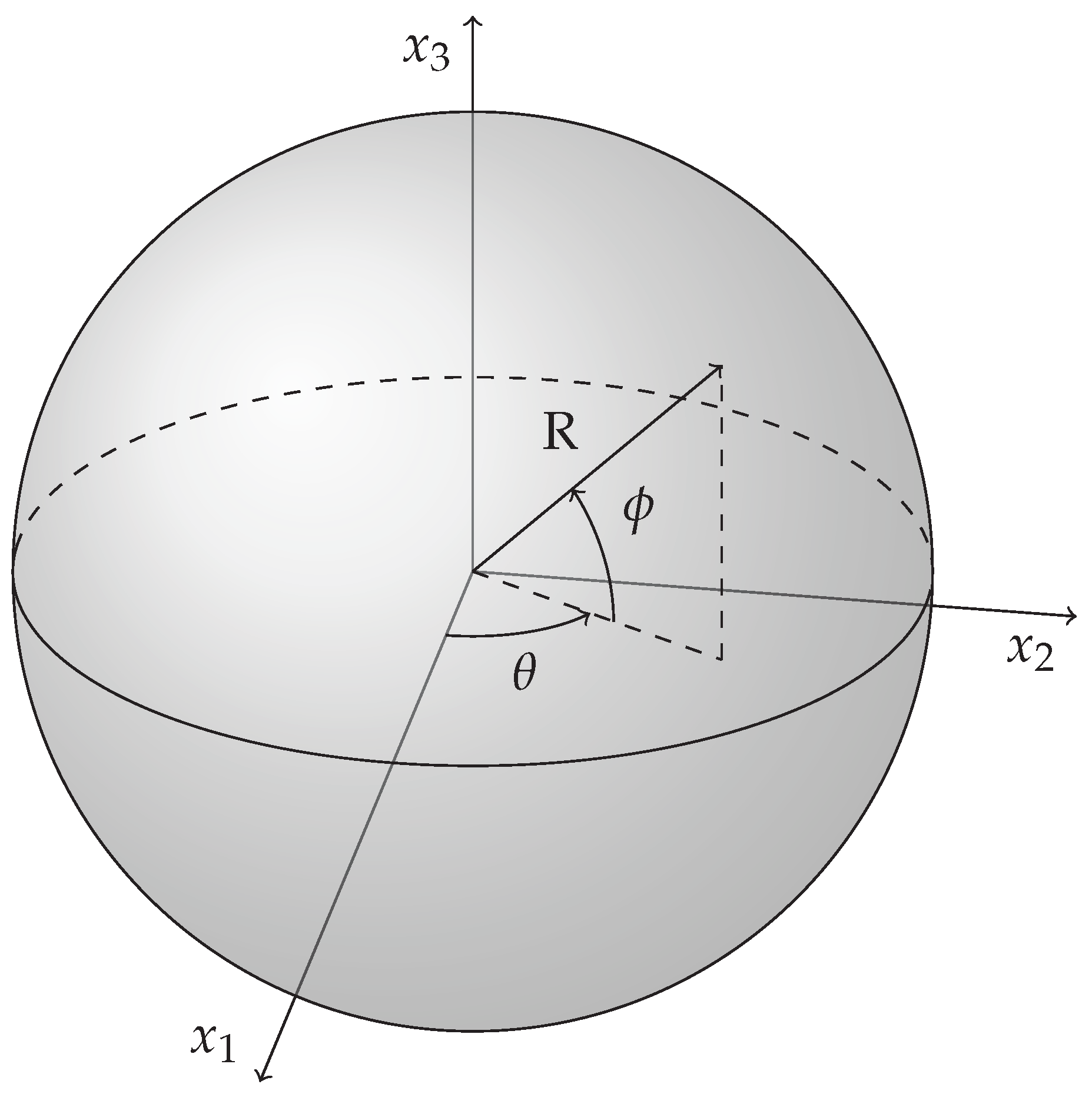
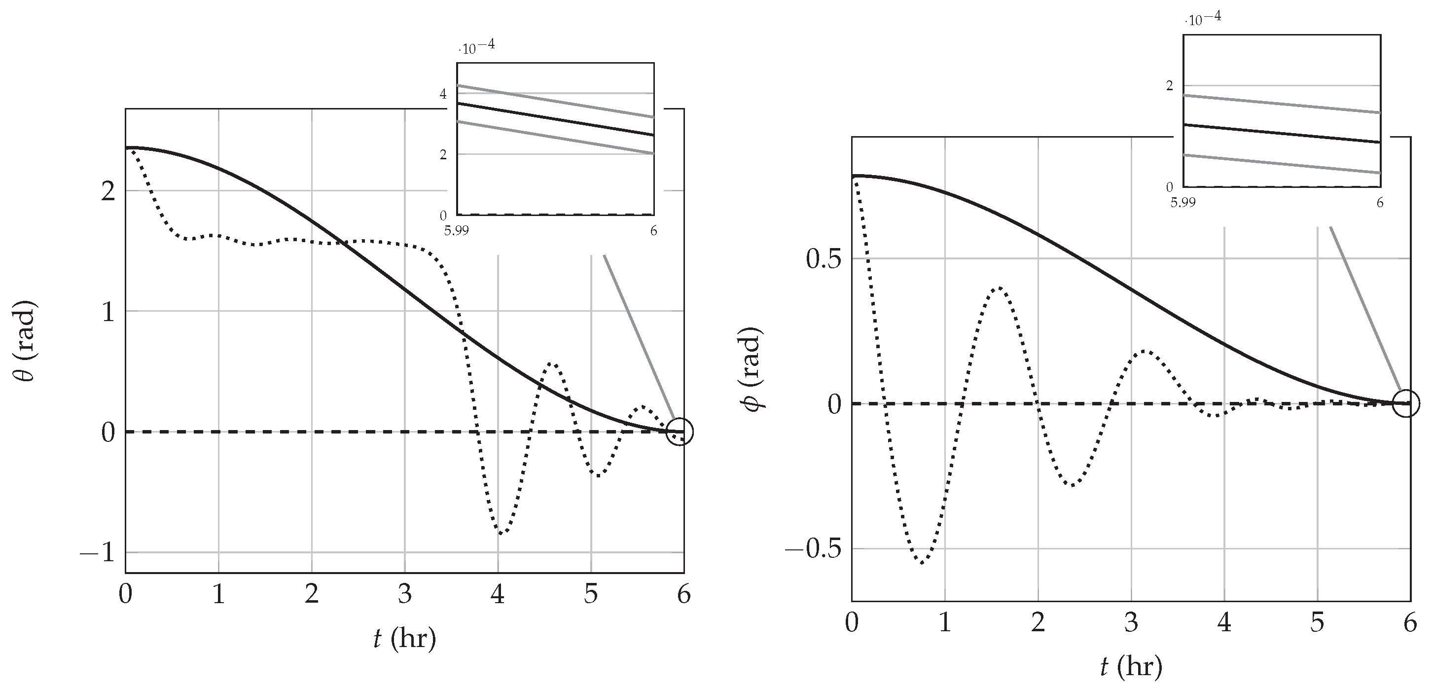
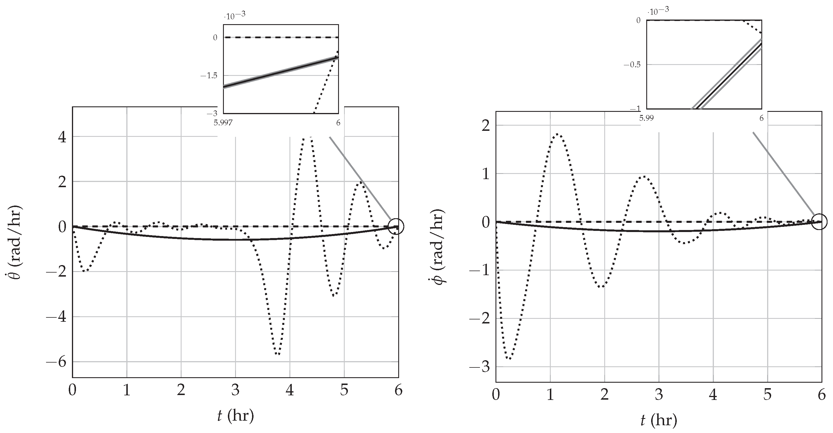
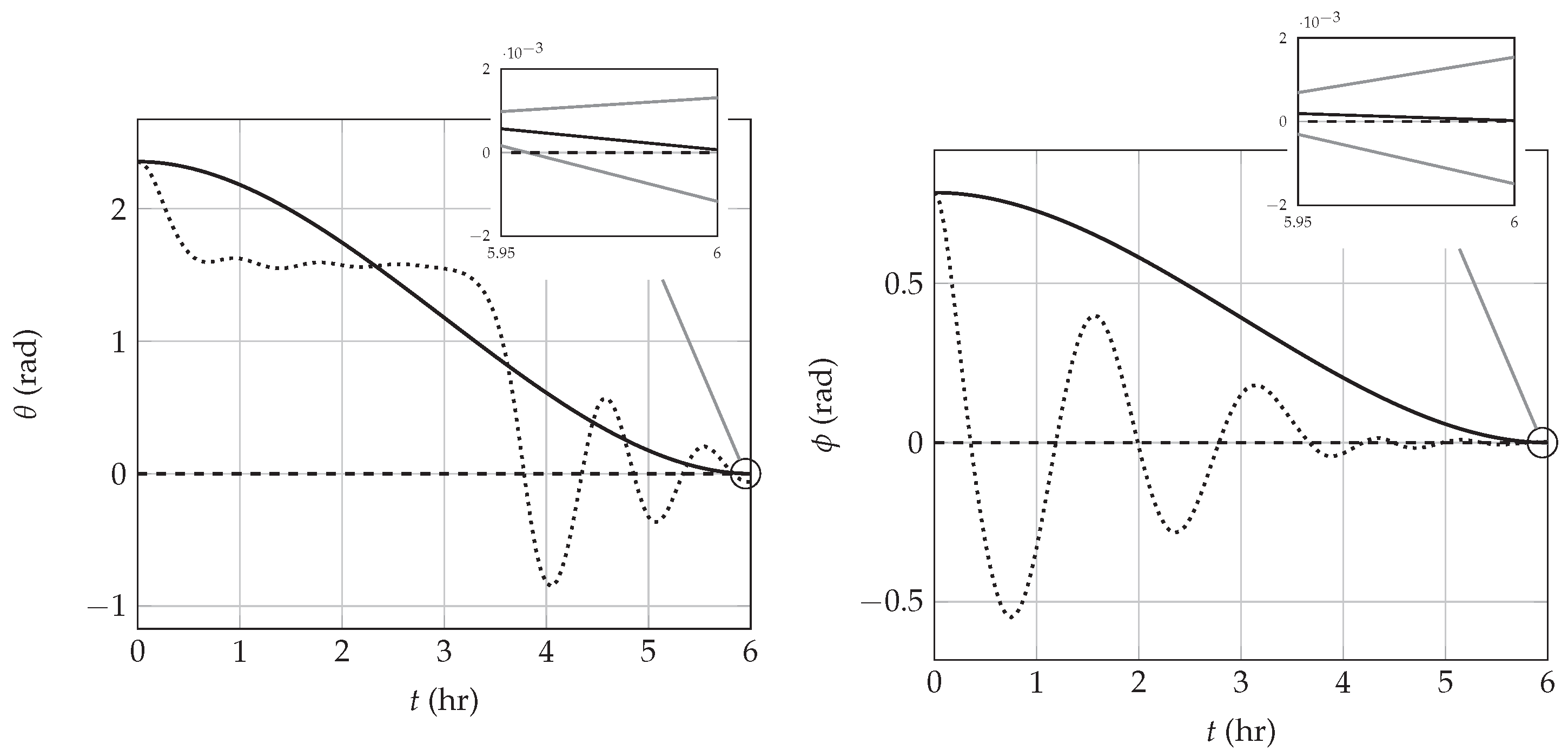
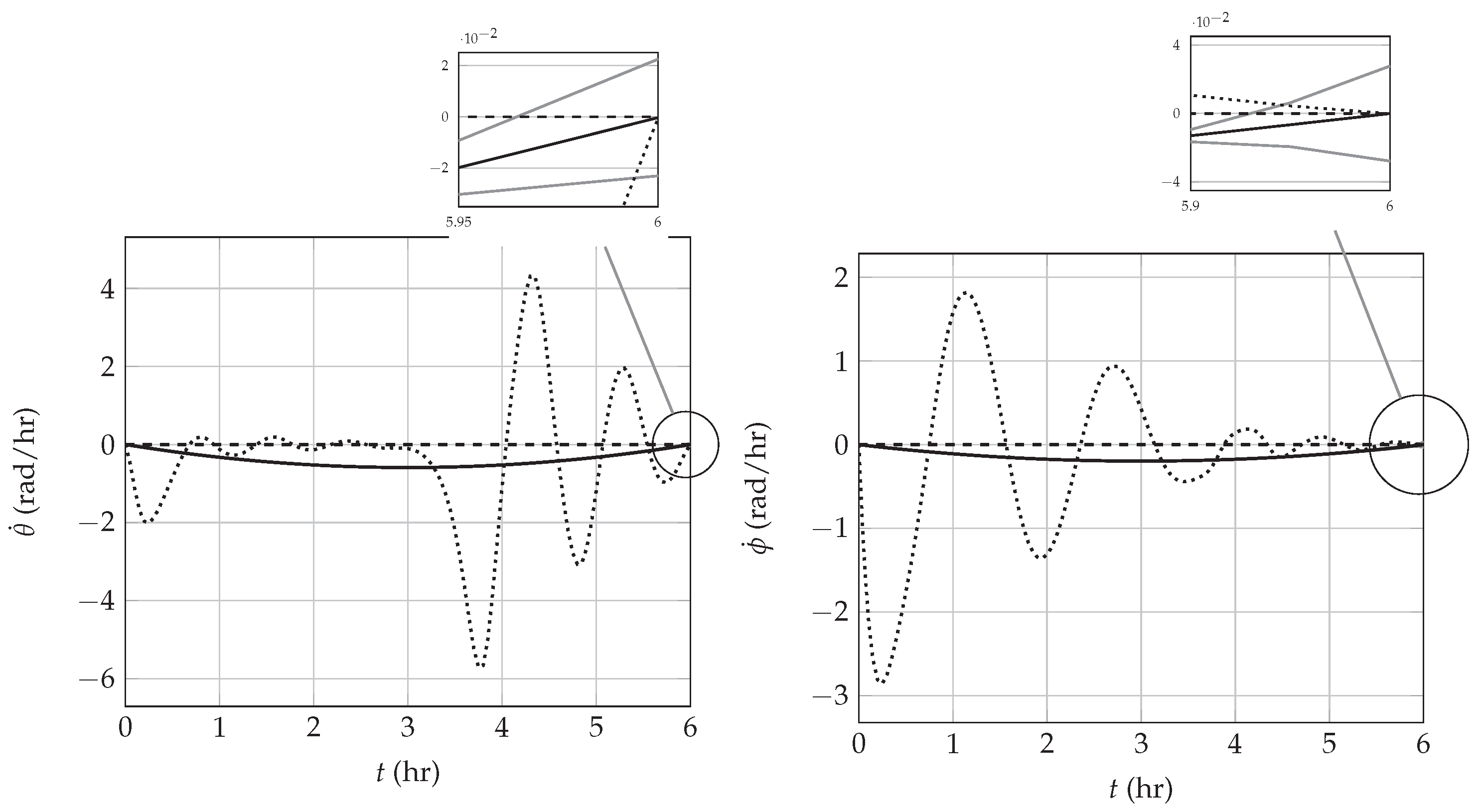
3. Spherically Constrained Relative Motion Trajectory Design

The approaches developed in Section 2 are now applied to a spherically constrained relative orbital motion problem. Variations of the problem have motivated a recent lossless convexification [28] and nonlinear dynamical analysis [36], which identified periodic and chaotic motion.

The relative motion of two spacecraft in proximity to each other in low earth orbit is described by the Clohessy–Wiltshire (CW) equations [37] as

$$\begin{array}{cc}\hfill \dot{y}& =v\hfill \\ \hfill \dot{v}& =M_{1}y+M_{2}v+\tau \hfill \end{array}$$

(17)

where $y\in {\mathbb{R}}^3$ is the relative position of the spacecraft in the local vertical local horizontal (LVLH) frame, $v\in {\mathbb{R}}^3$ is the relative velocity of the spacecraft in the LVLH frame, and $\tau \in {\mathbb{R}}^3$ is the thrust-to-mass ratio. The matrices $M_1$ and $M_2$ are

$$M_1=\left[\begin{array}{ccc}3{\omega }^2& 0& 0\\ 0& 0& 0\\ 0& 0& -{\omega }^2\end{array}\right],M_2=\left[\begin{array}{ccc}0& 2\omega & 0\\ -2\omega & 0& 0\\ 0& 0& 0\end{array}\right]$$

(18)

where the constant $\omega \in \mathbb{R}$ is the mean motion of the reference orbit. To prevent the vehicles from colliding while keeping them close together, the relative position is constrained to a sphere of radius R, i.e., $\left|\right|y\left|\right|=R$. Because of this constraint, use of a spherical coordinate system is convenient. The transformation from Cartesian to spherical coordinates is given as

$$\left[\begin{array}{c}{y}_1\\ y_2\\ y_3\end{array}\right]=r\left[\begin{array}{c}cos\left(\varphi \right)cos\left(\theta \right)\\ cos\left(\varphi \right)sin\left(\theta \right)\\ sin\left(\varphi \right)\end{array}\right]$$

(19)

where $r\in \mathbb{R}$ is the radial distance of the spacecraft from the target space object, which in the case of a spherical constraint is constant and equal to R. The spherical angles are $\varphi \in (-\pi /2,\pi /2)$ and $\theta \in [0,2\pi ]$. An illustration of the coordinate transformation is shown in Figure 1.

The thrust-to-mass ratio may be transformed from Cartesian to spherical coordinates as

$$\left[\begin{array}{c}{u}_r\\ u_{\theta }\\ u_{\varphi }\end{array}\right]=\left[\begin{array}{ccc}cos\left(\varphi \right)cos\left(\theta \right)& cos\left(\varphi \right)sin\left(\theta \right)& sin\left(\varphi \right)\\ -sin\left(\theta \right)& cos\left(\theta \right)& 0\\ -sin\left(\varphi \right)cos\left(\theta \right)& -sin\left(\varphi \right)sin\left(\theta \right)& cos\left(\varphi \right)\end{array}\right]\left[\begin{array}{c}{\tau }_1\\ {\tau }_2\\ {\tau }_3\end{array}\right].$$

(20)

Using the the defined transformations, the CW dynamics in the spherical coordinate system are

$$\begin{array}{cc}\hfill \ddot{r}& =r{\dot{\varphi }}^2+r{\omega }^2\left(3cos{\left(\varphi \right)}^{2}cos{\left(\theta \right)}^2-sin{\left(\theta \right)}^2\right)+r{\dot{\theta }}^{2}cos{\left(\varphi \right)}^2+2\omega r\dot{\theta }cos{\left(\varphi \right)}^2+u_r\hfill \end{array}$$

(21a)

$$\begin{array}{cc}\hfill \ddot{\theta }& =2(\dot{\theta }+\omega )(\dot{\varphi }tan\left(\varphi \right)-\dot{r}/r)-3{\omega }^{2}sin\left(\theta \right)cos\left(\theta \right)+u_{\theta }/\left(rcos\left(\varphi \right)\right)\hfill \end{array}$$

(21b)

$$\begin{array}{cc}\hfill \ddot{\varphi }& =-2\dot{\varphi }\dot{r}/r-sin\left(2\varphi \right){(\dot{\theta }+\omega )}^2/2-3{\omega }^{2}sin\left(\varphi \right)cos\left(\varphi \right){cos}^2\left(\theta \right)+u_{\varphi }/r.\hfill \end{array}$$

(21c)

Keeping in mind that the constraint is to stay on a spherical surface centered at the target space object, we know that $r=R$, $\dot{r}=0$ and $\ddot{r}=0$. Using this information, (21a) can be solved for the radial control $u_r$ to obtain

$$u_r=-R\left({\dot{\varphi }}^2+{\omega }^2(3cos{\left(\varphi \right)}^{2}cos{\left(\theta \right)}^2-sin{\left(\theta \right)}^2)+{\dot{\theta }}^{2}cos{\left(\varphi \right)}^2+2\omega \dot{\theta }cos{\left(\varphi \right)}^2\right).$$

(22)

The spherical controls $u_{\theta }$ and $u_{\varphi }$ may then take any values, and the relative distance between the spacecraft will remain R. Furthermore, since the $\ddot{r}$ equation is constant, it does not need to be considered for the dynamics, and the simplified equations for $\ddot{\theta }$ and $\ddot{\varphi }$ with $r=R$ and $\dot{r}=0$ are

$$\begin{array}{cc}\hfill \ddot{\theta }& =2(\dot{\theta }+\omega )\dot{\varphi }tan\left(\varphi \right)-3{\omega }^{2}sin\left(\theta \right)cos\left(\theta \right)+u_{\theta }/\left(Rcos\left(\varphi \right)\right)\hfill \\ \hfill \ddot{\varphi }& =-sin\left(2\varphi \right){(\dot{\theta }+\omega )}^2/2-3{\omega }^{2}sin\left(\varphi \right)cos\left(\varphi \right){cos}^2\left(\theta \right)+u_{\varphi }/R.\hfill \end{array}$$

(23)

Now, if a new control vector is defined as $u={[u_{\theta }/cos\left(\varphi \right),u_{\varphi }]}^{\top }$, and a state vector is defined as $x={[\theta ,\varphi ,\dot{\theta },\dot{\varphi }]}^{\top }$, the above equations can be written in the following form

$$\begin{array}{cc}\hfill \dot{x}=& \left[\begin{array}{cc}{0}_{2\times 2}& I_{2\times 2}\\ 0_{2\times 2}& 0_{2\times 2}\end{array}\right]x+\frac{1}{R}\left[\begin{array}{c}{0}_{2\times 2}\\ I_{2\times 2}\end{array}\right]u\hfill \\ \hfill & +\left[\begin{array}{c}{0}_{2\times 2}\\ 2(\dot{\theta }+\omega )\dot{\varphi }tan\left(\varphi \right)-3{\omega }^{2}sin\left(\theta \right)cos\left(\theta \right)\\ -sin\left(2\varphi \right){(\dot{\theta }+\omega )}^2/2-3{\omega }^{2}sin\left(\varphi \right)cos\left(\varphi \right){cos}^2\left(\theta \right)\end{array}\right].\hfill \end{array}$$

(24)

This nonlinear system is in the form of (1) with the system matrices being

$$A=\left[\begin{array}{cc}{0}_{2\times 2}& I_{2\times 2}\\ 0_{2\times 2}& 0_{2\times 2}\end{array}\right],B=\frac{1}{R}\left[\begin{array}{c}{0}_{2\times 2}\\ I_{2\times 2}\end{array}\right],E=\left[\begin{array}{c}{0}_{2\times 2}\\ I_{2\times 2}\end{array}\right]$$

(25)

and the nonlinear function $\eta$ given by

$$\eta (\theta ,\varphi ,\dot{\theta },\dot{\varphi })=\left[\begin{array}{c}2(\dot{\theta }+\omega )\dot{\varphi }tan\left(\varphi \right)-3{\omega }^{2}sin\left(\theta \right)cos\left(\theta \right)\\ -sin\left(2\varphi \right){(\dot{\theta }+\omega )}^2/2-3{\omega }^{2}sin\left(\varphi \right)cos\left(\varphi \right){cos}^2\left(\theta \right)\end{array}\right].$$

(26)

For numerical purposes, the radius R of the sphere is 100 m and the mean motion $\omega$ is 4 rad/h, which corresponds to a low earth orbit with a period of $\pi /2$ h. The dynamics in (24) are discretized according to the procedure in Appendix A with $\Delta t=0.05$ h to obtain

$$A_d=\left[\begin{array}{cccc}1& 0& 0.05& 0\\ 0& 1& 0& 0.05\\ 0& 0& 1& 0\\ 0& 0& 0& 1\end{array}\right],B_d=\left[\begin{array}{cc}0.0125& 0\\ 0& 0.0125\\ 0.5& 0\\ 0& 0.5\end{array}\right]\times {10}^{-3},E_d=\left[\begin{array}{cc}0.00125& 0\\ 0& 0.00125\\ 0.05& 0\\ 0& 0.05\end{array}\right].$$

(27)

The initial relative position of the spacecraft is defined as ${\theta }_0=3\pi /4$ rad and ${\varphi }_0=\pi /4$ rad with initial relative velocity of zero. The desired final relative position of the spacecraft is ${\theta }_f={\varphi }_f=0$ rad and the desired final relative velocity is zero. This maneuver is to be completed in 6 h. With the chosen time step as $0.05$ h, N becomes 120. The vertices for the bounding polytope of the nonlinearity are chosen as (all in rad/h²)

$${\delta }_1=\left[\begin{array}{c}-35\\ -42\end{array}\right],{\delta }_2=\left[\begin{array}{c}-35\\ +42\end{array}\right],{\delta }_3=\left[\begin{array}{c}+35\\ -42\end{array}\right],{\delta }_4=\left[\begin{array}{c}+35\\ +42\end{array}\right].$$

(28)

With this in place, Theorem 1 may be applied to generate feasible solutions to the nonlinear trajectory design and control problem. First, the ‘constrained approach’ is used, which is followed by the ‘resetting approach’. Both of the solutions are compared against a solution that was achieved by solving a non-convex optimization problem using MATLAB’s [38] fmincon solver. The ‘constrained’ and ‘resetting’ solutions are used as initial guesses for the non-convex solver.

3.1. Constrained Approach

In this approach, the constraints in (7) are incorporated into an optimization problem. The second-order cone programming (SOCP) problem to be solved is

$$\begin{array}{cc}\hfill \underset{u}{min}& \sum _{i=1}^4\left(\sum _{k=0}^{N-1}{10}^{-12}{\parallel u_i\left[k\right]\parallel }^2+{\parallel x_i\left[N\right]-x_f\parallel }^2\right)\hfill \end{array}$$

(29a)

$$\begin{array}{cc}\hfill \mathrm{s}.\mathrm{t}.& x_i[k+1]=A_d{x}_i\left[k\right]+B_d{u}_i\left[k\right]+E_d{\delta }_i,i=1,\dots ,4,k=0,\dots ,N-1\hfill \end{array}$$

(29b)

$$\begin{array}{cc}\hfill & x_i\left[0\right]=x_0,i=1,\dots ,4\hfill \end{array}$$

(29c)

$$\begin{array}{cc}\hfill & \mathrm{Equation}\left(7\right)\mathrm{with}⋎={[4,4,4,4]}^{\top }\mathrm{and}⋏={[2,3,2,3]}^{\top },k=1,\dots ,N\hfill \end{array}$$

(29d)

The cost function in (29a) has two quadratic terms. The first term penalizes the control inputs of the auxiliary LTI systems. This term is not needed; it serves to regularize or smooth the resulting solutions. The second term penalizes errors in the final state. Weights multiplying the terms have been chosen based on their magnitudes. The control inputs for the auxiliary LTI systems are on the order of ${10}^4$, whereas the final state error gets very close to zero; therefore, the multiplier for the final state error is chosen to be significantly larger than that for the control inputs. The dynamics of the auxiliary LTI systems are enforced in (29b) with initial conditions in (29c). The ordering constraint (7) of Theorem 1 is enforced in (29d). Note that other orderings can be used, and it is not required for one ordering to be enforced at all k. The user is free to choose the ordering.

Solving the optimization problem (29) took 1.14 s on a laptop with a 2.30 GHz Intel i7 processor using Gurobi [39] in MATLAB [38] through YALMIP [40]. The same setup was used for all the computations in the following sections as well.

Figure 2 shows the relative angular displacement trajectories of the spacecraft and Figure 3 shows the relative angular velocity trajectories of the spacecraft. In the figures, the linear system trajectories are covered by the actual nonlinear system trajectories; however, the nonlinear system trajectory is between the upper and lower bounds of the linear system trajectories. From inspection of the magnified inset, it is evident that the final angular displacements are on the order of ${10}^{-4}$ rad corresponding to a final position error on the centimeter level.

3.2. Resetting Approach

In this section, the constrained relative motion problem is solved using the ’resetting approach’ described in Algorithm 1. The SOCP problem used to find control solutions in Line 3 of Algorithm 1 is the same as (29) but with (29d) removed. The resets are performed as described in Algorithm 1.

The results are shown in Figure 4 and Figure 5. The results are similar to those shown in Figure 2 and Figure 3, except that towards the end of the time horizon, the angular velocity trajectories of the linear systems diverge from the desired final velocity. The noticeable difference is that designing this controller requires a solution to 11 SOCP problems as there were 10 resets due to violations of the ordering constraint in 7. On average, solving each problem required 0.17 s for a total solve time of 1.87 s. The number of variables in each optimization problem also reduces on each reset as the time horizon gets shorter.

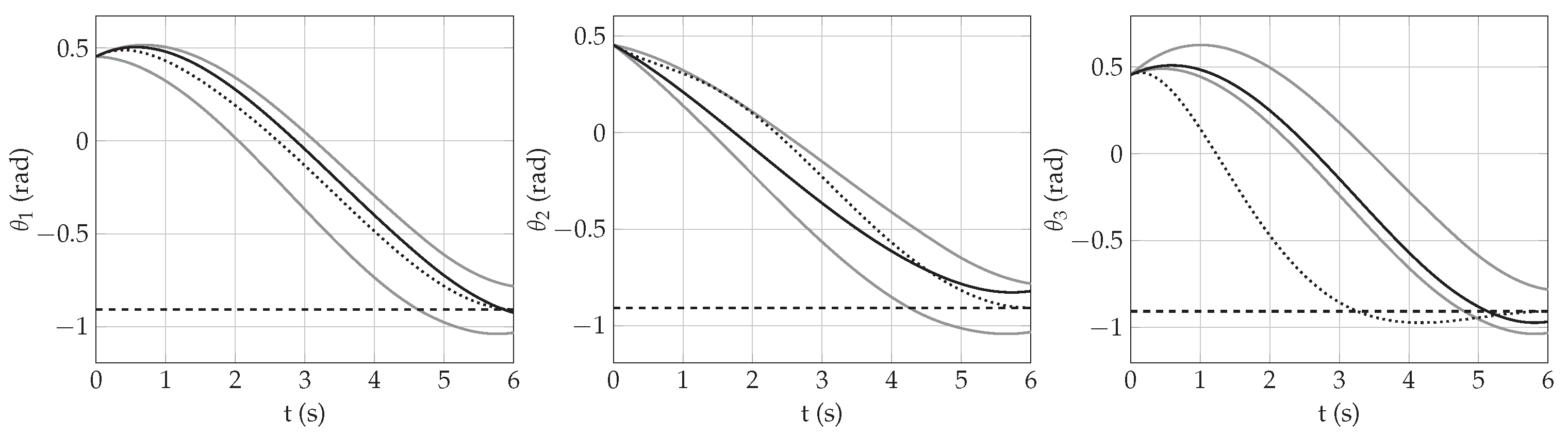
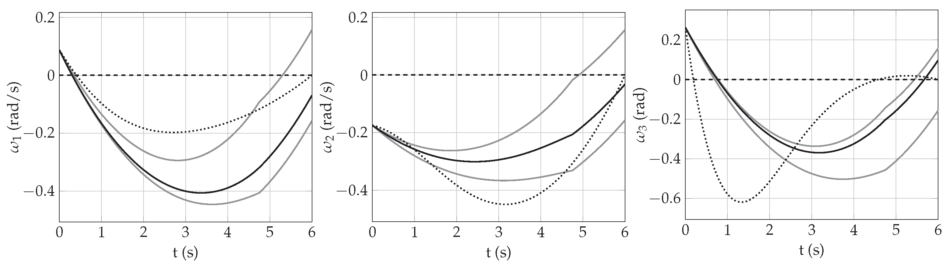
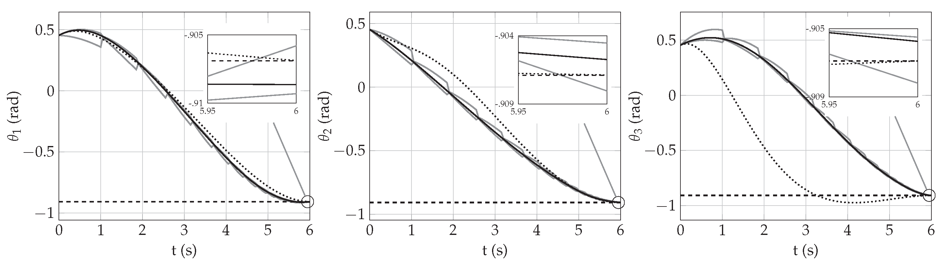
4. Spacecraft Attitude Control

The approaches developed in Section 2 are now applied to a spacecraft attitude control problem. To represent the attitude of a spacecraft, a rotation vector $\theta =\alpha e\in {\mathbb{R}}^3$ is used. The unit vector $e\in {\mathbb{R}}^3$ is the Euler rotation axis and $\alpha \in \mathbb{R}$ is the angular displacement. To derive the kinematics of the spacecraft attitude, a quaternion $q\in {\mathbb{R}}^4$ is defined representing the spacecraft attitude as [41]

$$q=\left[\begin{array}{c}\frac{1}{\alpha }sin(\alpha /2)\theta \\ cos(\alpha /2)\end{array}\right].$$

(30)

Taking the time derivative leads to

$$\dot{q}=\left[\begin{array}{c}\frac{1}{\alpha }sin(\alpha /2)\dot{\theta }\\ 0\end{array}\right]+\left[\begin{array}{c}\left(-\frac{1}{{\alpha }^2}sin(\alpha /2)+\frac{1}{2\alpha }cos(\alpha /2)\right)\dot{\alpha }\theta \\ -\frac{1}{2}sin(\alpha /2)\dot{\alpha }\end{array}\right].$$

(31)

It is also well-known that the quaternion kinematics can be written as [42]

$$\begin{array}{cc}\hfill \dot{q}& =\frac{1}{2}\left[\begin{array}{c}{q}_4\omega +q_{1:3}\times \omega \\ -q_{1:3}^{\top }\omega \end{array}\right]\hfill \end{array}$$

(32)

$$\begin{array}{cc}\hfill & \hspace{1em}\hspace{1em}\hspace{1em}\hspace{1em}\hspace{1em}\hspace{1em}\hspace{1em}\hspace{1em}=\frac{1}{2}\left[\begin{array}{c}cos(\alpha /2)\omega -\frac{1}{\alpha }sin(\alpha /2)\theta \times \omega \\ -\frac{1}{\alpha }sin(\alpha /2){\theta }^{\top }\omega \end{array}\right]\hfill \end{array}$$

(33)

where $\omega \in {\mathbb{R}\mathbb{R}}^3$ is the attitude rate of the spacecraft expressed in its body frame. Comparing the last element of (31) and (33) gives an expression for $\dot{\alpha }$ as $\dot{\alpha }={\alpha }^{-1}{\theta }^{\top }\omega$. Comparing the first three elements of (31) and (33), substituting the expression of $\dot{\alpha }$, and solving for $\dot{\theta }$, gives

$$\dot{\theta }=\left(\frac{1}{\alpha }-\frac{1}{2}cot(\alpha /2)\right)\frac{1}{\alpha }{\theta }^{\top }\omega \theta +\frac{1}{2}\left(\alpha cot(\alpha /2)\omega +\theta \times \omega \right).$$

(34)

Subtracting and adding ${\alpha }^{-2}{\theta }^{\top }\theta \omega$ on the right-hand side, using the vector triple product, and noting that $\alpha =\parallel \theta \parallel$ (provided $0<\alpha <2\pi$), simplifies the above to

$$\dot{\theta }=\omega +\frac{1}{2}\theta \times \omega +\frac{1}{{\parallel \theta \parallel }^2}\left(1-\frac{\parallel \theta \parallel }{2}cot\left(\right|\left|\theta \right||/2)\right)\theta \times (\theta \times \omega ).$$

(35)

The attitude dynamics of the spacecraft can be derived from Euler’s equations [42]. Assuming that the only external torque affecting the system is a control torque $\tau \in {\mathbb{R}}^3$, the dynamics are

$$\dot{\omega }=J^{-1}\left(\omega \times \left(J\omega \right)+\tau \right)$$

(36)

where J is a moment of inertia of the spacecraft about its center of mass represented in the body frame. Defining the state vector as $x={[{\theta }^{\top },{\omega }^{\top }]}^{\top }\in {\mathbb{R}}^6$, Equations (35) and (36) can be written as

$$\begin{array}{cc}\hfill \dot{x}=& \left[\begin{array}{cc}{0}_{3\times 3}& I_{3\times 2}\\ 0_{3\times 3}& 0_{3\times 3}\end{array}\right]x+\left[\begin{array}{c}{0}_{3\times 3}\\ J^{-1}\end{array}\right]\tau \hfill \\ \hfill & +\left[\begin{array}{cc}{I}_{3\times 3}& 0_{3\times 3}\\ 0_{3\times 3}& J^{-1}\end{array}\right]\left[\begin{array}{c}\frac{1}{2}\theta \times \omega +\frac{1}{{\parallel \theta \parallel }^2}\left(1-\frac{\parallel \theta \parallel }{2}cot\left(\right|\left|\theta \right||/2)\right)\theta \times (\theta \times \omega )\\ \omega \times \left(J\omega \right)\end{array}\right].\hfill \end{array}$$

(37)

To simplify the nonlinear effects, it is assumed that the rate vector $\omega$ is known from navigation and available for feedback linearization. Upon defining the control $\tau =u-\omega \times \left(J\omega \right)$, the nonlinear system is

$$\begin{array}{cc}\hfill \dot{x}=& \left[\begin{array}{cc}{0}_{3\times 3}& I_{3\times 2}\\ 0_{3\times 3}& 0_{3\times 3}\end{array}\right]x+\left[\begin{array}{c}{0}_{3\times 3}\\ J^{-1}\end{array}\right]u\hfill \\ \hfill & +\left[\begin{array}{c}{I}_{3\times 3}\\ 0_{3\times 3}\end{array}\right]\left[\begin{array}{c}\frac{1}{2}\theta \times \omega +\frac{1}{{\parallel \theta \parallel }^2}\left(1-\frac{\parallel \theta \parallel }{2}cot\left(\right|\left|\theta \right||/2)\right)\theta \times (\theta \times \omega )\end{array}\right].\hfill \end{array}$$

(38)

Feedback linearization has the effect of reducing the dimension of the nonlinearity from six to three, which in turn reduces the dimension of the bounding convex polytope.

This nonlinear system is in the form of (1), with the system matrices being

$$A=\left[\begin{array}{cc}{0}_{3\times 3}& I_{3\times 2}\\ 0_{3\times 3}& 0_{3\times 3}\end{array}\right],B=\left[\begin{array}{c}{0}_{3\times 3}\\ J^{-1}\end{array}\right],E=\left[\begin{array}{c}{I}_{3\times 3}\\ 0_{3\times 3}\end{array}\right]$$

(39)

and the nonlinear function $\eta$ given by

$$\eta (\theta ,\omega )=\frac{1}{2}\theta \times \omega +\frac{1}{{\parallel \theta \parallel }^2}\left(1-\frac{\parallel \theta \parallel }{2}cot\left(\right|\left|\theta \right||/2)\right)\theta \times (\theta \times \omega ).$$

(40)

For numerical purposes, the spacecraft is assumed to have a cylindrical shape with constant density. The radius of the spacecraft is $r=0.25$ m, height $h=0.5$ m, and mass $m=100$ kg. The body z-axis is defined to be aligned with the axis of the cylinder. The moment of inertia matrix is then given as $J=\mathrm{diag}\{J_{xx},J_{yy},J_{zz}\}$, where $J_{xx}=J_{yy}=\frac{1}{4}m{r}^2+\frac{1}{12}m{h}^2$ and $J_{zz}=\frac{1}{2}m{r}^2$. The dynamics in (37) are discretized according to the procedure in Appendix A with $\Delta t=0.05$ sec to obtain

$$\begin{array}{cc}\hfill & A_d=\left[\begin{array}{cccccc}1& 0& 0& 0.05& 0& 0\\ 0& 1& 0& 0& 0.05& 0\\ 0& 0& 1& 0& 0& 0.05\\ 0& 0& 0& 1& 0& 0\\ 0& 0& 0& 0& 1& 0\\ 0& 0& 0& 0& 0& 1\end{array}\right],B_d=\left[\begin{array}{ccc}0.343& 0& 0\\ 0& 0.343& 0\\ 0& 0& 0.4\\ 13.7& 0& 0\\ 0& 13.7& 0\\ 0& 0& 16\end{array}\right]\times {10}^{-3},\hfill \\ \hfill & E_d=\left[\begin{array}{ccc}0.05& 0& 0\\ 0& 0.05& 0\\ 0& 0& 0.05\\ 0& 0& 0\\ 0& 0& 0\\ 0& 0& 0\end{array}\right].\hfill \end{array}$$

(41)

The initial attitude of the spacecraft is given with an axis of rotation of $\frac{1}{\sqrt{3}}{[1,1,1]}^{\top }$ and angle ${45}^{\circ }$. The desired final attitude is given by an axis of rotation of $-\frac{1}{\sqrt{3}}{[1,1,1]}^{\top }$ and angle ${90}^{\circ }$. The initial angular velocity of the spacecraft is $[5,-10,15]{}^{\circ }/\mathrm{s}$ and the desired final angular velocity is zero. The maneuver is to be performed in 6 s. With the chosen time step of 0.05 s, N becomes 120. The vertices for the bounding polytope of the nonlinearity are chosen as (all in rad/s)

$$\begin{array}{c}\hfill {\delta }_1=\left[\begin{array}{c}-0.1\\ -0.1\\ -0.1\end{array}\right],{\delta }_2=\left[\begin{array}{c}-0.1\\ -0.1\\ +0.1\end{array}\right],{\delta }_3=\left[\begin{array}{c}-0.1\\ +0.1\\ -0.1\end{array}\right],{\delta }_4=\left[\begin{array}{c}-0.1\\ +0.1\\ +0.1\end{array}\right],\\ \hfill {\delta }_5=\left[\begin{array}{c}+0.1\\ -0.1\\ -0.1\end{array}\right],{\delta }_6=\left[\begin{array}{c}+0.1\\ -0.1\\ +0.1\end{array}\right],{\delta }_7=\left[\begin{array}{c}+0.1\\ +0.1\\ -0.1\end{array}\right],{\delta }_8=\left[\begin{array}{c}+0.1\\ +0.1\\ +0.1\end{array}\right].\end{array}$$

(42)

Again, Theorem 1 may be applied to generate feasible solutions to the nonlinear trajectory design and control problem. The ‘constrained’ and ‘resetting’ approaches are compared against a solution that was achieved by solving a non-convex optimization problem using MATLAB’s [38] fmincon solver with the initial guesses obtained from the ‘constrained’ and ‘resetting solutions’.

4.1. Constrained Approach

In this approach, the constraints in (7) are incorporated into an optimization problem. The second-order cone programming (SOCP) problem to be solved is

$$\begin{array}{cc}\hfill \underset{u}{min}& \sum _{i=1}^8\left(\sum _{k=0}^{N-1}{10}^{-8}{\parallel u_i\left[k\right]\parallel }^2+{\parallel x_i\left[N\right]-x_f\parallel }^2\right)\hfill \end{array}$$

(43a)

$$\begin{array}{cc}\hfill \mathrm{s}.\mathrm{t}.& x_i[k+1]=A_d{x}_i\left[k\right]+B_d{u}_i\left[k\right]+E_d{\delta }_i,i=1,\dots ,8,k=0,\dots ,N-1\hfill \end{array}$$

(43b)

$$\begin{array}{cc}\hfill & x_i\left[0\right]=x_0,i=1,\dots ,8\hfill \end{array}$$

(43c)

$$\begin{array}{cc}\hfill & \mathrm{Equation}\left(7\right)\mathrm{with}⋎={[4,6,7,8,8,8]}^{\top },k=1,\dots ,N\hfill \\ \hfill & ⋏={[8,8,8,4,6,7]}^{\top },k=1,\dots ,N\hfill \end{array}$$

(43d)

Due to different scaling between the auxiliary system control magnitudes and errors between actual and desired final states compared with the relative motion problem of the previous section, the weight on the control term was set to 10${}^{-8}$. As before, the control penalty is not needed but has a regularizing effect. The dynamics of the auxiliary LTI systems are enforced in (43b) with initial conditions in (43c). The ordering constraint (7) of Theorem 1 is enforced in (43d).

Solving the SOCP problem took $1.09$ s. Figure 6 shows the attitude of the spapecraft with the dashed line as the desired final attitude. Figure 7 shows the angular velocity of the spacecraft. It can be seen in these figures that the nonlinear system does not arrive exactly to the desired final state but stays between the upper and lower bounding linear systems. The magnitude of error between the desired final rotation vector and the final rotation vector of the nonlinear system is $0.107$ rad. However, the average magnitude of error between the desired final rotation vector and the final rotation vectors of the linear auxiliary systems is $0.217$ rad. Since the linear auxiliary systems provide the limits for the nonlinear system trajectories, better performance is desired and is investigated as part of the ‘resetting approach’.

4.2. Resetting Approach

In this section, the attitude control problem is solved using the ’resetting approach’ described in Algorithm 1. The SOCP problem used to find control solutions in Line 3 of Algorithm 1 is the same as (43) but with (43d) removed. The resets are performed as described in Algorithm 1.

Figure 8 shows the attitude of the spacecraft with the dashed line as the desired final attitude. Figure 9 shows the angular velocity of the spacecraft. It can be seen on these figures that the resetting controller seems to perform significantly better than the constrained controller in the previous section especially when comparing the errors between the desired final attitude and the actual final attitude. The magnitude of the error between the desired final rotation vector and the final rotation vector of the nonlinear system is $2.17\times {10}^{-3}$ rad. Even the average magnitude of the error between the desired final rotation vector and the final rotation vectors of the auxiliary systems is only $2.9\times {10}^{-3}$ rad. These are significantly lower compared with the final attitude errors reached with the constrained controller. The design of this controller required solving 20 SOCP problems with an average solution time of $0.233$ s for a total solver time of $4.67$ s. The resets are also easily noticeable because of the saw-blade-like linear system trajectories.

5. Summary and Conclusions

Convex optimization-based techniques for trajectory design and control of nonlinear systems with convex state and control constraints were presented. The techniques apply to systems for which the range of the nonlinear dynamics function is contained in a convex polytope. Sufficient conditions for the problem to be solvable by a single convex program were given. The theoretical results were applied to two practical problems in aerospace engineering: a constrained relative orbital motion problem and an attitude control problem. Solution times were on the order of seconds. An alternative ‘resetting approach’ was also introduced that applies to problems not satisfying the sufficient conditions or when the so-called ordering constraint is difficult to implement. This resetting approach requires the solution of multiple convex programs; however, solve times remained on the order of seconds. Both methods were compared against a non-convex optimization solution as well. It is concluded that this technique is rigorous and is a practical means of solving nonlinear trajectory design and control problems efficiently.

References

1. Flores-Abad, A.; Ma, O.; Pham, K.; Ulrich, S. A review of space robotics technologies for on-orbit servicing. Prog. Aerosp. Sci. 2014, 68, 1–26. [Google Scholar] [CrossRef] [Green Version]
2. Li, W.J.; Cheng, D.Y.; Liu, X.G.; Wang, Y.B.; Shi, W.H.; Tang, Z.X.; Gao, F.; Zeng, F.M.; Chai, H.Y.; Luo, W.B.; et al. On-orbit service (OOS) of spacecraft: A review of engineering developments. Prog. Aerosp. Sci. 2019, 108, 32–120. [Google Scholar] [CrossRef]
3. Tsuda, Y.; Yoshikawa, M.; Abe, M.; Minamino, H.; Nakazawa, S. System design of the Hayabusa 2—Asteroid sample return mission to 1999 JU3. Acta Astronaut. 2013, 91, 356–362. [Google Scholar] [CrossRef]
4. Gaudet, B.; Linares, R.; Furfaro, R. Terminal adaptive guidance via reinforcement meta-learning: Applications to autonomous asteroid close-proximity operations. Acta Astronaut. 2020, 171, 1–13. [Google Scholar] [CrossRef] [Green Version]
5. D’Amico, S.; Benn, M.; Jørgensen, J.L. Pose estimation of an uncooperative spacecraft from actual space imagery. Int. J. Space Sci. Eng. 2014, 2, 171–189. [Google Scholar]
6. Stastny, N.B.; Geller, D.K. Autonomous optical navigation at Jupiter: A linear covariance analysis. J. Spacecr. Rocket. 2008, 45, 290–298. [Google Scholar] [CrossRef] [Green Version]
7. Bradley, N.; Olikara, Z.; Bhaskaran, S.; Young, B. Cislunar navigation accuracy using optical observations of natural and artificial targets. J. Spacecr. Rocket. 2020, 57, 777–792. [Google Scholar] [CrossRef]
8. Curtis, H. Orbital Mechanics for Engineering Students, 2nd ed.; Butterworth-Heinemann: Oxford, UK, 2009. [Google Scholar]
9. Khalil, H.K. Nonlinear Systems; Pearson: New York, NY, USA, 2001. [Google Scholar]
10. Harris, M.W.; Açıkmeşe, B. Maximum divert for planetary landing using convex optimization. J. Optim. Theory Appl. 2014, 162, 975–995. [Google Scholar] [CrossRef]
11. Brunton, S.L.; Brunton, B.W.; Proctor, J.L.; Kutz, J.N. Koopman Invariant Subspaces and Finite Linear Representations of Nonlinear Dynamical Systems for Control. PLoS ONE 2016, 11, e0150171. [Google Scholar] [CrossRef] [Green Version]
12. Yeung, E.; Kundu, S.; Hodas, N. Learning deep neural network representations for Koopman operators of nonlinear dynamical systems. In Proceedings of the 2019 American Control Conference (ACC), Philadelphia, PA, USA, 10–12 July 2019; pp. 4832–4839. [Google Scholar]
13. Brunton, S.L.; Kutz, J.N. Data-Driven science and Engineering: Machine Learning, Dynamical Systems, and Control; Cambridge University Press: Cambridge, UK, 2022. [Google Scholar]
14. Lusch, B.; Kutz, J.N.; Brunton, S.L. Deep learning for universal linear embeddings of nonlinear dynamics. Nat. Commun. 2018, 9, 1–10. [Google Scholar] [CrossRef] [Green Version]
15. Rugh, W.J.; Shamma, J.S. Research on gain scheduling. Automatica 2000, 36, 1401–1425. [Google Scholar] [CrossRef]
16. Sename, O.; Gaspar, P.; Bokor, J. Robust Control and Linear Parameter Varying Approaches: Application to Vehicle Dynamics; Springer: Berlin/Heidelberg, Germany, 2013; Volume 437. [Google Scholar]
17. He, T. Smooth Switching LPV Control and Its Applications; Michigan State University: East Lansing, MI, USA, 2019. [Google Scholar]
18. Jansson, O.; Harris, M.W. Nonlinear Control Algorithm for Systems with Convex Polytope Bounded Nonlinearities. In Proceedings of the 2022 Intermountain Engineering, Technology and Computing (IETC), Orem, UT, USA, 13–14 May 2022; pp. 1–6. [Google Scholar]
19. Malisoff, M.; Sontag, E.D. Universal formulas for feedback stabilization with respect to Minkowski balls. Syst. Control Lett. 2000, 40, 247–260. [Google Scholar] [CrossRef]
20. Pylorof, D.; Bakolas, E. Nonlinear control under polytopic input constraints with application to the attitude control problem. In Proceedings of the 2015 American Control Conference (ACC), Chicago, IL, USA, 1–3 July 2015; pp. 4555–4560. [Google Scholar] [CrossRef]
21. Ames, A.D.; Coogan, S.; Egerstedt, M.; Notomista, G.; Sreenath, K.; Tabuada, P. Control Barrier Functions: Theory and Applications. In Proceedings of the 2019 18th European Control Conference (ECC), Naples, Italy, 25–28 June 2019; pp. 3420–3431. [Google Scholar] [CrossRef] [Green Version]
22. Harris, M.W. Lossless Convexification of Optimal Control Problems; The University of Texas at Austin: Austin, TX, USA, 2014. [Google Scholar]
23. Açıkmeşe, B.; Blackmore, L. Lossless convexification for a class of optimal control problems with nonconvex control constraints. Automatica 2011, 47, 341–347. [Google Scholar] [CrossRef]
24. Kunhippurayil, S.; Harris, M.W.; Jansson, O. Lossless Convexification of Optimal Control Problems with Annular Control Constraints. Automatica 2021, 133, 109848. [Google Scholar] [CrossRef]
25. Harris, M.W.; Açıkmeşe, B. Lossless convexification of non-convex optimal control problems for state constrained linear systems. Automatica 2014, 50, 2304–2311. [Google Scholar] [CrossRef]
26. Harris, M.W.; Açıkmeşe, B. Lossless Convexification for a Class of Optimal Control Problems with Linear State Constraints. In Proceedings of the 52nd IEEE Conference on Decision and Control, Florence, Italy, 10–13 December 2013. [Google Scholar]
27. Harris, M.W.; Açıkmeşe, B. Lossless Convexification for a Class of Optimal Control Problems with Quadratic State Constraints. In Proceedings of the 2013 American Control Conference, Washington, DC, USA, 17–19 June 2013. [Google Scholar]
28. Woodford, N.; Harris, M.W. Geometric Properties of Time Optimal Controls with State Constraints Using Strong Observability. IEEE Trans. Autom. Control 2022, 67, 6881–6887. [Google Scholar] [CrossRef]
29. Harris, M.W. Optimal Control on Disconnected Sets using Extreme Point Relaxations and Normality Approximations. IEEE Trans. Autom. Control 2021, 66, 6063–6070. [Google Scholar] [CrossRef]
30. Kunhippurayil, S.; Harris, M.W. Strong observability as a sufficient condition for non-singularity and lossless convexification in optimal control with mixed constraints. Control Theory Technol. 2022, 20, 475–487. [Google Scholar] [CrossRef]
31. Blackmore, L.; Açıkmeşe, B.; Carson, J.M. Lossless convexification of control constraints for a class of nonlinear optimal control problems. Syst. Control Lett. 2012, 61, 863–871. [Google Scholar] [CrossRef]
32. Lu, P.; Liu, X. Autonomous trajectory planning for rendezvous and proximity aperations by conic optimization. J. Guid. Control Dyn. 2013, 36, 375–389. [Google Scholar] [CrossRef]
33. Lu, P. Introducing computational guidance and control. J. Guid. Control Dyn. 2017, 40, 193. [Google Scholar] [CrossRef]
34. Liu, X.; Lu, P.; Pan, B. Survey of convex optimization for aerospace applications. Astrodynamics 2017, 1, 23–40. [Google Scholar] [CrossRef]
35. Liu, X.; Lu, P. Solving nonconvex optimal control problems by convex optimization. J. Guid. Control Dyn. 2014, 37, 750–765. [Google Scholar] [CrossRef]
36. Harris, M.W.; Woodford, N.T. Equilibria, Periodicity, and Chaotic Behavior in Spherically Constrained Relative Orbital Motion. Nonlinear Dyn. 2023, 111, 1–17. [Google Scholar] [CrossRef]
37. Clohessy, W.; Wiltshire, R. Terminal guidance system for satellite rendezvous. J. Aerosp. Sci. 1960, 27, 653–658. [Google Scholar] [CrossRef]
38. MATLAB 2021a; The Mathworks, Inc.: Natick, MA, USA, 2021.
39. Gurobi Optimization, LLC. Gurobi Optimizer Reference Manual; Gurobi Optimization, LLC: Houston, TX, USA, 2022. [Google Scholar]
40. Löfberg, J. YALMIP: A Toolbox for Modeling and Optimization in MATLAB. In Proceedings of the CACSD Conference, Taipei, Taiwan, 2–4 September 2004. [Google Scholar]
41. Shuster, M.D. The kinematic equation for the rotation vector. IEEE Trans. Aerosp. Electron. Syst. 1993, 29, 263–267. [Google Scholar] [CrossRef]
42. Markley, F.L.; Crassidis, J.L. Fundamentals of Spacecraft Attitude Determination and Control; Springer: New York, NY, USA, 2014; Volume 1286. [Google Scholar]
Figure 1. Coordinate transformation of relative coordinates.
Aerospace 10 00071 g001
Figure 2. Angular displacement trajectories of the spacecraft. The black curves are the angular displacements of the actual nonlinear system, whereas the gray curves are the angular displacements of the auxiliary linear systems. The dashed line is the desired final position and the dotted line a solution using a non-convex solver.
Aerospace 10 00071 g002
Figure 3. Angular velocity trajectories of the spacecraft. The black curves are the angular velocities of the actual nonlinear system whereas the gray curves are the angular velocities of the auxiliary linear systems. The dashed line is the desired velocity at final time and the dotted line a solution using a non-convex solver.
Aerospace 10 00071 g003
Figure 4. Angular displacement trajectories of the spacecraft. The black curves are the angular displacements of the actual nonlinear system, whereas the gray curves are the angular displacements of the auxiliary linear systems. The dashed line is the desired final position and the dotted line a solution using a non-convex solver.
Aerospace 10 00071 g004
Figure 5. Angular velocity trajectories of the spacecraft. The black curves are the angular velocities of the actual nonlinear system, whereas the gray curves are the angular velocities of the auxiliary linear systems. The dashed line is the desired velocity at final time and the dotted line a solution using a non-convex solver.
Aerospace 10 00071 g005
Figure 6. Attitude of the spacecraft. The black curves are the attitude of the actual nonlinear system, whereas the gray curves are the attitudes of the auxiliary linear system. The dashed line is the desired final attitude and the dotted line a solution using a non-convex solver.
Aerospace 10 00071 g006
Figure 7. Angular velocity of the spacecraft. The black curves are the angular velocities of the actual nonlinear system, whereas the gray curves are the angular velocities of the auxiliary linear systems. The dashed line is the desired angular velocity and the dotted line a solution using a non-convex solver.
Aerospace 10 00071 g007
Figure 8. Attitude of the spacecraft. The black curves are the attitude of the actual nonlinear system, whereas the gray curves are the attitudes of the auxiliary linear systems. The dashed line is the desired final attitude and the dotted line a solution using a non-convex solver.
Aerospace 10 00071 g008
Figure 9. Angular velocity of the spacecraft. The black curves are the angular velocity of the actual nonlinear system, whereas the gray curves are the angular velocities of the auxiliary linear systems. The dashed line is the desired angular velocity and the dotted line a solution using a non-convex solver.
Aerospace 10 00071 g009
Disclaimer/Publisher’s Note: The statements, opinions and data contained in all publications are solely those of the individual author(s) and contributor(s) and not of MDPI and/or the editor(s). MDPI and/or the editor(s) disclaim responsibility for any injury to people or property resulting from any ideas, methods, instructions or products referred to in the content.