
A Geometrical, Reachable Set Approach for Constrained Pursuit–Evasion Games with Multiple Pursuers and Evaders
Abstract
:1. Introduction
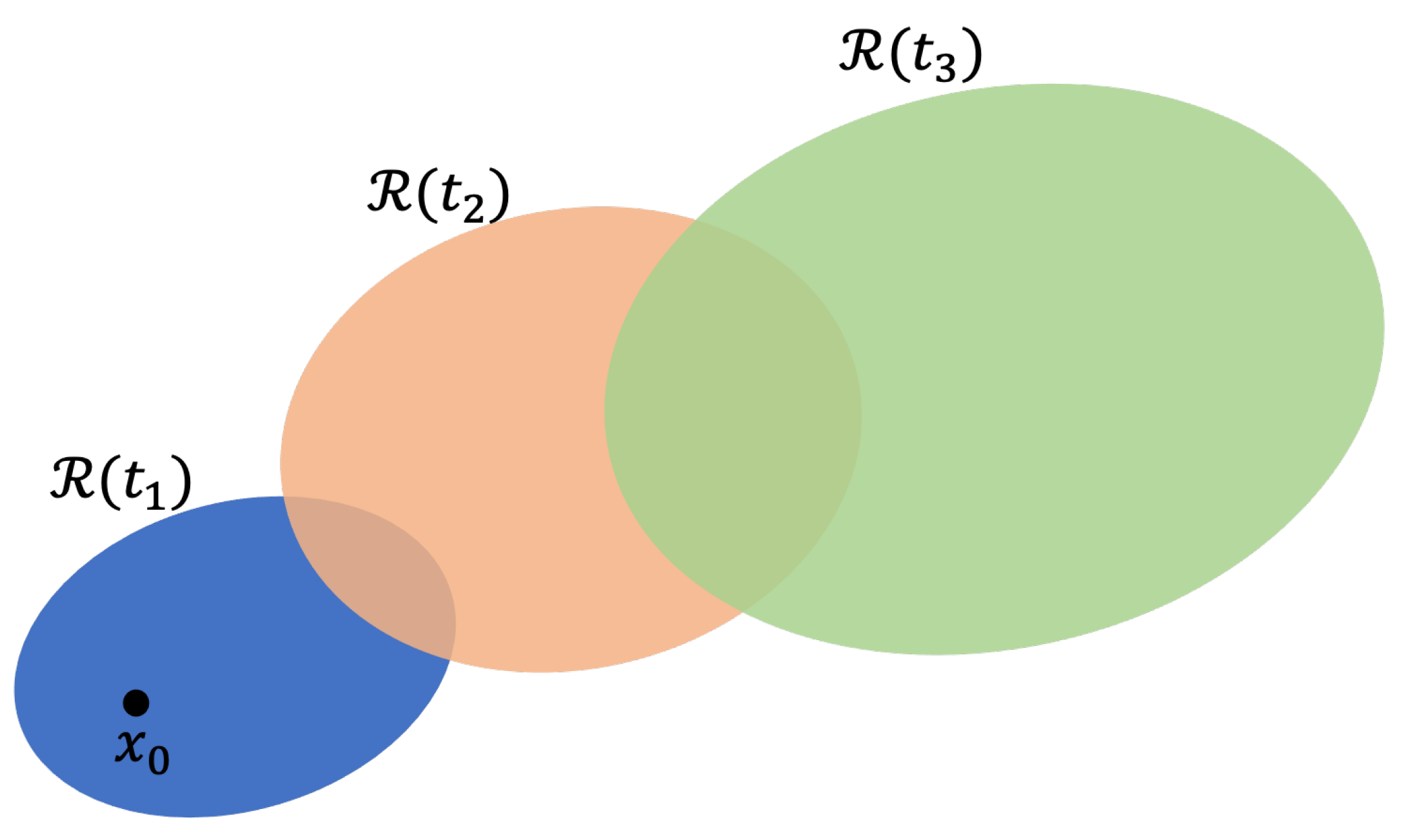
2. Reachable Sets
2.1. Algorithm for Reachable Set Calculation
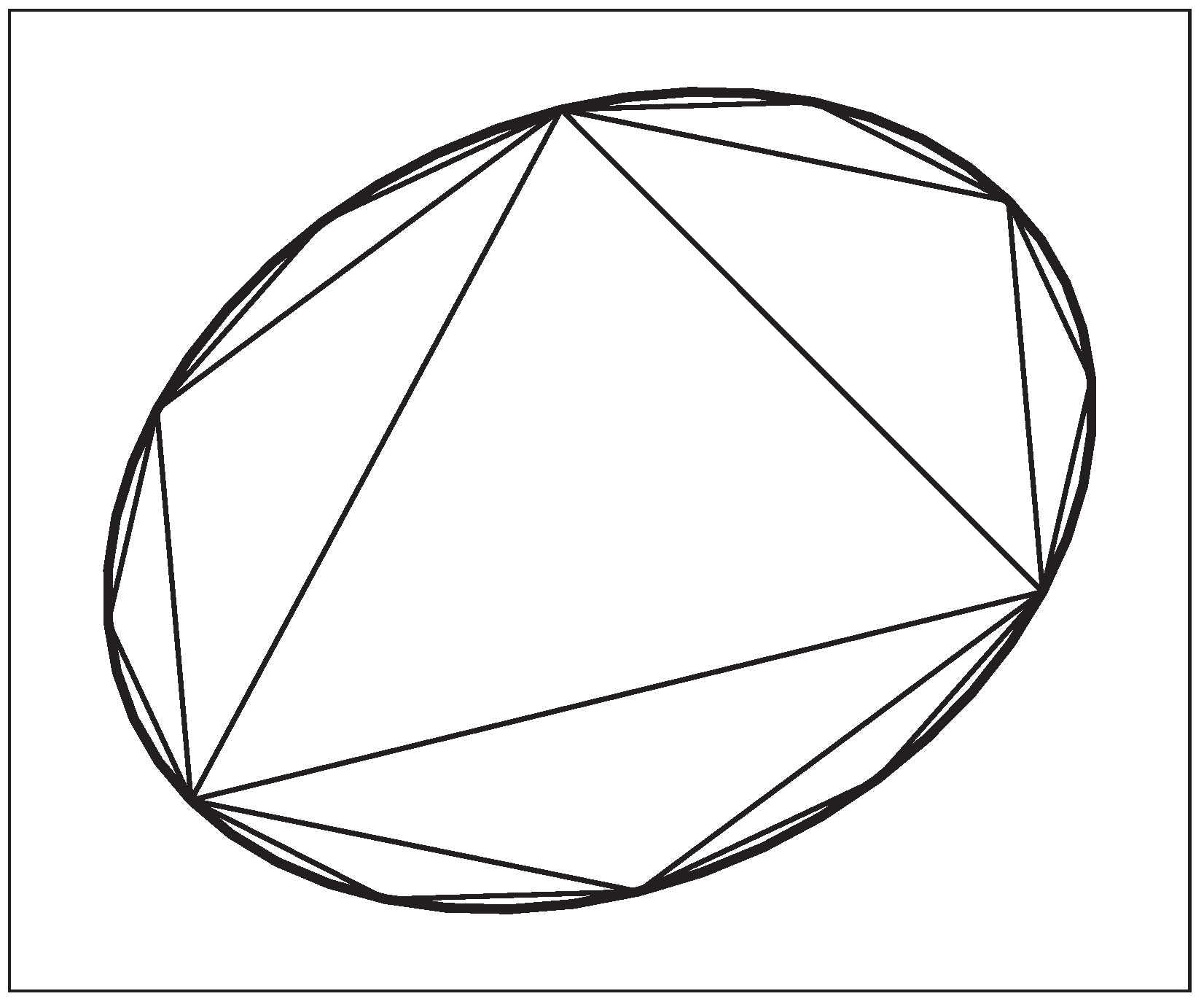
2.1.1. Initial Simplex
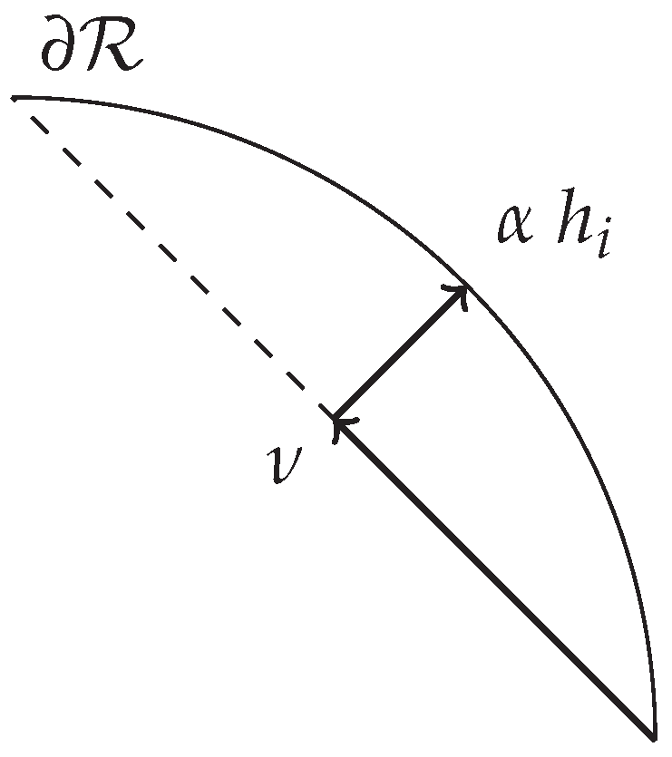
2.1.2. Growing Simplices
3. Game Theory
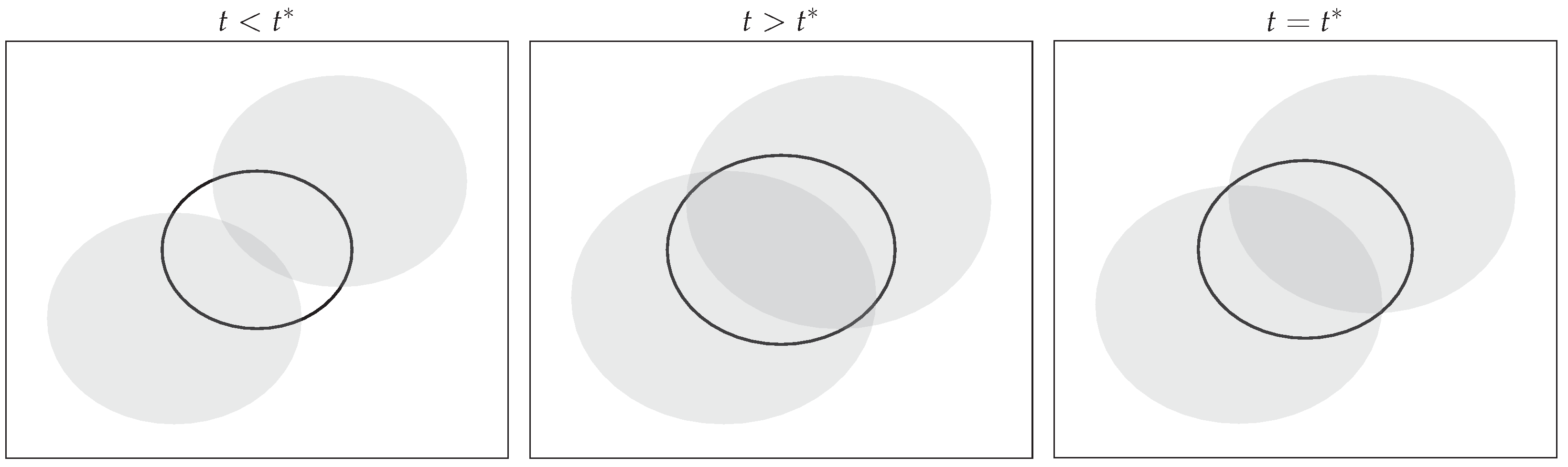
3.1. Single Pursuer and Single Evader
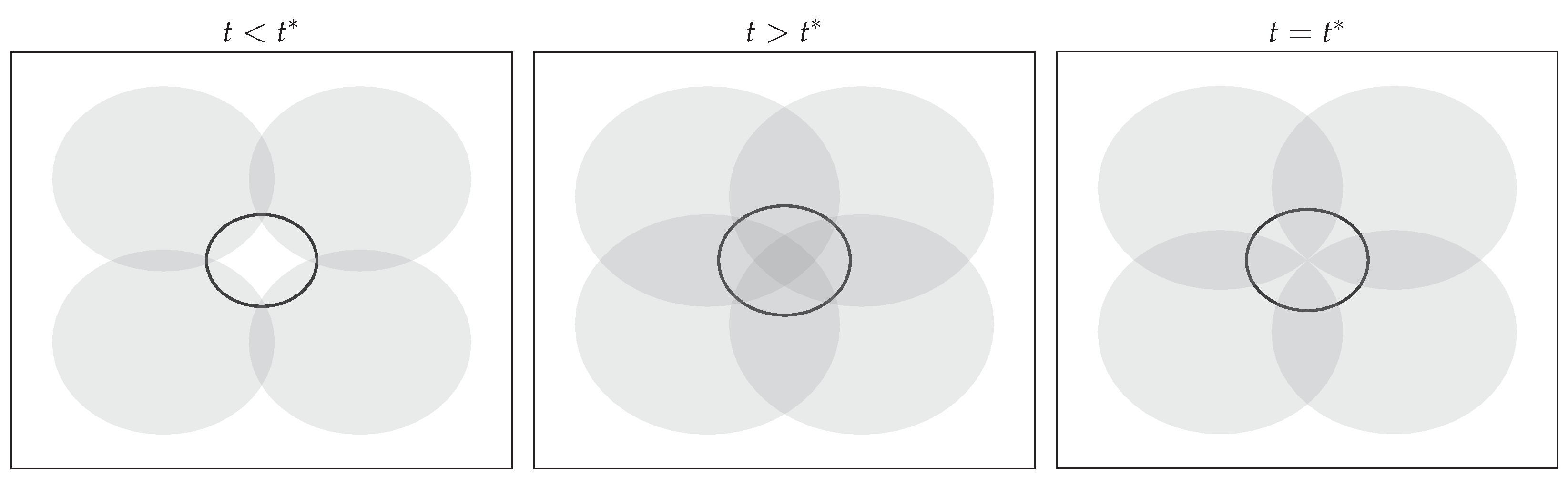
3.2. Multiple Pursuers and Single Evader
| Algorithm 1 Line Search for Capture Time in Multiple Pursuer and Single Evader Game |
|
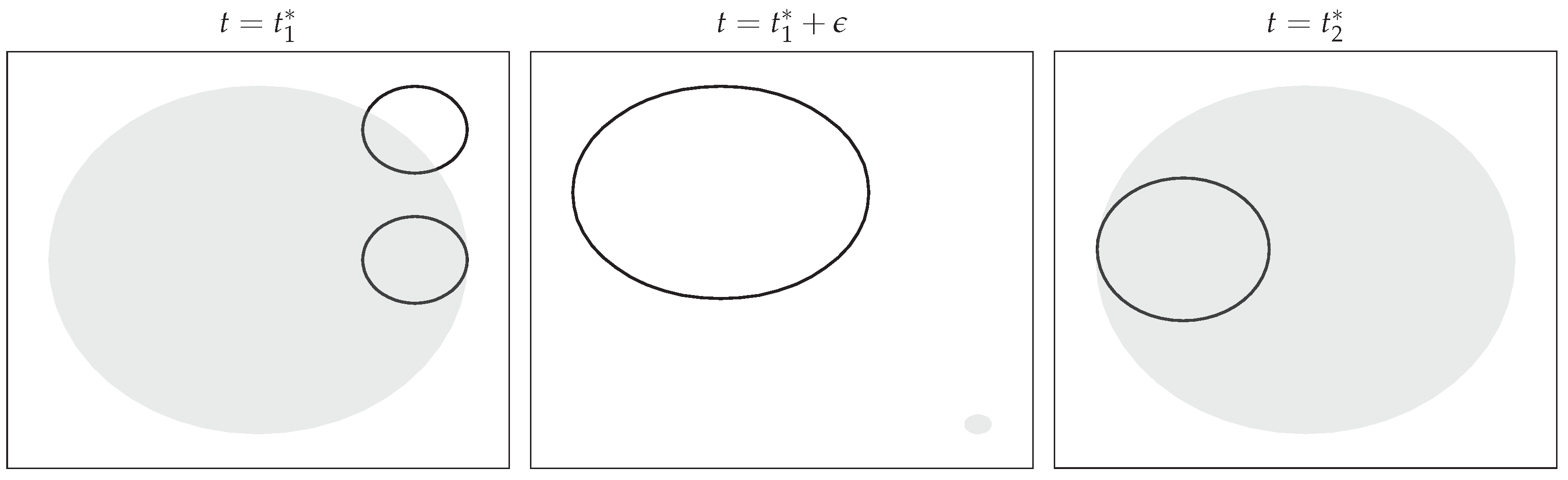
3.3. Single Pursuer and Multiple Evaders
| Algorithm 2 Termination Time in Single Pursuer and Multiple Evader Game |
|
4. Dynamics
5. Numerical Simulations
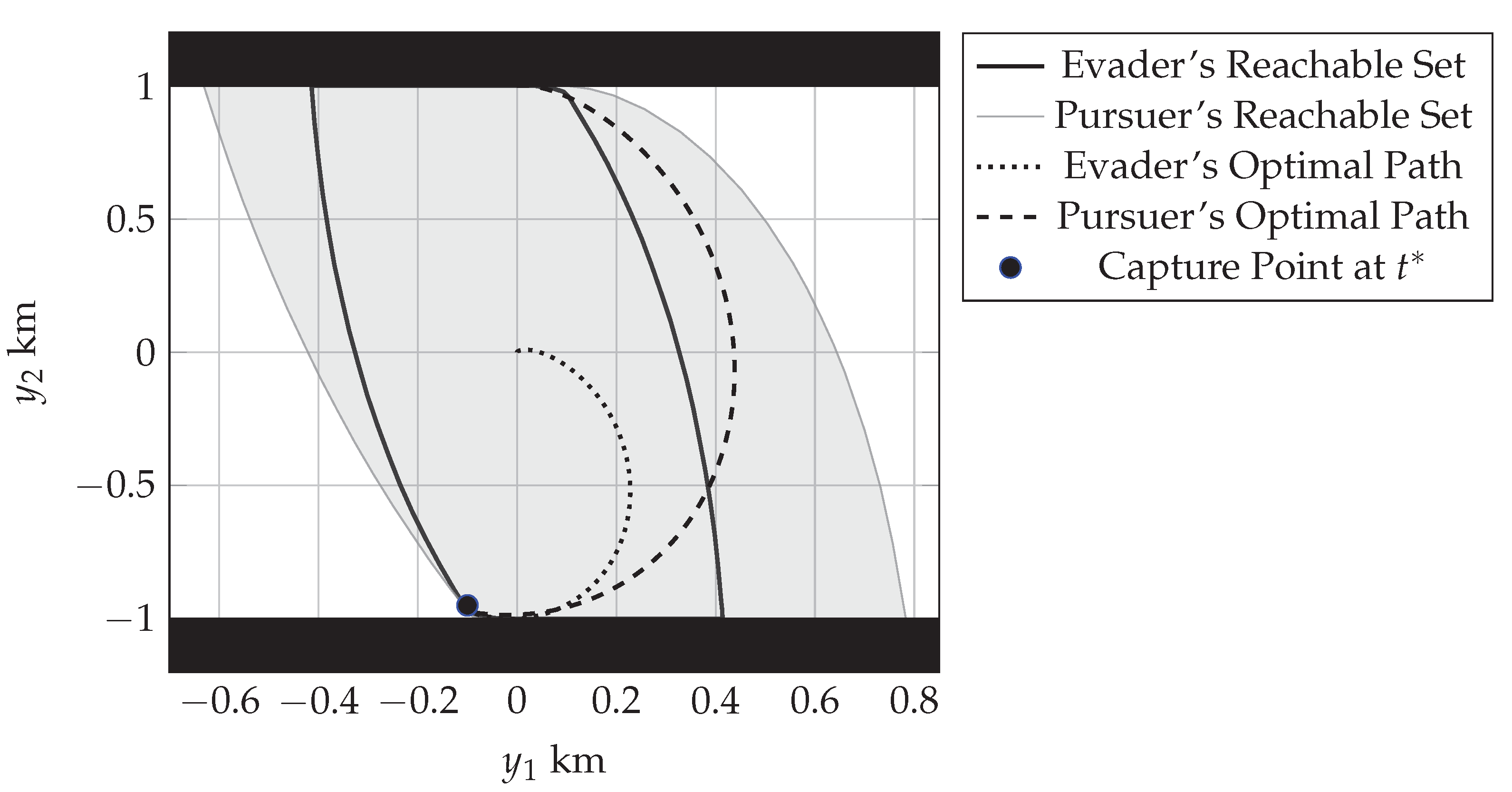
5.1. Single Pursuer and Single Evader
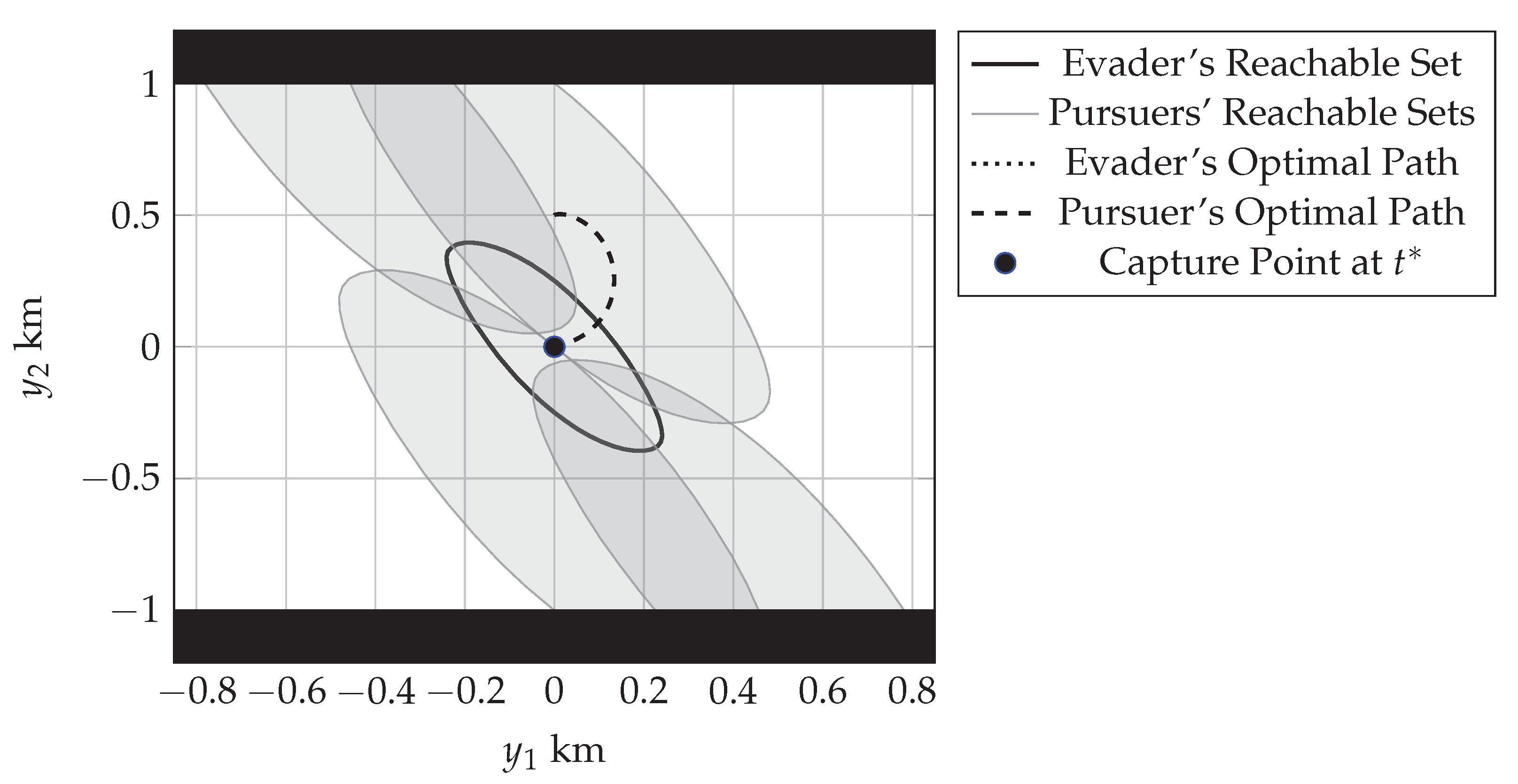
5.2. Multiple Pursuers and Single Evader
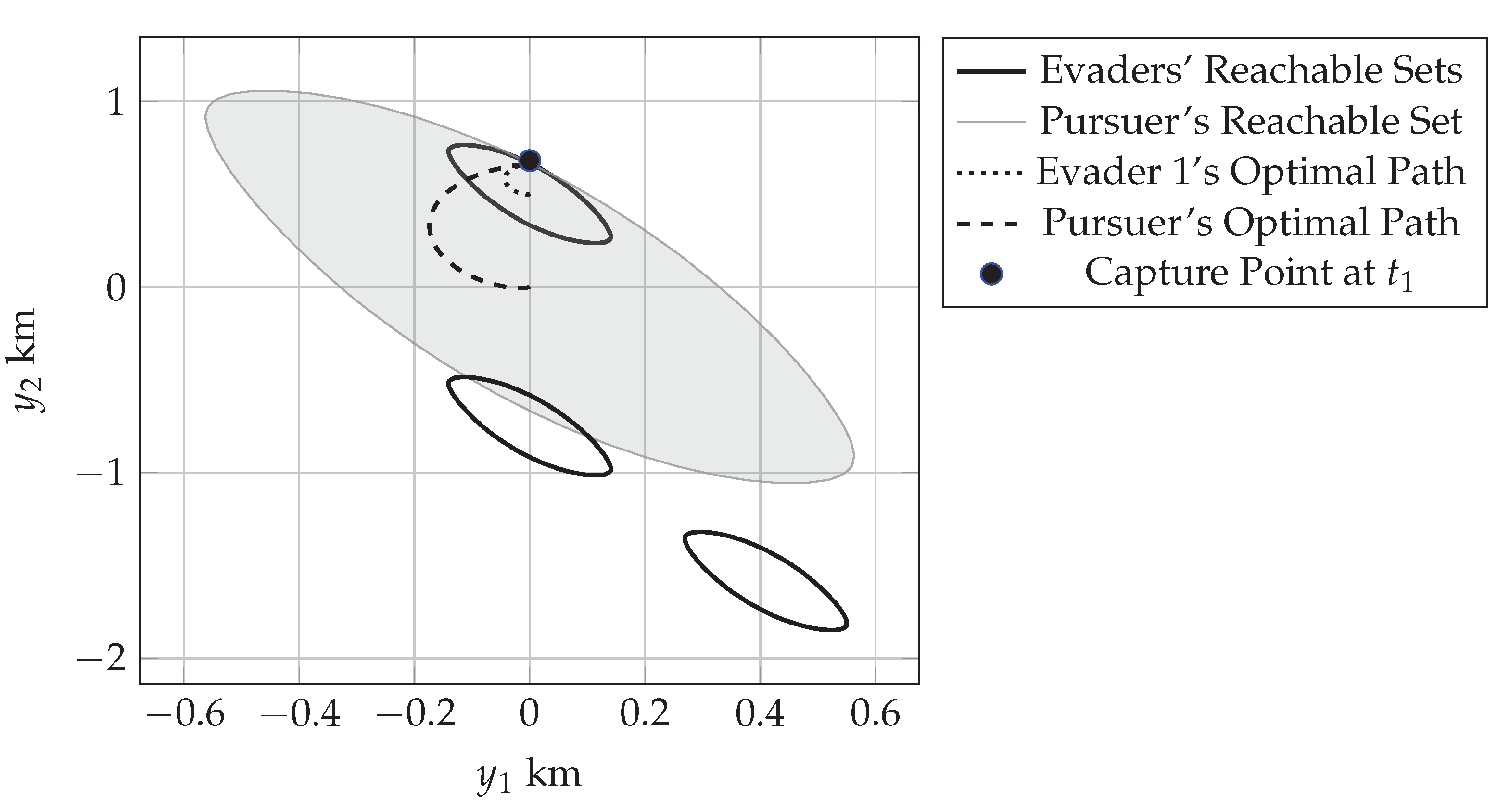
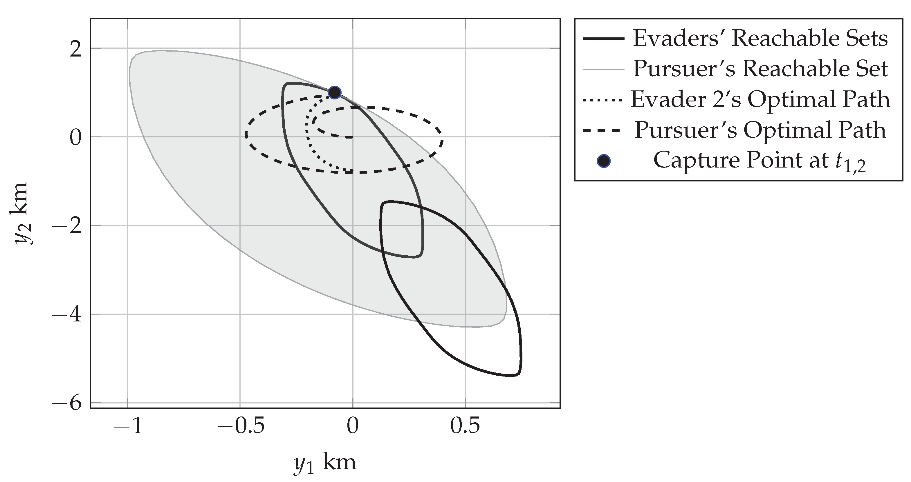
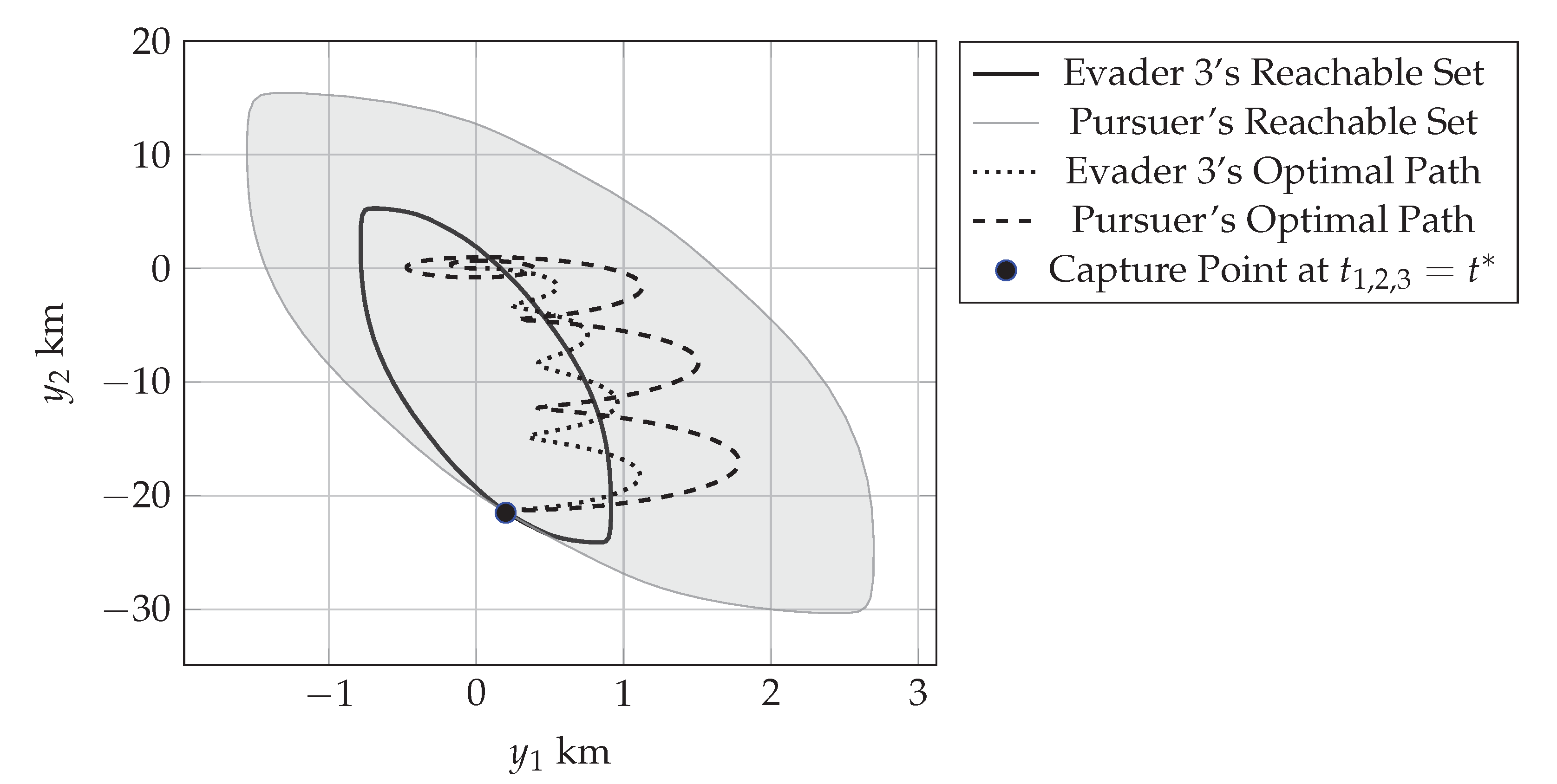
5.3. Single Pursuer and Multiple Evaders
5.4. Computational Performance
6. Conclusions
Author Contributions
Funding
Data Availability Statement
Conflicts of Interest
Appendix A
References
- Mizukami, K.; Eguchi, K. A geometrical approach to problems of pursuit-evasion games. J. Frankl. Inst. 1977, 303, 371–384. [Google Scholar] [CrossRef]
- Isaacs, R. Differential Games: A Mathematical Theory with Applications to Warfare and Pursuit, Control and Optimization; Dover Publications: Mineola, NY, USA, 1999. [Google Scholar]
- Weintraub, I.E.; Pachter, M.; Garcia, E. An introduction to pursuit-evasion differential games. In Proceedings of the 2020 American Control Conference (ACC), IEEE, Denver, CO, USA, 1–3 July 2020; pp. 1049–1066. [Google Scholar]
- Shinar, J.; Gutman, S. Recent advances in optimal pursuit and evasion. In Proceedings of the 1978 IEEE Conference on Decision and Control Including the 17th Symposium on Adaptive Processes, IEEE, San Diego, CA, USA, 10–12 January 1979; pp. 960–965. [Google Scholar]
- Shinar, J.; Glizer, V.Y.; Turetsky, V. A pursuit-evasion game with hybrid pursuer dynamics. Eur. J. Control 2009, 15, 665–684. [Google Scholar] [CrossRef]
- Shinar, J. Solution techniques for realistic pursuit-evasion games. In Control and Dynamic Systems; Elsevier: Amsterdam, The Netherlands, 1981; Volume 17, pp. 63–124. [Google Scholar]
- Imado, F.; Kuroda, T. A method to solve missile-aircraft pursuit-evasion differential games. IFAC Proc. Vol. 2005, 38, 176–181. [Google Scholar] [CrossRef]
- Carr, R.W.; Cobb, R.G.; Pachter, M.; Pierce, S. Solution of a Pursuit–Evasion game using a near-optimal strategy. J. Guid. Control Dyn. 2018, 41, 841–850. [Google Scholar] [CrossRef]
- Greenwood, N. A differential game in three dimensions: The aerial dogfight scenario. Dyn. Control 1992, 2, 161–200. [Google Scholar] [CrossRef]
- Calise, A.J.; Yu, X.m. An analysis of a four state model for pursuit-evasion games. In Proceedings of the 1985 24th IEEE Conference on Decision and Control, IEEE, Fort Lauderdale, FL, USA, 11–13 December 1985; pp. 1119–1121. [Google Scholar]
- Horie, K.; Conway, B.A. Optimal fighter pursuit-evasion maneuvers found via two-sided optimization. J. Guid. Control Dyn. 2006, 29, 105–112. [Google Scholar] [CrossRef]
- Shen, D.; Pham, K.; Blasch, E.; Chen, H.; Chen, G. Pursuit-evasion orbital game for satellite interception and collision avoidance. In Proceedings of the Sensors and Systems for Space Applications IV, International Society for Optics and Photonics, Orlando, FL, USA, 25–29 April 2011; Volume 8044, p. 80440B. [Google Scholar]
- Blasch, E.P.; Pham, K.; Shen, D. Orbital satellite pursuit-evasion game-theoretical control. In Proceedings of the 2012 11th International Conference on Information Science, Signal Processing and their Applications (ISSPA), IEEE, Montreal, QC, Canada, 2–5 July 2012; pp. 1007–1012. [Google Scholar]
- Stupik, J.; Pontani, M.; Conway, B. Optimal pursuit/evasion spacecraft trajectories in the hill reference frame. In Proceedings of the AIAA/AAS Astrodynamics Specialist Conference, Minneapolis, MN, USA, 13–16 August 2012; p. 4882. [Google Scholar]
- Shen, D.; Jia, B.; Chen, G.; Pham, K.; Blasch, E. Game optimal sensor management strategies for tracking elusive space objects. In Proceedings of the 2017 IEEE Aerospace Conference, IEEE, Big Sky, MT, USA, 4–11 March 2017; pp. 1–8. [Google Scholar]
- Zeng, X.; Yang, L.; Zhu, Y.; Yang, F. Comparison of Two Optimal Guidance Methods for the Long-Distance Orbital Pursuit-Evasion Game. IEEE Trans. Aerosp. Electron. Syst. 2020, 57, 521–539. [Google Scholar] [CrossRef]
- Yang, B.; Liu, P.; Feng, J.; Li, S. Two-Stage Pursuit Strategy for Incomplete-Information Impulsive Space Pursuit-Evasion Mission Using Reinforcement Learning. Aerospace 2021, 8, 299. [Google Scholar] [CrossRef]
- Bryson, A.; Ho, Y. Applied Optimal Control: Optimization, Estimation and Control; CRC Press: Boca Raton, FL, USA, 1975. [Google Scholar]
- Basar, T. Relaxation Techniques and asynchronous algorithms for online computation of non-cooperative equilibria. J. Econ. Dyn. Control 1987, 11, 531–549. [Google Scholar] [CrossRef]
- Uryasev, S.; Rubinstein, R. On relaxation algorithms in computation of noncooperative equilibria. IEEE Trans. Autom. Control 1994, 39, 1263–1267. [Google Scholar] [CrossRef]
- Johnson, P.A. Numerical Solution Methods for dIfferential Game Problems. Master’s Thesis, Massachusetts Institute of Technology, Cambridge, MA, USA, 2009. [Google Scholar]
- Horie, K.; Conway, B.A. Genetic algorithm preprocessing for numerical solution of differential games problems. J. Guid. Control Dyn. 2004, 27, 1075–1078. [Google Scholar] [CrossRef]
- Sun, W.; Tsiotras, P.; Lolla, T.; Subramani, D.N.; Lermusiaux, P.F. Multiple-pursuer/one-evader pursuit–evasion game in dynamic flowfields. J. Guid. Control Dyn. 2017, 40, 1627–1637. [Google Scholar] [CrossRef]
- Chung, C.F.; Furukawa, T.; Goktogan, A.H. Coordinated control for capturing a highly maneuverable evader using forward reachable sets. In Proceedings of the 2006 IEEE International Conference on Robotics and Automation, ICRA 2006, IEEE, Orlando, FL, USA, 15–19 May 2006; pp. 1336–1341. [Google Scholar]
- Salmon, D.M.; HElNE, W. Reachable sets analysis-an efficient technique for performing missile/sensor tradeoff studies. AIAA J. 1973, 11, 927–931. [Google Scholar] [CrossRef]
- Chung, C.F.; Furukawa, T. A reachability-based strategy for the time-optimal control of autonomous pursuers. Eng. Optim. 2008, 40, 67–93. [Google Scholar] [CrossRef]
- Zanardi, C.; Hervé, J.Y.; Cohen, P. Escape strategy for a mobile robot under pursuit. In Proceedings of the 1995 IEEE International Conference on Systems, Man and Cybernetics. Intelligent Systems for the 21st Century, IEEE, Vancouver, BC, Canada, 22–25 October 1995; Volume 4, pp. 3304–3309. [Google Scholar]
- Jansson, O.; Harris, M.; Geller, D. A Parallelizable Reachable Set Method for Pursuit-Evasion Games Using Interior-Point Methods. In Proceedings of the 2021 IEEE Aerospace Conference (50100), IEEE, Big Sky, MT, USA, 6–13 March 2021; pp. 1–9. [Google Scholar]
- Gong, H.; Gong, S.; Li, J. Pursuit-Evasion Game for Satellites Based on Continuous Thrust Reachable Domain. IEEE Trans. Aerosp. Electron. Syst. 2020, 56, 4626–4637. [Google Scholar] [CrossRef]
- Colonius, F.; Szolnoki, D. Algorithms for computing reachable sets and control sets. IFAC Proc. Vol. 2001, 34, 723–728. [Google Scholar] [CrossRef]
- Girard, A.; Le Guernic, C.; Maler, O. Efficient computation of reachable sets of linear time-invariant systems with inputs. In Proceedings of the International Workshop on Hybrid Systems: Computation and Control, Santa Barbara, CA, USA, 29–31 March 2006; Springer: Berlin/Heidelberg, Germany, 2006; pp. 257–271. [Google Scholar]
- Varaiya, P. Reach set computation using optimal control. In Verification of Digital and Hybrid Systems; Springer: Berlin/Heidelberg, Germany, 2000; pp. 323–331. [Google Scholar]
- Dueri, D.; Raković, S.V.; Açıkmeşe, B. Consistently improving approximations for constrained controllability and reachability. In Proceedings of the 2016 European Control Conference (ECC), IEEE, Aalborg, Denmark, 29 June–1 July 2016; pp. 1623–1629. [Google Scholar]
- Dueri, D.; Açıkmeşe, B.; Baldwin, M.; Erwin, R.S. Finite-horizon controllability and reachability for deterministic and stochastic linear control systems with convex constraints. In Proceedings of the 2014 American Control Conference, IEEE, Portland, OR, USA, 4–6 June 2014; pp. 5016–5023. [Google Scholar]
- Yang, R.; Liu, X. Reachable set computation of linear systems with nonconvex constraints via convex optimization. Automatica 2022, 146, 110632. [Google Scholar] [CrossRef]
- Pecsvaradi, T.; Narendra, K.S. Reachable sets for linear dynamical systems. Inf. Control 1971, 19, 319–344. [Google Scholar] [CrossRef]
- Hermes, H.; LaSalle, J.P. Functional Analysis and Time Optimal Control; Academic Press Inc.: New York, NY, USA, 1969. [Google Scholar]
- Guenin, B.; Konemann, J.; Tuncel, L. A Gentle Introduction to Optimization; Cambridge University Press: Cambridge, UK, 2014. [Google Scholar]
- Clohessy, W.; Wiltshire, R. Terminal guidance system for satellite rendezvous. J. Aerosp. Sci. 1960, 27, 653–658. [Google Scholar] [CrossRef]
- Bennett, T.; Schaub, H. Continuous-Time Modeling and Control Using Nonsingular Linearized Relative-Orbit Elements. J. Guid. Control Dyn. 2016, 39, 2605–2614. [Google Scholar] [CrossRef]
- Sullivan, J.; Grimberg, S.; D’Amico, S. Comprehensive Survey and Assessment of Spacecraft Relative Motion Dynamics Models. J. Guid. Control Dyn. 2017, 40, 1837–1859. [Google Scholar] [CrossRef]
- Toh, K.C.; Todd, M.J.; Tutuncu, R.H. SDPT3—A Matlab software package for semidefinite programming, Version 1.3. Optim. Methods Softw. 1999, 11, 545–581. [Google Scholar] [CrossRef]
- Gurobi Optimization, LLC. Gurobi Optimizer Reference Manual; Gurobi Optimization, LLC: Houston, TX, USA, 2022. [Google Scholar]
- Löfberg, J. YALMIP: A Toolbox for Modeling and Optimization in MATLAB. In Proceedings of the CACSD Conference, Taipei, Taiwan, 2–4 September 2004. [Google Scholar]
- The Mathworks, Inc. MATLAB 2023; The Mathworks, Inc.: Natick, MA, USA, 2023. [Google Scholar]


| Average | Average | Average | Average | |
|---|---|---|---|---|
| Case | SDP Time (s) | SOCP Time (s) | SOCP Number | Total Time (s) |
| Section 5.1 | 0.59 | 0.0068 | 40 | 0.86 |
| Section 5.2 | 0.49 | 0.0064 | 44 | 0.77 |
| Section 5.3 | 0.34 | 0.0059 | 59 | 0.69 |
| Total Time (s) | Total Time (s) | Total Time (s) | Total Time (s) | |
|---|---|---|---|---|
| Case | for 5 itr | for 10 itr | for 25 itr | for 100 itr |
| Section 5.1 | 8.6 | 17.2 | 43.0 | 172 |
| Section 5.2 | 19.3 | 38.5 | 96.3 | 385 |
| Section 5.3 | 13.8 | 27.6 | 69.0 | 276 |
Disclaimer/Publisher’s Note: The statements, opinions and data contained in all publications are solely those of the individual author(s) and contributor(s) and not of MDPI and/or the editor(s). MDPI and/or the editor(s) disclaim responsibility for any injury to people or property resulting from any ideas, methods, instructions or products referred to in the content. |
© 2023 by the authors. Licensee MDPI, Basel, Switzerland. This article is an open access article distributed under the terms and conditions of the Creative Commons Attribution (CC BY) license (https://creativecommons.org/licenses/by/4.0/).
Share and Cite
Jansson, O.; Harris, M.W. A Geometrical, Reachable Set Approach for Constrained Pursuit–Evasion Games with Multiple Pursuers and Evaders. Aerospace 2023, 10, 477. https://doi.org/10.3390/aerospace10050477
Jansson O, Harris MW. A Geometrical, Reachable Set Approach for Constrained Pursuit–Evasion Games with Multiple Pursuers and Evaders. Aerospace. 2023; 10(5):477. https://doi.org/10.3390/aerospace10050477
Chicago/Turabian StyleJansson, Olli, and Matthew W. Harris. 2023. "A Geometrical, Reachable Set Approach for Constrained Pursuit–Evasion Games with Multiple Pursuers and Evaders" Aerospace 10, no. 5: 477. https://doi.org/10.3390/aerospace10050477