

Sensitivity Analysis of Wing Geometric and Kinematic Parameters for the Aerodynamic Performance of Hovering Flapping Wing

Abstract
:1. Introduction
2. Materials and Methods
2.1. Key Parameters Selection
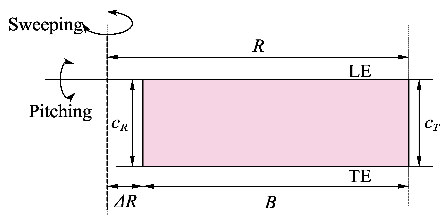
2.2. Wing Geometric Parameters
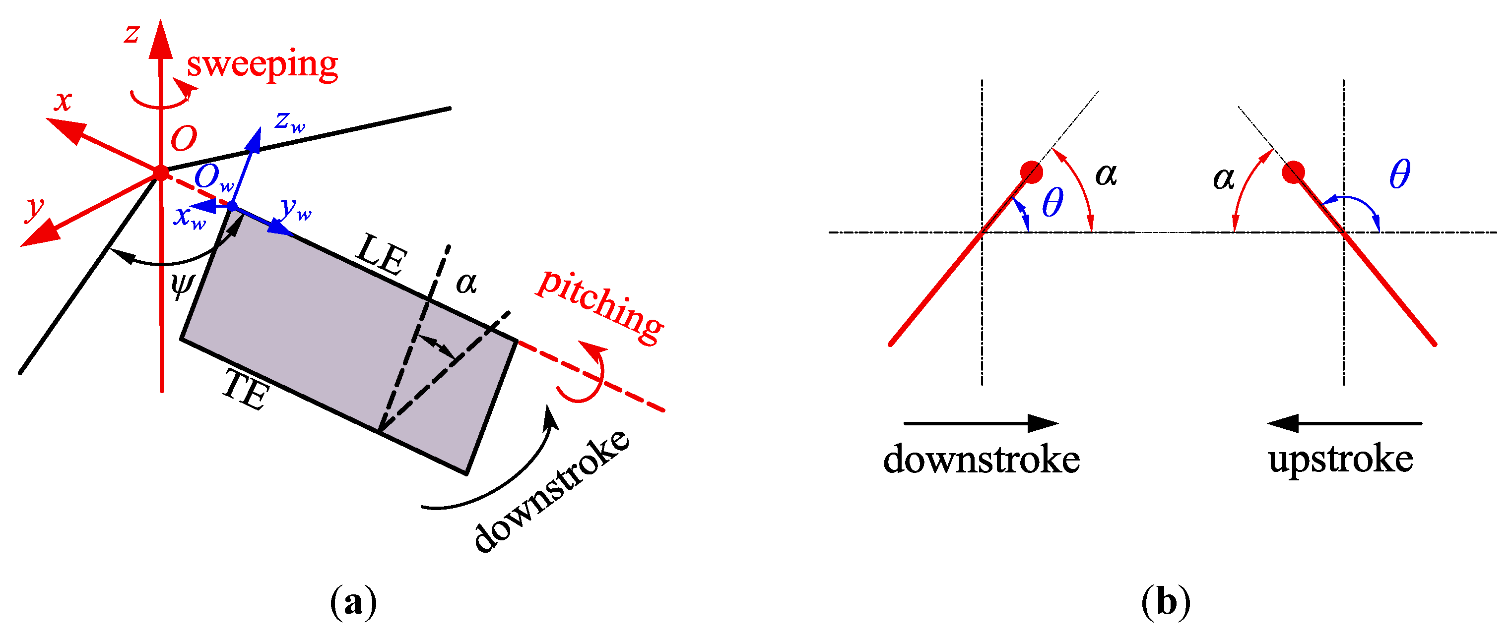
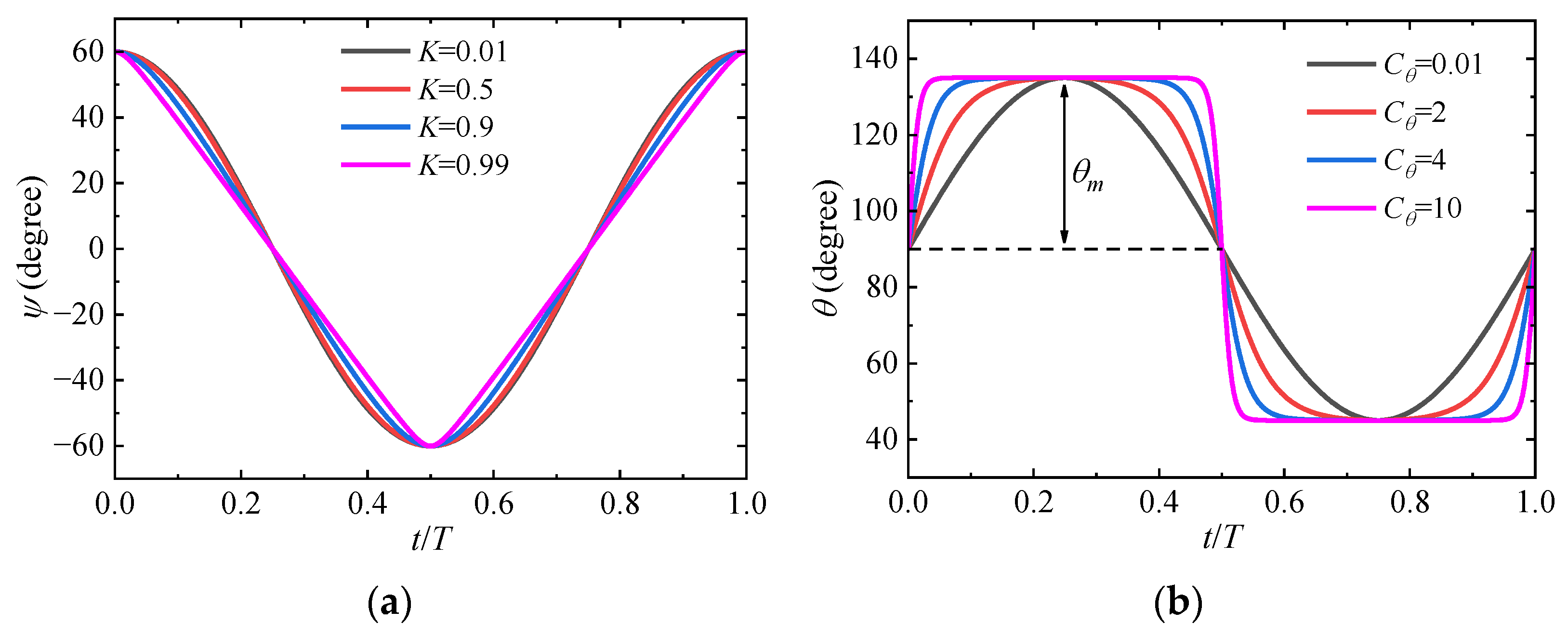
2.3. Wing Kinematic Parameters
2.4. Sensitivity Analysis of Parameters
2.5. Aerodynamic Model, Force and Power Calculation
3. Results and Discussion
3.1. Effect of Wing Geometric Parameters
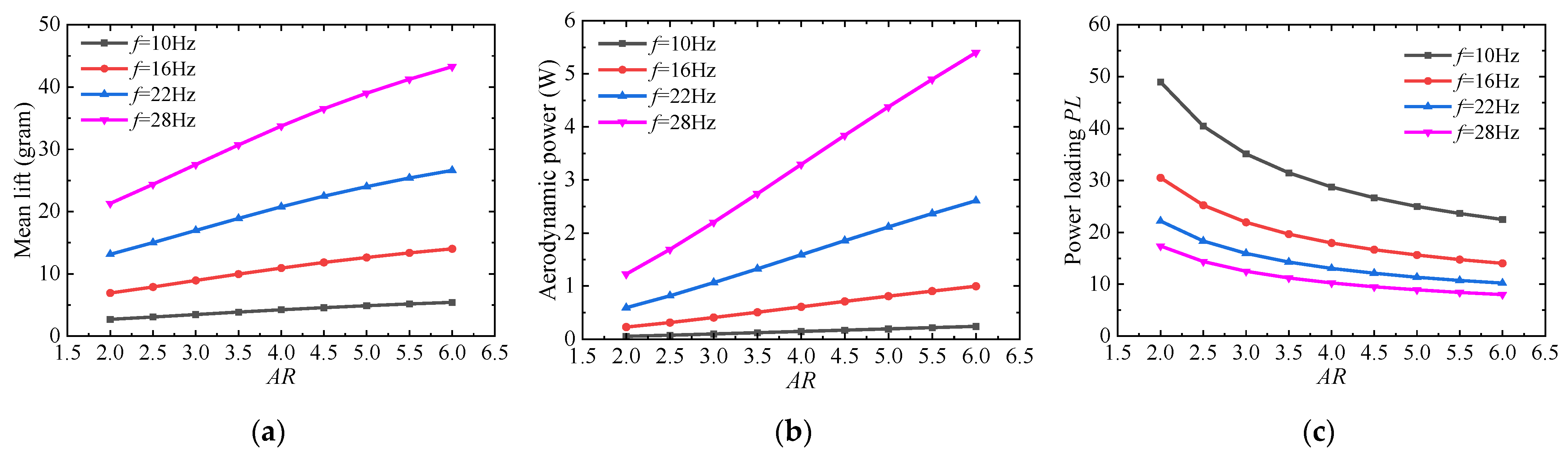
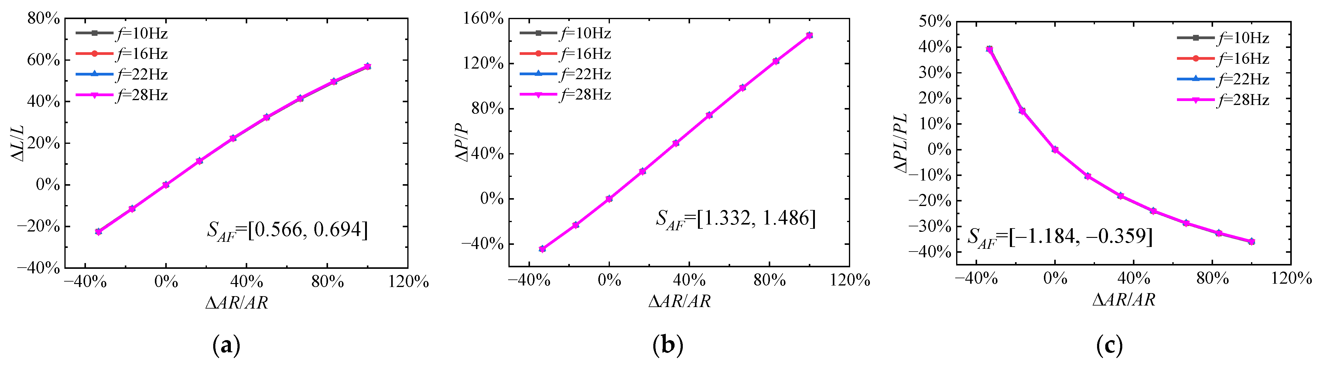
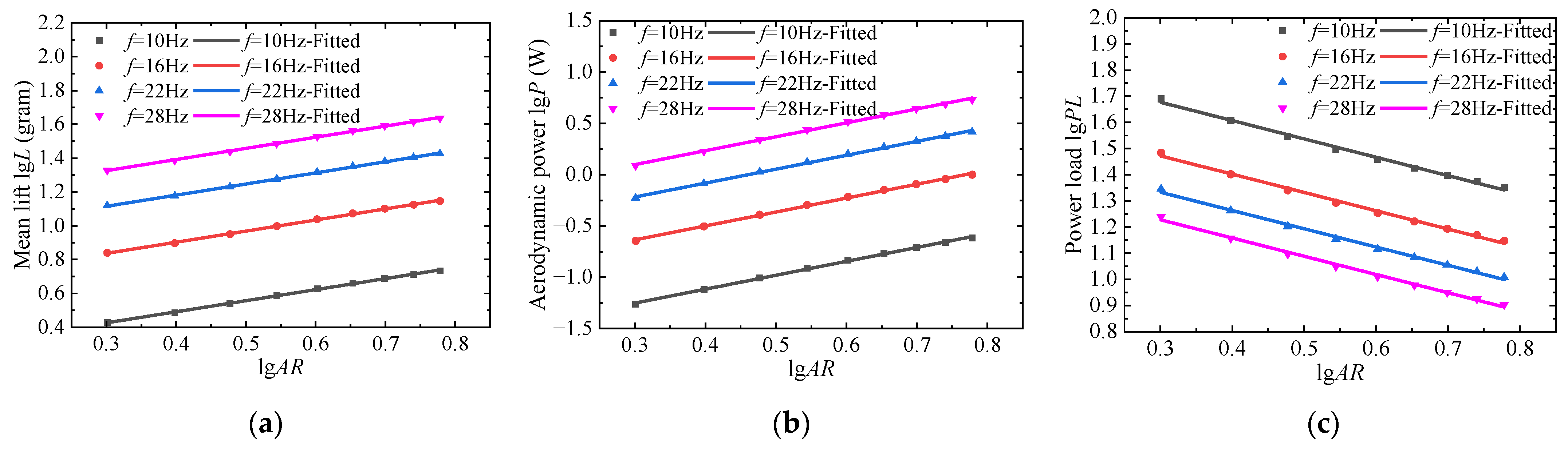
3.1.1. Aspect Ratio AR
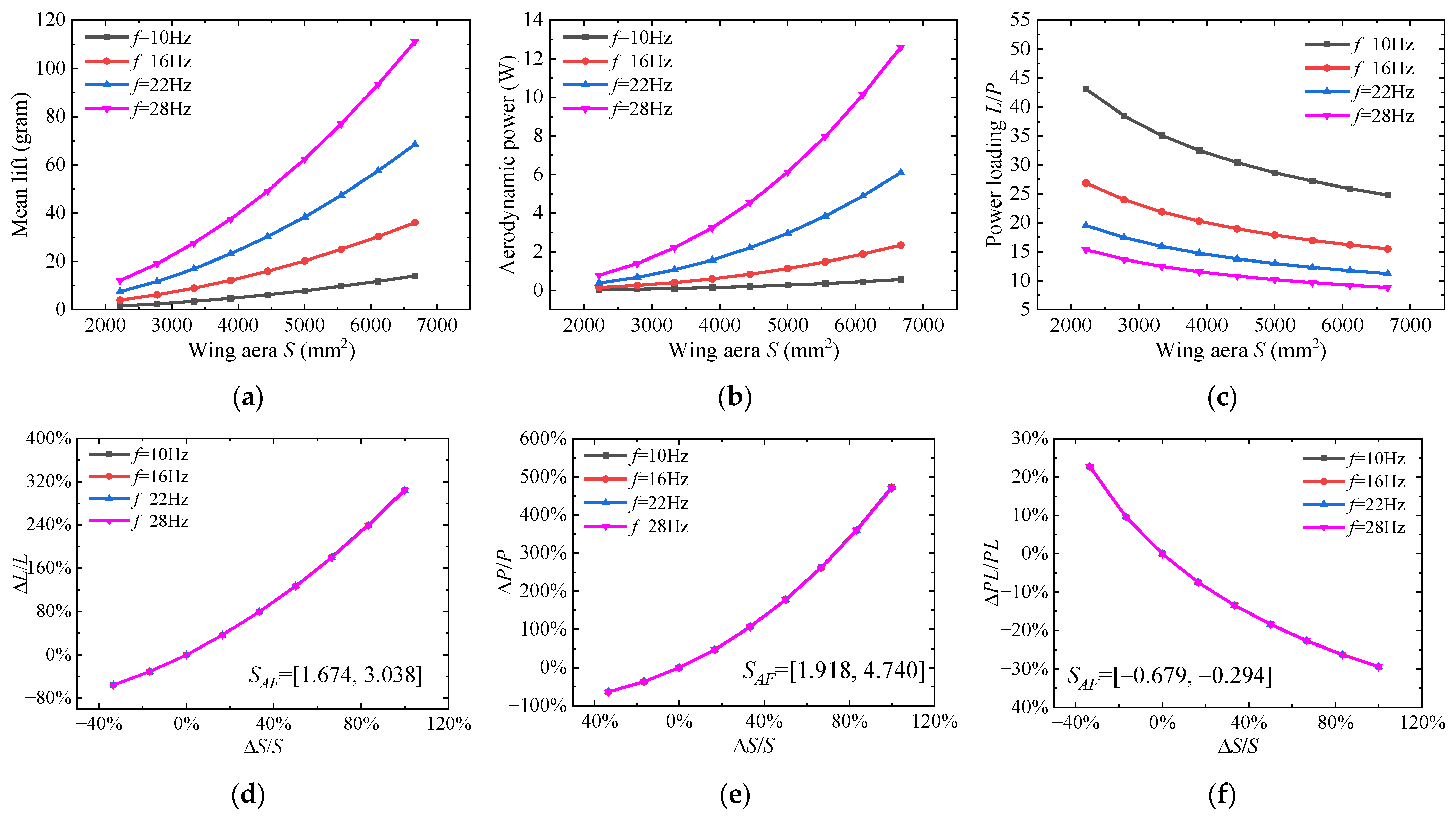
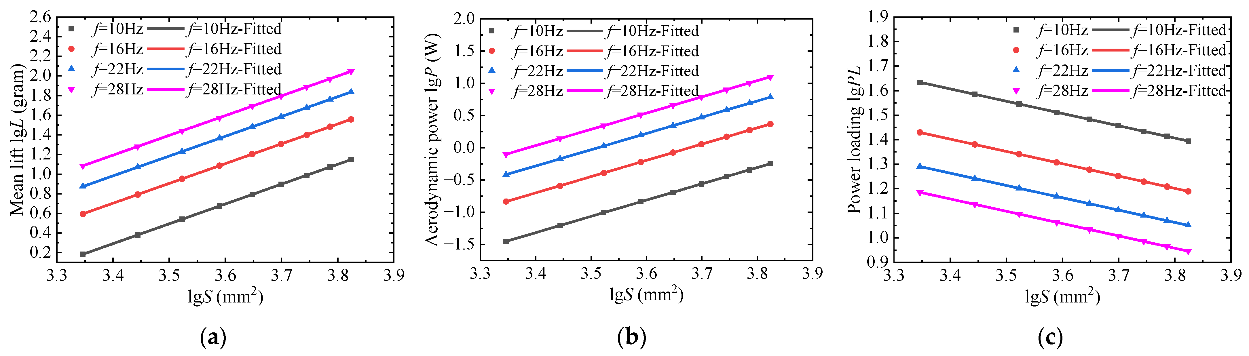
3.1.2. Wing Area S
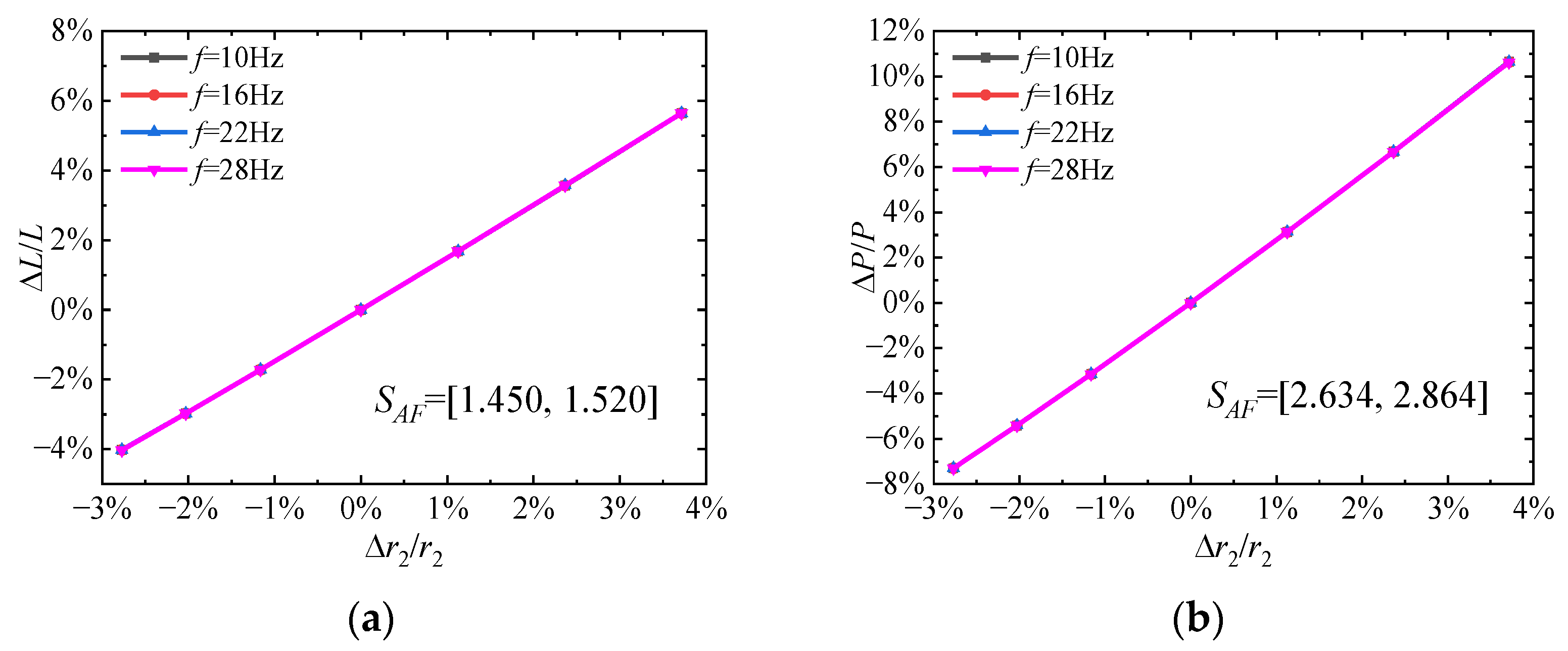
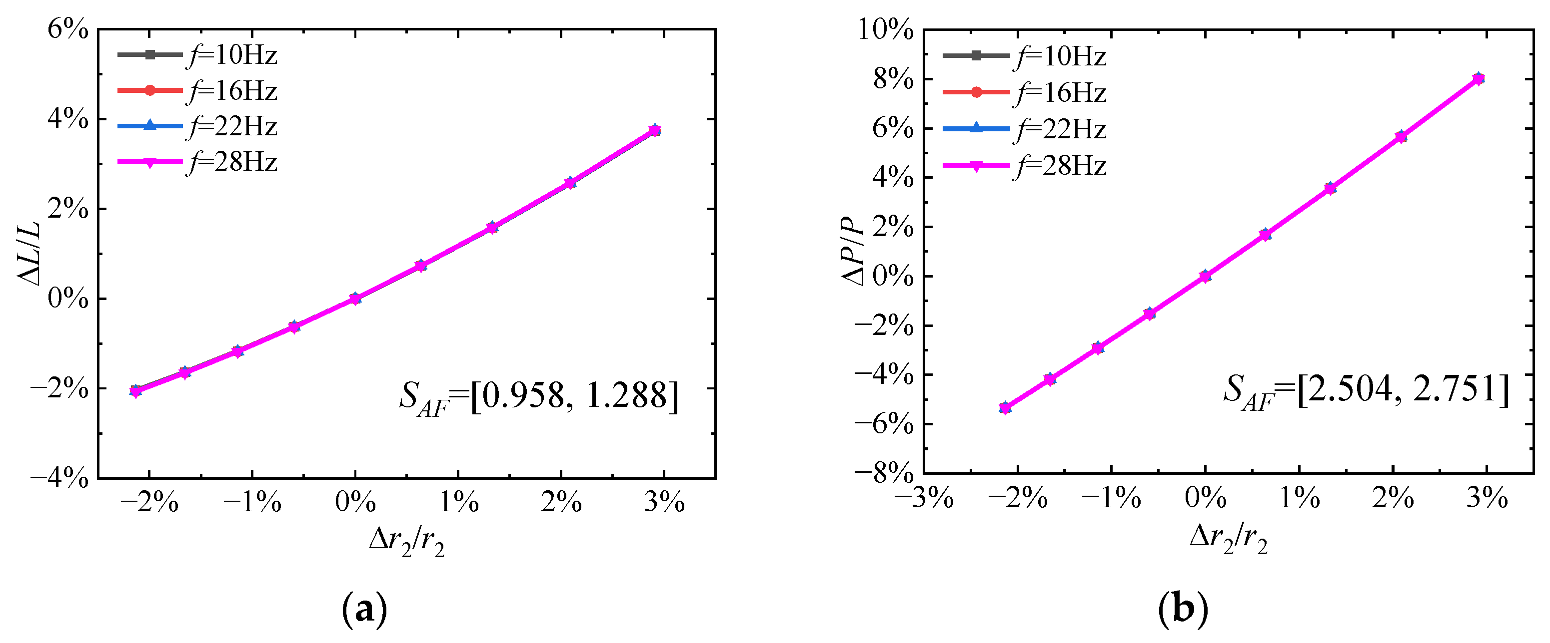
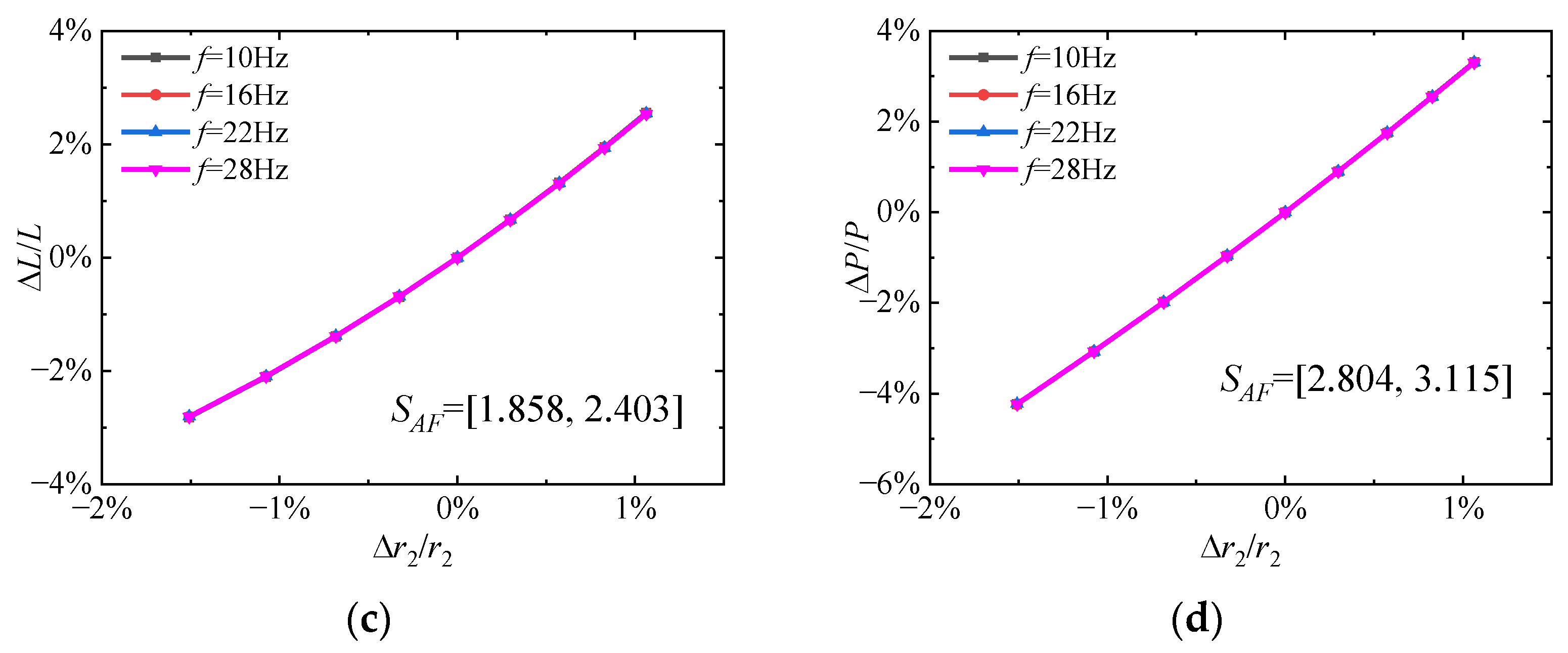
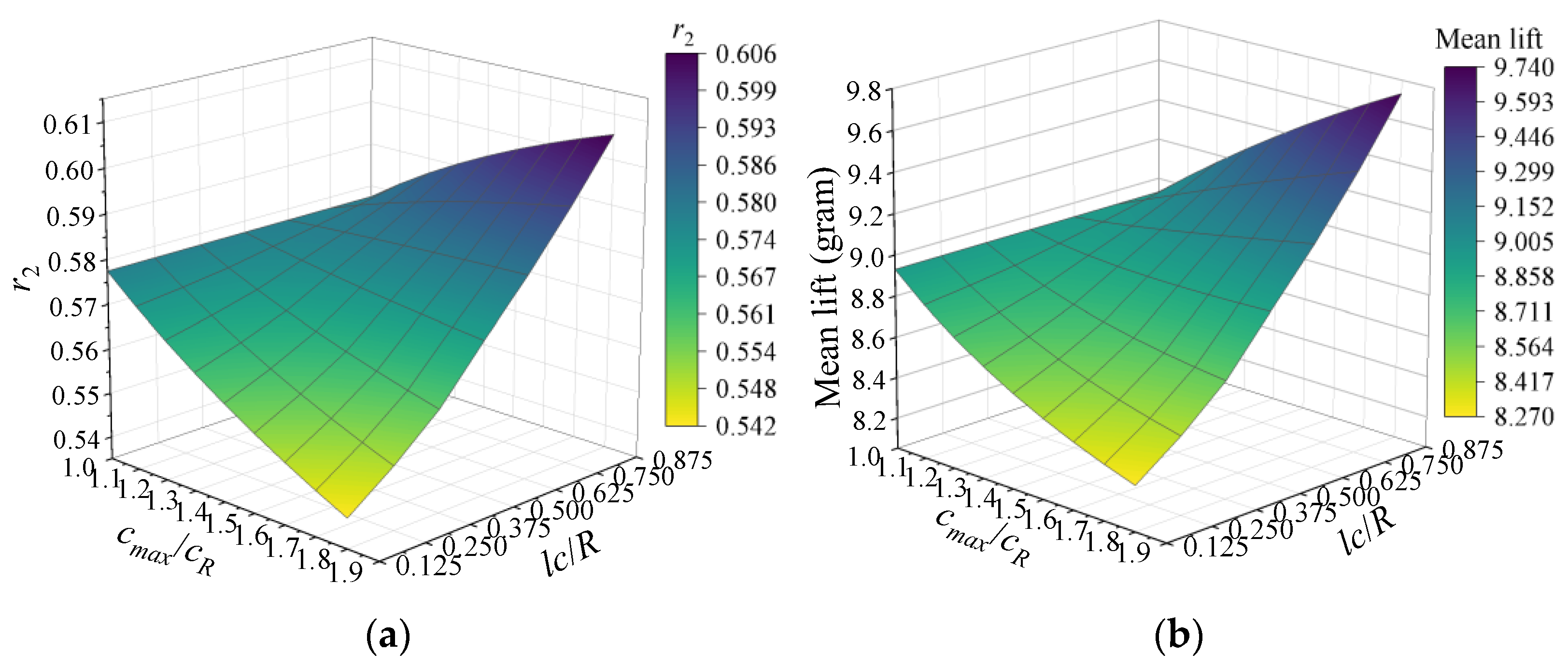
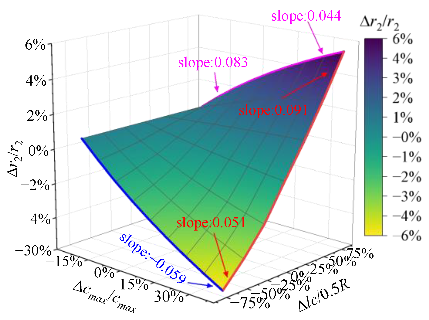
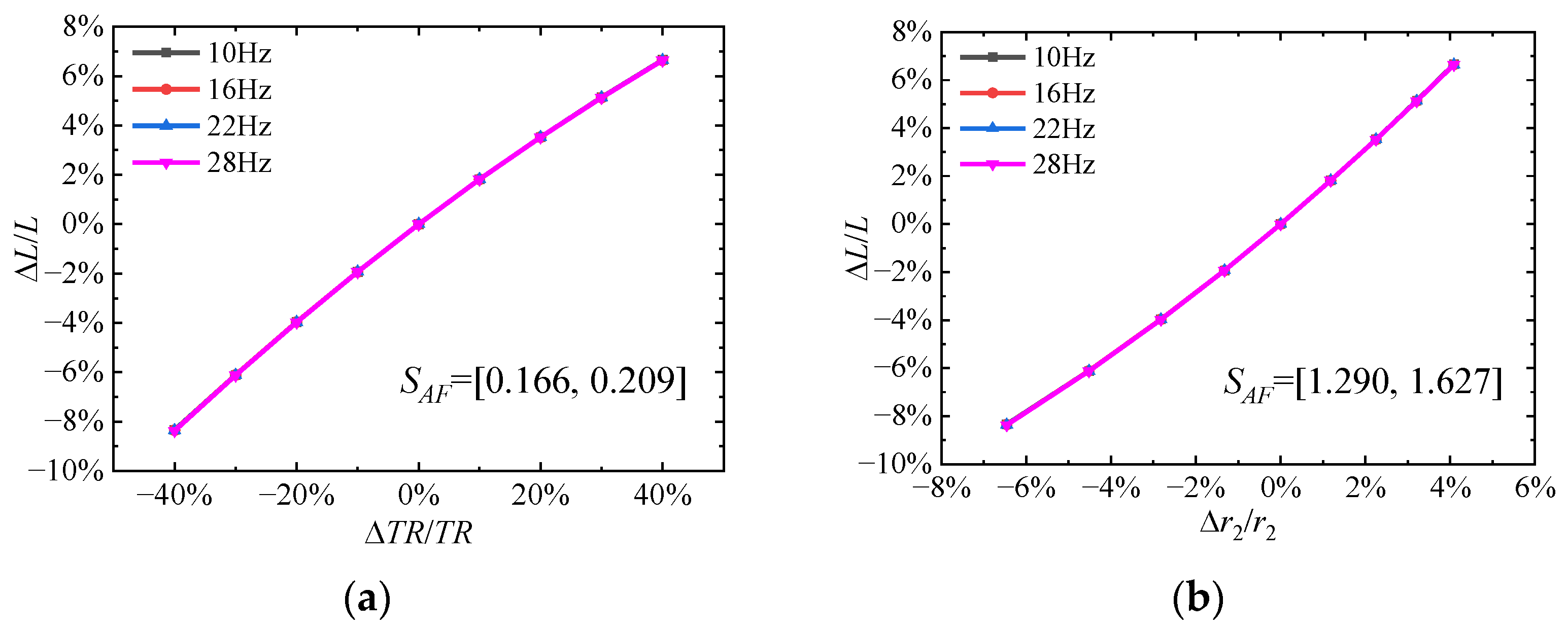
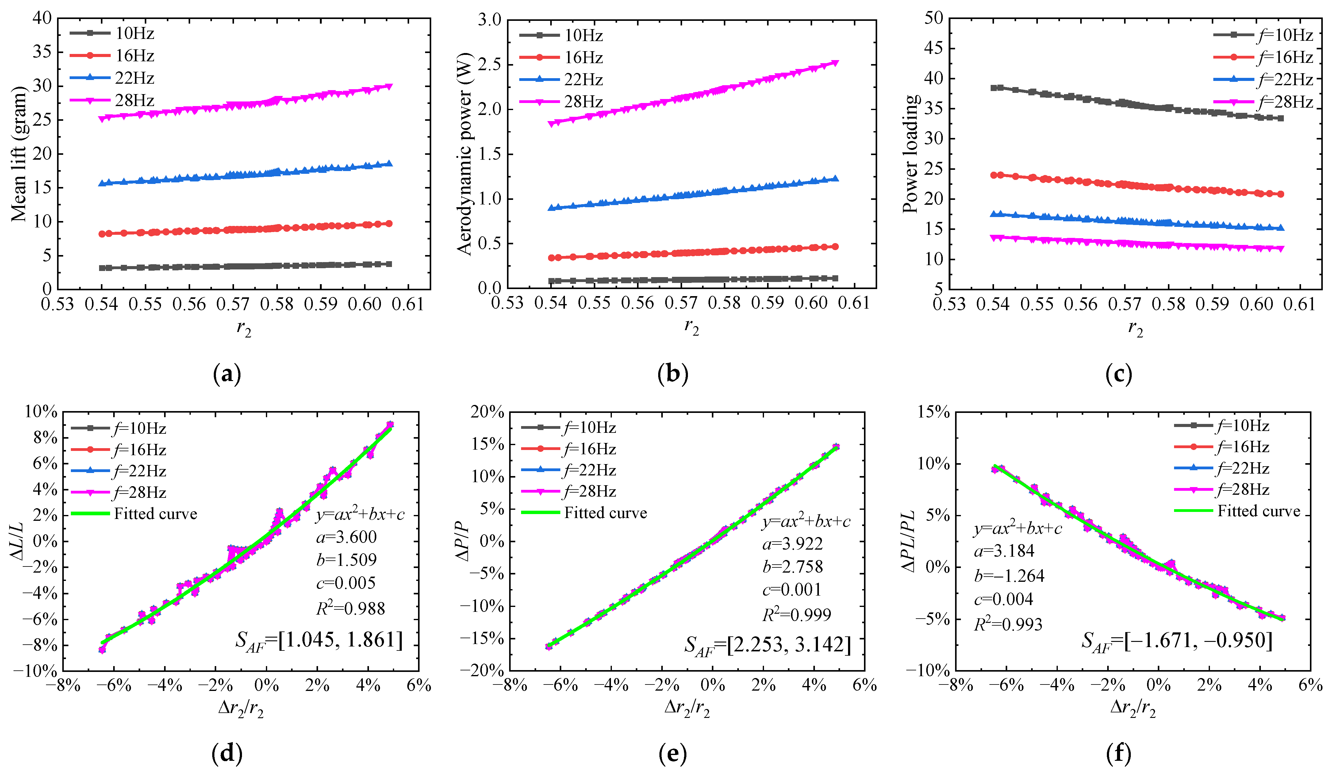
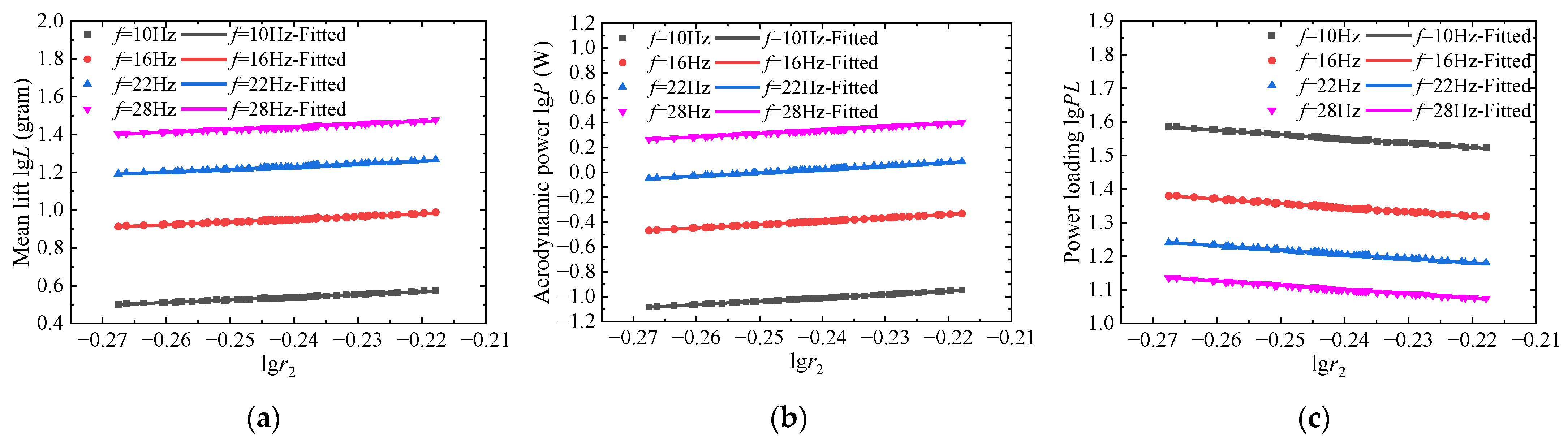
3.1.3. The Dimensionless Radius of the Second Moment of Area r2
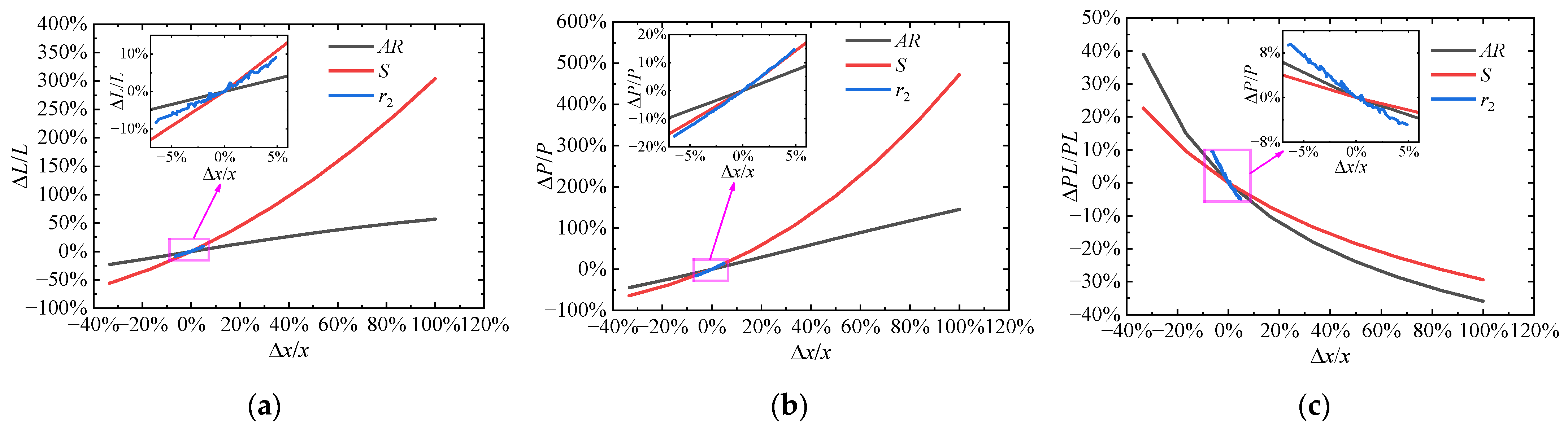
3.1.4. Summary of the Sensitivity Analysis for Wing Geometric Parameters
3.2. Effect of Wing Kinematic Parameters
3.2.1. Flapping Frequency and Sweeping Amplitude
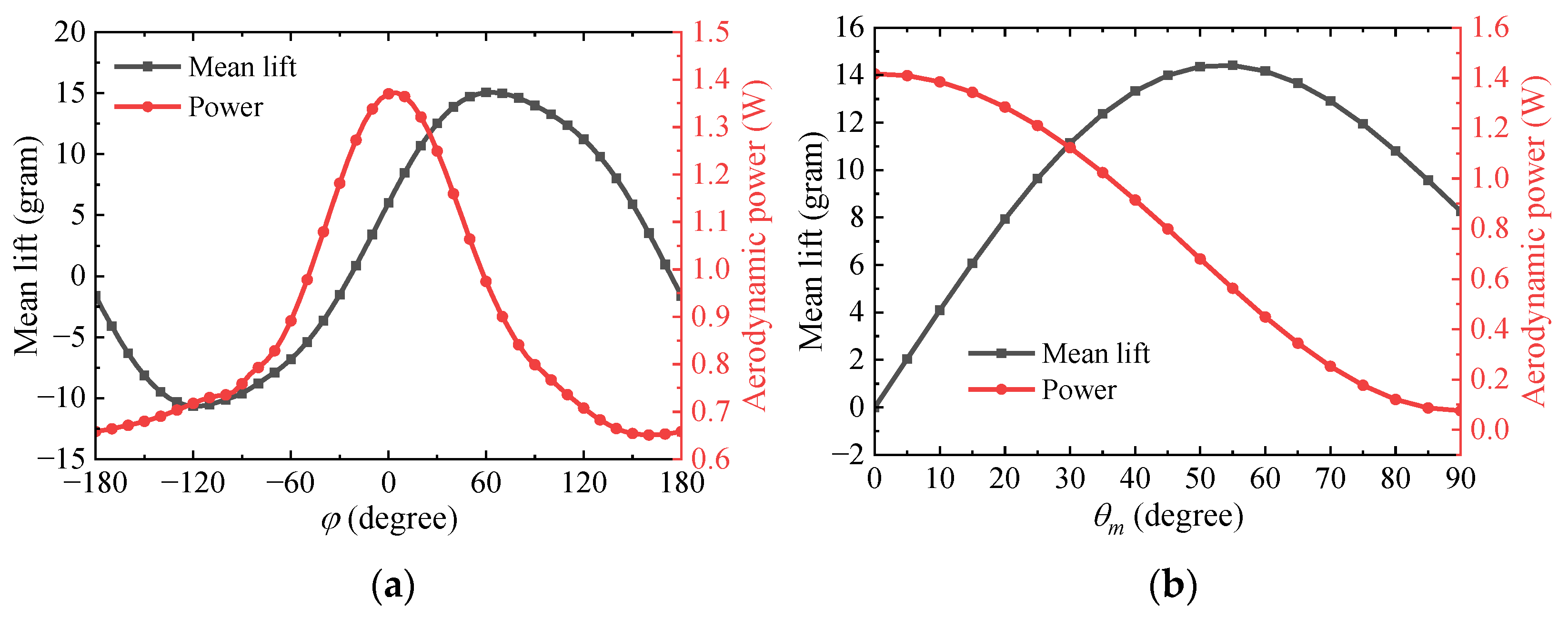
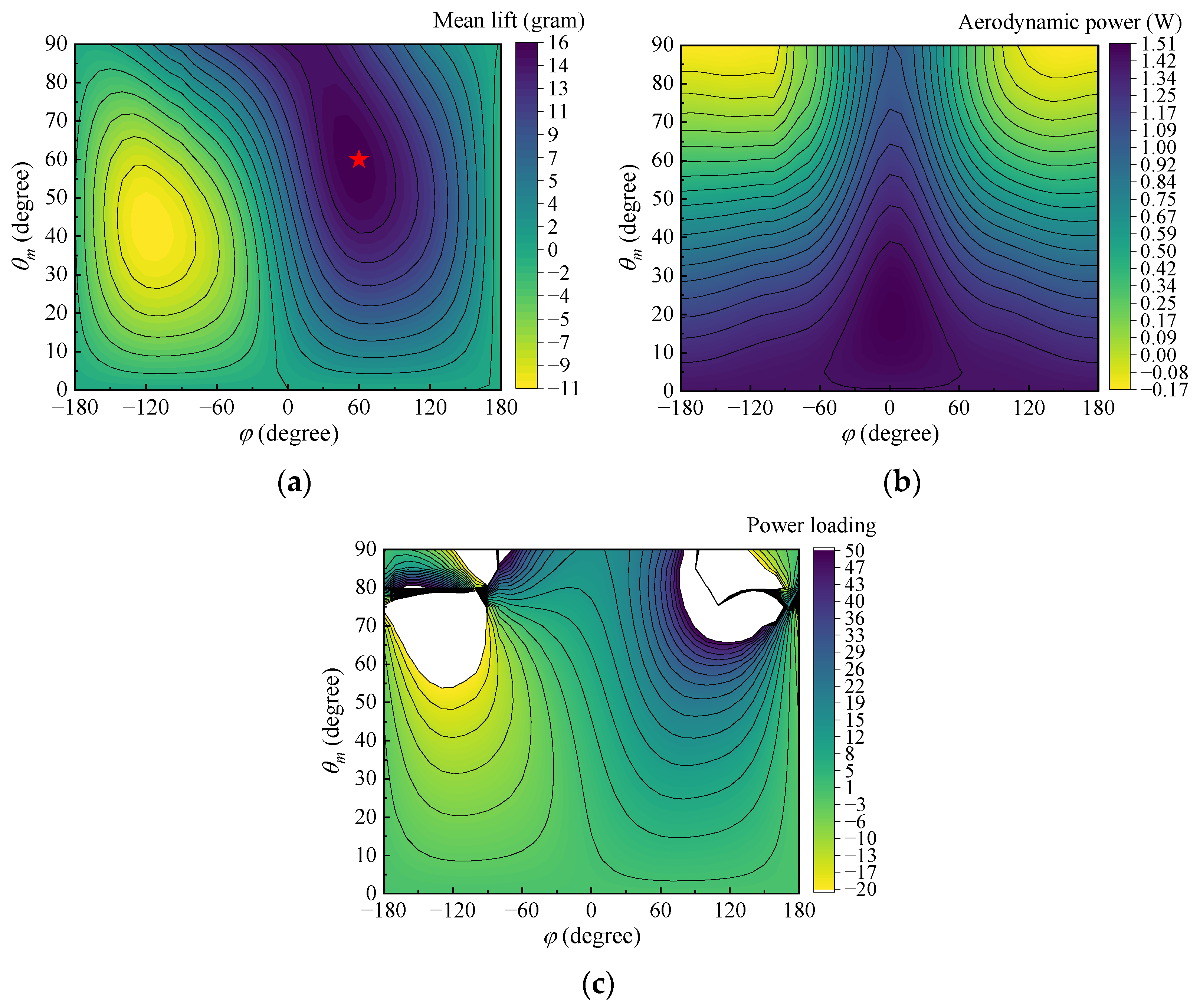
3.2.2. Pitching Amplitude and Phase Shift
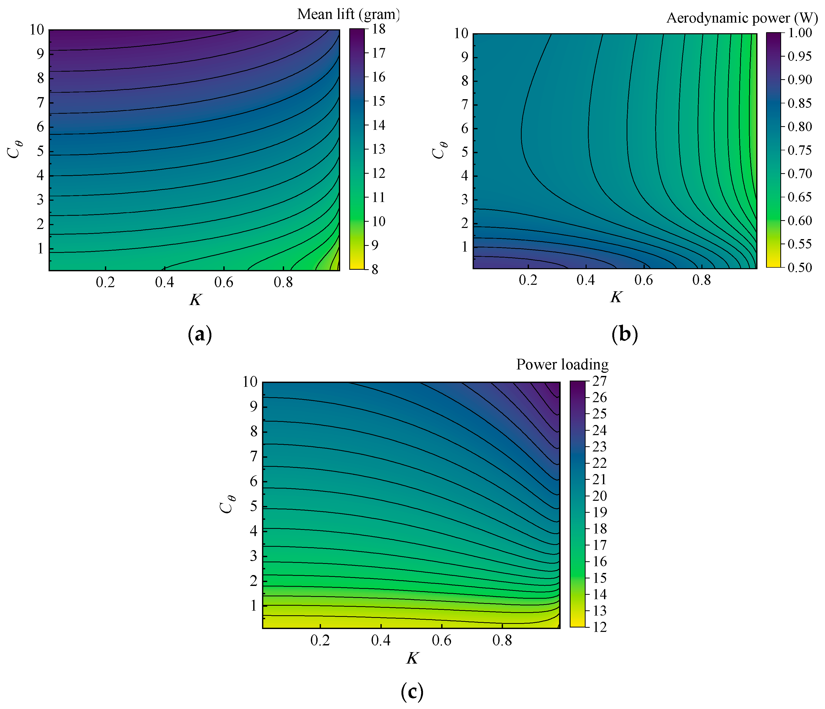
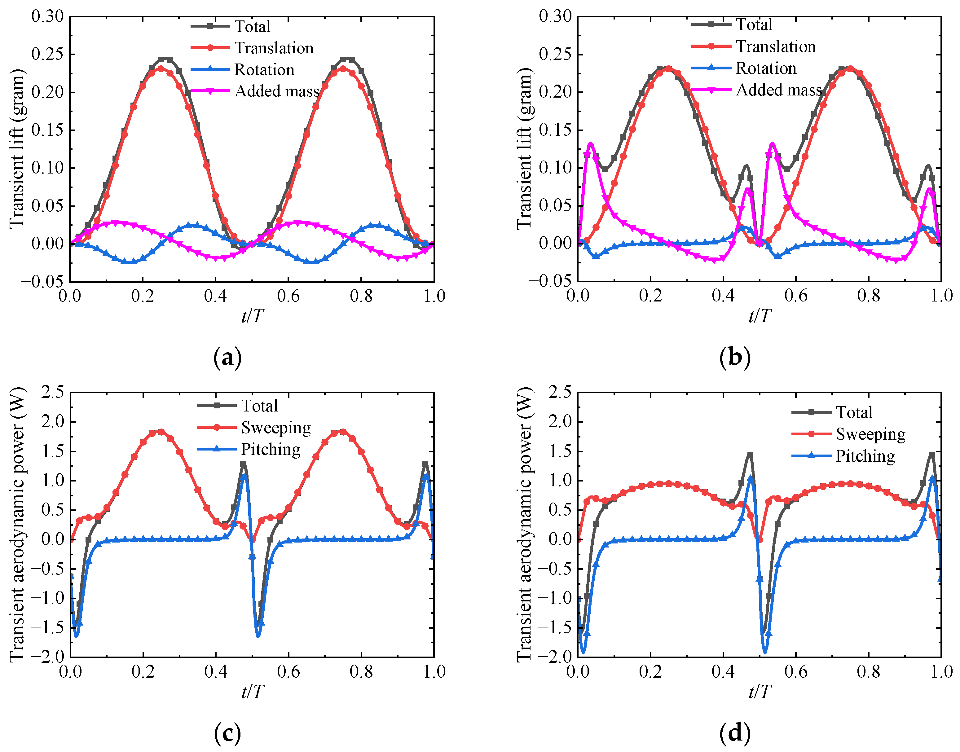
3.2.3. K and Cθ
4. Conclusions
Author Contributions
Funding
Institutional Review Board Statement
Informed Consent Statement
Data Availability Statement
Conflicts of Interest
References
- Xiao, S.J.; Hu, K.; Huang, B.X.; Deng, H.C.; Ding, X.L. A review of research on the mechanical design of hoverable flapping wing micro-air vehicles. J. Bionic Eng. 2021, 18, 1235–1254. [Google Scholar] [CrossRef]
- Phan, H.V.; Park, H.C. Insect-inspired, tailless, hover-capable flapping-wing robots: Recent progress, challenges, and future directions. Prog. Aerosp. Sci. 2019, 111, 100573. [Google Scholar] [CrossRef]
- Keennon, M.; Klingebiel, K.; Won, H.; Andriukov, A. Development of the Nano Hummingbird: A Tailless Flapping Wing Micro Air Vehicle. In Proceedings of the 50th AIAA Aerospace Sciences Meeting including the New Horizons Forum and Aerospace Exposition, Nashville, TN, USA, 9–12 January 2012; p. 0588. [Google Scholar]
- Phan, H.V.; Kang, T.; Park, H.C. Design and stable flight of a 21 g insect-like tailless flapping wing micro air vehicle with angular rates feedback control. Bioinspiration Biomim. 2017, 12, 036006. [Google Scholar] [CrossRef] [PubMed]
- Roshanbin, A.; Altartouri, H.; Karásek, M.; Preumont, A. COLIBRI: A hovering flapping twin-wing robot. Int. J. Micro Air Veh. 2017, 9, 270–282. [Google Scholar] [CrossRef] [Green Version]
- Lee, J.; Yoon, S.H.; Kim, C. Experimental surrogate-based design optimization of wing geometry and structure for flapping wing micro air vehicles. Aerosp. Sci. Technol. 2022, 123, 107451. [Google Scholar] [CrossRef]
- Lang, X.Y.; Song, B.F.; Yang, W.Q.; Yang, X.J. Effect of Wing Membrane Material on the Aerodynamic Performance of Flexible Flapping Wing. Appl. Sci. 2022, 12, 4501. [Google Scholar] [CrossRef]
- Tay, W.B.; Jadhav, S.; Wang, J.L. Application and improvements of the wing deformation capture with simulation for flapping micro aerial vehicle. J. Bionic Eng. 2020, 17, 1096–1108. [Google Scholar] [CrossRef]
- Nan, Y.; Karásek, M.; Lalami, M.E.; Preumont, A. Experimental optimization of wing shape for a hummingbird-like flapping wing micro air vehicle. Bioinspiration Biomim. 2017, 12, 026010. [Google Scholar] [CrossRef]
- Ellington, C.P. The aerodynamics of hovering insect flight. VI. Lift and power requirements. Philos. Trans. R. Soc. London. B Biol. Sci. 1984, 305, 145–181. [Google Scholar]
- Shahzad, A.; Tian, F.B.; Young, J.; Lai, J.C. Effects of wing shape, aspect ratio and deviation angle on aerodynamic performance of flapping wings in hover. Phys. Fluids 2016, 28, 111901. [Google Scholar] [CrossRef]
- Hassanalian, M.; Throneberry, G.; Abdelkefi, A. Investigation on the planform and kinematic optimization of bio-inspired nano air vehicles for hovering applications. Meccanica 2018, 53, 2273–2286. [Google Scholar] [CrossRef]
- Broadley, P.A.; Nabawy, M.R.; Quinn, M.K.; Crowther, W.J. Wing planform effects on the aerodynamic performance of insect-like revolving wings. In Proceedings of the AIAA Aviation 2020 Forum, Virtual, 15–19 June 2020; p. 2667. [Google Scholar]
- Bhat, S.S.; Zhao, J.; Sheridan, J.; Hourigan, K.; Thompson, M.C. Effects of flapping-motion profiles on insect-wing aerodynamics. J. Fluid Mech. 2020, 884, A8. [Google Scholar] [CrossRef]
- Phillips, N.; Knowles, K.; Bomphrey, R.J. The effect of aspect ratio on the leading-edge vortex over an insect-like flapping wing. Bioinspiration Biomim. 2015, 10, 056020. [Google Scholar] [CrossRef]
- Addo-Akoto, R.; Han, J.S.; Han, J.H. Influence of aspect ratio on wing–wake interaction for flapping wing in hover. Exp. Fluids 2019, 60, 164. [Google Scholar] [CrossRef]
- Lee, Y.J.; Lua, K.B.; Lim, T.T. Aspect ratio effects on revolving wings with Rossby number consideration. Bioinspiration Biomim. 2016, 11, 056013. [Google Scholar] [CrossRef]
- Jardin, T.; Colonius, T. On the lift-optimal aspect ratio of a revolving wing at low Reynolds number. J. R. Soc. Interface 2018, 15, 20170933. [Google Scholar] [CrossRef] [Green Version]
- Deng, H.; Xiao, S.; Huang, B.; Yang, L.; Xiang, X.; Ding, X. Design optimization and experimental study of a novel mechanism for a hover-able bionic flapping-wing micro air vehicle. Bioinspiration Biomim. 2020, 16, 026005. [Google Scholar] [CrossRef]
- Nguyen, T.A.; Phan, H.V.; Au TK, L.; Park, H.C. Experimental study on thrust and power of flapping-wing system based on rack-pinion mechanism. Bioinspiration Biomim. 2016, 11, 046001. [Google Scholar] [CrossRef] [PubMed]
- Phan, H.V.; Truong, Q.T.; Park, H.C. Extremely large sweep amplitude enables high wing loading in giant hovering insects. Bioinspiration Biomim. 2019, 14, 066006. [Google Scholar] [CrossRef] [PubMed]
- Lua, K.B.; Lee, Y.J.; Lim, T.T. Water-Treading motion for three-dimensional flapping wings in hover. AIAA J. 2017, 55, 2703–2716. [Google Scholar] [CrossRef]
- Sane, S.P.; Dickinson, M.H. The control of flight force by a flapping wing: Lift and drag production. J. Exp. Biol. 2001, 204, 2607–2626. [Google Scholar] [CrossRef] [PubMed]
- Addo-Akoto, R.; Han, J.S.; Han, J.H. Roles of wing flexibility and kinematics in flapping wing aerodynamics. J. Fluids Struct. 2021, 104, 103317. [Google Scholar] [CrossRef]
- Truong, Q.T.; Nguyen, Q.V.; Truong, V.T.; Park, H.C.; Byun, D.Y.; Goo, N.S. A modified blade element theory for estimation of forces generated by a beetle-mimicking flapping wing system. Bioinspiration Biomim. 2011, 6, 036008. [Google Scholar] [CrossRef] [PubMed]
- Lee, Y.J.; Lua, K.B.; Lim, T.T.; Yeo, K.S. A quasi-steady aerodynamic model for flapping flight with improved adaptability. Bioinspiration Biomim. 2016, 11, 036005. [Google Scholar] [CrossRef]
- Wang, Q.; Goosen JF, L.; van Keulen, F. A predictive quasi-steady model of aerodynamic loads on flapping wings. J. Fluid Mech. 2016, 800, 688–719. [Google Scholar] [CrossRef] [Green Version]
- Chen, L.; Yang, F.L.; Wang, Y.Q. Analysis of nonlinear aerodynamic performance and passive deformation of a flexible flapping wing in hover flight. J. Fluids Struct. 2022, 108, 103458. [Google Scholar] [CrossRef]
- Bayiz, Y.; Ghanaatpishe, M.; Fathy, H.; Cheng, B. Hovering efficiency comparison of rotary and flapping flight for rigid rectangular wings via dimensionless multi-objective optimization. Bioinspiration Biomim. 2018, 13, 046002. [Google Scholar] [CrossRef]
- Au LT, K.; Phan, H.V.; Park, H.C. Optimal wing rotation angle by the unsteady blade element theory for maximum translational force generation in insect-mimicking flapping-wing micro air vehicle. J. Bionic Eng. 2016, 13, 261–270. [Google Scholar]
- Fry, S.N.; Sayaman, R.; Dickinson, M.H. The aerodynamics of hovering flight in Drosophila. J. Exp. Biol. 2005, 208, 2303–2318. [Google Scholar] [CrossRef] [Green Version]
- Zou, P.Y.; Lai, Y.H.; Yang, J.T. Effects of phase lag on the hovering flight of damselfly and dragonfly. Phys. Rev. E 2019, 100, 063102. [Google Scholar] [CrossRef]
- Lua, K.B.; Lee, Y.J.; Lim, T.T.; Yeo, K.S. Aerodynamic effects of elevating motion on hovering rigid hawkmothlike wings. AIAA J. 2016, 54, 2247–2264. [Google Scholar] [CrossRef]
- Berman, G.J.; Wang, Z.J. Energy-minimizing kinematics in hovering insect flight. J. Fluid Mech. 2007, 582, 153–168. [Google Scholar] [CrossRef]
- Phan, H.V.; Park, H.C. Design and evaluation of a deformable wing configuration for economical hovering flight of an insect-like tailless flying robot. Bioinspiration Biomim. 2018, 13, 036009. [Google Scholar] [CrossRef] [PubMed]
- Ma, Y.; Zhang, W.; Zhang, Y.; Zhang, X.; Zhong, Y. Sizing method and sensitivity analysis for distributed electric propulsion aircraft. J. Aircr. 2020, 57, 730–741. [Google Scholar] [CrossRef]
- Lee, Y.J.; Lua, K.B. Optimization of simple and complex pitching motions for flapping wings in hover. AIAA J. 2018, 56, 2466–2470. [Google Scholar] [CrossRef]
- Phan, H.V.; Truong, Q.T.; Au TK, L.; Park, H.C. Optimal flapping wing for maximum vertical aerodynamic force in hover: Twisted or flat? Bioinspiration Biomim. 2016, 11, 046007. [Google Scholar] [CrossRef]
- Wang, Q.; Goosen JF, L.; van Keulen, F. Optimal pitching axis location of flapping wings for efficient hovering flight. Bioinspiration Biomim. 2017, 12, 056001. [Google Scholar] [CrossRef]
- Timmermans, S.; Vanierschot, M.; Vandepitte, D. Aerodynamic Model Updating Using Wind-Tunnel Setup for Hummingbirdlike Flapping Wing Nanorobot. AIAA J. 2022, 60, 902–912. [Google Scholar] [CrossRef]
- Han, J.S.; Breitsamter, C. Aerodynamic investigation on shifted-back vertical stroke plane of flapping wing in forward flight. Bioinspiration Biomim. 2021, 16, 064001. [Google Scholar] [CrossRef]
- Weis-Fogh, T. Quick estimates of flight fitness in hovering animals, including novel mechanisms for lift production. J. Exp. Biol. 1973, 59, 169–230. [Google Scholar] [CrossRef]
- Ellington, C.P. The aerodynamics of hovering insect flight. II. Morphological parameters. Philos. Trans. R. Soc. London. B Biol. Sci. 1984, 305, 17–40. [Google Scholar]
- Nedunchezian, K.; Kang, C.; Aono, H. Effects of flapping wing kinematics on the aeroacoustics of hovering flight. J. Sound Vib. 2019, 442, 366–383. [Google Scholar] [CrossRef]
- Li, H.; Nabawy, M.R.A. Effects of stroke amplitude and wing planform on the aerodynamic performance of hovering flapping wings. Aerospace 2022, 9, 479. [Google Scholar] [CrossRef]
- Tobalske, B.W.; Warrick, D.R.; Clark, C.J.; Powers, D.R.; Hedrick, T.L.; Hyder, G.A.; Biewener, A.A. Three-dimensional kinematics of hummingbird flight. J. Exp. Biol. 2007, 210, 2368–2382. [Google Scholar] [CrossRef] [Green Version]
- Wang, J.; Ren, Y.; Li, C.; Dong, H. Computational investigation of wing-body interaction and its lift enhancement effect in hummingbird forward flight. Bioinspiration Biomim. 2019, 14, 046010. [Google Scholar] [CrossRef] [PubMed]
- Liu, X.; Hefler, C.; Fu, J.; Shyy, W.; Qiu, H. Implications of wing pitching and wing shape on the aerodynamics of a dragonfly. J. Fluids Struct. 2021, 101, 103208. [Google Scholar] [CrossRef]
- Hao, J.; Wu, J.; Zhang, Y. Effect of passive wing pitching on flight control in a hovering model insect and flapping-wing micro air vehicle. Bioinspiration Biomim. 2021, 16, 065003. [Google Scholar] [CrossRef]
- Dickinson, M.H.; Lehmann, F.O.; Sane, S.P. Wing rotation and the aerodynamic basis of insect flight. Science 1999, 284, 1954–1960. [Google Scholar] [CrossRef]
- Sane, S.P.; Dickinson, M.H. The aerodynamic effects of wing rotation and a revised quasi-steady model of flapping flight. J. Exp. Biol. 2002, 205, 1087–1096. [Google Scholar] [CrossRef]
- Su, Y.; Miller, M.; Mandre, S.; Breuer, K. Confinement effects on energy harvesting by a heaving and pitching hydrofoil. J. Fluids Struct. 2019, 84, 233–242. [Google Scholar] [CrossRef]
- Willmott, A.P.; Ellington, C.P. The mechanics of flight in the hawkmoth Manduca sexta. I. Kinematics of hovering and forward flight. J. Exp. Biol. 1997, 200, 2705–2722. [Google Scholar] [CrossRef] [PubMed]
- Lua, K.B.; Lai, K.C.; Lim, T.T.; Yeo, K.S. On the aerodynamic characteristics of hovering rigid and flexible hawkmoth-like wings. Exp. Fluids 2010, 49, 1263–1291. [Google Scholar] [CrossRef]


| Wing Name | Wing Tip Radius R (mm) | Aspect Ratio AR | Taper Ratio λ | r2 | Wing Area S (mm2) | |
|---|---|---|---|---|---|---|
| Group 1 | 1 | 81.6 | 2 | 1 | 0.577 | 3333 |
 | 2 | 91.3 | 2.5 | |||
| 3 | 100.0 | 3 | ||||
| 4 | 108.0 | 3.5 | ||||
| 5 | 115.5 | 4 | ||||
| 6 | 122.5 | 4.5 | ||||
| 7 | 129.1 | 5 | ||||
| 8 | 135.4 | 5.5 | ||||
| 9 | 141.4 | 6 | ||||
| Group 2 | 10 | 81.6 | 3 | 1 | 0.577 | 2220 |
 | 11 | 91.3 | 2779 | |||
| 12 | 100.0 | 3333 | ||||
| 13 | 108.0 | 3888 | ||||
| 14 | 115.5 | 4447 | ||||
| 15 | 122.5 | 5002 | ||||
| 16 | 129.1 | 5556 | ||||
| 17 | 135.4 | 6111 | ||||
| 18 | 141.4 | 6665 |
| Wing Name | Root Chord cR (mm) | Ratio of cmax to cR cmax/cR | Spanwise Location of cmax lc/R | Taper Ratio λ | r2 | |
|---|---|---|---|---|---|---|
| Group 3 | 19 | 27.8 | 1.4 | 0.125 | 1 | 0.557 |
 | 20 | 0.25 | 0.561 | |||
| 21 | 0.375 | 0.566 | ||||
| 22 | 0.5 | 0.573 | ||||
| 23 | 0.625 | 0.579 | ||||
| 24 | 0.75 | 0.586 | ||||
| 25 | 0.875 | 0.594 | ||||
| Group 4 | 26 | 33.3 | 1.0 | 0.25 | 1 | 0.577 |
 | 27 | 31.7 | 1.1 | 0.573 | ||
| 28 | 30.3 | 1.2 | 0.569 | |||
| 29 | 29.0 | 1.3 | 0.565 | |||
| 30 | 27.8 | 1.4 | 0.561 | |||
| 31 | 26.7 | 1.5 | 0.558 | |||
| 32 | 25.6 | 1.6 | 0.555 | |||
| 33 | 24.7 | 1.7 | 0.552 | |||
| 34 | 23.8 | 1.8 | 0.549 | |||
| Group 5 | 35 | 33.3 | 1.0 | 0.75 | 1 | 0.577 |
 | 36 | 31.7 | 1.1 | 0.580 | ||
| 37 | 30.3 | 1.2 | 0.582 | |||
| 38 | 29.0 | 1.3 | 0.584 | |||
| 39 | 27.8 | 1.4 | 0.586 | |||
| 40 | 26.7 | 1.5 | 0.588 | |||
| 41 | 25.6 | 1.6 | 0.590 | |||
| 42 | 24.7 | 1.7 | 0.591 | |||
| 43 | 23.8 | 1.8 | 0.593 |
| Wing Name | Root Chord cR (mm) | Taper Ratio λ | r2 | |
|---|---|---|---|---|
| Group 6 | 44 | 41.7 | 0.6 | 0.540 |
 | 45 | 39.2 | 0.7 | 0.551 |
| 46 | 37.0 | 0.8 | 0.561 | |
| 47 | 35.1 | 0.9 | 0.570 | |
| 48 | 33.3 | 1.0 | 0.577 | |
| 49 | 31.7 | 1.1 | 0.584 | |
| 50 | 30.3 | 1.2 | 0.590 | |
| 51 | 29.0 | 1.3 | 0.596 | |
| 52 | 27.8 | 1.4 | 0.601 |
| Parameter | Description | Value |
|---|---|---|
| ψm | Sweeping amplitude (degree) | 60 |
| θm | Pitching amplitude (degree) | 45 |
| φ | Phase shift of pitching motion (degree) | 90 |
| θ0 | Pitching motion offset (degree) | 90 |
| K | Affects of the shape of ψ | 0.01 |
| Cθ | Affects of the shape of θ | 4.00 |
| L | P | PL | |||||||
|---|---|---|---|---|---|---|---|---|---|
| Frequency | a | b | R-Squared | a | b | R-Squared | a | b | R-Squared |
| 10 Hz | 0.654 | 1.697 | 0.999 | 1.356 | 0.022 | 0.998 | −0.702 | 77.256 | 0.995 |
| 16 Hz | 0.657 | 4.367 | 0.999 | 1.356 | 0.091 | 0.998 | −0.699 | 48.084 | 0.995 |
| 22 Hz | 0.658 | 8.281 | 0.999 | 1.356 | 0.237 | 0.998 | −0.698 | 34.877 | 0.995 |
| 28 Hz | 0.659 | 13.440 | 0.999 | 1.356 | 0.491 | 0.998 | −0.697 | 27.351 | 0.995 |
| L | P | PL | ||||
|---|---|---|---|---|---|---|
| Frequency | a | R-Squared | a | R-Squared | a | R-Squared |
| 10 Hz | 2.021 | 0.999 | 2.523 | 0.999 | −0.502 | 0.999 |
| 16 Hz | 2.018 | 0.999 | 2.520 | 0.999 | −0.502 | 0.999 |
| 22 Hz | 2.016 | 0.999 | 2.518 | 0.999 | −0.502 | 0.999 |
| 28 Hz | 2.015 | 0.999 | 2.517 | 0.999 | −0.502 | 0.999 |
| L | P | PL | ||||
|---|---|---|---|---|---|---|
| Frequency | a | R-Squared | a | R-Squared | a | R-Squared |
| 10 Hz | 1.441 | 0.982 | 2.724 | 0.999 | −1.279 | 0.991 |
| 16 Hz | 1.442 | 0.983 | 2.723 | 0.999 | −1.280 | 0.991 |
| 22 Hz | 1.442 | 0.983 | 2.723 | 0.999 | −1.281 | 0.990 |
| 28 Hz | 1.443 | 0.983 | 2.722 | 0.999 | −1.283 | 0.990 |
| L | P | PL | |
|---|---|---|---|
| AR | 0.659 | 1.356 | −0.697 |
| S | 2.015 | 2.517 | −0.502 |
| r2 | 1.443 | 2.722 | −1.283 |
| L | P | PL | ||||
|---|---|---|---|---|---|---|
| Parameter | a | R-Squared | a | R-Squared | a | R-Squared |
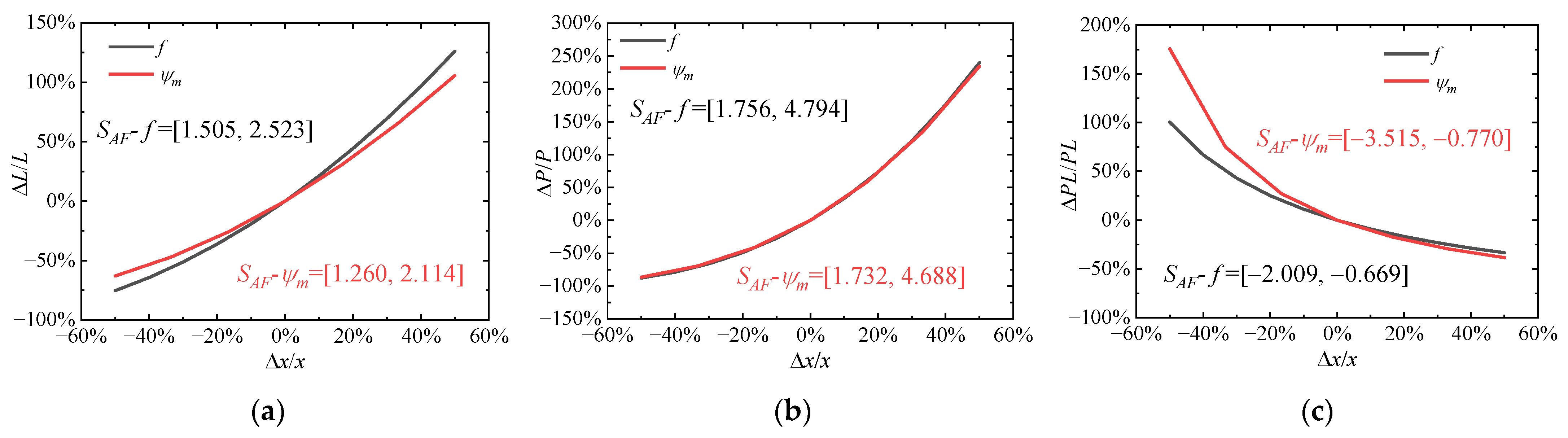
| f | 2.014 | 0.999 | 3.017 | 0.999 | −1.003 | 0.999 |
| ψm | 1.415 | 0.983 | 2.876 | 0.999 | −1.462 | 0.992 |
Disclaimer/Publisher’s Note: The statements, opinions and data contained in all publications are solely those of the individual author(s) and contributor(s) and not of MDPI and/or the editor(s). MDPI and/or the editor(s) disclaim responsibility for any injury to people or property resulting from any ideas, methods, instructions or products referred to in the content. |
© 2023 by the authors. Licensee MDPI, Basel, Switzerland. This article is an open access article distributed under the terms and conditions of the Creative Commons Attribution (CC BY) license (https://creativecommons.org/licenses/by/4.0/).
Share and Cite
Lang, X.; Song, B.; Yang, W.; Yang, X.; Xue, D. Sensitivity Analysis of Wing Geometric and Kinematic Parameters for the Aerodynamic Performance of Hovering Flapping Wing. Aerospace 2023, 10, 74. https://doi.org/10.3390/aerospace10010074
Lang X, Song B, Yang W, Yang X, Xue D. Sensitivity Analysis of Wing Geometric and Kinematic Parameters for the Aerodynamic Performance of Hovering Flapping Wing. Aerospace. 2023; 10(1):74. https://doi.org/10.3390/aerospace10010074
Chicago/Turabian StyleLang, Xinyu, Bifeng Song, Wenqing Yang, Xiaojun Yang, and Dong Xue. 2023. "Sensitivity Analysis of Wing Geometric and Kinematic Parameters for the Aerodynamic Performance of Hovering Flapping Wing" Aerospace 10, no. 1: 74. https://doi.org/10.3390/aerospace10010074