
Comparison of Flood Frequency at Different Climatic Scenarios in Forested Coastal Watersheds


Abstract
:1. Introduction
2. Materials and Methods
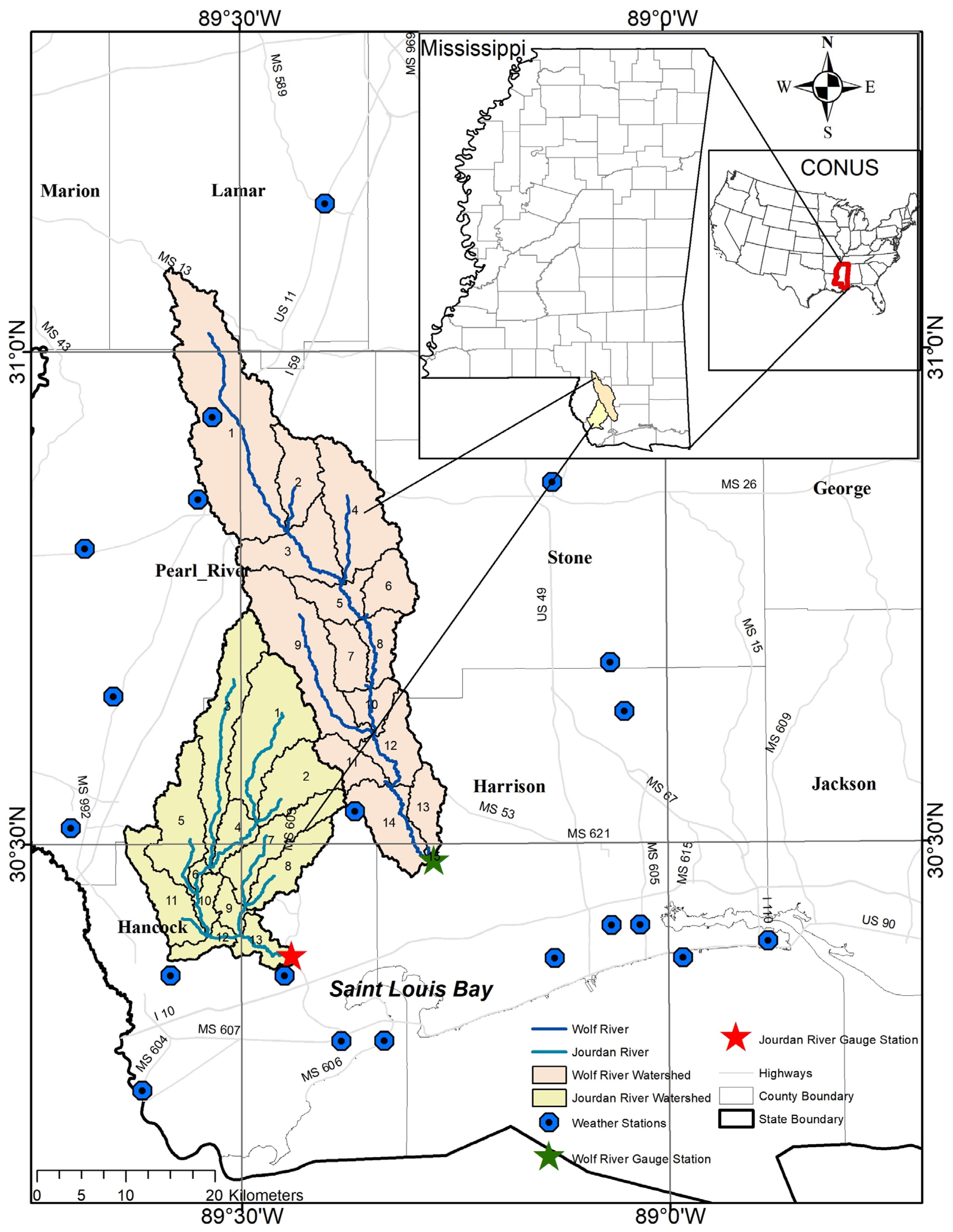
2.1. Study Area
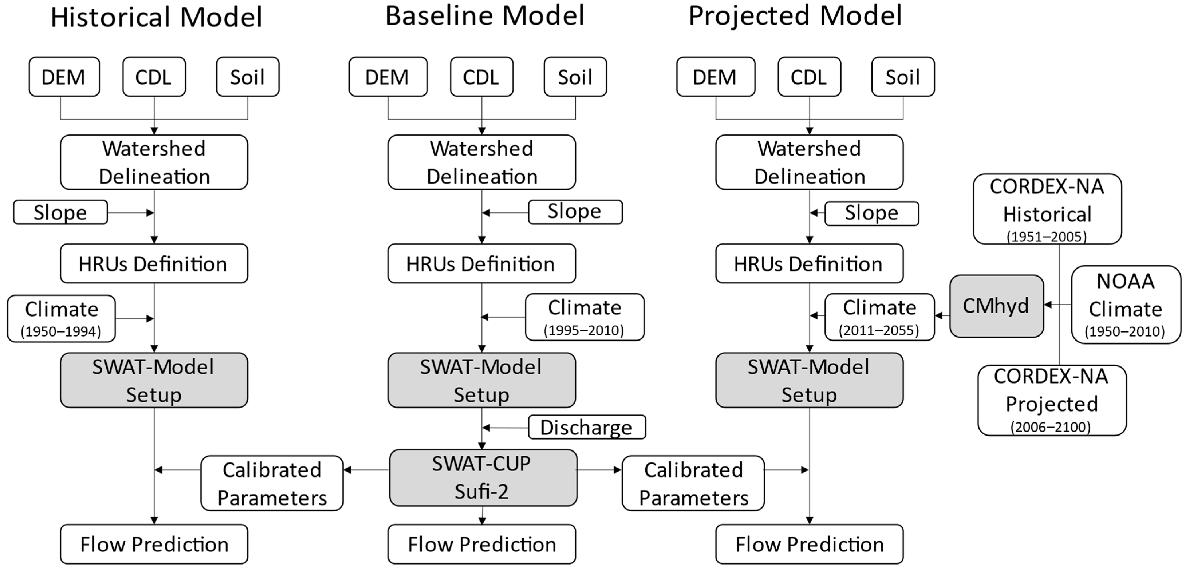
2.2. Model Setup
2.3. Model Evaluation
2.4. Flood Frequency Analysis
3. Results
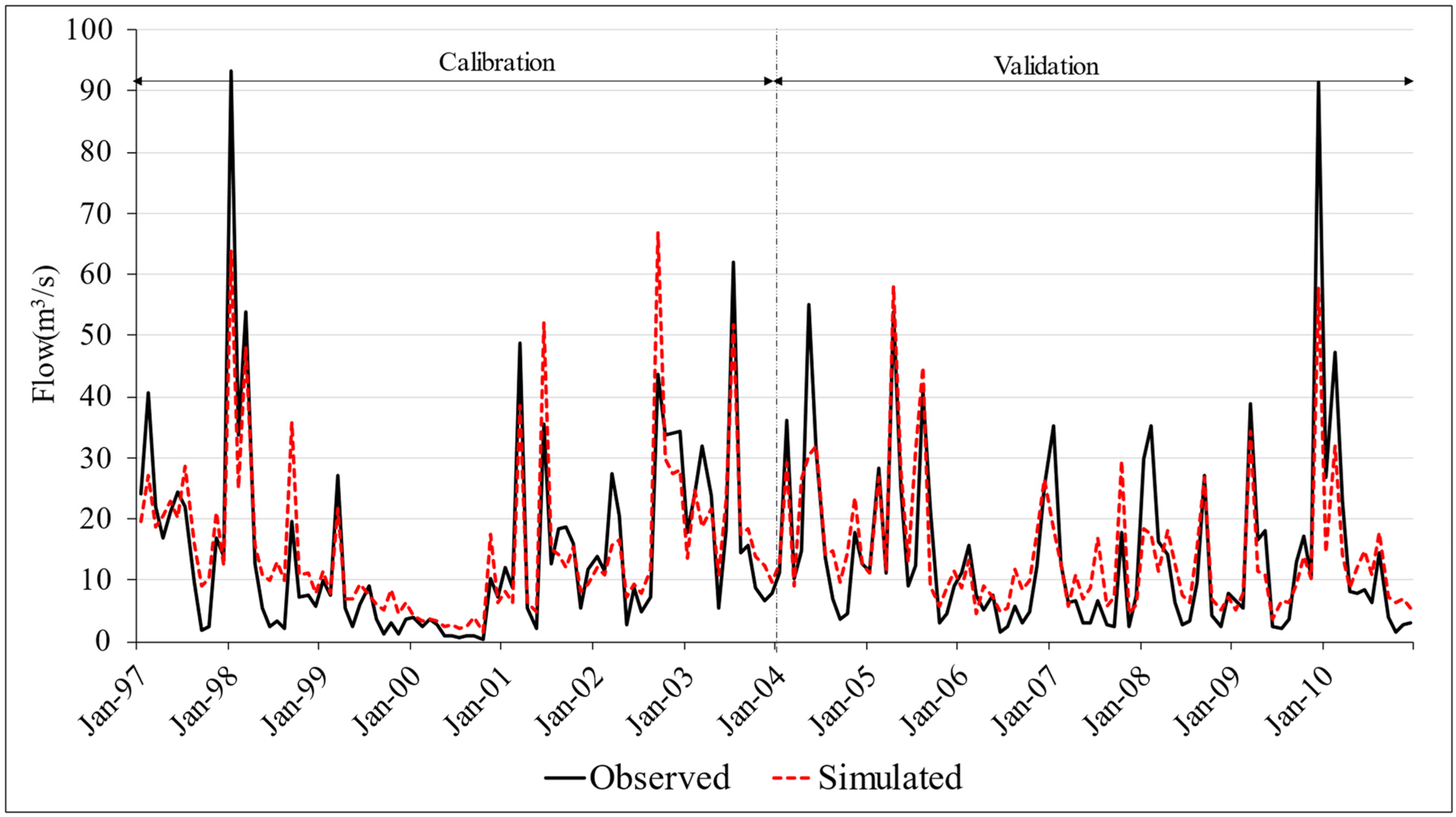
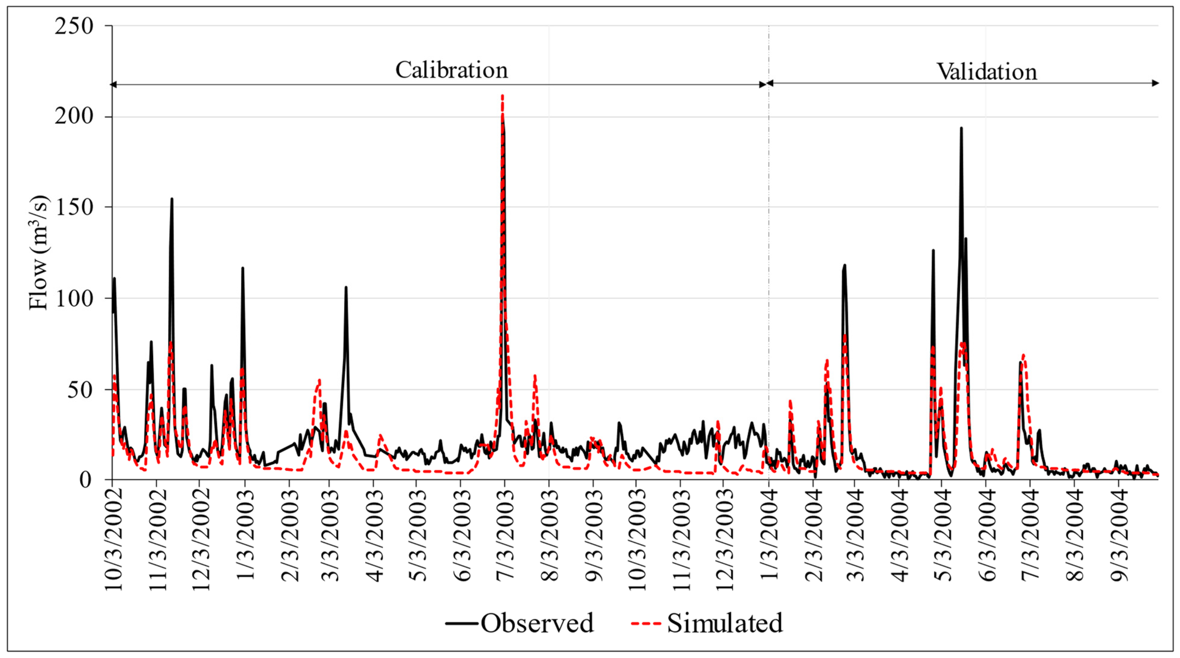
3.1. Streamflow Calibration and Validation
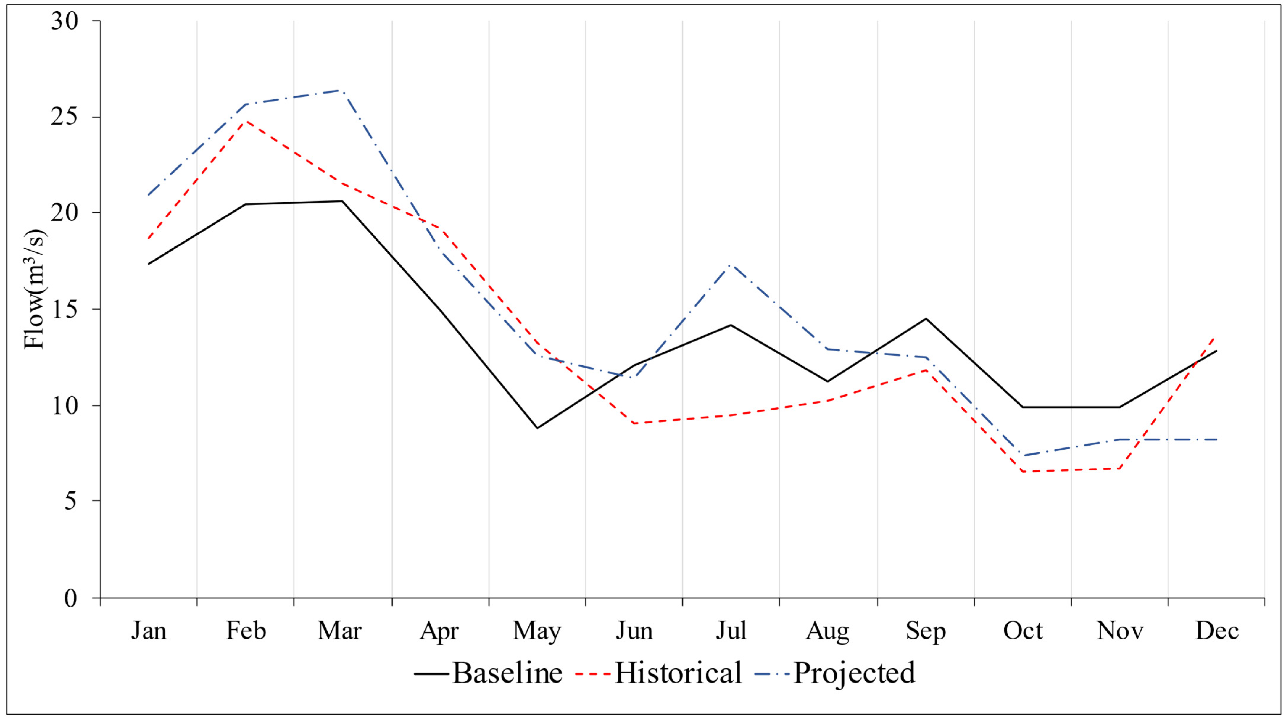
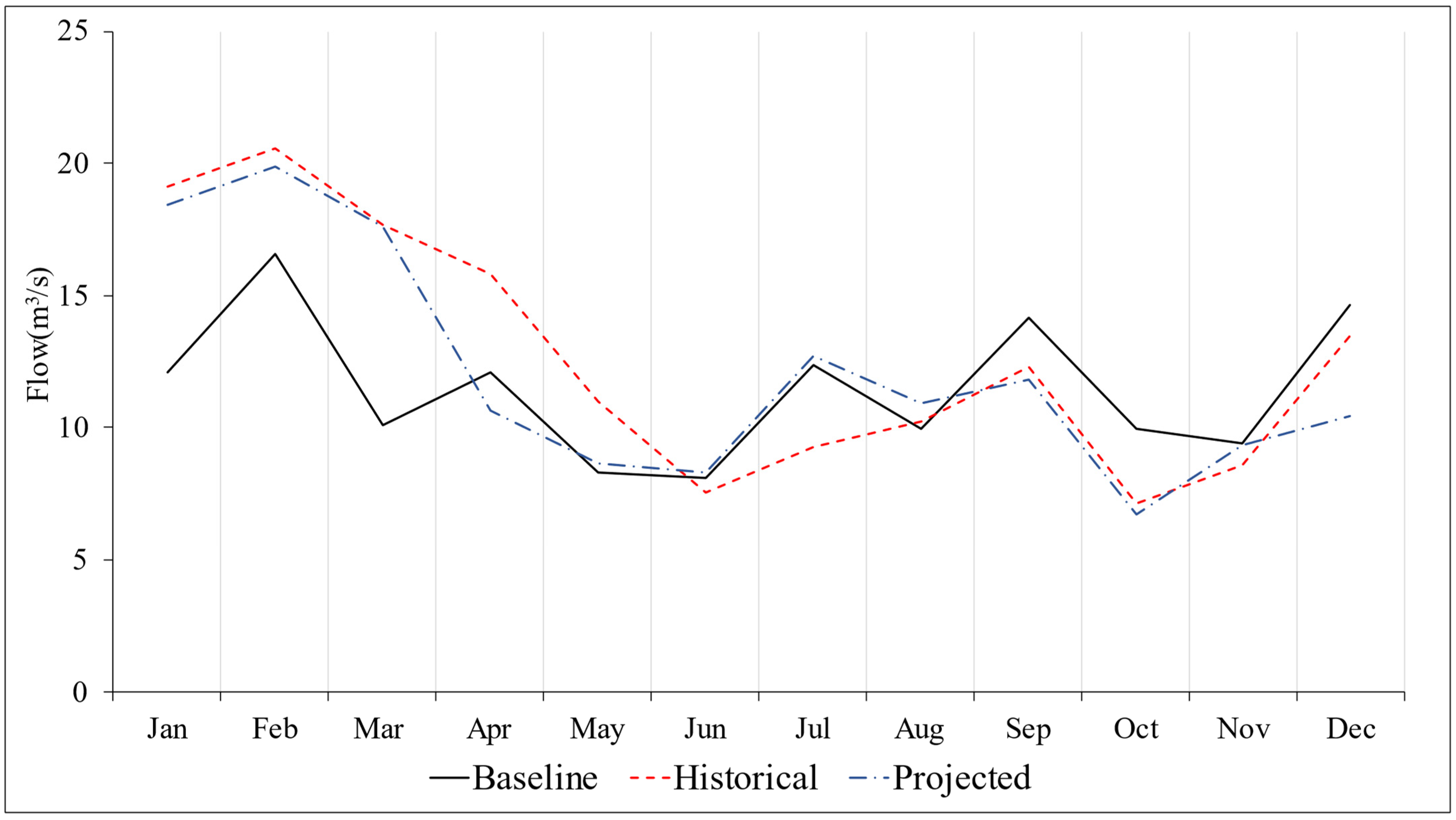
3.2. Flow Comparison of Different Climate Conditions
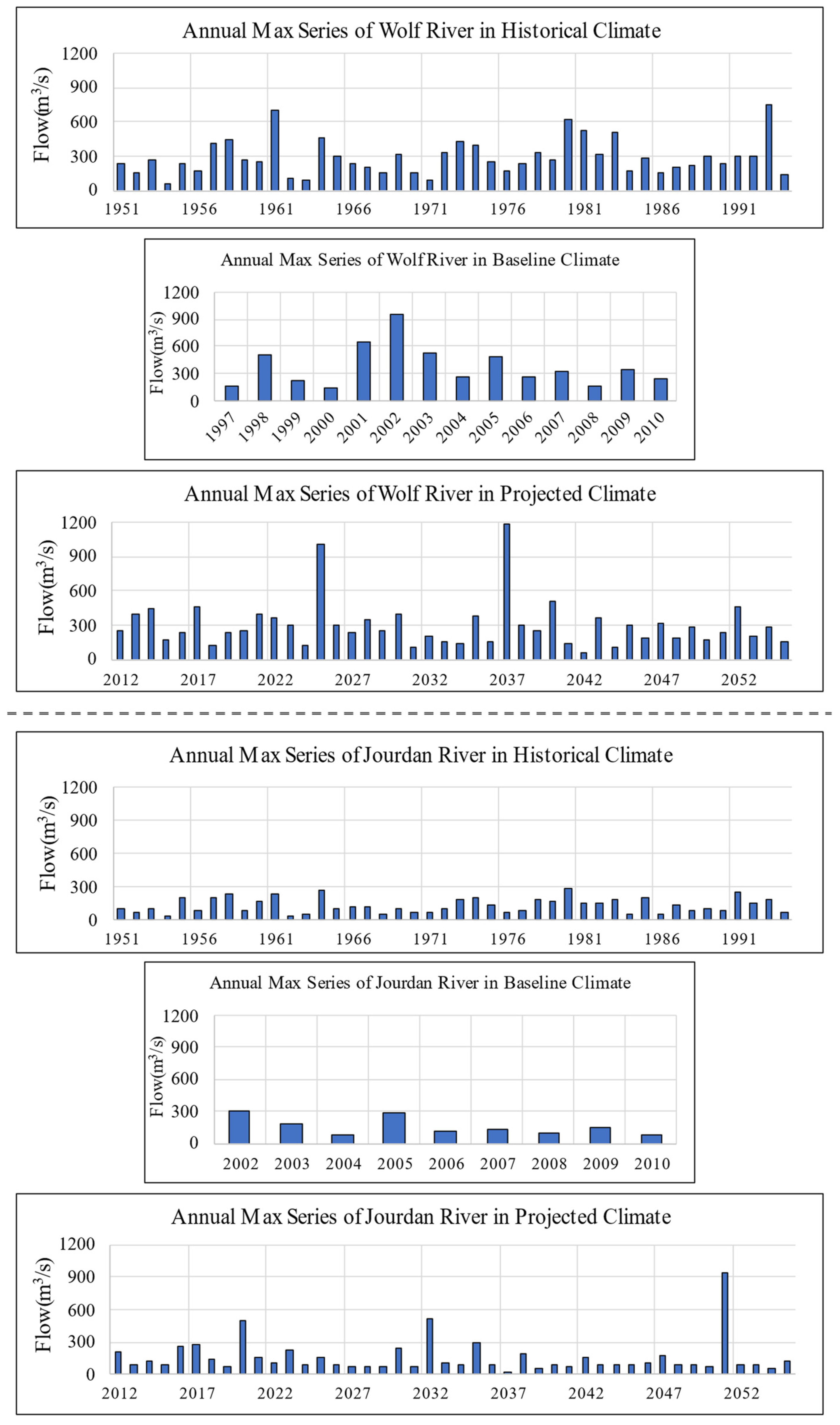
3.3. Flow Extreme Events
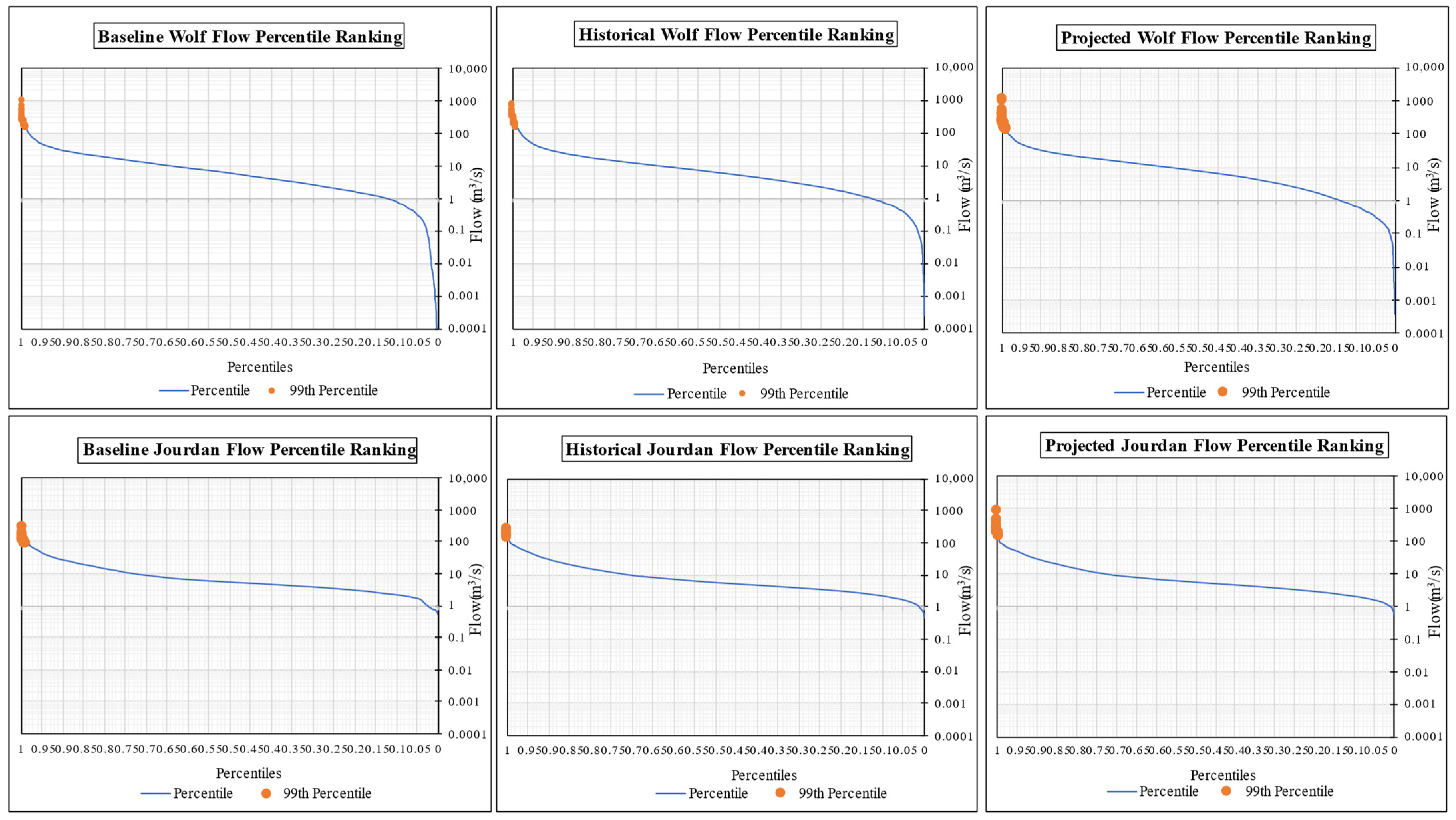
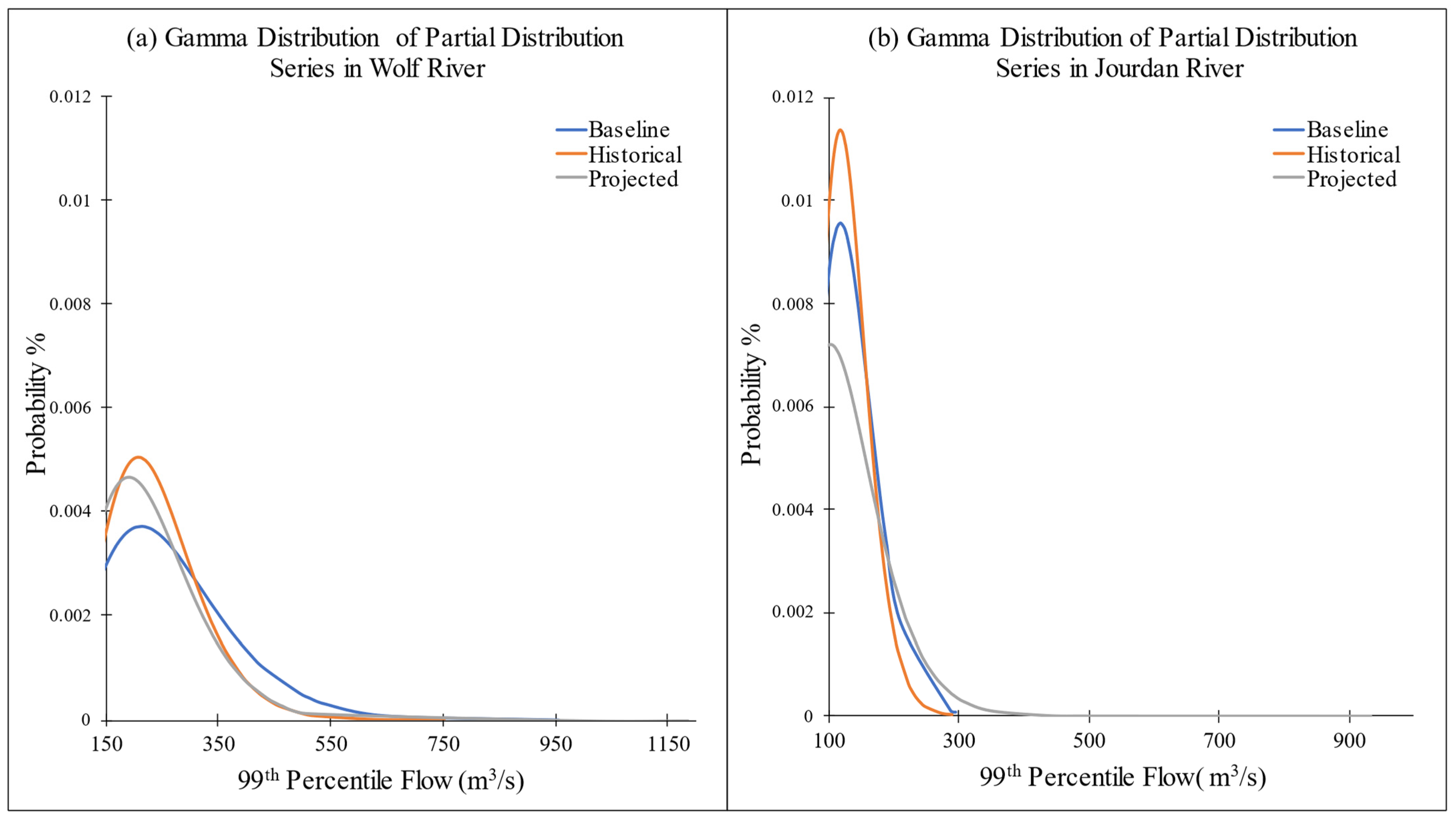
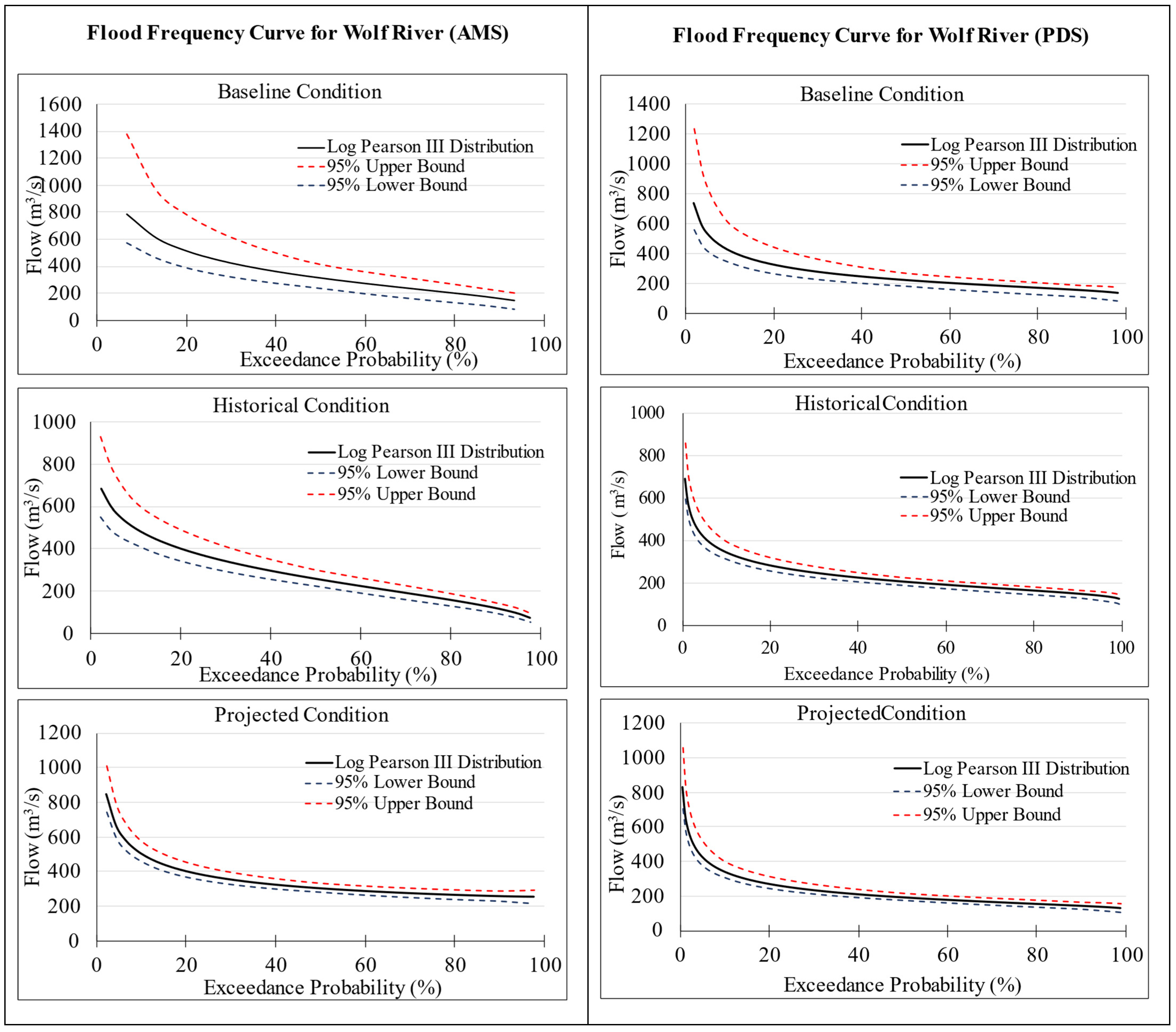
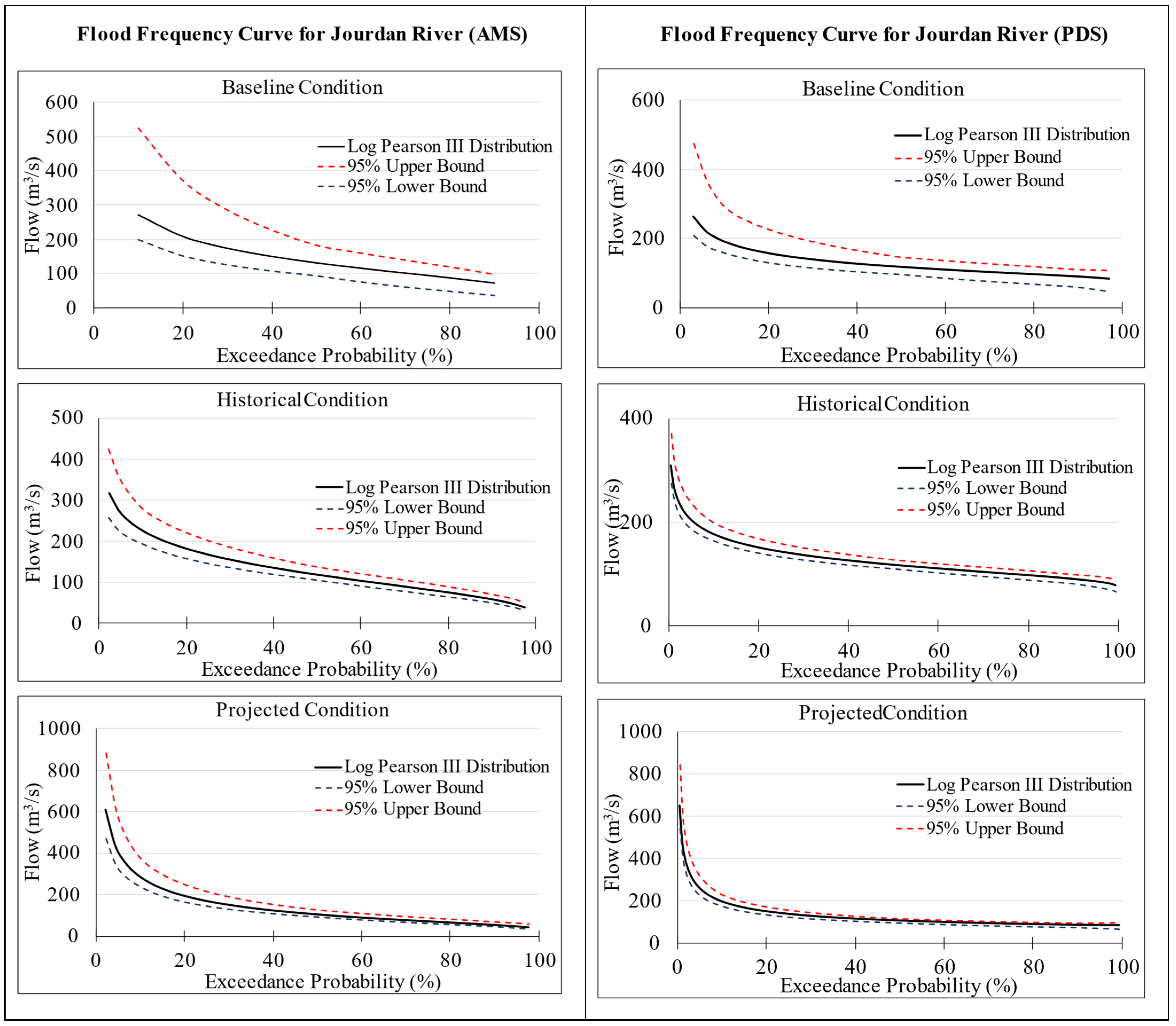
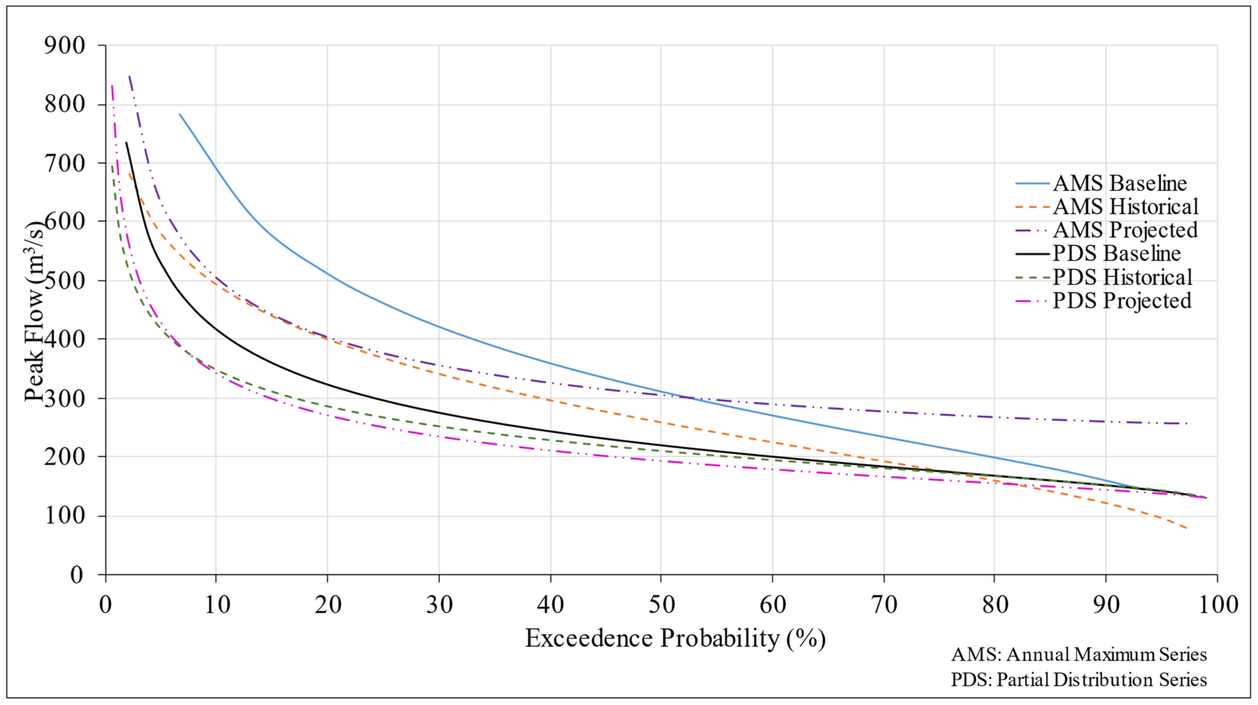
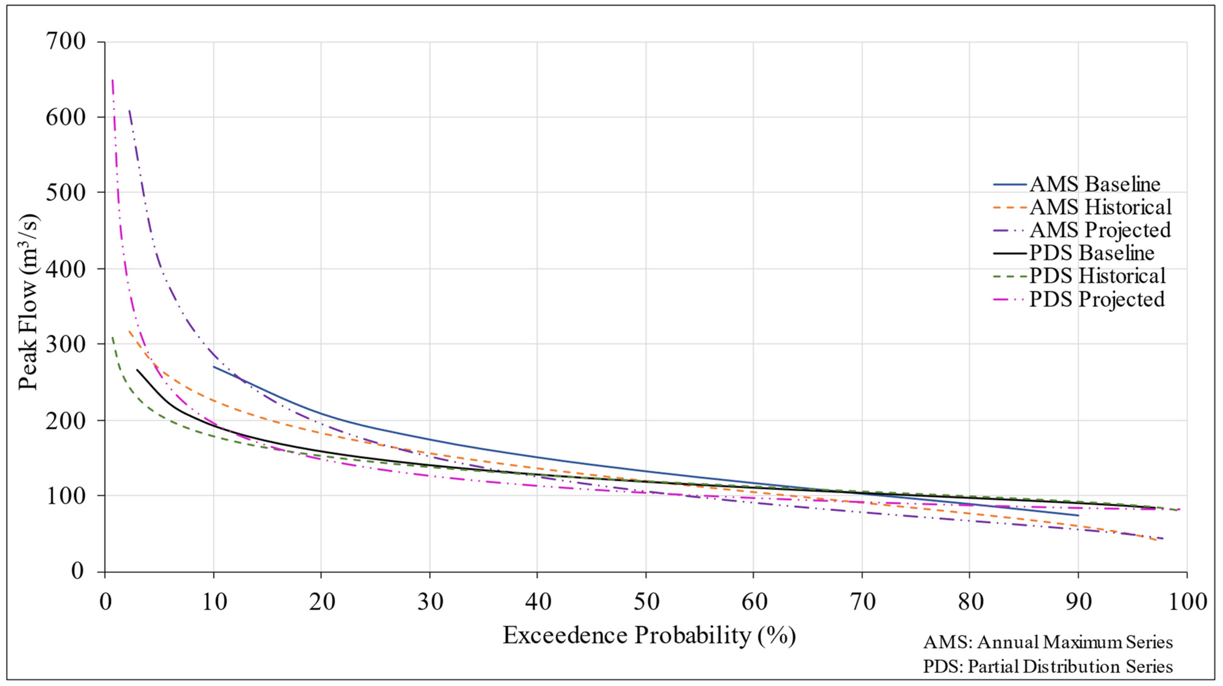
3.4. Flood Frequency Analysis
4. Discussion
5. Conclusions
Author Contributions
Funding
Institutional Review Board Statement
Informed Consent Statement
Data Availability Statement
Acknowledgments
Conflicts of Interest
References
- Pörtner, H.O. (Ed.) Climate Change 2022: Impacts, Adaptation and Vulnerability Working Group II Contribution to the Sixth Assessment Report of the Intergovernmental Panel on Climate Change; Cambridge University Press: Cambridge, UK, 2022. [Google Scholar] [CrossRef]
- Lee, C.H.; Yeh, H.F. Impact of Climate Change and Human Activities on Streamflow Variations Based on the Budyko Framework. Water 2019, 11, 2001. [Google Scholar] [CrossRef]
- Chiang, L.C.; Liao, C.J.; Lu, C.M.; Wang, Y.C. Applicability of Modified SWAT Model (SWAT-Twn) on Simulation of Watershed Sediment Yields under Different Land Use/Cover Scenarios in Taiwan. Environ. Monit. Assess. 2021, 193, 1–23. [Google Scholar] [CrossRef] [PubMed]
- Giorgi, F.; Raffaele, F.; Coppola, E. The Response of Precipitation Characteristics to Global Warming from Climate Projections. Earth Syst. Dyn. 2019, 10, 73–89. [Google Scholar] [CrossRef]
- Pachauri, R.K.; Allen, M.R.; Barros, V.R.; Broome, J.; Cramer, W.; Christ, R.; Church, J.A.; Clarke, L.; Dahe, Q.; Dasgupta, P.; et al. Climate Change 2014: Synthesis Report; Contribution of Working Groups I, II and III to the Fifth Assessment Report of the Intergovernmental Panel on Climate Change; IPCC: Geneva, Switzerland, 2014; p. 151. [Google Scholar]
- Merkens, J.L.; Reimann, L.; Hinkel, J.; Vafeidis, A.T. Gridded Population Projections for the Coastal Zone under the Shared Socioeconomic Pathways. Glob. Planet. Change 2016, 145, 57–66. [Google Scholar] [CrossRef]
- Kron, W. Coasts: The High-Risk Areas of the World. Nat. Hazards 2013, 66, 1363–1382. [Google Scholar] [CrossRef]
- Boithias, L.; Sauvage, S.; Lenica, A.; Roux, H.; Abbaspour, K.C.; Larnier, K.; Dartus, D.; Sánchez-Pérez, J.M. Simulating Flash Floods at Hourly Time-Step Using the SWAT Model. Water 2017, 9, 929. [Google Scholar] [CrossRef]
- Zhang, K.; Shalehy, M.H.; Ezaz, G.T.; Chakraborty, A.; Mohib, K.M.; Liu, L. An Integrated Flood Risk Assessment Approach Based on Coupled Hydrological-Hydraulic Modeling and Bottom-up Hazard Vulnerability Analysis. Environ. Model. Softw. 2022, 148, 105279. [Google Scholar] [CrossRef]
- Chao, L.; Zhang, K.; Li, Z.; Wang, J.; Yao, C.; Li, Q. Applicability Assessment of the CASCade Two Dimensional SEDiment (CASC2D-SED) Distributed Hydrological Model for Flood Forecasting across Four Typical Medium and Small Watersheds in China. J. Flood Risk Manag. 2019, 12, e12518. [Google Scholar] [CrossRef]
- Jodar-Abellan, A.; Valdes-Abellan, J.; Pla, C.; Gomariz-Castillo, F. Impact of Land Use Changes on Flash Flood Prediction Using a Sub-Daily SWAT Model in Five Mediterranean Ungauged Watersheds (SE Spain). Sci. Total Environ. 2019, 657, 1578–1591. [Google Scholar] [CrossRef]
- Li, W.; Lin, K.; Zhao, T.; Lan, T.; Chen, X.; Du, H.; Chen, H. Risk Assessment and Sensitivity Analysis of Flash Floods in Ungauged Basins Using Coupled Hydrologic and Hydrodynamic Models. J. Hydrol. 2019, 572, 108–120. [Google Scholar] [CrossRef]
- Nkwunonwo, U.C.; Whitworth, M.; Baily, B. A Review of the Current Status of Flood Modelling for Urban Flood Risk Management in the Developing Countries. Sci. Afr. 2020, 7, e00269. [Google Scholar] [CrossRef]
- Arnold, J.G.; Srinivasan, R.; Muttiah, R.S.; Williams, J.R. Large Area Hydrologic Modeling and Assessment Part I: Model Development 1. J. Am. Water Resour. Assoc. 1998, 34, 73–89. [Google Scholar] [CrossRef]
- Roux, H.; Labat, D.; Garambois, P.A.; Maubourguet, M.M.; Chorda, J.; Dartus, D. A Physically-Based Parsimonious Hydrological Model for Flash Floods in Mediterranean Catchments. Nat. Hazards Earth Syst. Sci. 2011, 11, 2567–2582. [Google Scholar] [CrossRef]
- Brunner, G.W. HEC-RAS River Analysis System. Hydraulic Reference Manual. Version 1.0. Hydrologic Engineering Center Davis CA. 1995. Available online: https://www.hec.usace.army.mil/confluence/rasdocs/ras1dtechref/latest (accessed on 2 December 2022).
- Kastridis, A.; Stathis, D. Evaluation of Hydrological and Hydraulic Models Applied in Typical Mediterranean Ungauged Watersheds Using Post-Flash-Flood Measurements. Hydrology 2020, 7, 12. [Google Scholar] [CrossRef]
- Feldman, A.D. Hydrologic Modeling System HEC-HMS Technical Reference Manual; US Army Corps of Engineers, Hydrologic Engineering Center: Davis, CA, USA, 2000. [Google Scholar]
- Julien, P.Y.; Saghafian, B. CASC2D User’s Manual: A Two-Dimensional Watershed Rainfall-Runoff Model; Diss. Colorado State University. Libraries 1991, 1–66. [Google Scholar]
- Beven, K.J.; Kirkby, M.J. A Physically Based, Variable Contributing Area Model of Basin Hydrology. Hydrol. Sci. J. 1979, 24, 43–69. [Google Scholar] [CrossRef]
- MIKE FLOOD 1D-2D and 1D-3D Modelling User Manual. DHI Water Environ. 2021, 1–154.
- Ajmal, A.; Irfan, S.; Sabahat, N.; Saleem, S.B. Analysis of Flood Risk Management in the Context of Mathematical Models. In Proceedings of the 2019 International Conference on Innovative Computing (ICIC)2019, Lahore, Pakistan, 1–2 November 2019; pp. 1–6. [Google Scholar] [CrossRef]
- Iqbal, M.S.; Dahri, Z.H.; Querner, E.P.; Khan, A.; Hofstra, N. Impact of Climate Change on Flood Frequency and Intensity in the Kabul River Basin. Geosciences 2018, 8, 114. [Google Scholar] [CrossRef]
- Khan, S.I.; Hong, Y.; Wang, J.; Yilmaz, K.K.; Gourley, J.J.; Adler, R.F.; Brakenridge, G.R.; Policelli, F.; Habib, S.; Irwin, D. Satellite Remote Sensing and Hydrologic Modeling for Flood Inundation Mapping in Lake Victoria Basin: Implications for Hydrologic Prediction in Ungauged Basins. IEEE Trans. Geosci. Remote Sens. 2010, 49, 85–95. [Google Scholar] [CrossRef]
- SWAT Literature Database for Peer-Reviewed Journal Articles. Center for Agricultural and Rural Development, Ames, IA, USA. 2022. Available online: https://www.card.iastate.edu/swat_articles/ (accessed on 1 December 2022).
- Parajuli, P.B.; Risal, A. Evaluation of Climate Change on Streamflow, Sediment, and Nutrient Load at Watershed Scale. Climate 2021, 9, 165. [Google Scholar] [CrossRef]
- Bhatta, B.; Shrestha, S.; Shrestha, P.K.; Talchabhadel, R. Evaluation and Application of a SWAT Model to Assess the Climate Change Impact on the Hydrology of the Himalayan River Basin. Catena 2019, 181, 104082. [Google Scholar] [CrossRef]
- Kiesel, J.; Gericke, A.; Rathjens, H.; Wetzig, A.; Kakouei, K.; Jähnig, S.C.; Fohrer, N. Climate Change Impacts on Ecologically Relevant Hydrological Indicators in Three Catchments in Three European Ecoregions. Ecol. Eng. 2019, 127, 404–416. [Google Scholar] [CrossRef]
- Nguyen, H.H.; Recknagel, F.; Meyer, W.; Frizenschaf, J.; Shrestha, M.K. Modelling the Impacts of Altered Management Practices, Land Use and Climate Changes on the Water Quality of the Millbrook Catchment-Reservoir System in South Australia. J. Environ. Manag. 2017, 202, 1–11. [Google Scholar] [CrossRef] [PubMed]
- Rabezanahary Tanteliniaina, M.F.; Rahaman, M.H.; Zhai, J. Assessment of the Future Impact of Climate Change on the Hydrology of the Mangoky River, Madagascar Using ANN and SWAT. Water 2021, 13, 1239. [Google Scholar] [CrossRef]
- Singh, V.; Sharma, A.; Goyal, M.K. Projection of Hydro-Climatological Changes over Eastern Himalayan Catchment by the Evaluation of RegCM4 RCM and CMIP5 GCM Models. Hydrol. Res. 2019, 50, 117–137. [Google Scholar] [CrossRef]
- Menna, B.Y. Simulation of Hydro Climatological Impacts Caused by Climate Change: The Case of Hare Watershed, Southern Rift Valley of Ethiopia. Hydrol Curr. Res. 2017, 8, 2. [Google Scholar] [CrossRef]
- Devkota, L.P.; Gyawali, D.R. Impacts of Climate Change on Hydrological Regime and Water Resources Management of the Koshi River Basin, Nepal. J. Hydrol. Reg. Stud. 2015, 4, 502–515. [Google Scholar] [CrossRef]
- Maghsood, F.F.; Moradi, H.; Massah Bavani, A.R.; Panahi, M.; Berndtsson, R.; Hashemi, H. Climate Change Impact on Flood Frequency and Source Area in Northern Iran under CMIP5 Scenarios. Water 2019, 11, 273. [Google Scholar] [CrossRef]
- Upadhyay, P.; Linhoss, A.; Kelble, C.; Ashby, S.; Murphy, N.; Parajuli, P.B. Applications of the SWAT Model for Coastal Watersheds: Review and Recommendations. J. ASABE 2022, 65, 453–469. [Google Scholar] [CrossRef]
- Kundzewicz, Z.W. Climate Change Impacts on the Hydrological Cycle. Ecohydrol. Hydrobiol. 2008, 8, 195–203. [Google Scholar] [CrossRef] [Green Version]
- Wuebbles, D.; Fahey, D.; Takle, E.; Hibbard, K.; Arnold, J.; DeAngelo, B.; Doherty, S.; Easterling, D.; Edmonds, J.; Edmonds, T.; et al. Climate Science Special Report: Fourth National Climate Assessment (NCA4), Volume I; U.S. Global Change Research Program: Washington, DC, USA, 2017.
- Kunkel, K.E.; Frankson, R.; Runkle, J.; Champion, S.M.; Stevens, L.E.; Easterling, D.R.; Stewart, B.C.; McCarrick, A.; Lemery, C.R. State Climate Summaries for the United States 2022. NOAA Technical Report NESDIS 150. NOAA NESDIS. 2022. Available online: https://www.nesdis.noaa.gov/about/documents-reports/technical-reports (accessed on 4 October 2022).
- Sankar, M.S.; Dash, P.; Lu, Y.; Hu, X.; Mercer, A.E.; Wickramarathna, S.; Beshah, W.T.; Sanders, L.; Arslan, Z.; Dyer, J.; et al. Seasonal Changes of Trace Metal-Nutrient-Dissolved Organic Matter Conveyance along with Coastal Acidification over the Largest Oyster Reef in Western Mississippi Sound, Northern Gulf of Mexico. North. Gulf Mex. 2021. [Google Scholar] [CrossRef]
- Parra, S.M.; Sanial, V.; Boyette, A.D.; Cambazoglu, M.K.; Soto, I.M.; Greer, A.T.; Chiaverano, L.M.; Hoover, A.; Dinniman, M.S. Bonnet Carré Spillway Freshwater Transport and Corresponding Biochemical Properties in the Mississippi Bight. Cont. Shelf Res. 2020, 199, 104114. [Google Scholar] [CrossRef]
- Dile, Y.T.; Daggupati, P.; George, C.; Srinivasan, R.; Arnold, J. Introducing a New Open Source GIS User Interface for the SWAT Model. Environ. Model. Softw. 2016, 85, 129–138. [Google Scholar] [CrossRef]
- Neitsch, S.L.; Arnold, J.G.; Kiniry, J.R.; Srinivasan, R.; Williams, J.R. Soil and Water Assessment Tool User’s Manual, Version 2000; Texas Water Resources Institute: College Station, TX, USA, 2000; pp. 1–27. [Google Scholar]
- USGS The National Map-Advanced Viewer. Available online: https://apps.nationalmap.gov/viewer/ (accessed on 4 October 2022).
- Global Data | SWAT | Soil & Water Assessment Tool. Available online: https://swat.tamu.edu/data/ (accessed on 4 October 2022).
- CropScape-NASS CDL Program. Available online: https://nassgeodata.gmu.edu/CropScape/ (accessed on 4 October 2022).
- Abbaspour, K.C. Swat-Cup 2012. SWAT Calibration and Uncertainty Program—A User Manual; Swiss Federal Institute of Aquatic Science and Technology: Dübendorf, Switzerland, 2013. [Google Scholar]
- Sao, D.; Kato, T.; Tu, L.H.; Thouk, P.; Fitriyah, A.; Oeurng, C. Evaluation of Different Objective Functions Used in the SUFI-2 Calibration Process of SWAT-CUP on Water Balance Analysis: A Case Study of the Pursat River Basin, Cambodia. Water 2020, 12, 2901. [Google Scholar] [CrossRef]
- Gupta, H.V.; Kling, H.; Yilmaz, K.K.; Martinez, G.F. Decomposition of the Mean Squared Error and NSE Performance Criteria: Implications for Improving Hydrological Modelling. J. Hydrol. 2009, 377, 80–91. [Google Scholar] [CrossRef]
- Mearns, L.; McGinnis, S.; Korytina, D.; Arritt, R.; Biner, S.; Bukovsky, M.; Chang, H.; Christensen, O.; Herzmann, D.; Jiao, Y.; et al. 2017: The NA-CORDEX Dataset, Version 1.0. NCAR Climate Data Gateway, Boulder CO. 2017. Available online: https://na-cordex.org/ (accessed on 14 October 2022). [CrossRef]
- Software | SWAT | Soil & Water Assessment Tool. Available online: https://swat.tamu.edu/software/ (accessed on 20 January 2021).
- Rathjens, H.; Bieger, K.; Srinivasan, R.; Chaubey, I.; Arnold, J.G. CMhyd User Manual Documentation for Preparing Simulated Climate Change Data for Hydrologic Impact Studies. 2016. Available online: http://swat.tamu.edu/software/cmhyd (accessed on 15 October 2022).
- Krause, P.; Boyle, D.P.; Bäse, F. Comparison of Different Efficiency Criteria for Hydrological Model Assessment. Adv. Geosci. 2005, 5, 89–97. [Google Scholar] [CrossRef]
- Nash, J.E.; Sutcliffe, J.V. River Flow Forecasting through Conceptual Models Part I-A Discussion of Principles. J. Hydrol. 1970, 10, 282–290. [Google Scholar] [CrossRef]
- Gupta, H.V.; Sorooshian, S.; Yapo, P.O. Status of Automatic Calibration for Hydrologic Models: Comparison with Multilevel Expert Calibration. J. Hydrol. Eng. 1999, 4, 135–143. [Google Scholar] [CrossRef]
- Moriasi, D.N.; Gitau, M.W.; Pai, N.; Daggupati, P.; Gitau, M.W.; Member, A.; Moriasi, D.N. Hydrologic and Water Quality Models: Performance Measures and Evaluation Criteria. Trans. ASABE 2015, 58, 1763–1785. [Google Scholar] [CrossRef] [Green Version]
- Brighenti, T.M.; Bonumá, N.B.; Grison, F.; de Almeida Mota, A.; Kobiyama, M.; Chaffe, P.L.B. Two Calibration Methods for Modeling Streamflow and Suspended Sediment with the SWAT Model. Ecol. Eng. 2019, 127, 103–113. [Google Scholar] [CrossRef]
- Chow, V.T.; Maidment, D.R.; Mays, L.W. Applied Hydrology McGraw-Hill International Editions; McGraw-Hill Science/Engineering/Math: New York, NY, USA, 1988. [Google Scholar]
- Subcommittee, H. USGS Interagency Advisory Committee on Water Data; Office of Water Data Coordination, US Geologic Survey: Reston, VA, USA, 1986. Available online: https://water.usgs.gov/osw/bulletin17b/dl_flow.pdf (accessed on 9 November 2022).
- Mayo, T.L.; Lin, N. Climate Change Impacts to the Coastal Flood Hazard in the Northeastern United States. Weather Clim. Extrem. 2022, 36, 100453. [Google Scholar] [CrossRef]


| S. No. | Data | Source |
|---|---|---|
| 1 | Elevation Data: Digital Elevation Model (DEM) (30 m × 30 m) (2020) | United States Geological Survey (USGS) (http://viewer.nationalmap.gov/viewer/) (accessed on 4 October 2022) |
| 2 | Land-use and Land-cover Data: Cropland Data Layer (CDL) (2010) | United States Department of Agriculture-National Agricultural Statistics Service (USDA-NASS) (http://nassgeodata.gmu.edu/CropScape/) (accessed on 4 October 2022) |
| 3 | Soil Data: USSURGO (2020) | United States Soil Survey Geographic Database (US-SSURGO) SWAT-USSURGO (https://swat.tamu.edu/data/) (accessed on 4 October 2022) |
| 4 | Weather Data: NOAA (1995–2010) Precipitation, Maximum Temperature, Minimum Temperature | National Oceanic and Atmospheric Administration (NOAA) SWAT—Climate Data (https://swat.tamu.edu/data/) (accessed on 4 October 2022) |
| 5 | Discharge Data: -USGS 02481510 (1997–2010) (Wolf River Nr Landon) -USGS 02481660 (2002–2005) (Jourdan River Nr Bay St Louis) | United States Geological Survey (USGS) (https://waterdata.usgs.gov/ms/nwis/) (accessed on 5 October 2022) |
| Parameters | Description | Fitted Value |
|---|---|---|
| CN2 | Initial SCS runoff curve number for moisture condition II. | 0.133 |
| ALPHA_BF | Baseflow alpha factor (days). | 0.316 |
| ESCO | Soil evaporation compensation factor. | 0.217 |
| SOL_K | Saturated hydraulic conductivity. | −0.018 |
| SOL_BD | Moist bulk density. | 0.104 |
| SOL_AWC | Available water capacity of the soil layer. | 0.297 |
| Parameters | Description | Fitted Value |
|---|---|---|
| ALPHA_BF | Baseflow alpha factor (days). | 0.917 |
| ESCO | Soil evaporation compensation factor. | 0.910 |
| GW_DELAY | Groundwater delay (days). | 1.126 |
| GWQMN | Threshold depth of water in the shallow aquifer required for return flow to occur (mm). | 874.982 |
| EPCO | Plant uptake compensation factor. | 0.698 |
| CN2 | Initial SCS runoff curve number for moisture condition II. | −0.194 |
| RCHRG_DP | Deep aquifer percolation fraction. | 0.391 |
| REVAPMN | Threshold depth of water in the shallow aquifer for “revap” to occur (mm). | 177.726 |
| SOL_K | Saturated hydraulic conductivity. | −0.139 |
| SOL_BD | Moist bulk density. | 0.223 |
| SOL_AWC | Available water capacity of the soil layer. | 0.038 |
| OV_N | Manning’s “n” value for overland flow. | −0.010 |
| CANMX | Maximum canopy storage. | 93.562 |
| SLSUBBSN | Average slope length. | 0.386 |
| LAT_TTIME | Lateral flow travel time. | 3.238 |
| CNCOEF | Plant ET curve number coefficient. | 0.678 |
| CH_N2 | Manning’s “n” value for the main channel. | 0.023 |
| CH_K2 | Effective hydraulic conductivity in main channel alluvium. | 65.951 |
| HRU_SLP | Average slope steepness. | 0.361 |
| Watershed | Model Development | R2 | NSE | PBIAS | KGE |
|---|---|---|---|---|---|
| WRW | Calibration (January 1997–December 2003) | 0.82 | 0.81 | −4.9 | 0.80 |
| Validation (January 2004–December 2010) | 0.75 | 0.73 | −3.0 | 0.70 | |
| JRW | Calibration (10 March 2002–31 December 2003) | 0.59 | 0.42 | 36.7 | 0.55 |
| Validation (1 January 2004–30 September 2004) | 0.72 | 0.71 | 4.7 | 0.68 |
Disclaimer/Publisher’s Note: The statements, opinions and data contained in all publications are solely those of the individual author(s) and contributor(s) and not of MDPI and/or the editor(s). MDPI and/or the editor(s) disclaim responsibility for any injury to people or property resulting from any ideas, methods, instructions or products referred to in the content. |
© 2023 by the authors. Licensee MDPI, Basel, Switzerland. This article is an open access article distributed under the terms and conditions of the Creative Commons Attribution (CC BY) license (https://creativecommons.org/licenses/by/4.0/).
Share and Cite
Bhattarai, S.; Parajuli, P.B.; To, F. Comparison of Flood Frequency at Different Climatic Scenarios in Forested Coastal Watersheds. Climate 2023, 11, 41. https://doi.org/10.3390/cli11020041
Bhattarai S, Parajuli PB, To F. Comparison of Flood Frequency at Different Climatic Scenarios in Forested Coastal Watersheds. Climate. 2023; 11(2):41. https://doi.org/10.3390/cli11020041
Chicago/Turabian StyleBhattarai, Shreeya, Prem B. Parajuli, and Filip To. 2023. "Comparison of Flood Frequency at Different Climatic Scenarios in Forested Coastal Watersheds" Climate 11, no. 2: 41. https://doi.org/10.3390/cli11020041