Article

Climate Change Impacts on Streamflow in the Krishna River Basin, India: Uncertainty and Multi-Site Analysis

by
Ponguru Naga Sowjanya
1,
Venkata Reddy Keesara
2,
Shashi Mesapam
2,
Jew Das
2 and
Venkataramana Sridhar
3,*
1
Department of Civil Engineering, Narasaraopeta Engineering College, Narasaraopeta 522601, India
2
Department of Civil Engineering, National Institute of Technology Warangal, Warangal 506004, India
3
Department of Biological Systems Engineering, Virginia Polytechnic Institute and State University, Blacksburg, VA 24061, USA
*
Author to whom correspondence should be addressed.
Climate 2022, 10(12), 190; https://doi.org/10.3390/cli10120190
Submission received: 18 October 2022 / Revised: 24 November 2022 / Accepted: 26 November 2022 / Published: 1 December 2022

Abstract

:
In Peninsular India, the Krishna River basin is the second largest river basin that is overutilized and more vulnerable to climate change. The main aim of this study is to determine the future projection of monthly streamflows in the Krishna River basin for Historic (1980–2004) and Future (2020–2044, 2045–2069, 2070–2094) climate scenarios (RCP 4.5 and 8.5, respectively), with the help of the Soil Water and Assessment Tool (SWAT). SWAT model parameters are optimized using SWAT-CUP during calibration (1975 to 1990) and validation (1991–2003) periods using observed discharge data at 5 gauging stations. The Cordinated Regional Downscaling EXperiment (CORDEX) provides the future projections for meteorological variables with different high-resolution Global Climate Models (GCM). Reliability Ensemble Averaging (REA) is used to analyze the uncertainty of meteorological variables associated within the multiple GCMs for simulating streamflow. REA-projected climate parameters are validated with IMD-simulated data. The results indicate that REA performs well throughout the basin, with the exception of the area near the Krishna River’s headwaters. For the RCP 4.5 scenario, the simulated monsoon streamflow values at Mantralayam gauge station are 716.3 m3/s per month for the historic period (1980–2004), 615.6 m3/s per month for the future1 period (2020–2044), 658.4 m3/s per month for the future2 period (2045–2069), and 748.9 m3/s per month for the future3 period (2070–2094). Under the RCP 4.5 scenario, lower values of about 50% are simulated during the winter. Future streamflow projections at Mantralayam and Pondhugala gauge stations are lower by 30 to 50% when compared to historic streamflow under RCP 4.5. When compared to the other two future periods, trends in streamflow throughout the basin show a decreasing trend in the first future period. Water managers in developing water management can use the recommendations made in this study as preliminary information and adaptation practices for the Krishna River basin.

1. Introduction

Many studies have shown that climate change is an important factor affecting water resources [1,2,3]. The majority of the effects of climate change are associated with warming, shifts in precipitation patterns, and increases in annual mean temperature trends [4]. Seasonal rainfall in Southern Asia exhibits inter-decadal variability, a significant decreasing trend, and frequent deficit monsoons due to regional inhomogeneities [5]. Furthermore, most Asian countries are experiencing an increase in water demand due to increases in population, irrigated agriculture, and industry [6]. In India, there is evidence that climate extreme events will be on the rise as a result of changes in intense rainfall events and abrupt temperature changes [5,7,8,9,10]. The rate of change of extreme weather events, such as droughts or floods, will affect the quantity and quality of water resources, human health, environmental conditions, and agricultural production as a consequence [11,12,13]. Hence, it is important to analyze the impact of climate change on water resources at the basin level in order to understand the variability of streamflow in future periods and to provide support for regional resource management [14,15].
Representative Concentration Pathways (RCPs) are the scenarios proposed by IPCC AR5 to represent future greenhouse gas emissions. In the Indian summer monsoon, the model scenario projects an increase in both mean and extreme precipitation [5]. The use of regional climate models, as opposed to global climate models, has been shown to be more efficient for assessing the effects of climate change on hydrology at the basin level [16,17,18]. The reliability ensemble averaging (REA) method proposed by [19] is used to reduce model uncertainty. The nonparametric empirical bias correction method is used to correct additional bias in the ensemble climate data. Quantile–Quantile (QQ) mapping is the correction adopted to improve the efficiency of climate model data for future periods used in impact and vulnerability studies [20].
The hydrological model serves as a tool for determining the quantity and quality of hydrologic variables in combination with climate model data [21,22,23,24]. Distributed models provide detailed heterogeneity by spatially using a greater number of parameters in the watershed [25]. Several studies have emphasized the importance of streamflow variability in a watershed, both spatially and temporally, rather than the overall water budget [17,26,27,28,29]. However, the components of the water budget, including evapotranspiration fluxes and soil moisture storage, are very important for closing the water budget [1,3,30]. The SWAT model proves to be reasonably superior in predicting future streamflow under changing climate by accurately producing the observed streamflow through calibration. Yet, SWAT faces a significant challenge in identifying the appropriate model parameters during calibration. To evaluate the performance of the model’s calibration and validation, Sensitivity Analysis (SA) and Uncertainty Analysis (UA) were performed [17,18,31]. SA and UA are the two processes that enable the model’s uncertainty to be reduced. The SWAT-CUP combines various calibration and uncertainty analysis techniques, such as Generalized Likelihood Uncertainty Estimation (GLUE), Markov Chain Monte Carlo (MCMC), Parameter Solution (Parasol), and Sequential Uncertainty Fitting (SUFI-2) [32].The SUFI-2 calibration technique developed by [33,34] seems to be superior, as it requires fewer simulations to obtain good quality calibration and uncertainty results. The model errors are proposed to be the additional uncertainty created by comparing the simulated streamflows and RCM-simulated streamflows with the streamflow data measured at the gauging station [17,35].
In India, the impact of climate change analysis has been carried out extensively in the realm of hydrology and water resources. For instance, the impact of climate change on streamflow [36,37,38,39,40] and on precipitation [41,42,43,44] is analyzed over various river basins in India. In some cases, the uncertainty analysis is carried out in order to provide qualitative projections using REA [45], Bayesian analysis [20] and the possibilistic approach [46].
Decreased runoff with an increase in water consumption is seen in the Krishna River basin over the past decades due to climate change and anthropogenic activities [47]. Climate change is expected to have a significant impact on the hydrology of the Krishna River basin, with some noticeable trends in the future [42,48]. These include a decrease in water yield and average precipitation, as well as an increase in average temperature, in most areas of the Krishna River basin. According to the International Water Management Institute (IWMI) research reports [49,50,51], the Krishna River is categorized as an economically water scarce and food deficit region, suggesting the need for increased water-related investments. Future water supply and demand in the basin are also affected by factors such as spatial variation and future population growth, cropping intensity, and ground water use, along with industrial, domestic, and environmental water demand. Tirupathi et al. (2018) [52] performed an analysis of extreme events in the Krishna River basin using multiple models of RCP 4.5 and RCP 8.5 scenarios. They concluded that shifts in the monsoon rainfall and extreme rainfall events in the non-monsoon period must be considered to mitigate the risks in water management strategies.
Based on the availability of data, spatial and temporal variations in climate parameters and streamflow are analyzed without considering any man-made structures, such as dams, diversions, etc. The climate model data obtained from five RCMs under the representative concentration pathways (RCP) 4.5 scenario and four RCMs under the RCP 8.5 scenario are used. The RCP 4.5 is a stabilization scenario in which total radiative forcing stabilizes shortly after 2100 while not exceeding the long-run radiative forcing target level [53]. The RCP 8.5 is a high greenhouse gas emissions scenario that projects a significant increase in GHG emissions and concentrations over time, resulting in a radiative forcing of 8.5 W/m2 at the end of the century [54]. Based on the uncertainties in the climate predictions of the different RCMs, as proposed by [55] and [52], the importance of developing the REA method is supported. The use of REA climate data reduces the uncertainty of climate model data. In addition to REA, precipitation must be corrected by QQ mapping in order to project future climate change.
The SWAT model was calibrated and validated using streamflow data from multiple gauge stations. The SUFI-2 algorithm was used to calibrate, validate, and analyze uncertainty [32,33]. To assess the impacts of climate change, the REA precipitation and minimum and maximum temperature data were used to simulate the streamflow in the future. From 1975 to 2100, the monsoon and monthly variations of the climate parameters and streamflow were tracked. The Mann–Kendall trend test is used to analyze the trend of streamflow in the basin at the subbasin level for all future periods. The research questions addressed in the present study are: (i) How does one minimize the uncertainty associated with the use of multiple climate models? (ii) How well does the SWAT model calibrate and validate the hydrological responses at multiple gauging points? (iii) What is the possible impact of climate change on streamflow over the Krishna River basin in India?
Following a brief introduction to the work, the study area characteristics and data used are discussed. This work also includes the overall methodology and inputs used, as well as the models used and their significance and uncertainty techniques. The results and discussions in the following section include the bias corrected climate variables, as well as the calibration, validation, and performance evaluation of the Hydrological model, followed by an analysis of the results, which associates the effects of climate change on streamflow with their trends. Finally, the conclusion section discusses the methods’ strengths and weaknesses, as well as remarks and proposed elements for future research.

2. Study Area and Data Used
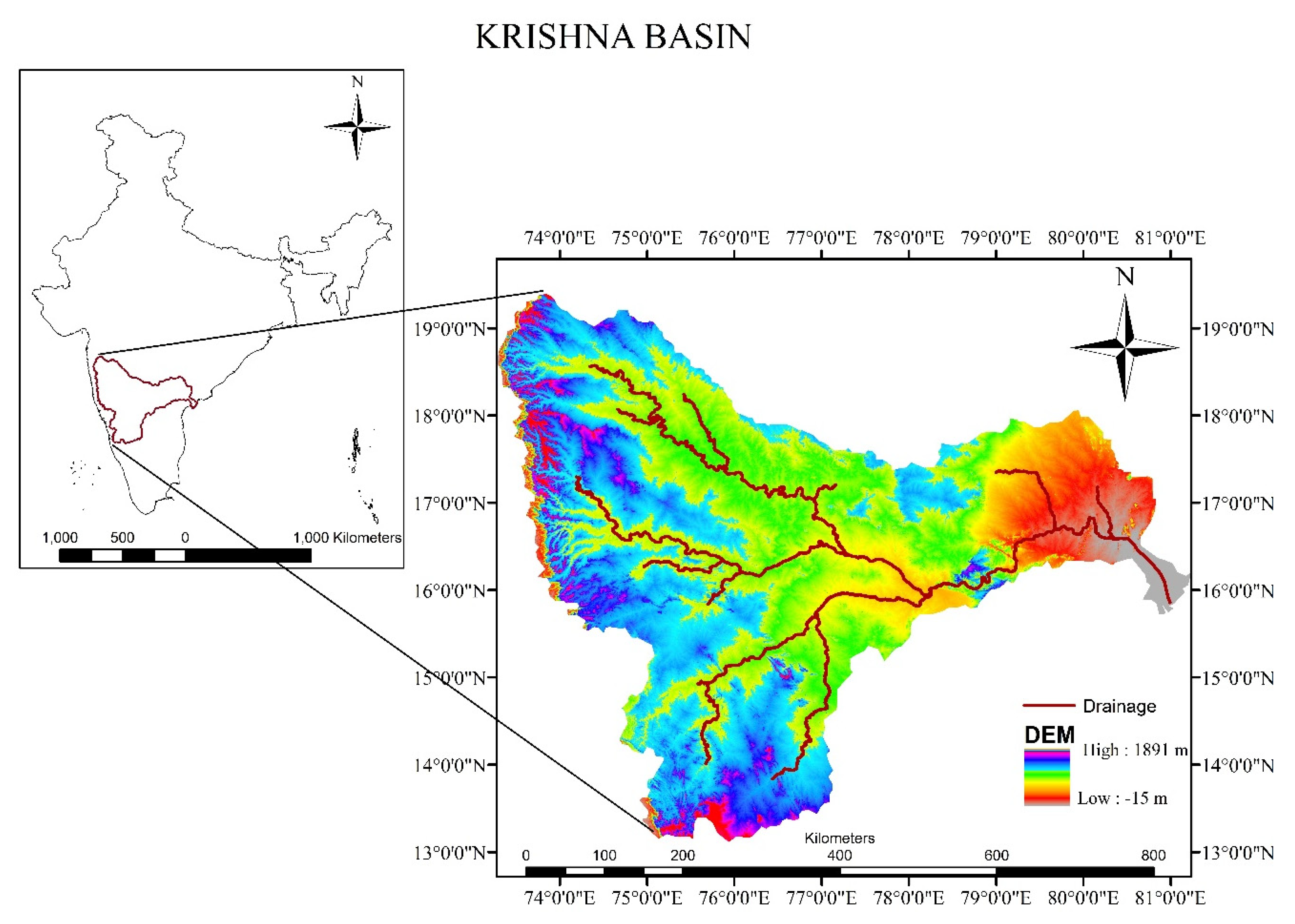
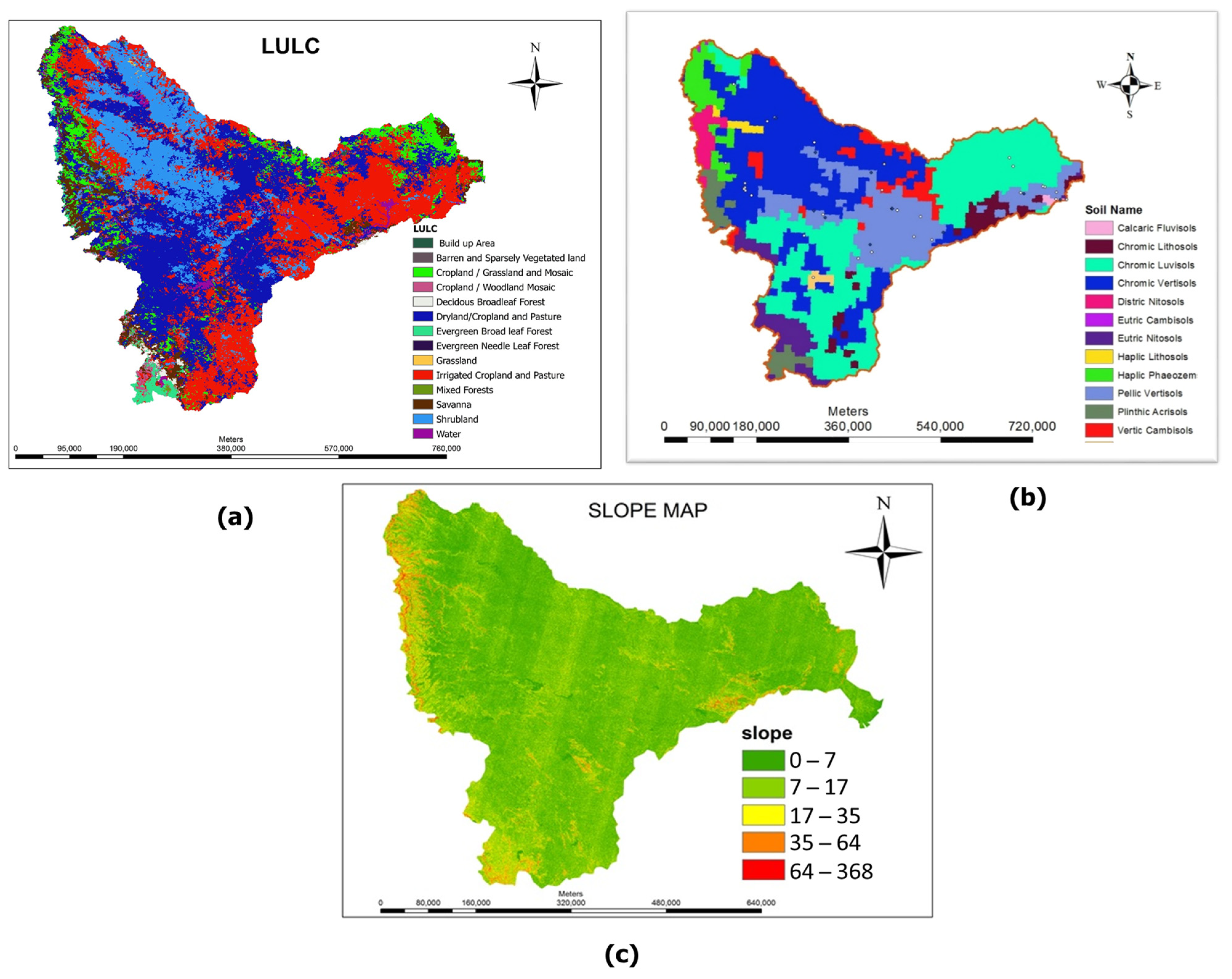
2.1. Study Area

The River Krishna basin is one of the longest rivers in central southern India, with a total surface area of 258,948 sq. km. The basin is located between 13°10′ to 19°22′ North latitudes and 73°17′ to 81°9′ East longitudes, as shown in Figure 1. It covers four Indian states: Karnataka (43.8%), Andhra Pradesh and Telangana (29.81% together), and Maharashtra (26.36%). The river has several tributaries, with Ghatprabha, Malprabha, and Tungabadhra joining on the right and Bhima, Musi, and Munneru joining on the left. The Krishna basin is divided into seven subbasins: Bhima Upper, Bhima Lower, Krishna Upper, Krishna Middle, Krishna Lower, Tungabadhra Upper, and Tungabadhra Lower.
The climate of the basin is tropical, with an average annual precipitation of 960 mm and minimum and maximum temperatures of 20.73 °C and 32.2 °C, respectively. The basin experiences varying average annual precipitation, with a maximum value of 2000 mm in the Western Ghats region and values ranging from 300 mm to 1000 mm in the delta region. Streamflow has been characterized by low flows from March to May and high flows from August to November.
The total population of the Krishna River basin was 74.2 million as per the 2011 census. Approximately 68% of the population in the basin lives in rural areas, with agriculture serving as the main source of income [56]. Approximately 77% of the total geographical area of the basin is cultivable, with the main crops identified as rice, corn, cotton, sorghum, millet, and sugar cane, along with a variety of horticulture crops. Increased population necessitates increased consumption of water for domestic and industrial purposes, putting strain on the basin’s water resources. The huge projects being developed in all states have caused interstate conflicts over water rights. According to [51], the basin is nearing closure because consumption exceeds the availability of water in the basin, which suggests the need to assess monthly changes in climate parameters and their impact on runoff when developing a water allocation policy.

2.2. Data and Methods

Table 1 lists various datasets and their resolutions. DEM estimates the basin’s minimum, maximum, and mean elevations as 18 m, 1903 m, and 518 m, respectively. Approximately 50.47% of the total area falls under the elevation zone of 500 m to 750 m. The basin is made up of 132 climate grid points measuring 50 km × 50 km, as well as 47 hydrometeorological stations.
Missing values are contributed by the streamflow data obtained from hydrometeorological stations. Due to missing stream flow data at many stations, only 14 out of 47 stations’ data were used for calibration and validation of the model. Land use information for the Krishna basin is divided into 14 categories, as shown in Figure 2a, with Agriculture (72.56%) the most important. Figure 2b represents a soil map dominated by fine-textured soil. Laterite and lateritic soils, red soils, alluvium, black soils, mixed soils (red and black, red and yellow, etc.), and alkaline and saline soils are the important soil types found in the basin. A slope map with a maximum of 5 classes based on the percentage rise was generated using DEM, as shown in Figure 2c.
Based on the availability of data, spatial and temporal variations in climate parameters and streamflow are analyzed without considering any man-made structures, such as dams, diversions, etc. The climate model data obtained from five RCMs as mentioned in Table 2 under the representative concentration pathways (RCP) 4.5 scenario and RCP 8.5 scenario are used with the assumption that emissions will be reduced by the end of the century. RCP 4.5 is a stabilization scenario in which total radiative forcing stabilizes shortly after 2100 while not exceeding the long-run radiative forcing target level [53]. RCP 8.5 is a high greenhouse gas emissions scenario that projects a significant increase in GHG emissions and concentrations over time, resulting in a radiative forcing of 8.5 W/m2 at the end of the century [54].
The SWAT model was used to simulate streamflow for the reference period using observed daily meteorological data from 1970–2005. It has a spatial resolution of 0.5° × 0.5° and includes maximum temperature (Tmax), minimum temperature (Tmin), and precipitation. The SWAT model was calibrated and validated using daily stream flow data collected from 14 gauge stations. To simulate the hydrologic characteristics for future periods using SWAT, an ensemble of high resolution past and future climate projections from regional scales—with mid-range and high-range concentration pathways of RCP 4.5 and 8.5 greenhouse gas (GHG) emissions scenario from the Centre for Climate Change Research (CCCR), Indian Institute of Tropical Meteorology, Pune, India—was obtained.
The inter-model uncertainty of climate models is estimated using the REA method, as discussed in the following sections.

2.3. Reliability Ensemble Averaging (REA)

Giorgi and Mearns (2003) [57] developed the REA method, which allows for the best estimate and reliable climate model data with a range of uncertainty. The calculation of REA follows a two-step approach: model performance and model convergence. For this study, REA is quantified using the algorithm developed by [19] for variables such as precipitation and minimum and maximum temperatures. Model performance is measured using the inverse of the Root Mean Square Error (RMSE), obtained from the Cumulative Distribution Functions (CDF) deviations between observed and simulated values for the period 1975–2005. Uncertainty in RCM’s future data is quantified using the model convergence approach, which considers the CDF deviations between individual RCMs and the weighted mean CDF derived from the model performance approach. In REA, initial weights (Equation (2)) are calculated based on the RCM’s ability to simulate historical observations in terms of root mean square error (RMSE) (Equation (1)), which indicates the model performance criteria.
RMSE = [ 1 N i = 1 N ( Observed i   RCM i ) ] 1 2
W int = [ 1 RMSE i ] [ I = 1 n 1 RMSE i ]
The following are the steps used to quantify the reliability of the climate model and to obtain the reliability ensemble mean:
  • Divide the total range of RCM variable data into 10 equal intervals of CDF with respect to the observed time series data and compute the RMSE. Inverse values of RMSE are considered as the proportional weights, and the sum of the weights of all RCMs is equal to one. Higher weights are assigned to models that perform better.
  • Model convergence criteria are applied by considering the weights obtained from model performance criteria as the initial weight for their respective RCMs.
  • The product of the initial weight (Wint) and the corresponding CDF of the future simulated with RCM (FRCMi) is taken as the weighted mean CDF (Fwm):
F wm = i W int ( i )   x   F RCM i  
  • The same procedure is repeated again as in Step 1, but the RMSE calculated with respect to the weighted CDF and future projection of RCM and weights obtained will be used in the next iteration for the respective RCMs, and a new weighted CDF with different weights is computed.
  • Repeat Steps 2 to 4 until the same weight repeats and the model convergence criteria is met.
This procedure is adapted to all grid points and three meteorological variables, such as precipitation and minimum and maximum temperatures, under the RCP 4.5 and 8.5 scenarios in the study area due to the varied nature of RCMs for the different grids and climate variables. The ensemble average of the climate variables for a particular grid is calculated using the weighted sum of the product of corresponding final weights with the respective meteorological variables. Thus, an ensemble weighted average of each climate variable is given as input to the distributed hydrological model for each grid instead of providing each RCM input separately. The minimum and maximum temperatures of the climate model data projects values that are similar to the observed data. The REA precipitation has additional bias, which is reduced by adopting the non-parametric quantile mapping method described in the following section.

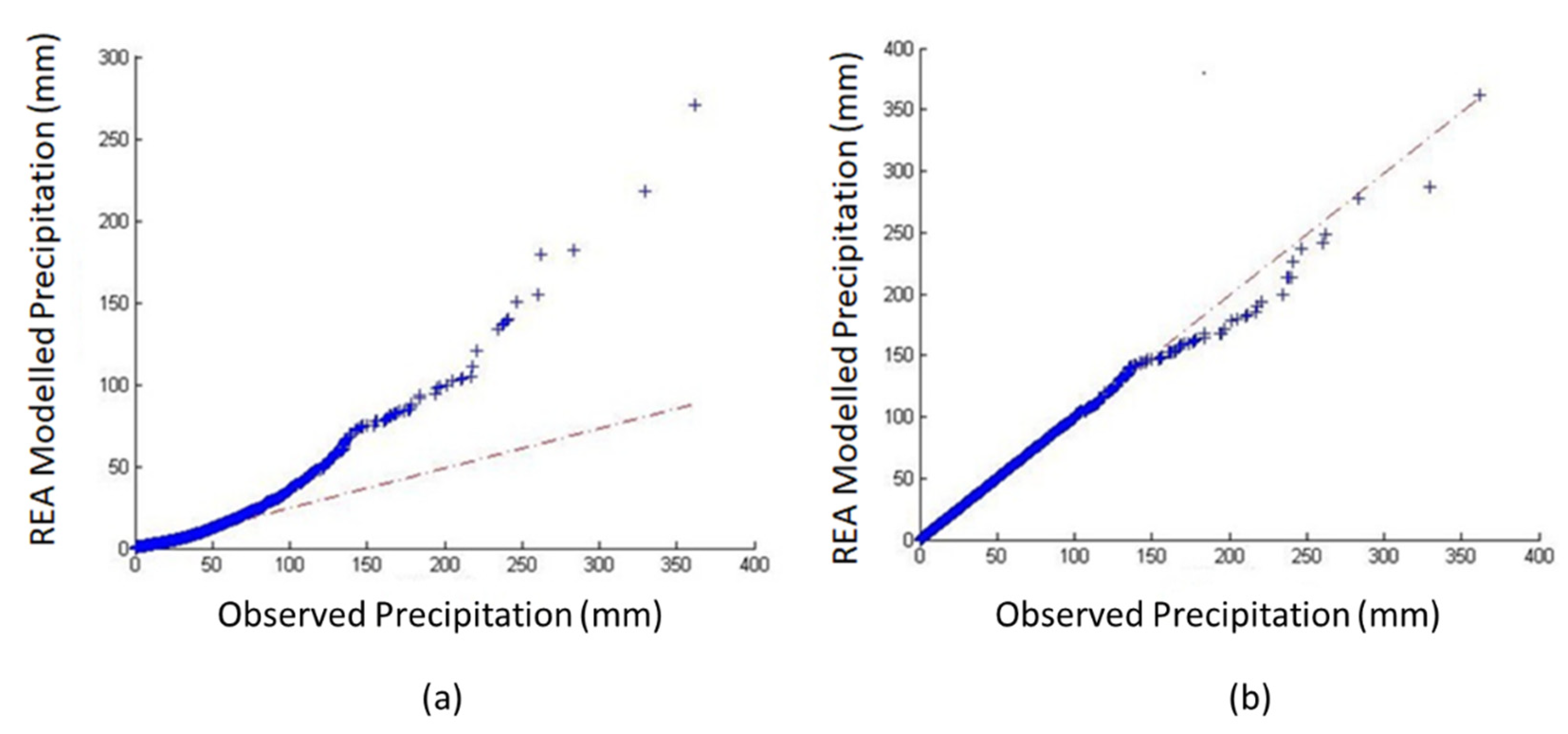
2.4. Quantile Mapping Method of Bias Correction

Quantile mapping is the most used bias correction technique due to its ease of handling large amounts of data and its computational efficiency [58,59]. The statistical bias correction used for ensemble precipitation obtained from the REA method was equal distance-based quantile-to-quantile matching. For a given variable, the CDF of REA data is first matched with the CDF of observations, resulting in the generation of a correction function based on the quantile. Then, this correction function is used to remove bias from the REA data quantile by quantile (Figure 3).

2.5. SWAT Model Setup

SWAT is a physically based, semi-distributed, and continuous process-based model that is used to simulate the rainfall–runoff process. It also predicts the hydrological impacts of climate change on water resources. The model was built using geospatial data (DEM, land use, soil and slope maps) and the hydrometeorological data. The watershed was divided into 50 subbasins with a threshold area of 60,000 sq km, and the subbasins were further divided into 898 hydrological response units (HRUs) based on 5, 10, and 10 threshold values for land use, soil type, and slope class of the watershed, respectively. As land use plays a major role in simulating the surface runoff, land use with less than 5% is eliminated. While determining HRUs of the basin, 10% of the soil and slope classes in the subbasin is eliminated. The increased number of subbasins and HRUs helps in projecting the variability of the watershed spatially. The observed meteorological data from 1970 to 2005 were used to simulate the streamflow, with a warm up period of 5 years. The calibration and validation of the model were carried out with SWAT-CUP.

2.6. Calibration and Validation of the Model Using SWAT-CUP

Uncertainties caused by input data, model structures, and parameters can be reduced using SWAT’s calibration and uncertainty programs. The model was calibrated and validated using SUFI-2, which aims to cover the most measured data with the smallest uncertainty bands. It can map the uncertainties of parameter ranges and propose the 95% prediction uncertainty (95PPU), which helps in evaluating overall uncertainty in the hydrologic response output. The model performance was evaluated using the R2, Nash–Sutcliff Efficiency (NSE) and Percent bias (PBias). The ranges of R2 and NSE are 0 and 1, respectively, with a value close to 1 indicating high model performance and efficiency. The low-magnitude values of PBias indicate better simulations, with an optimum value as 0. Positive values indicate underestimation of the model, while negative values indicate overestimation of the model.
Monthly streamflow data from 1975 to 1990 were used to calibrate the model, and data from 1991 to 2003 were used to validate it. Streamflow is generated by the summation of variables, such as base flow, interflow, and surface runoff. The parameters responsible for these variables were used against monthly streamflow data from five gauge stations. Previous studies, as well as the minimum and maximum parameter ranges established by the SWAT user guide, are used for the calibration of the Krishna River basin. SUFI-2 was used to set up the 15-parameter combinations for each iteration, and the SWAT simulation for each combination of approximately 500 iterations generated the uncertainty measures and goodness of fit by establishing new parameter ranges. The calibration process was repeated until acceptable statistics of goodness of fit were generated. The final parameter ranges obtained were used for model validation. The uncertainty in the measured streamflow was accounted for by including the estimated error of 10%. The statistical indices used for evaluating the model simulation and predictability are the coefficient of determination (R2), Nash–Sutcliff Efficiency (NSE), and Percent Bias (PBias).

2.7. Statistical Methods

For each basin, statistically significant trends in annual streamflow were determined using the Mann–Kendall’s (M-K) tau non-parametric test. If the probability value is less than or equal to 0.10, i.e., Kendall’s tau value equals zero, the trend was considered to be statistically significant. The degree of correspondence between two variables x and y, where x represents time and y represents streamflow, was calculated using Kendall’s tau. If τ = 1, then the data shows perfect positive correlation; if τ = −1, then the data exhibits perfect negative correlation; and τ = 0 shows no correlation between the pairs. Thus, a positive value of τ represents an increase in trend, while a negative value of τ represents a decrease in trend. The magnitude of the trend was estimated using Sen’s method [60,61,62].

3. Results and Discusion

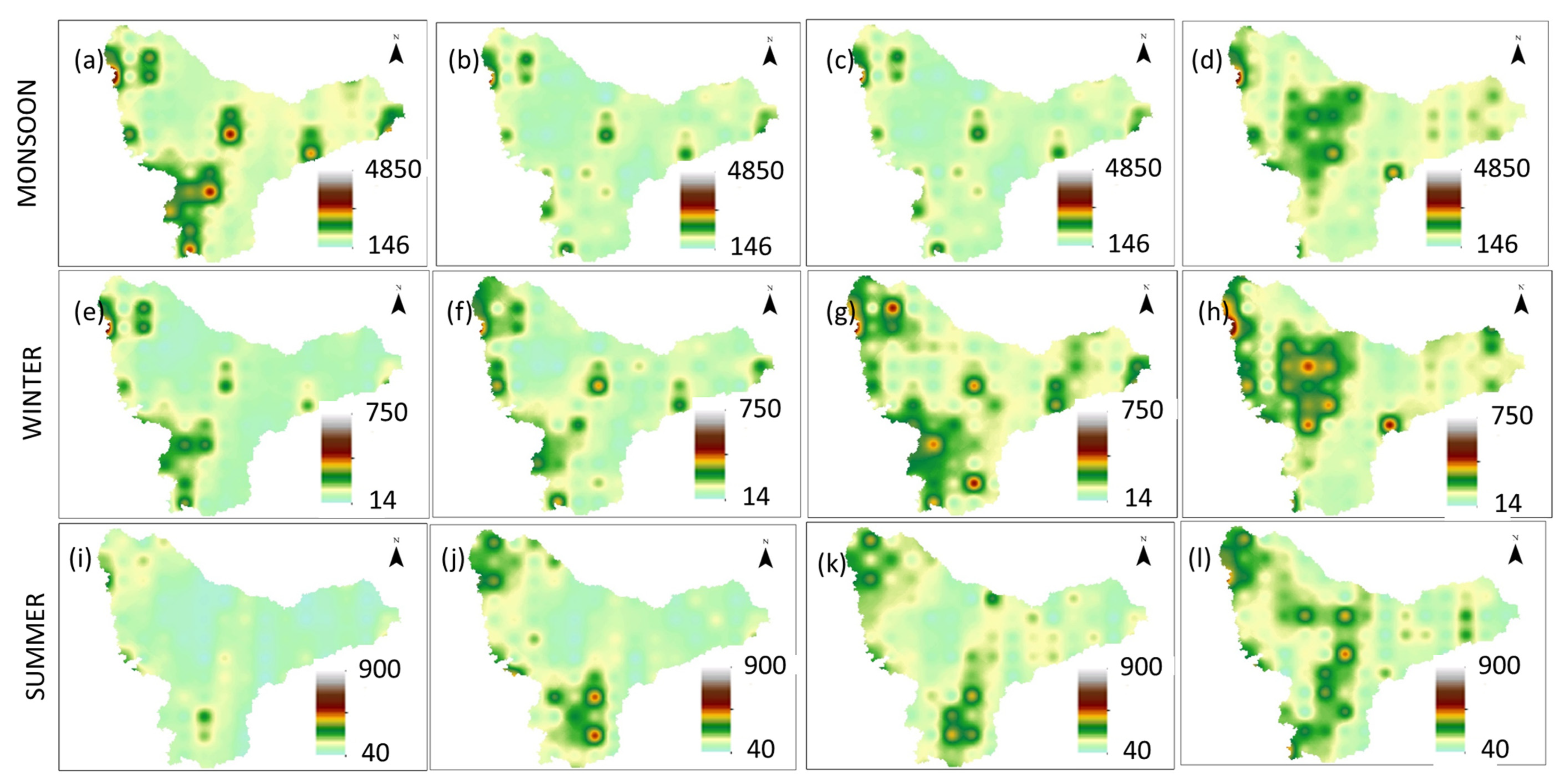
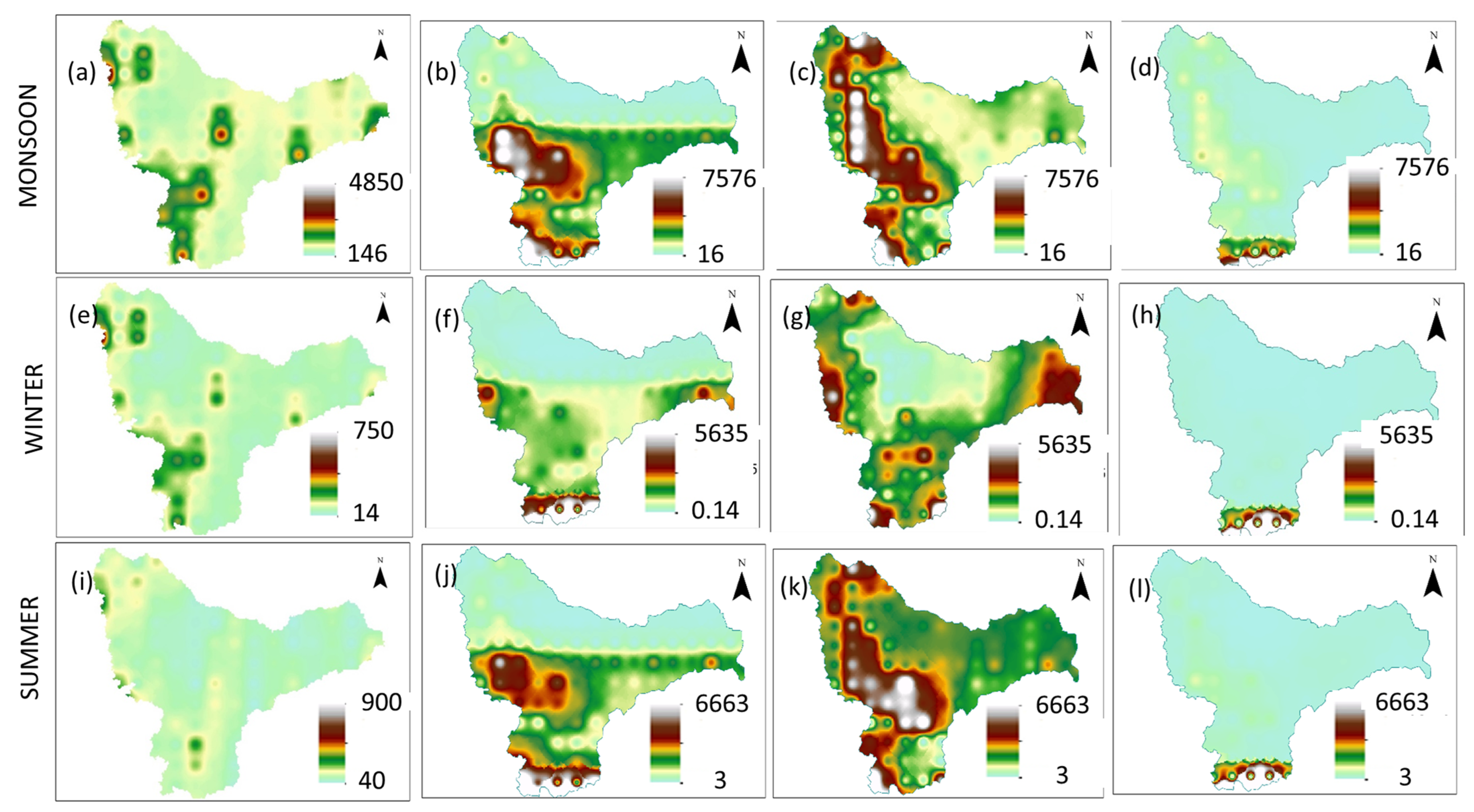
3.1. Future Projections of REA Climate Data

The observed and simulated REA precipitation and maximum and minimum temperatures are compared before and after bias correction. The results show that the observed and simulated REA temperature values agreed well, and that the precipitation data projects the same after the biases are reduced using Q-Q mapping. The climate parameters obtained cover the years 1975 to 2099. The analysis divides the total period into four 25-year segments: Historic (1980–2004), Future1 (2020–2044), Future2 (2045–2069), and Future3 (2070–2094). Figure 4 depicts the annual average precipitation (in mm/year) for the historic and future periods under RCP 4.5 and 8.5 scenarios.
The annual average variations of precipitation show an increase in the western part of the basin in Future1 and a decrease in the Future2 period under RCP 4.5. Under RCP 8.5, annual average precipitation decreases by 36% in Future1, 10% in Future2, and 60% in Future3. However, Mishra and Lilhare (2016) [11] projected a continuous increasing trend of water balance components, along with rainfall and air temperature, in both the RCP 4.5 and 8.5 scenarios of CMIP5 models in the Krishna River basin. Rainfall increases approximately 8–20% under RCP 4.5 and 10–40% in the case of RCP 8.5 by the end century. Similarly, the surface runoff, streamflow, and ET were projected to increase of approximately 20–55%, 20–60%, and 4–9% under RCP 4.5 and 35–120%, 40–120%, and 2–8% in the case of RCP 8.5 by the end of the century. Tirupathi et al. (2018) [52] projected a decrease in rainfall under future scenarios for different climate models. In the present study, daily minimum and maximum temperatures within the basin show higher values in the Future periods as compared to the Historic period under both scenarios. The Future2 period has higher temperature values than the other two future periods. Figure 5 and Figure 6 depicts seasonal variations of precipitation, i.e., monsoon (June–September), winter (October–January), and summer (February–May), for the RCP 4.5 and 8.5 scenarios.
From Figure 5, it is observed that the spatial distribution of precipitation is uniform throughout the basin, with extreme values projected in the Bhima and Middle Krishna subbasins of the Krishna River under RCP 4.5. A seasonal shift in precipitation is also projected in the winter and summer seasons of the Bhima and Tungabadra subbasins in the Future2 period and Bhima and Middle Krishna subbasins in the Future3 period. Extreme precipitation values are observed throughout the basin for the three future periods of the RCP 8.5 scenario, while the remaining portion of the basin projects precipitation values similar to the other scenario. The number of the extreme precipitation values is reduced in the future periods of the basin under RCP 8.5 as compared to RCP 4.5. Reduced precipitation is observed in the future periods as compared to the Historic period, with increased precipitation values in the central portion of the basin of the Future3 period. Precipitation values in the winter and summer seasons of the future periods are higher than in the Historic period. This reflects the shift in the monsoon in future periods. Even extreme values are observed in the central parts of the basin as compared to the Historic period in the winter and summer seasons. The maximum temperature represents an increase in all seasons in the future periods when compared to the Historic period. There is an overall increase in precipitation and temperatures in the Future3 period in the basin.
The temporal variations of the REA climate data of the future periods compared to the Historic period projects high precipitation values from June to October in Future2 & Future3, and they are more or less similar to the values of the Historic period. Peak values are observed in June (560 mm in Historic, 410 mm in Future1, 490 mm in Future2, and 520 mm in Future3), with a minimum value of 280 mm in Future1 and a maximum value of 485 mm in Future3 is detected in July under the RCP 4.5 scenario. Extreme precipitation values under the RCP 8.5 scenario range from 757.6 mm/day (monsoon) to 563.5 mm/day (summer). Precipitation values have increased overall in all months of the Future3 period of the RCP 4.5 scenario. Minimum and maximum temperature values rise in all months of the future period. From March to May, high temperatures are expected to range from 20 °C/day to 28 °C/day for the minimum temperature and 33 °C/day to 44 °C/day for the maximum temperature. Peak values of maximum temperatures observed in April are 34 °C/day in the Historic period, 36 °C/day in the Future1 period, 42 °C/day in the Future2 period, and 44 °C/day in the Future3 period in the RCP 4.5 scenario. Under the RCP 8.5 scenario, the basin experiences an overall temperature increase of 20 to 30 °C/day.

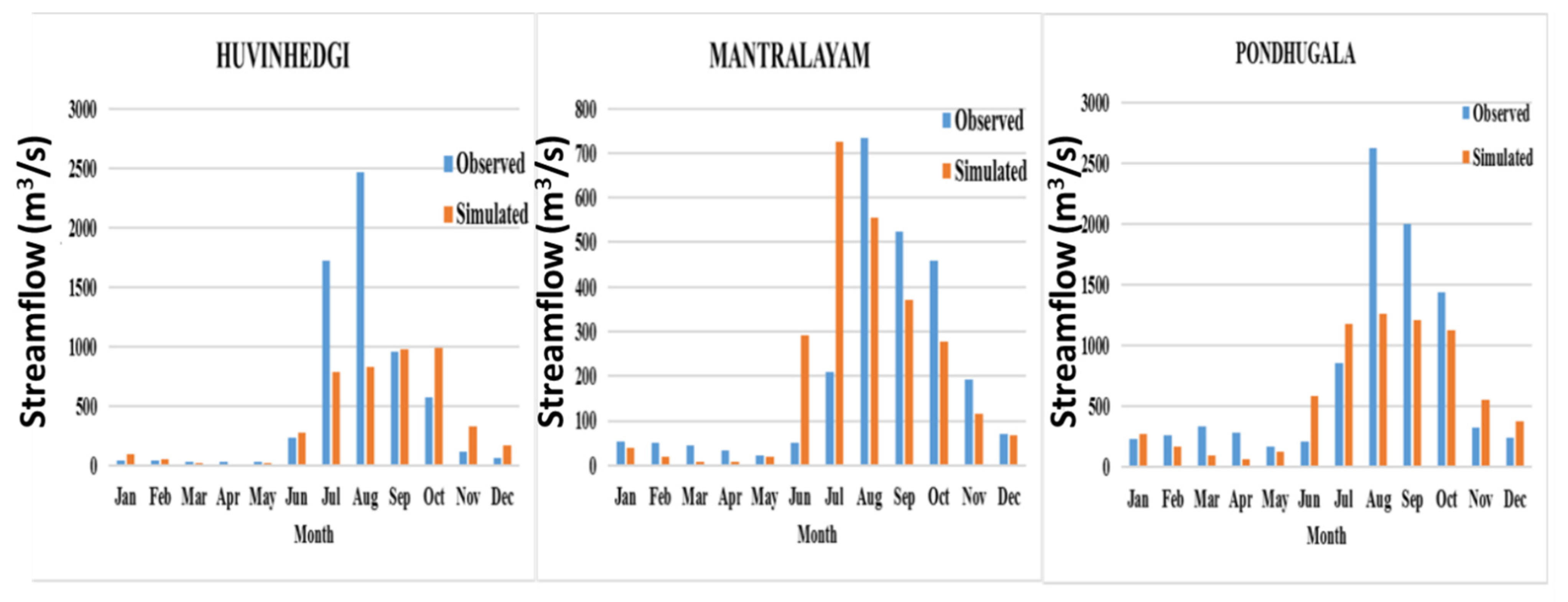
3.2. Calibration and Validation of the SWAT Model

The SUFI-2 algorithm was used to analyze the sensitivity and uncertainty of the SWAT model. For the calibration process, 15 parameters (from the SWAT-CUP manual) were chosen and used. The optimum parameter range obtained for the watershed calibration with the identical initial parameter ranges are shown in Table 3. An increase in stream flow is obtained with higher CN values and a decrease in baseflow and vice versa [63]. Whereas from Table 3, the actual CN are changed in relation to the 5% change to obtain the calibration. In this study, the rate of change of the streamflow is inconsistent with baseflow due to the change in CN values.
For example, the initial range of ESCO (Soil Evaporation Compensation Factor) is 0.4 to 0.8, but the final range is 0.94, 0.55, 0.83, 0.46, and 0.54 for the gauge stations Huvinhedgi, Narsingapur, Yadgir, Damercherla, and Keesara. The decrease in the ESCO values permits water from lower layers to upper layers to compensate the water deficit and leads to high soil evapotranspiration, thereby decreasing the surface runoff and baseflow. Thus, the changes in ESCO have a promising impact on the decreased rate in the streamflow values of the basin [64]. Table 4 represents the R2, NSE, and PBias values obtained at five gauge stations during the calibration and validation periods.
The performance of the model may suffer as a result of any combination of errors, such as geospatial data, including the land use and soil map, climate data, and the difference between the observed and simulated streamflow. However, the R2 and NSE values for the calibration range from 0.52 to 0.86 and 0.32 to 0.58, respectively, indicating that the performance was good and satisfactory during the calibration and validation periods.
The average thickness of the 95PPU band indicates the calibration strength and represents the width of the uncertainty interval, and it must be as small as possible. The 95PPU plot projects the uncertainty band generated during the calibration and validation of the model. The monthly time series of observed and simulated streamflows obtained with the fitted parameter value of the five gauge stations projects the minimum variations in streamflow dynamics over the calibration and validation periods.
Comparisons of the observed mean monthly streamflow and those produced by SWAT using REA data at three gauge stations (Figure 7)—i.e., the Huvinhedgi outlet of the Upper Bhima, Lower Bhima and Upper Krishna; the Mantralayam outlet of the Upper and Lower Tungabadhra; and the Pondhugala outlet of the Krishna River basin. The observed streamflow in July and August is more variable than the simulated streamflow at Huvinhedgi, whereas the model projects similar streamflow at Mantralayam in months other than June and July. The Pondhugala, downstream of the Huvinhedgi and Mantralayam, shows a similar pattern in mean monthly streamflow, with maximum flows in August, September, and October. The errors in the mean monthly streamflow may be due to the failure to account for reservoirs and changes in land use in the Krishna River basin.

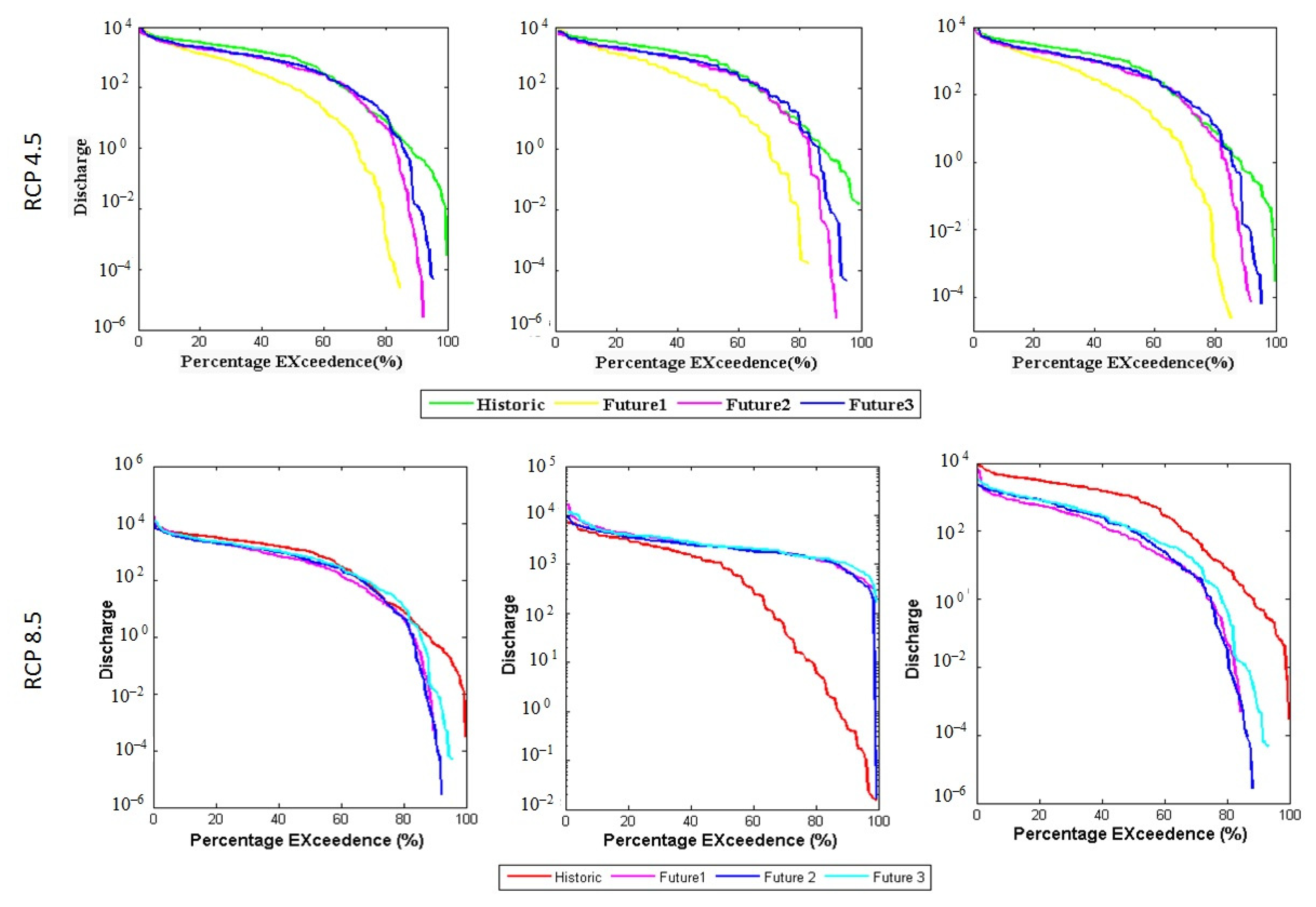
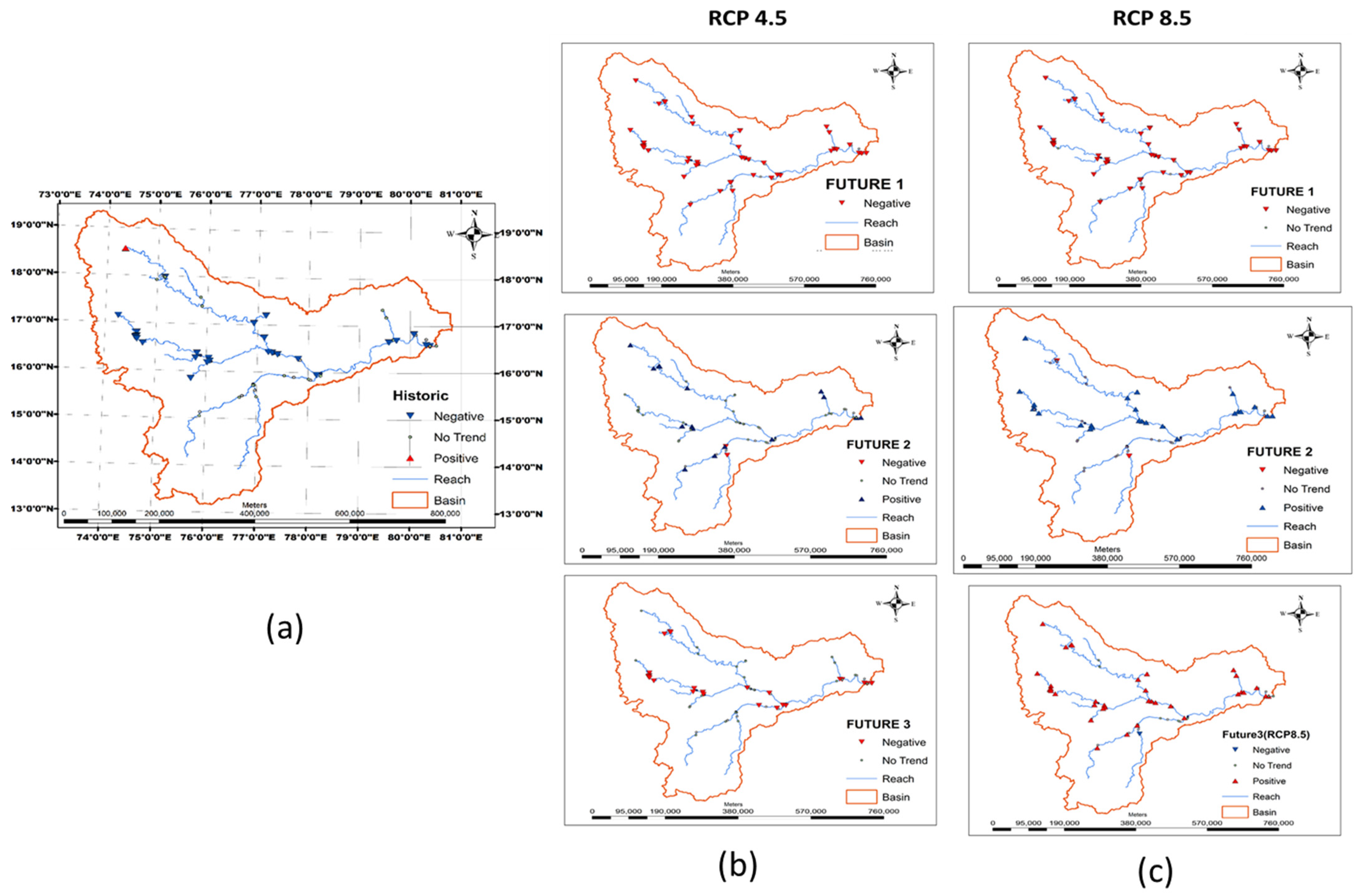
3.3. Future Streamflow Projections

According to the climate projections, lower streamflows are simulated for the future periods. Flow Duration Curves (FDCs) at three gauge stations—Huvinhedgi (Figure 8), Mantralayam (Figure 9), and Pondhugala (Figure 10)—are used to explain the relationship between the magnitude and frequency of streamflow for the future periods. These curves enumerate the flow of exceedance for a given level of probability developed on an annual, monsoon, and non-monsoon basis, assisting water managers in determining water availability in the face of climate change. Figure 8 depicts the FDC of the Huvinhedgi gauge station, representing total flows upstream of the basin, which demonstrates an overall decrease in flows during the Future1 period, with flows during theFuture2 and Future3 periods comparable to the historic period. Though Future2 and Future3 project an increase in precipitation for the basin, there is a decrease in high flows (flows that exceed 10–30% of time) and low flows are (flows that exceed 80% of time), which is mainly due to a likely increase in temperatures. The median flows (flows that exceed 30–70% of time) are similar to the Historic period flows. Both scenarios project similar patterns of curves with changes in quantity, with RCP 4.5 projecting comparatively fewer quantities than RCP 8.5.
The annual FDC of the Mantralayam and Pondhugala stations shows a decrease in high and low flows, but an increase in median flows. Flows are decreasing in the Future1 period. In the monsoon period, high flows are forecast throughout the period, with lower values in future periods compared to the Historic period. However, Nikam et al. (2018) [65] projected an increase in streamflow under the RCP 4.5 and 8.5 scenarios using IITMRegCM4-4 predictions that are calibrated and validated at single gauge stations. In the present study, the streamflows are simulated using REA climate data, which is calibrated and validated at multiple gauge stations. Many studies have even reported that the Krishna River basin is becoming more vulnerable as a result of increased human consumption of surface water resources, a reduction in surface water base flows due to over abstraction of groundwater, and fewer releases to the ocean. It also implies that hydrological changes anywhere in the basin have a negative impact on total water availability and water distribution spatially during droughts. Hence, it is important to consider water availability deficits when developing water use policies in the Krishna River basin.

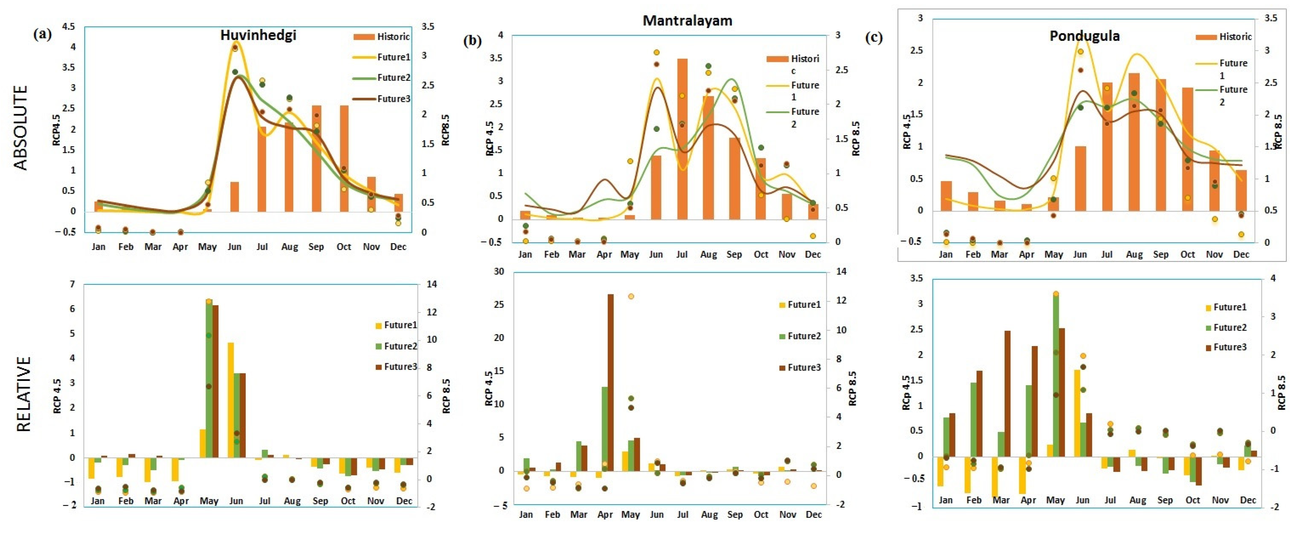
3.4. Climate Change Impact Assessment

The impact of climate change on the basin’s water resources was estimated by implementing the calibrated SWAT model with REA weather data obtained from an ensemble of five RCM for one historic and three future periods. The streamflow analysis was carried out on a monthly basis at three gauge stations: Huvinhedgi, Mantralayam, and Pondhugala. The streamflow from the Bhima subbasins was accumulated at Huvinhedgi, where Matralayam is the outlet of the Tungabadra. Streamflows from Huvinhedgi and Mantralayam meets the Pondhugala station, covering the remaining portions of the Krishna River basin. The REA precipitation data used in the SWAT model for the Krishna River subbasins (Figure 4) suggests a 20% decrease in the annual average values in the Future1 period and 4 to 6% decrease in the Future2 period, with Future3 projected to be the same as the Historic period. The monthly streamflow simulated by the SWAT model for the historic and future periods were analyzed, and the results are projected as normalized values of mean monthly flow as a ratio of annual flow. The absolute values of streamflow as the ratio of mean monthly flow and annual flow (Figure 11a) and relative change with respect to the Historic period (Figure 11b) show an increase in the Future2 and Future3 periods.
The absolute monthly flows simulated at Huvinhedgi during monsoon, winter, and summer are 716.3 m3/s, 390.5 m3/s, and 26.2 m3/s for the Historic period, whereas they are 615.65 m3/s, 100.3 m3/s, and 10.3 m3/s for the Future1 period of the RCP 4.5 scenario, and 2900.2 m3/s, 389.8 m3/s, and 259.8 m3/s are the overestimated streamflow values under the RCP 8.5 scenario. At Mantralayam and Pondhugala, the streamflows represent a decrease of about 50%, 40%, and 30% in the Future1, Future2, and Future3 periods, respectively, compared to the Historic period.
The relative change in streamflow suggests that streamflow decreases throughout the year, with an increase in June for the three gauge stations. Figure 11 shows mean monthly flow as a ratio of the mean annual flow for the historic and future periods at Huvinhedgi, Mantralayam, and Pondhugala (top: absolute values, bottom: relative change).
The Mann–Kendall Trend test was used to determine statistically significant trends in the annual streamflow of 50 subbasins obtained from the SWAT model setup. In the analysis, the MK test results of streamflow showed no trend at 21 subbasins among 50 subbasins datasets during the Historic period. However a decreasing trend at 50 and 48 subbasins is shown in the Future1 period under the RCP 4.5 and 8.5 scenarios, respectively. Increases in trend were observed at 17 subbasins in the Future2 period under RCP 4.5 and 27 subbasins under RCP 8.5, with no trend in the remaining subbasins. Furthermore, a decreasing trend in 24 subbasins was observed under RCP 4.5, with an increasing trend in 38 subbasins under RCP 8.5 of the Future3 period. The trend analysis suggests that almost all of the subbasins have a decreasing trend in both the past and the future (Table 5). Figure 12 represents positive (increase) and negative (decrease) trends at the outlets of all subbasins spatially.

4. Conclusions

In this study, future streamflows are projected using REA climate data of the RCP 4.5 and 8.5 scenarios in the SWAT Model, which is calibrated and validated at multiple gauge stations using SWAT-CUP. The REA data from the five climate models have a high correlation with the observed climate data from IMD, similar results were observed for Munneru basin which is a sub-basin for Krishna river basin [66]. The ability of the climate model data to simulate climate variables near the origin of the Krishna River basin, namely, the Western Ghats regions, is limited. The mean monthly precipitation data for the Historic period obtained from REA show less variation in the Middle Krishna, Lower Krishna, and Lower Tungabhadra. Precipitation data in the Future1 period decreased by approximately 20% when compared to the Historic period. The mean monthly flows as a ratio of the annual flow suggest a decrease in the streamflow during the Future1 period and an increase during the Future2 and Future3 periods. FDCs also suggest decreased flows in the basin, emphasizing the importance of implementing necessary changes in water use policies. Annual streamflow trends in all the 50 subbasins show a statistically significant decreasing trend in the Future1 period. No significant trends are observed in most of the subbasins in the Future2 and Future3 periods. As most of the subbasins of the Krishna River basin exhibit decreasing trends over all consecutive periods, effective adaptation and water conservation strategies are required. However, in the present study, the change in LULC is not considered for simulating streamflow for future scenarios.
Specifically, the impact of climate change on water resources of the basin is high during the Future1 period, with lower simulated streamflow. The periods from April to June have lower streamflow values in the basin. Because the basin is dominated by agricultural land, it is critical to avoid water shortage conditions through controlled usage and water management during these times. Based on the projected impacts, water resource management and adaptation strategies, such as changing cropping patterns and adapting various irrigation schemes, will be developed. Future streamflow projections based on the ensemble climate variables in this study enable decision makers to be onboard, and the projections provide them with relevant insight into possible adaptation measures.

Author Contributions

P.N.S.: Data curation, Formal analysis, Investigation, Methodology, Software, Visualization, Writing—original draft, Writing—review and editing. V.R.K.: Conceptualization, Data curation, Investigation, Methodology, Project administration, Resources, Software, Validation, Visualization, Writing—original draft, Writing—review and editing. S.M.: Conceptualization, Data curation, Investigation, Methodology, Project administration, Resources. J.D.: Software, Validation, Visualization, Writing—original draft, Writing—review and editing. V.S.: Conceptualization, Investigation, Software, Supervision, Validation, Writing—review and editing. All authors have read and agreed to the published version of the manuscript.

Funding

This research received no external funding.

Data Availability Statement

https://swat.tamu.edu/data/india-dataset/, accessed on 10 October 2022.

Acknowledgments

We acknowledge Balaji Narasimhan for providing the SWAT datasets through the Workshop materials. We are thankful to CCCR, IMD Pune for providing RCM data. The corresponding author acknowledges the support of the Virginia Agricultural Experiment Station (Blacksburg) and the Hatch Program of the National Institute of Food and Agriculture, U.S. Department of Agriculture (Washington, DC, USA).

Conflicts of Interest

The authors declare no conflict of interest.

References

  1. Satish Kumar, K.; Venkata Rathnam, E.; Sridhar, V. Tracking seasonal fluctuations of drought indices with GRACE terrestrial water storage over major river basins in South India. Sci. Total Environ. 2020, 763, 142994. [Google Scholar] [CrossRef]
  2. Sridhar, V.; Kang, H.; Ali, S.A. Human-Induced Alterations to Land Use and+ Climate and Their Responses for Hydrology and Water Management in the Mekong River Basin. Water 2019, 11, 1307. [Google Scholar] [CrossRef] [Green Version]
  3. Sridhar, V.; Jaksa, W.; Fang, B.; Lakshmi, V.; Hubbard, K.G.; Jin, X. Evaluating Bias-Corrected AMSR-E Soil Moisture using in situ Observations and Model Estimates. Vadose Zone J. 2013, 12, 1–13. [Google Scholar] [CrossRef]
  4. Field, C.B.; Barros, V.R.; Mach, K.J.; Mastrandrea, M.D.; van Aalst, M.; Adger, W.N.; Arent, D.J.; Barnett, J.; Betts, R.; Bilir, T.E.; et al. Technical summary. In Climate Change 2014: Impacts, Adaptation, and Vulnerability. Part A: Global and Sectoral Aspects. Contribution of Working Group II to the Fifth Assessment Report of the Intergovernmental Panel on Climate Change; IPCC: Geneva, Switzerland, 2014; pp. 35–94. [Google Scholar]
  5. Noble, I.R.; Huq, S.; Anokhin, Y.A.; Carmin, J.A.; Goudou, D.; Lansigan, F.P.; Osman-Elasha, B.; Villamizar, A.; Patt, A.; Takeuchi, K.; et al. Adaptation Needs and Options. Climate Change 2014 Impacts, Adaptation and Vulnerability: Part A: Global and Sectoral Aspects; IPCC: Geneva, Switzerland, 2015; pp. 833–868. [Google Scholar]
  6. Lal, M. Implications of climate change in sustained agricultural productivity in South Asia. Reg. Environ. Chang. 2011, 11 (Suppl. S1), 79–94. [Google Scholar] [CrossRef]
  7. Mukherjee, S.; Aadhar, S.; Stone, D.; Mishra, V. Increase in extreme precipitation events under anthropogenic warming in India. Weather. Clim. Extremes 2018, 20, 45–53. [Google Scholar] [CrossRef]
  8. Sujatha, E.R.; Sridhar, V. Spatial Prediction of Erosion Risk of a Small Mountainous Watershed Using RUSLE: A Case-Study of the Palar Sub-Watershed in Kodaikanal, South India. Water 2018, 10, 1608. [Google Scholar] [CrossRef] [Green Version]
  9. Sridhar, V.; Valayamkunnath, P. Land-Atmosphere Interactions in South Asia: A Regional Earth Systems Perspective: Chapter 30, Land-Atmospheric Research Applications in South and Southeast Asia; Vadrevu, K.P., Ohara, T., Justice, C., Eds.; Springer Remote Sensing/Photogrammetry: Berlin/Heidelberg, Germany, 2018; pp. 699–712. [Google Scholar] [CrossRef]
  10. Easterling, D.R.; Meehl, G.A.; Parmesan, C.; Changnon, S.A.; Karl, T.R.; Mearns, L.O. Climate Extremes: Observations, Modeling, and Impacts. Science 2019, 289, 2068–2074. [Google Scholar] [CrossRef] [PubMed] [Green Version]
  11. Mishra, V.; Lilhare, R. Hydrologic sensitivity of Indian sub-continental river basins to climate change. Glob. Planet. Chang. 2016, 139, 78–96. [Google Scholar] [CrossRef]
  12. Leon, A.S.; Kanashiro, E.A.; Valverde, R.; Sridhar, V. Dynamic Framework for Intelligent Control of River Flooding: Case Study. J. Water Resour. Plan. Manag. 2014, 140, 258–268. [Google Scholar] [CrossRef]
  13. Karl, T.R.; Meehl, G.A.; Miller, C.D.; Hassol, S.J. Weather and Climate Extremes in a Changing Climate Regions of Focus: North America, Hawaii, Caribbean, and U.S. Pacific Islands, Synthesis and Assessment Product 3.3 Report by the U.S. Climate Change Science Program and the Subcommittee on Global Change Research; IPCC: Geneva, Switzerland, 2008. [Google Scholar]
  14. Hoekema, D.J.; Sridhar, V.; Jin, X. The Adaptability and Sustainability of Surface Water Diversions Along the Main Stem of the Snake River in Southern Idaho. In Proceedings of the 2011 World Environmental and Water Resources Congress, Palm Springs, CA, USA, 22–26 May 2011. [Google Scholar]
  15. Hoekema, D.J.; Sridhar, V. Relating climatic attributes and water resources allocation: A study using surface water supply and soil moisture indices in the Snake River basin, Idaho. Water Resour. Res. 2011, 47, W07536. [Google Scholar] [CrossRef] [Green Version]
  16. Demaria, E.M.C.; Palmer, N.R.; and Roundy, K.J. Peer review report 2 on ‘Regional climate change projections of streamflow characteristics in the Northeast and Midwest. U.S.’. J. Hydrol. Reg. Stud. 2016, 5, 38–39. [Google Scholar]
  17. Chien, H.; Yeh, P.J.F.; Knouft, J.H. Modeling the potential impacts of climate change on streamflow in agricultural watersheds of the Midwestern United States. J. Hydrol. 2013, 491, 73–88. [Google Scholar] [CrossRef]
  18. Deshpande, K. Assessing Hydrological Response to Changing Climate in the Krishna Basin of India. J. Earth Sci. Clim. Change 2014, 5, 7. [Google Scholar] [CrossRef] [Green Version]
  19. Chandra, R.; Saha, U.; Mujumdar, P. Model and parameter uncertainty in IDF relationships under climate change. Adv. Water Resour. 2015, 79, 127–139. [Google Scholar] [CrossRef]
  20. Das, J.; Umamahesh, N.V. Uncertainty and Nonstationarity in Streamflow Extremes under Climate Change Scenarios over a River Basin. J. Hydrol. Eng. 2017, 22, 4017042. [Google Scholar] [CrossRef]
  21. Bejagam, V.; Keesara, V.R.; Sridhar, V. Climate change impact on water provisional service and hydropower production of Tungabhadra basin using InVEST model. River Res. Appl. 2021, 37, 9. [Google Scholar] [CrossRef]
  22. Ramabrahmam, K.; Keesara, V.R.; Srinivasan, R.; Pratap, D.; Sridhar, V. Flow Simulation and Storage Assessment in an Ungauged Irrigation Tank Cascade System Using the SWAT Model. Sustainability 2021, 13, 13158. [Google Scholar] [CrossRef]
  23. Serrão, E.A.D.O.; Silva, M.T.; Ferreira, T.R.; de Ataide, L.C.P.; Wanzeler, R.T.S.; Silva, V.D.P.R.D.; de Lima, A.M.M.; Sousa, F.D.A.S.D. Large-Scale hydrological modelling of flow and hydropower production, in a Brazilian watershed. Ecohydrol. Hydrobiol. 2020, 21, 23–35, ISSN 1642-3593. [Google Scholar] [CrossRef]
  24. de Andrade, C.W.; Montenegro, S.M.; Montenegro, A.A.; Lima, J.R.D.S.; Srinivasan, R.; Jones, C.A. Soil moisture and discharge modeling in a representative watershed in northeastern Brazil using SWAT. Ecohydrol. Hydrobiol. 2018, 19, 238–251, ISSN 1642-3593. [Google Scholar] [CrossRef]
  25. Hillard, U. Assessing snowmelt dynamics with NASA scatterometer (NSCAT) data and a hydrologic process model. Remote Sens. Environ. 2003, 86, 52–69. [Google Scholar] [CrossRef]
  26. Uniyal, B.; Jha, M.K.; Verma, A.K. Assessing Climate Change Impact on Water Balance Components of a River Basin Using SWAT Model. Water Resour. Manag. 2015, 29, 4767–4785. [Google Scholar] [CrossRef]
  27. Piras, M.; Mascaro, G.; Deidda, R.; Vivoni, E.R. Quantification of hydrologic impacts of climate change in a Mediterranean basin in Sardinia, Italy, through high-resolution simulations. Hydrol. Earth Syst. Sci. 2014, 18, 5201–5217. [Google Scholar] [CrossRef] [Green Version]
  28. Sridhar, V. Tracking the Influence of Irrigation on Land Surface Fluxes and Boundary Layer Climatology. J. Contemp. Water Res. Educ. 2013, 152, 79–93. [Google Scholar] [CrossRef]
  29. Sridhar, V.; Hubbard, K.G.; Wedin, D.A. Assessment of Soil Moisture Dynamics of the Nebraska Sandhills Using Long-Term Measurements and a Hydrology Model. J. Irrig. Drain. Eng. 2006, 132, 463–473. [Google Scholar] [CrossRef] [Green Version]
  30. Valayamkunnath, P.; Sridhar, V.; Zhao, W.; Allen, R.G. Intercomparison of surface energy fluxes, soil moisture, and evapotranspiration from eddy covariance, large-aperture scintillometer, and modeling across three ecosystems in a semiarid climate. Agric. For. Meteorol. 2018, 248, 22–47. [Google Scholar] [CrossRef]
  31. Abbaspour, K.C.; Rouholahnejad, E.; Vaghefi, S.; Srinivasan, R.; Yang, H.; Kløve, B. A continental-scale hydrology and water quality model for Europe: Calibration and uncertainty of a high-resolution large-scale SWAT model. J. Hydrol. 2015, 524, 733–752. [Google Scholar] [CrossRef] [Green Version]
  32. Abbaspour, K.C.; Yang, J.; Maximov, I.; Siber, R.; Bogner, K.; Mieleitner, J.; Zobrist, J.; Srinivasan, R. Modelling hydrology and water quality in the pre-alpine/alpine Thur watershed using SWAT. J. Hydrol. 2007, 333, 413–430. [Google Scholar] [CrossRef]
  33. Abbaspour, K.C.; Johnson, C.; van Genuchten, M.T. Estimating Uncertain Flow and Transport Parameters Using a Sequential Uncertainty Fitting Procedure. Vadose Zone J. 2004, 3, 1340. [Google Scholar] [CrossRef]
  34. Yang, J.; Reichert, P.; Abbaspour, K.C.; Xia, J.; Yang, H. Comparing uncertainty analysis techniques for a SWAT application to the Chaohe Basin in China. J. Hydrol. 2008, 358, 1–23. [Google Scholar] [CrossRef]
  35. Jha, M.; Pan, Z.; Takle, E.S.; Gu, R. Impacts of climate change on streamflow in the Upper Mississippi River Basin: A regional climate model perspective. J. Geophys. Res. Atmos. 2004, 109, D09105. [Google Scholar] [CrossRef]
  36. Bhadoriya, U.P.S.; Mishra, A.; Singh, R.; Chatterjee, C. Implications of climate change on water storage and filling time of a multipurpose reservoir in India. J. Hydrol. 2020, 590, 125542. [Google Scholar] [CrossRef]
  37. Das, J.; Treesa, A.; Umamahesh, N.V. Modelling Impacts of Climate Change on a River Basin: Analysis of Uncertainty Using REA & Possibilistic Approach. Water Resour. Manag. 2018, 32, 4833–4852. [Google Scholar] [CrossRef]
  38. Das, J.; Nanduri, U.V. Assessment and evaluation of potential climate change impact on monsoon flows using machine learning technique over Wainganga River basin, India. Hydrol. Sci. J. 2018, 63, 1020–1046. [Google Scholar] [CrossRef] [Green Version]
  39. Ghosh, S.; Raje, D.; Mujumdar, P.P. Mahanadi streamflow_climate change impacts assessment and adaptive strategies.pdf. Curr. Sci. 2010, 98, 1084–1091. [Google Scholar]
  40. Islam, A.; Sikka, A.K.; Saha, B.; Singh, A. Streamflow Response to Climate Change in the Brahmani River Basin, India. Water Resour. Manag. 2012, 26, 1409–1424. [Google Scholar] [CrossRef]
  41. Das, J.; Nanduri, U.V. Future Projection of Precipitation and Temperature Extremes Using Change Factor Method over a River Basin: Case Study. J. Hazard. Toxic Radioact. Waste 2018, 22, 04018006. [Google Scholar] [CrossRef]
  42. Gosain, A.K.; Rao, S.; Arora, A. Climate change impact assessment of water resources of {India}. Curr. Sci. 2011, 101, 356–371. [Google Scholar]
  43. Anandhi, A.; Srinivas, V.V.; Nanjundiah, R.S.; Kumar, D.N. Downscaling precipitation to river basin in India for IPCC SRES scenarios using support vector machine. Int. J. Clim. 2007, 28, 401–420. [Google Scholar] [CrossRef]
  44. Coulibaly, P.; Dibike, Y.; Anctil, F. Downscaling Precipitation and Temperature with Temporal Neural Networks. J. Hydrometeorol. 2005, 6, 483–496. [Google Scholar] [CrossRef]
  45. Das, J.; Umamahesh, N.V. Assessment of uncertainty in estimating future flood return levels under climate change. Nat. Hazards 2018, 93, 109–124. [Google Scholar] [CrossRef]
  46. Mujumdar, P.P.; Ghosh, S. Modeling GCM and scenario uncertainty using a possibilistic approach: Application to the Mahanadi River, India. Water Resour. Res. 2008, 44, W06407. [Google Scholar] [CrossRef]
  47. Bouwer, L.M.; Aerts, J.C.J.H.; Droogers, P.; Dolman, A.J. Detecting the long-term impacts from climate variability and increasing water consumption on runo ff in the Krishna river basin (India). Hydrol. Earth Syst. Sci. 2006, 10, 1249–1280. [Google Scholar] [CrossRef]
  48. Gosain, A.K.; Rao, S.; Basuray, D. Climate change impact assessment on hydrology of Indian river basins. Current 2006, 90, 346–353. [Google Scholar]
  49. Amarasinghe, U.; Sharma, B.R.; Aloysius, N.; Scott, C.; Smakhtin, V.; De Fraiture, C. Spatial Variation in Water Supply and Demand across River Basins of India; International Water Management Institute: Colombo, Sri Lanka, 2004; Volume 83. [Google Scholar]
  50. Amarasinghe, U.A.; Shah, T.; Turral, H.; Anand, B.K. India’s Water Future to 2025–2050: Business-as-Usual Scenario and Deviations; IWMI: Colombo, Sri Lanka, 2007. [Google Scholar]
  51. Biggs, T.W.; Gaur, A.; Scott, C.; Thenkabail, P.S.; Rao, P.G.; Gumma, M.K.; Acharya, S.; Turral, H.N. Closing of the Krishna Basin: Irrigation, Streamflow Depletion and Macroscale Hydrology; IWMI: Colombo, Sri Lanka, 2007. [Google Scholar]
  52. Chanapathi, T.; Thatikonda, S.; Raghavan, S. Analysis of rainfall extremes and water yield of Krishna river basin under future climate scenarios. J. Hydrol. Reg. Stud. 2018, 19, 287–306. [Google Scholar] [CrossRef]
  53. Thomson, A.M.; Calvin, K.V.; Smith, S.J.; Kyle, G.P.; Volke, A.; Patel, P.; Delgado-Arias, S.; Bond-Lamberty, B.; Wise, M.A.; Clarke, L.E.; et al. RCP 4.5: A pathway for stabilization of radiative forcing by 2100. Clim. Chang. 2011, 109, 77–94. [Google Scholar] [CrossRef] [Green Version]
  54. Riahi, K.; Rao, S.; Krey, V.; Cho, C.; Chirkov, V.; Fischer, G.; Kindermann, G.; Nakicenovic, N.; Rafaj, P. RCP 8.5—A scenario of comparatively high greenhouse gas emissions. Clim. Chang. 2011, 109, 33. [Google Scholar] [CrossRef] [Green Version]
  55. Sowjanya, P.N.; Venkata Reddy, K.; Shashi, M. Intra- and interannual streamflow variations of Wardha watershed under changing climate. ISH J. Hydraul. Eng. 2020, 26, 197–208. [Google Scholar] [CrossRef]
  56. Sarma, J. Impact of High Rinfall/Floods on Groundwater Resources in the Krishna River Basin (during 1999–2009); India Environment Portal: New Delhi, India, 2011. [Google Scholar]
  57. Giorgi, F.; Mearns, L.O. Probability of regional climate change based on the Reliability Ensemble Averaging (REA) method. Geophys. Res. Lett. 2003, 30, 2–5. [Google Scholar] [CrossRef]
  58. Gudmundsson, L.; Bremnes, J.B.; Haugen, J.E.; Engen-Skaugen, T. Technical Note: Downscaling RCM precipitation to the station scale using statistical transformations—A comparison of methods. Hydrol. Earth Syst. Sci. 2012, 16, 3383–3390. [Google Scholar] [CrossRef] [Green Version]
  59. Piani, C.; Haerter, J.O.; Coppola, E. Statistical bias correction for daily precipitation in regional climate models over Europe. Theor. Appl. Clim. 2009, 99, 187–192. [Google Scholar] [CrossRef] [Green Version]
  60. Mann, H.B. Nonparametric Tests Against Trend Author(s): Henry B. Mann Published by: The Econometric Society Stable URL: http://www.jstor.org/stable/1907187 REFERENCES Linked references are available on JSTOR for this article: You may need to log in to JSTOR t. J. Econom. Soc. 2016, 13, 245–259. [Google Scholar] [CrossRef]
  61. Nayak, P.C.; Wardlaw, R.; Kharya, A.K. Water balance approach to study the effect of climate change on groundwater storage for Sirhind command area in India. Int. J. River Basin Manag. 2015, 13, 243–261. [Google Scholar] [CrossRef]
  62. Hamed, K.H.; Rao, A.R. A modified Mann-Kendall trend test for autocorrelated data. J. Hydrol. 1998, 204, 182–196. [Google Scholar] [CrossRef]
  63. Singh, L.; Saravanan, S. Simulation of monthly streamflow using the SWAT model of the Ib River watershed, India. J. Hydro-Environ. Res. 2020, 3, 95–105. [Google Scholar] [CrossRef]
  64. Jha, M.K. Evaluating Hydrologic Response of an Agricultural Watershed for Watershed Analysis. Water 2011, 3, 604–617. [Google Scholar] [CrossRef] [Green Version]
  65. Nikam, B.R.; Garg, V.; Jeyaprakash, K.; Gupta, P.K.; Srivastav, S.K.; Thakur, P.K.; Aggarwal, S.P. Analyzing future water availability and hydrological extremes in the Krishna basin under changing climatic conditions. Arab. J. Geosci. 2018, 11, 581. [Google Scholar] [CrossRef]
  66. Buri, E.S.; Keesara, V.R.; Loukika, K.N.; Sridhar, V. Spatio-Temporal Analysis of Climatic Variables in the Munneru River Basin, India, Using NEX-GDDP Data and the REA Approach. Sustainability 2022, 14, 1715. [Google Scholar] [CrossRef]
Figure 1. Location map of the Krishna River basin.
Climate 10 00190 g001
Figure 2. Thematic maps of the Krishna basin (a) Land use/Land cover, (b) Soil and (c) Slope.
Climate 10 00190 g002
Figure 3. Quantile–Quantile (QQ) map of observed vs. REA modelled precipitation data (a) Before bias correction (b) After bias correction.
Climate 10 00190 g003
Figure 4. Annual average precipitation variation in the Krishna basin for (a) Historic, Future1 (b,e), Future2 (c,f), and Future3 (d,g) periods under RCP 4.5 and RCP 8.5 scenarios.
Climate 10 00190 g004
Figure 5. Seasonal average precipitation variation in the Krishna basin for Historic, Future1, Future2, and Future3 periods of Monsoon (ad), winter (eh) and summer (il) under the RCP 4.5 scenarios.
Climate 10 00190 g005
Figure 6. Seasonal average precipitation variation in the Krishna basin for Historic, Future1, Future2, and Future3 periods of Monsoon (ad), winter (eh) and summer (il) under the RCP 8.5 scenario.
Climate 10 00190 g006
Figure 7. Observed and SWAT-simulated streamflow at three gauge stations for the Historic period (1975–2005).
Climate 10 00190 g007
Figure 8. Annual, monsoon, and non-monsoon flow duration curves at the Huvinhedgi gauge station for historic and future periods under RCP 4.5 and RCP 8.5 scenarios.
Climate 10 00190 g008
Figure 9. Annual, monsoon, and non-monsoon flow duration curves at the Mantralayam gauge station for historic and future periods under RCP 4.5 and RCP 8.5 scenarios.
Climate 10 00190 g009
Figure 10. Annual, monsoon, and non-monsoon flow duration curves at the Pondhugala gauge station for historic and future periods under RCP 4.5 and RCP 8.5 scenarios.
Climate 10 00190 g010
Figure 11. Mean monthly flow as a ratio of mean annual flow for historic and future periods of RCP 4.5 (line plot) and RCP 8.5 (dotty plot) at (a) Huvinhedgi, (b) Mantralayam, and (c) Pondhugula (top: absolute values, bottom: relative change).
Climate 10 00190 g011
Figure 12. Annual streamflow trends (a) historic, (b) RCP 4.5 scenario, (c) RCP 8.5 scenario.
Climate 10 00190 g012
Table 1. Description and source of hydro geospatial and climatological database.
Data TypeResolutionSource
Digital Elevation Model30 mAdvanced Space borne Thermal Emission and Reflection Radiometer (ASTER),
Land use/Land cover400 mhttps://swat.tamu.edu/data/india-dataset/, accessed on 15 March 2019
Soil1:5,000,000https://swat.tamu.edu/data/india-dataset/, accessed on 15 March 2019
Observed Climate data0.5° gridIndian Meteorological Department, Pune.
Climate Model data0.5° gridCentre for Climate Change Research (CCCR), Indian Institute of Meteorology (IITM) Pune. ftp://cccr.tropmet.res.in/iRODS_DATA/CORDEX-Data, accessed on 23 May 2017
River Discharge14 stationsCentral Water Commission (CWC)
Table 2. Details of RCM models.
AcronymRCPFull Name
ACCESS4.58.5Australian Community Climate and Earth System Simulator
CCSM44.58.5Community Climate System Model
CNRM_CM54.58.5Centre National de Recherché Meteorologiques
NorESM 14.58.5Norwegian Earth System Model 1
MPI-ESM-LR4.5-Max Plank Institute Earth System Model
Table 3. Calibration parameter ranges for the five-gauge stations.
S.NoParameterInitial FinalHuvinhedgiNarsingpurYadgirDamercherlaKeesara
1R__CN2.mgt−0.200.20−0.190.030.05−0.170.17
2V__ALPHA_BF.gw01.000.200.960.950.160.26
3V__GW_DELAY.gw050027545427414352
4V__GWQMN.gw050001.241.751.7010501100
5V__GW_REVAP.gw0.020.200.190.190.170.160.14
6R__SOL_K(..).sol0.140.990.990.370.660.550.72
7R__SOL_AWC(..).sol−0.150.600.040.550.290.340.42
8R__SOL_BD(..).sol0.050.700.690.120.670.610.58
9V__ALPHA_BNK.rte0.001.000.600.400.430.360.65
10V__CH_N2.rte−0.090.090.090.110.080.070.04
11V__CH_K2.rte18.72103.9688.3686.7547.4548.4253.26
12V__ESCO.hru01.000.940.550.830.460.62
13R__EPCO.hru01.000.300.590.160.510.48
14R__SLSUBBSN.hru−0.120.300.130.09−0.050.250.06
Where V__ represents that existing parameter, value is to be replaced by the given value and R__ represents that existing parameter value to be multiplied by (1+ a given value). Bold values representing the sensitive param.
Table 4. Goodness of fit parameters for calibration and validation periods.
Stream Gauge StationCalibrationValidation
R2NSEPBiasR2NSEPBias
Huvinhedgi0.620.62−13.500.420.4279.80
Narsingapur0.620.52−41.900.500.47−73.50
Yadgir0.860.58−27.100.400.32−88.50
Damercherla0.800.75−8.350.580.43−57.80
Keesara0.680.62−12.400.520.4865.40
Table 5. Number of subbasins with increasing or decreasing trend.
Climate PeriodRCP 4.5RCP 8.5
IncreasingDecreasingIncreasingDecreasing
Historic128
Future I-50-48
Future II172272
Future III-24381
Publisher’s Note: MDPI stays neutral with regard to jurisdictional claims in published maps and institutional affiliations.

