A New Way to Obtain Climate Files in Areas with the Presence of Microclimates by Applying the Sandia Method: A Galician Case Study

Abstract

In order to obtain reliable energy simulation results, it is essential to have accurate climate files corresponding to specific geographical locations. The present work describes a selection process of the Typical Meteorological Months (TMM) that will generate the Typical Meteorological Years (TMY) in eight locations of the Community of Galicia for an analysis period between 2008 and 2017 (10 years). The region of Galicia, located in the northwest of the Iberian Peninsula, due to its particular orography, is prone to the generation of differentiated microclimates in relatively close locations. The process of selecting the typical meteorological months has been carried out following the Sandia Laboratories method. In the present work, data from terrestrial meteorological stations have been combined with solar radiation data obtained from satellite images. Finally, for the validation and comparative study of results, files have been generated in Energy Plus Weather (epw) format. Trends have been checked and typical statistics have been used to analyse the correlations between the files generated with the Sandia method, and the usual reference files (LT, WY, BY). It is observed that with the eight files generated, new differentiated climates are detected, which will affect the improvement of the precision of the energy simulations of buildings that are going to be carried out. For example, in the case of the Campus Lugo and Pedro Murias stations, located in the same climatic zone according to Spanish regulations, differences are observed in the annual averages: DTm (13.7%), WV (41%) or GHI (9%).

1. Introduction

Building energy simulation programs (BES, Building Energy Simulation) are among the most used tools to help reduce energy consumption. These techniques are used both in the design phases of the building and installations, as well as in the exploitation phase.

The objective of an energy simulation is to obtain the global thermal performance of a building, which will be a function of several factors: their geographical location and orientation, the composition of its envelope, the type and size of its thermal installations and at last, the level occupation (schedules, number of people, type of consumption). Three of the four points indicated: climatic profile, envelope and dimensioning of thermal installations are directly influenced by the climatology of the area where the building is located. Therefore, it is essential to have accurate data of the climatic profiles corresponding to its geographical location in order to obtain reliable results from the energy simulation and thus be able to make the most appropriate decision for the proposed purpose, which is to try to reduce energy consumption and CO₂ emissions into the atmosphere.

Associated with the geographical area of Galicia (northwest of the Iberian Peninsula) there are currently six officially available climate files that correspond to the climatic zones defined by the Technical Building Code of Spain [1], suitable for being used with simulation programs that use calculation engines: Energy Plus^® [2], DOE 2.2^®. These files are aimed at carrying out the energy certification of buildings, but they are not valid in principle to carry out detailed energy simulations for a certain geographical location, for which reason the creation of new files with real data from the region is justified, to reflect the climatic variety present in it.

There is a variety of widely contrasted methods that can be used to determine the 12 TMM that allow the elaboration of climatic files, necessary for the energy simulation of buildings [3,4,5,6,7,8,9,10,11,12].

The main issue addressed in this research is the insufficient precision of the energy simulations carried out in the building sector in Galicia due to the fact that the set of climatic files available for this purpose does not collect the climatic singularity with sufficient precision [13].

The purpose of this paper is to describe the process of preparing a series of 8 climatic files, following the Sandia National Laboratories method [3], with the particularity that it must highlight the aforementioned existing climatic diversity.

Following what has been indicated, the first step to generating the climatic files will be the geographical and climatology study of the area.

Geographical and Climatological Description of the Region

The region of Galicia (Spain), located in the northernmost part of the Iberian Peninsula, stands out to the west in the southern part of Atlantic Europe. Its most extreme coordinates are located between 41.8° and 43.75° North latitude and 6.73° and 9.29° West longitude. Its total area is 29,574 km² and it is politically divided into four provinces: La Coruña, Lugo, Orense and Pontevedra. It limits to the West with the Atlantic Ocean and to the North with the Cantabrian Sea.

It is a not very extensive region: 29,574 km² (11,419 square miles). In its orography, a coastal relief in a strip of 1600 km, and an elevated interior with low and blunt mountains can be highlighted. In certain areas, rugged slopes arise, such as in the Sil canyons or the high mountain areas of Lugo and Orense, with peaks of more than 2000 m above sea level. The orography described, combined with the existence of a multitude of rivers, contributes to the formation of a set of microclimates, with strong variations in areas with little more than 200 km², which in turn can undergo alterations from one to another season of the year https://es.qaz.wiki/wiki/Galicia_(Spain) (accessed on 1 September 2022).

Galicia’s climate is oceanic, generally temperate and humid (due to the Atlantic influence), but highly variable throughout the year. In its southern area, the climate is similar to the Mediterranean, as there is a period (July and August) in which drought situations take place [14].

According to the Koppen scale, Galicia is classified among those of type Cfb for the north and high mountain areas, Csa in the south and Csb in the rest of the region (central and coastal zone) [15].

2. Materials and Methods

The Typical Meteorological Year (TMY) representative of a period of time is constituted by the concatenation of the 12 Typical Meteorological Months (TMM) representative of said period.

In the present work, it was decided to apply the Sandia method [3,16] because it is one of the most widely used and recognized methods. The period of time under study covers from 2008 to 2017 (10 years) due to the availability of data on the climatic parameters for the selected terrestrial meteorological stations.

The process begins by means of an individual exam for every month of each year and selecting the most typical of those that occupy the same position in the successive years of the indicated period. This is a comparison process that is repeated 12 times. Finally, the twelve selected representative months are concatenated to obtain the Typical Meteorological Year. In order to avoid discontinuities between consecutive months, a smoothing of the data of each parameter has been carried out during the last 6 h of each month and the following 6 of the following month [16]; other methods use 8 h [7,9]. To carry out the study, the script proposed in [16,17,18] has been followed.

The selection of each of the 12 Typical Meteorological Months is based on the analysis of nine daily indices: Daily mean dry temperature (DTm), Daily maximum dry temperature (DTmax), Daily minimum dry temperature (TDmin), Daily mean dew point temperature (DPm), Daily maximum dew point temperature (DPmax), Daily minimum dew point temperature (DPmin), Daily mean wind velocity (WVm), Daily maximum wind velocity (WVmax) and Daily mean horizontal global radiation (GHR).

2.1. Data Sources Used

In order to carry out this analysis, data from MeteoGalicia (network of terrestrial meteorological stations of the Autonomous Community of Galicia) have been used due to the greater availability of data and spatial coverage compared to AEMET (State Meteorological Agency from Spain).

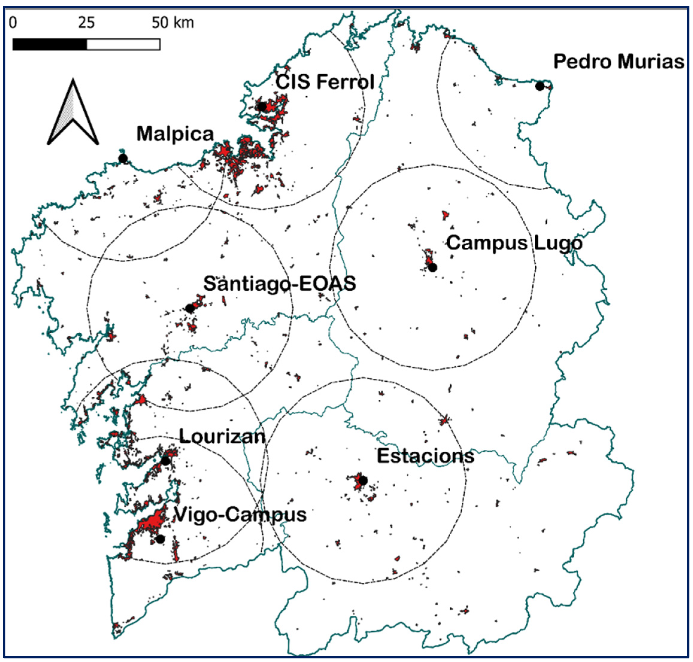
Currently, the network of MeteoGalicia stations has more than 160 stations distributed throughout the community, but only 43 of them meet the required conditions: both regarding the available climatic indices and in relation to the amplitude of the history of data stored (period from 2008 to 2017). Finally, for the present work, eight stations have been selected applying the criterion of proximity to the most populated areas of the region (

Table 1. Geographical situation of the selected stations.

Province	Station	Lat [N] WGS84 (EPSG:4326)	Long [E] WGS84 (EPSG:4326)	Altitude (m.s.n.m)	Sea Distance (Km)	Climatic Zone 1
A Coruña	CIS Ferrol	43.492	−0.2523	37	1	C1
A Coruña	Malpica	43.336	−8.8364	161	1	C1
A Coruña	Santiago-EOAS	42.876	−8.5594	255	40	D1
Lugo	Campus Lugo	42.993	−7.5469	400	90	D1
Lugo	Pedro Murias	43.541	−7.0830	51	1	D1
Ourense	Estacións	42.344	−7.8488	143	100	C3
Pontevedra	Lourizán	42.409	−8.6640	65	2	C1
Pontevedra	Vigo-Campus	42.170	−8.6861	460	7	D1

¹ Data according to Spanish regulations [1].

, Figure 1).

Consulting the Basic Document DB-HE [1] it can be verified that the eight stations selected belong to four different climatic zones.

In Figure 1, it can be observed the relationship between the location of the stations and the location of the most population zones.

2.2. Dew Point Temperature Calculation

MeteoGalicia historical databases do not provide the dew point temperature records: (DPm), (DPmax), (DPmin)—necessary to apply the Sandia method [3]. Therefore, it has been necessary to generate those data by means of psychometric transformations from values of the dry bulb temperature (DT) and the relative humidity of the air (RH).

There are different methods to obtain the dew point temperature: [20,21,22,23], etc. In the present work, a simplified expression of Magnus [23,24] shown in Equations (1), and (2) is used.

$$\mathit{DP}=243.5\left(\frac{\gamma \left(DT,RH\right)}{17.67-\gamma \left(DT,RH\right)}\right)$$

(1)

$$\gamma \left(DT,RH\right)=\ln \left(\frac{RH}{100}\right)+\left(\frac{17.67 . DT}{243.5+DT}\right)$$

(2)

In the above equations, DP is the dew point temperature (°C), DT is the dry bulb temperature (°C) and RH is the relative humidity of the air (%)

2.3. Procurement of the TMY

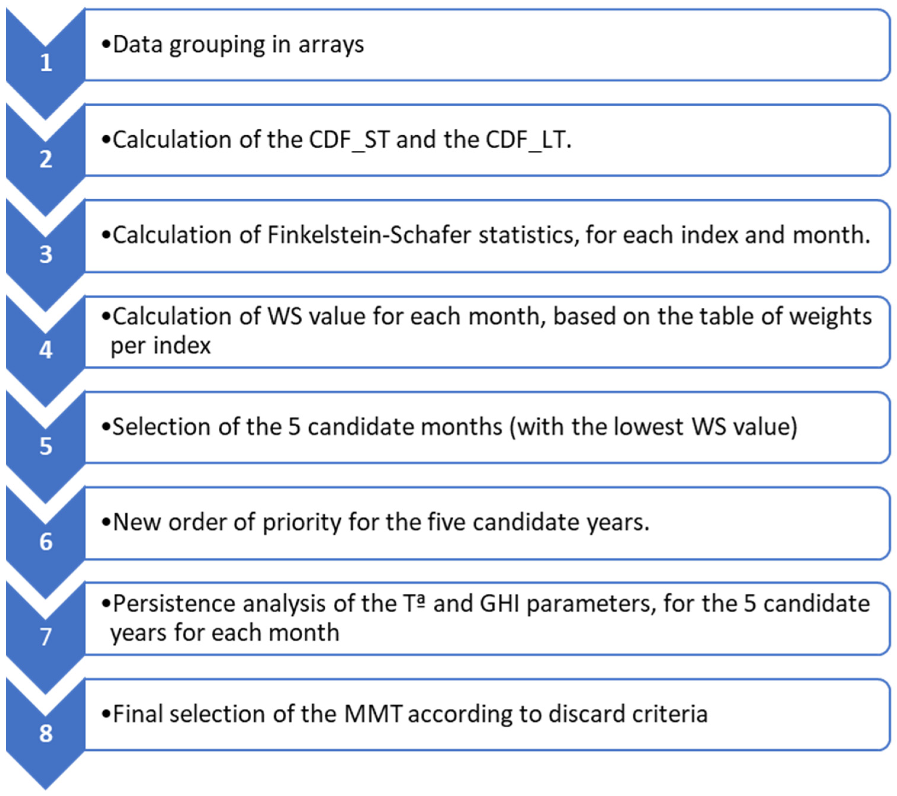
Once the average daily values of the nine climatic indices for the period 2008–2017 have been obtained, the 12 MMT can be determined (Figure 2).

In order to clarify the application of the procedure, the case of the MMT corresponding to the month of January at the Santiago EOAS weather station is shown as an explanatory example. In this case, for each of the indices, it is necessary to analyse the 10 months of January corresponding to the period from 2008 to 2017.

For each climatic index (i), it will be operated as follows:

• Data are grouped in a matrix, with as many rows as there are days in the month (January in this case) and as many columns as there are years in the period.
• The cumulative distribution functions will be calculated for the mean daily values for each month of January: CDF_{i, jany}, and the cumulative distribution function for the mean daily value corresponding to the entire period CDF_LT_{i, jan}. Applied to a parameter like f. ex the average daily temperature: DTm, the calculation of the CDF_{DTm, d, jan2008}, CDF _{DTm, d, jan2009}, …, CDF _{DTm, d, jan2017} and CDF_LT _{DTm, jan} is performed. The CDFs are calculated by applying Equation (3), and their value will be between 0 and 1.

$$CDF\left(i,d, m\right)=\{ \begin{array}{c}0, for x<x_1 ,\\ \frac{i}{n}, for x_{i } \le x \le x_{i+1}\\ 1, for x \ge x_n,\end{array} ,$$

(3)

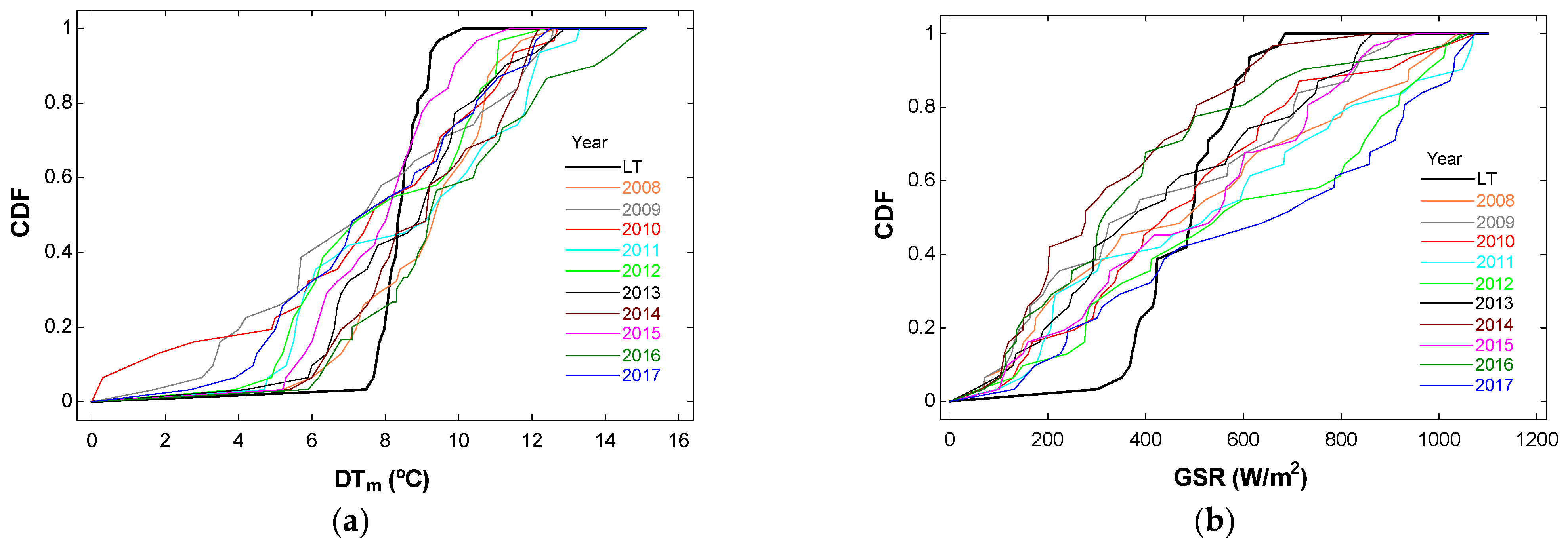
In Equation (3), i represents the ordinal of each day of the month and n represents the number of days in the month. Figure 3a shows the distribution functions obtained. Figure 3b shows, as a second example, the distribution functions obtained for the GHR index.

Taking into account the illustrations in Figure 3, it is verified that it is very difficult to identify at a glance which is the CDF_ST closest to the CDF_LT, therefore it is necessary to resort to a statistical procedure to quantify that degree of adjustment.

• Values of each CDF_i,d,m are sorted in ascending order and are compared month by month with the CDF_LT_i using the Finkelstein–Schaffer statistic [26]. The absolute maximum difference between the compared indices will be obtained. Equation (4) shows the example of calculating the FS statistic for the DTm index corresponding to the month of January 2008.

  Table 2. FS values for climatic indices obtained from the Santiago EOAS station (months of January, 2008–2017).

  Year	FSi
  	DTmax	DTmin	DTm	DPmax	DPmin	DPm	WVmax	WVm	GSR
  2008	0.2300	0.1904	0.2393	0.1894	0.2060	0.1436	0.2279	0.1863	0.2050
  2009	0.2518	0.2487	0.2414	0.2549	0.2445	0.2258	0.2268	0.1946	0.2216
  2010	0.1925	0.2102	0.2414	0.2050	0.2258	0.1967	0.1852	0.1915	0.1592
  2011	0.1956	0.2331	0.2477	0.2175	0.2144	0.2404	0.2206	0.1748	0.2081
  2012	0.1811	0.2549	0.2456	0.2300	0.2841	0.2404	0.4058	0.3548	0.2008
  2013	0.2227	0.1363	0.2216	0.2591	0.1519	0.1707	0.2331	0.2487	0.2019
  2014	0.1769	0.2248	0.1967	0.1946	0.2830	0.2092	0.2456	0.2268	0.2695
  2015	0.1988	0.1738	0.1717	0.2060	0.1467	0.1582	0.2945	0.3455	0.1904
  2016	0.2132	0.1604	0.2530	0.1865	0.1945	0.2518	0.2288	0.1710	0.2605
  2017	0.1727	0.2674	0.2268	0.1446	0.2560	0.2643	0.2945	0.3600	0.2164

  shows the set of calculated values of the FS statistic for the nine climatic indices and the ten months of January of the period.

  $$FS \left(DTm,jan2008\right)=\frac{1}{31}{\displaystyle {{\displaystyle \sum }}_{d=1}^{31}}\left|CD{F}_{DTm,d, jan2008}-CDF\_L{T}_{DTm,d, jan}\right|$$

  (4)

• Following the Sandia method, the comparison coefficient (WS) to be applied to each year of the analysis period must be obtained. Said value is obtained through Equation (5), where a relative weight is assigned to each climatic index according to the values in

  Table 3. Weight factor used in Sandia Laboratory method (w_i).

  DT			DP			WV		GSR
  Max	Min	Mean	Max	Min	Mean	Max	Mean
  1/24	1/24	2/24	1/24	1/24	2/24	2/24	2/24	12/24

  (1).

  $$WS={{\displaystyle \sum }}^{}{w}_i F{S}_i$$

  (5)

In Equation (5), w_i is the relative weight for index “i” and FS_i is the value of the FS statistic for index i

Table 4. Result of calculation of WS values for the month of January (Santiago EOAS).

Year	WS
2010	0.1822
2008	0.2029
2013	0.2059
2015	0.2063
2011	0.2135
2009	0.2265
2016	0.2371
2017	0.2387
2012	0.2439
2014	0.2446

presents a succession of years ordered according to the ascending value of WS calculated.

3.

In the next step, the 5 years with the least weight of the WS term will be selected. In this case, they are those corresponding to the years: 2010, 2008, 2013, 2015 and 2011. The worst value of WS is the one corresponding to the year 2014, with 0.2446, which indicates the largest deviation from the mean of the period.

The results of applying similar analyses to the twelve months of the period under study are presented below in

Table 5. Summary of the 5 years selected candidates for each of the MMT (Santiago EOAS station).

January	February	March	April	May	June	July	August	September	October	November	December
2010	2010	2011	2010	2010	2014	2014	2008	2011	2016	2010	2008
2008	2013	2014	2013	2009	2016	2011	2012	2010	2008	2013	2013
2013	2011	2017	2009	2016	2010	2015	2017	2008	2009	2011	2010
2015	2017	2008	2008	2012	2009	2017	2009	2013	2010	2017	2009
2011	2009	2015	2015	2014	2011	2008	2011	2012	2012	2009	2017

,

Table 6. Daily DTm temperature data for the month of January of the five selected years.

Day	5 Years with Lower Value of WS					Long Term Value (LT)
	2010	2008	2013	2015	2011	Mean LT
1	0.3	5.2	4.2	5.2	4.7	3.9
2	0.3	6.0	5.9	5.3	4.8	4.5
3	1.8	6.4	6.0	5.8	5.3	5.1
4	1.8	6.8	6.4	5.8	5.4	5.2
5	2.8	7.0	6.5	6.0	5.5	5.6
6	4.9	7.2	6.6	6.1	5.6	6.1
7	5.0	7.4	6.7	6.2	5.6	6.2
8	5.7	7.4	6.7	6.3	5.7	6.4
9	5.8	7.8	6.8	6.4	5.8	6.5
10	5.9	8.3	7.0	6.7	6.0	6.8	33rd percentile
11	6.7	8.4	7.5	7.1	6.1	7.2
12	6.9	8.9	7.8	7.3	6.6	7.5
13	7.4	9.2	7.8	7.7	7.0	7.8
14	7.4	9.2	8.6	7.8	8.5	8.3
15	7.7	9.4	8.9	8.0	9.1	8.6
16	7.7	9.4	9.0	8.2	9.3	8.7	Median
17	8.1	9.5	9.1	8.2	9.5	8.9
18	8.8	9.6	9.2	8.3	9.9	9.2
19	9.3	10.1	9.4	8.4	10.2	9.5
20	9.3	10.1	9.5	8.9	10.6	9.7
21	9.4	10.3	9.7	8.9	10.6	9.8	67th percentile
22	9.5	10.5	9.8	8.9	10.9	9.9
23	9.9	10.6	9.9	8.9	11.6	10.2
24	10.3	10.8	9.9	9.0	11.8	10.4
25	10.7	10.8	10.4	9.2	11.9	10.6
26	11.0	10.8	11.0	9.7	11.9	10.9
27	11.2	10.8	11.0	9.8	12.0	11.0
28	11.4	11.0	11.3	9.9	12.1	11.1
29	11.5	11.4	12.1	10.2	12.2	11.5
30	12.6	11.7	12.5	10.5	13.2	12.1
31	12.7	12.7	12.9	11.4	13.3	12.6
Mean	7.5	9.2	8.7	7.9	8.8	8.43
Median	7.7	9.4	9.0	8.2	9.3	8.72
33rd percentile	6.62	8.39	7.45	7.06	6.09	7.12
67th percentile	9.41	10.32	9.71	8.9	10.63	9.79
Dif 1	0.893	0.749	0.278	0.496	0.362
Dif 2	1.020	0.680	0.280	0.520	0.580

and

Table 7. Consistency analysis for the month of January 2013, with sorted values.

	Day	Sort	DTm	Day	Sort	GSR
	1	22	4.2	1	18	0.14
	2	21	5.9	2	17	0.26
	3	23	6	3	30	0.36
	4	6	6.4	4	25	0.38
	5	13	6.5	5	8	0.51
	6	7	6.6	6	23	0.53
	7	12	6.7	7	20	0.60
	8	20	6.7	8	31	0.68
	9	5	6.8	9	27	0.69
	10	14	7	10	9	0.77
	11	15	7.5	11	19	0.81	33rd per
	12	11	7.8	12	12	0.81
	13	19	7.8	13	15	0.82
	14	2	8.6	14	16	0.93
	15	24	8.9	15	29	0.99
	16	4	9	16	11	1.07
	17	28	9.1	17	28	1.22
	18	1	9.2	18	22	1.23
	19	26	9.4	19	10	1.31
	20	27	9.5	20	14	1.56
	21	25	9.7	21	26	1.59	67th per
	22	8	9.8	22	13	1.64
	23	3	9.9	23	1	1.69
	24	10	9.9	24	21	1.93
	25	17	10.4	25	2	2.00
	26	16	11	26	24	2.08
	27	29	11	27	5	2.09
	28	9	11.3	28	7	2.28
	29	18	12.1	29	3	2.30
	30	30	12.5	30	4	2.33
	31	31	12.9	31	6	2.40
		DTm			GSR
		Nº	Max long		Nº	Max Long
Below 33rd percentile		1	2		1	2
Above the 67th percentile		2	2
Nº invalids runs		0			0
Total runs per index		3			1
Total runs			3 + 1 = 4

.

4.

The next step to follow (Sandia method) is to establish a new order of priority for the five candidate years obtained.

Next, daily dry temperature data for the month of January for the 5 selected years are presented, as well as the daily average of the Long-Term (LT) period, all of them ordered from lowest to the highest temperature.

Terms AVERAGE and MEDIAN represent, respectively, the mean value of the daily mean temperatures of the dry bulb and the median of the same parameter in the analysed month of the five selected years and of the mean values of the total period.

Terms 33 and 67 percentiles, correspond to values for days located in those percentiles. As already indicated, days with temperatures below the 33rd percentile correspond to the coldest days of the month and those above the 67th percentile correspond to the hottest days of the month.

Term Dif1 expresses the difference between the average daily temperature of the month to be analysed and the average of the total period of each of the 5 selected years. Term Dif 2 corresponds to the differences of the medians.

Once the calculations of Dif1 and Dif2 have been made, the sum (Dif1 + Dif2) is performed per year and the years are ordered from the lowest to the highest value of the sum, giving rise to the order of preference of the following analysis. For the present example (January), they will be 1st—2013, 2nd—2015, 3rd—2011, 4th—2008 and 5th—2010.

5.

The process continues with the persistence analysis of the DTm and GHR indices, which consists of evaluating the frequency and length of the runs observed above and below the fixed long-term percentiles, following the order obtained in the previous step. For the DTm index, the frequency and length of the continuous run above the 67th percentile (consecutive hot days) and below the 33rd percentile (consecutive cold days) are determined. For the GSR index, the frequency and length of the run below the 33rd percentile (consecutive days of low radiation) are determined.

6.

For the final selection (Sandia method) and starting from the candidate years ordered by each month (Table 5), years will be excluded following the criteria:

• First: the years with the highest total number of consecutive strings
• Second: the year with the greatest number of strings of the greatest length
• Third: the years that do not present chains.

When two years meet the same conditions, the year located in the lower position of the table is eliminated.

The same procedure followed to select the best month of January has to be repeated to obtain the remaining 11 representative months corresponding to the Santiago Meteorological Station—EOAS, and this entire process must be reiterated, in order to obtain the corresponding Typical Meteorological Years to the remaining seven stations. The final result is shown in

Table 8. Typical meteorological years according to Sandia Laboratories methodology for the 8 stations, period 2008–2017.

Station Name	January	February	March	April	May	June	July	August	September	October	November	December
CIS Ferrol	2013	2014	2010	2008	2009	2014	2014	2017	2008	2015	2014	2014
Malpica	2013	2014	2008	2010	2012	2009	2014	2017	2017	2008	2014	2013
Santiago—EOAS	2013	2013	2015	2013	2014	2014	2014	2011	2010	2012	2017	2009
Campus Lugo	2011	2014	2008	2013	2014	2014	2017	2009	2014	2015	2014	2016
Pedro Murias	2015	2017	2014	2009	2012	2015	2014	2011	2012	2011	2010	2008
Estacións	2009	2010	2008	2008	2014	2014	2010	2014	2010	2016	2013	2016
Lourizan	2013	2015	2014	2013	2009	2009	2017	2011	2016	2016	2011	2012
Vigo-Campus	2013	2011	2015	2008	2014	2010	2008	2009	2010	2015	2016	2012

.

3. Generation of Climatic Files

3.1. Data Acquisition

Once the 12 TMM associated with a station have been selected, hourly data necessary to create the corresponding climatic file can be downloaded, but these must be concatenated to complete a Typical Meteorological Year (TMY). The procedure followed requires smoothing of the existing discontinuities in the interfaces between consecutive months. For this target, overlap will be made during the last 6 h of the outgoing month and the first 6 h of the incoming month, with the average values obtained from one and the other temperature profile.

In order to prepare the climatic file with Energy Plus™ (E+) format, historical databases of MeteoGalicia have been used. Hourly values of indices (temperature, relative humidity, atmospheric pressure, wind speed, wind direction and horizontal solar radiation) have been downloaded, however they do not provide values of the direct and diffuse components of radiation. To obtain these data, two alternatives were evaluated:

• Obtaining the diffuse component by one of the existing contrasted models [18,27,28,29,30,31], etc.
• Download solar radiation values from Satellite Databases (PVGIS, CAMS, SODA, Merra II, NSRBD, etc.).

In the present work, solar radiation values from 2005 to 2020 were downloaded from the latest version of SARAH 2.1 database [32], active since March 2022. Data from satellite images have many advantages: the data are complete, uninterrupted and objective [33].

3.2. Comparison of SARAH 2.1 Data vs. Ground Weather Stations

At this point, the validation procedure and comparative results between data provided by the two data sources are shown in order to verify the suitability of the SARAH.2.1 database [32] with respect to the values recorded by ground stations.

First of all, daily average values of global radiation were downloaded by each meteorological station, later a comparative analysis was carried out to verify the differences between both data sources.

As an application example,

Table 9. Comparative results for GHR (Santiago EOAS station, 2008–2017).

	MeteoGalicia	PVGIS-SARAH 2.1
Average	3.631	3.891
Típical error	0.159	0.169
Median	3.721	4.047
Standard deviation	1.747	1.856
Sample variance	3.052	3.446
Curtosis	−1.368	−1.423
Skewness coefficient	0.024	0.062
Range	6.047	6.225
Mínimum	0.933	1.137
Máximum	6.980	7.362
Addition	435.7	466.9
Number	120	120
Confidence level (95.0%)	0.316	0.336
Correlation coef. R² (daily values)		0.985

presents the results for the Santiago EOAS station. A high degree of correlation is observed between data from both sources.

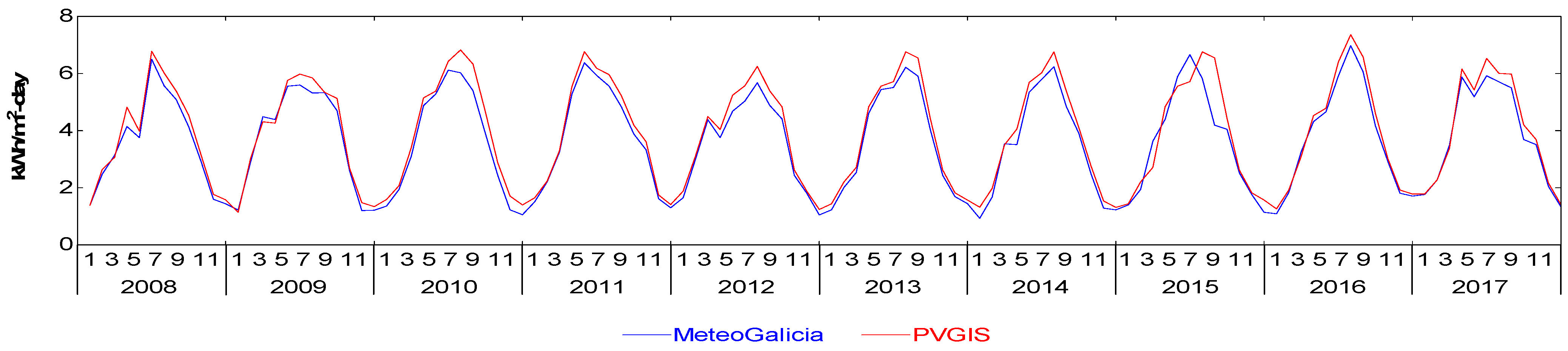
Figure 4 and Figure 5 graphically show the concordance and trend similarity of Global Horizontal Radiation data obtained from both sources.

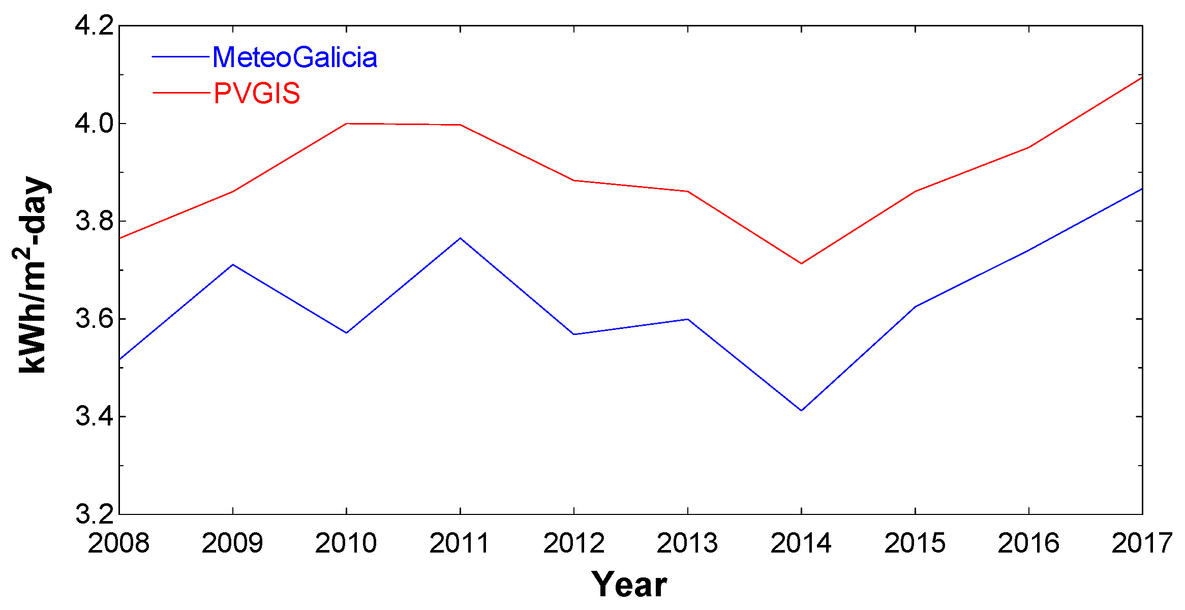
As can be seen in

Table 10. Summary comparative study for the 8 stations (period 2008–2017).

Station	Cor. Coef. R²	GHI Mean			St. Dev.		Range		Minimum Value		Maximum Value		Y. Sum
		MeteoG	SARAH	dif (%)	MeteoG	SARAH	MeteoG	SARAH	MeteoG	SARAH	MeteoG	SARAH	MeteoG	SARAH
Ferrol cis	0.9879	3.618	3.726	3.0%	1.754	1.780	5.810	5.858	0.918	1.070	6.728	6.928	434.117	447.131
Malpica	0.9880	3.765	3.712	−1.4%	1.793	1.704	5.932	5.362	1.108	1.229	7.040	6.591	451.856	445.443
Santiago Eoas	0.9852	3.631	3.891	7.2%	1.747	1.856	6.047	6.225	0.933	1.137	6.980	7.362	435.660	466.892
Lugo campus	0.9859	3.562	3.873	8.7%	1.766	1.905	6.045	6.267	0.972	1.201	7.017	7.468	427.492	464.781
Ribadeo	0.9805	3.227	3.413	5.8%	1.464	1.420	4.539	4.575	1.001	1.162	5.540	5.737	387.255	409.575
Orense	0.9922	3.838	4.048	5.5%	2.001	1.974	6.356	6.292	0.997	1.216	7.354	7.508	460.502	485.803
Lourizan	0.9903	3.806	4.098	7.7%	1.840	1.970	6.447	6.766	0.996	1.156	7.443	7.922	452.865	487.614
Vigo campus	0.9875	4.098	4.189	2.2%	1.999	1.993	7.708	6.750	0.604	1.206	8.312	7.956	487.693	498.518

, in general, global values recorded in SARAH2.1 are higher than those recorded by MeteoGalicia, which may be due to different reasons. However, these variations are within the allowable ranges [34].

4. Results and Discussion

Climate files have been generated for 8 locations in Galicia (NE of the Iberian Peninsula) following the SANDIA method. For each location, two other files have been created, called: LT and WY in order to analyse the accuracy of the files generated with the Sandia method and to obtain a comparison reference.

• LT: files generated with average values of climatic indices between 1 January 2008 and 31 December 2017.
• WY: files generated taking as TMM those with the highest values of WS. In the case of Santiago EOAS, the year 2011 is used (Table 4).

The statistics used for the analysis are the following:

• Mean BiasError (MBE). Equation (6): mean of the algebraic sum of the estimated values and the corresponding reference values.

  $$MBE=\frac{1}{N}{\displaystyle {{\displaystyle \sum }}_{i=1}^N}\left(Ci-Mi\right)$$

  (6)
• Mean Absolute Error (MAE). Equation (7): sum of the absolute value of the deviations, divide by the number of values in the series.

  $$MAE=\frac{1}{N}{\displaystyle {{\displaystyle \sum }}_{i=1}^N}\left|Ci-Mi\right|$$

  (7)
• Root MeanSquare Error (RMSE). Equation (8): The root means square error (RMSE) is used to measure the accuracy of the model. The difference (error) occurs due to randomness or because the model does not consider information that could produce a more accurate estimate. Since the difference (Ci-Mi) is squared, large errors will have a greater impact.

  $$RMSE=\sqrt{\frac{1}{N}{\displaystyle {{\displaystyle \sum }}_{i=1}^N}{\left(Ci-Mi\right)}^2}$$

  (8)

In Equations (6)–(8), Ci is the reference value according to the model used, Mi: is the value to compare with the reference value and N is the number of values in the series.

• MBE: Mean Bias Errors of SANDIA and WY, respectively with respect to LT
• MAE: Mean Absolute Errors of SANDIA and WY, respectively with respect to LT
• RMSE: Root Mean Square Error of SANDIA and WY, respectively with respect to LT.

Table 11. Summary comparative study for the Santiago EOAS station (period 2008–2017).

	MBE		MAE		RMS
	SANDIA	WY	SANDIA	WY	SANDIA	WY
DT (°C)	0.09	−0.96	0.16	1.36	0.21	1.51
RH (%)	−0.58	5.08	1.08	6.08	1.19	7.23
GSR (Wh/m²)	118.42	−392.67	209.92	712.00	298.57	848.00
WV (m/s)	−0.04	−0.05	0.09	0.30	0.15	0.40

shows as an example the Errors for the parameters: Dry Temperature, Relative Humidity, Horizontal Global Solar Radiation and Wind Speed, corresponding to the Santiago EOAS station.

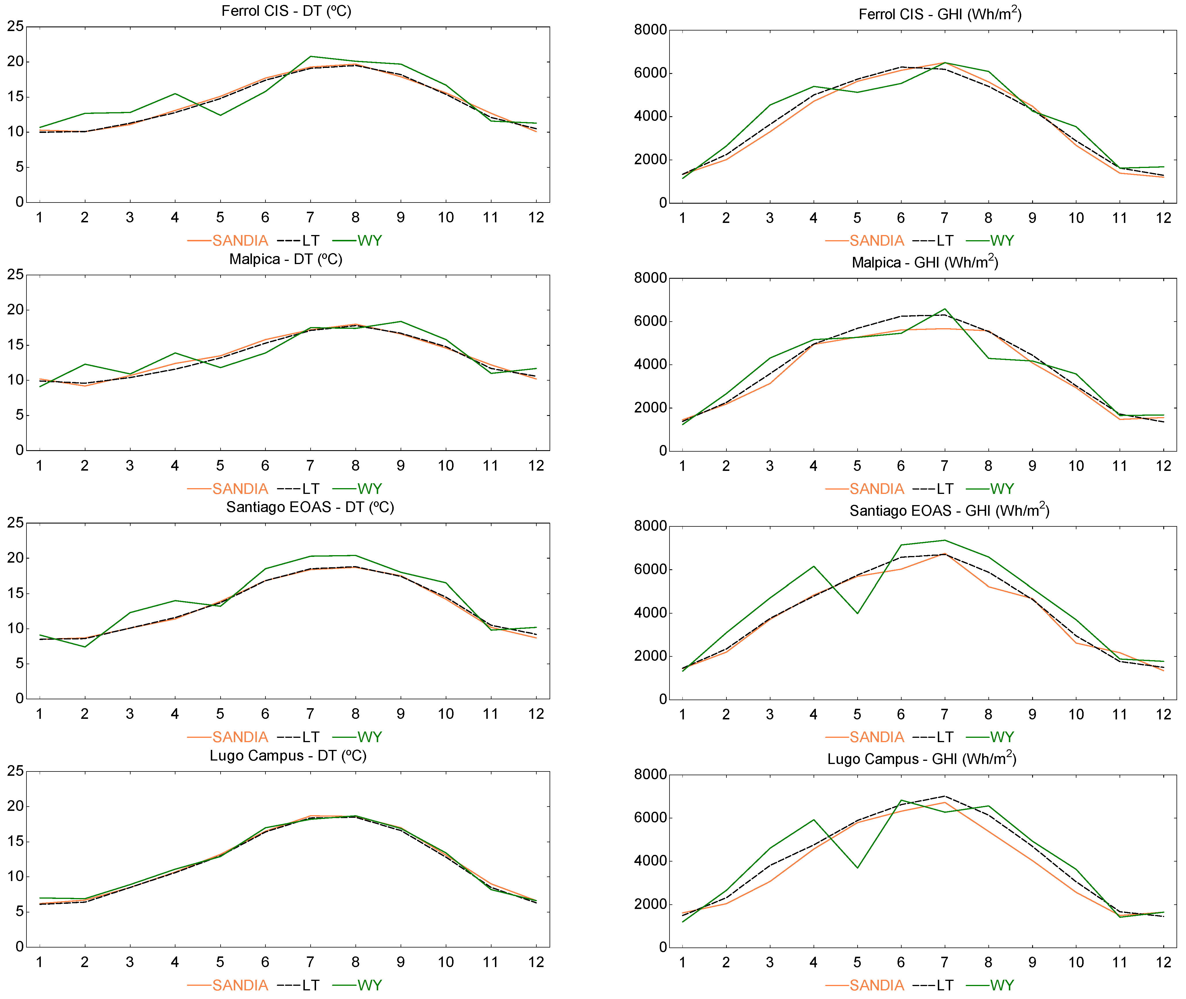
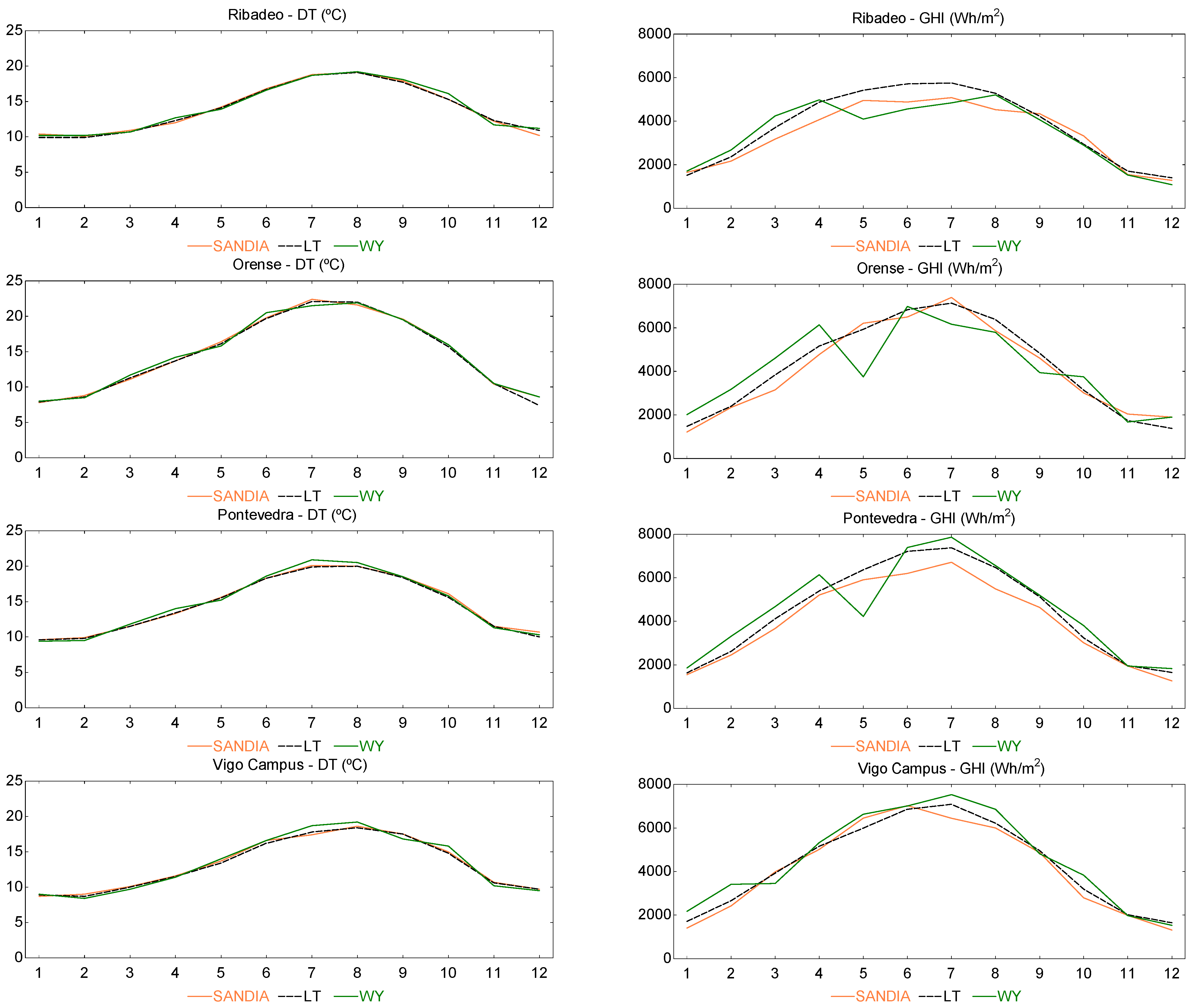
As can be seen in Table 11 and Figure 6, errors due to the Sandia method in the four parameters are, in all cases, significantly lower than those caused by taking the WY. This indicates that files generated with the Sandia method are closer to those generated with the average values of the period (LT). Error Statistics for the 8 stations are shown in

Table A1. DT error statistics for the 8 stations.

Temperature—DT (°C)
Station	MBE1	MBE2	MAE1	MAE2	RMSE1	RMSE2
Ferrol cis	0.13	−0.62	0.28	1.57	0.31	1.73
Malpica	−0.16	−0.42	0.34	1.20	0.39	1.39
Santiago eoas	0.09	−0.96	0.16	1.36	0.21	1.51
Lugo campus	−0.23	−0.31	0.23	0.41	0.27	0.46
Pedro murias	−0.02	−0.14	0.21	0.29	0.29	0.37
Estacions	−0.14	−0.18	0.28	0.37	0.41	0.50
Lourizan	−0.13	−0.19	0.15	0.36	0.26	0.43
Vigo campus	−0.09	−0.15	0.19	0.48	0.23	0.57

,

Table A2. RH error statistics for the 8 stations.

Relative Humidity—RH (%)
Station	MBE1	MBE2	MAE1	MAE2	RMSE1	RMSE2
Ferrol cis	0.00	0.33	2.67	3.00	3.16	3.65
Malpica	1.67	2.92	1.83	3.25	2.58	4.13
Santiago eoas	−0.58	5.08	1.08	6.08	1.19	7.23
Lugo campus	0.42	0.25	0.75	0.92	0.87	1.12
Pedro murias	0.17	−0.67	1.00	0.83	1.08	1.15
Estacions	−0.58	0.17	0.92	1.50	1.26	1.83
Lourizan	−0.50	1.00	1.50	1.17	1.83	1.63
Vigo campus	−0.17	2.08	1.50	3.25	1.91	3.57

,

Table A3. GHR error statistics for the 8 stations.

Global Horizontal Radiation—GHR (W/m2/Day)
Station	MBE1	MBE2	MAE1	MAE2	RMSE1	RMSE2
Ferrol cis	−81.7	−256.3	193.8	512.3	215.5	603.4
Malpica	−216.4	−182.3	269.4	457.8	345.8	625.1
Santiago eoas	118.4	−392.7	209.9	712.0	298.6	848.0
Lugo campus	305.3	−37.8	358.8	620.9	426.5	832.3
Pedro murias	326.4	251.4	431.4	442.6	510.9	613.6
Estacions	101.8	30.6	329.5	752.8	370.3	910.3
Lourizan	426.4	−135.7	426.4	496.5	528.7	745.0
Vigo campus	144.0	−258.5	257.5	388.2	310.5	456.7

and

Table A4. WV error statistics for the 8 stations.

Wind Velocity—WV (m/s)
Station	MBE1	MBE2	MAE1	MAE2	RMSE1	RMSE2
Ferrol cis	3.29	3.15	3.29	3.28	3.79	3.79
Malpica	0.88	0.87	1.11	1.30	1.46	2.09
Santiago eoas	−0.04	−0.05	0.09	0.30	0.15	0.40
Lugo campus	−0.13	−0.10	0.14	0.12	0.21	0.15
Pedro murias	−0.17	−0.03	0.17	0.14	0.20	0.18
Estacions	−0.10	−0.05	0.12	0.07	0.14	0.09
Lourizan	−0.08	−0.03	0.09	0.04	0.13	0.06
Vigo campus	−0.38	−0.18	0.39	0.29	0.56	0.36

.

As can be seen in Figure 6 and corroborated in the statistical analysis, the monthly evolution of the parameters obtained by the SANDIA method are very close to LT, thus confirming that the Sandia method is suitable for the selection of the MMT in order to prepare climate files for the region studied.

Looking at

Table 12. Comparative table of annual mean values for the 8 stations (period 2008–2017).

Station	DTm	HR	WV	GHI	Climatic Zone
CIS Ferrol	14.39	80.92	6.04	3.750.17	C1
Malpica	13.38	86.50	6.83	3.659.67	C1
Lourizan	14.59	81.75	1.23	4003.42	C1
Estacións	14.68	73.17	1.32	4085.33	C3
Santiago—EOAS	13.09	82.67	2.38	3891.58	D1
Campus Lugo	12.07	79.67	1.62	3769.75	D1
Pedro Murias	13.99	79.33	2.75	3415.92	D1
Vigo-Campus	13.22	75.08	2.72	4140.58	D1

, it can be observed the lack of precision produced, for example: including Campus Lugo and Pedro Murias in the same climatic zone: the average annual temperature difference is 1.92 °C (13.7%). Or distinguishing the climates of Lourizan (Pontevedra) and Estacions (Orense) when their annual climatic averages (DTm, WV and GHI) are very similar.

5. Conclusions

In the present work, a set of eight climatic files has been created, corresponding to as many meteorological stations, representative of the wide climatic diversity existing in Galicia. The Sandia method was used to obtain the respective Typical Meteorological Years (TMY), over a data range of 10 years. This procedure is explained step by step and a series of intermediate results are included in such a way that it is possible to monitor it by third parties.

It is observed that with the eight files generated, new differentiated climates are detected, which will affect the improvement of the precision of the energy simulations of buildings that are going to be carried out.

A widely tested and proven methodology has been used: the Sandia Laboratories method. As specific improvements:

• A practical case has been applied by means of an example so that other researchers can easily understand and apply the procedure.
• In this particular case, the dew temperature data have been obtained by means of psychrometric transformations from other available variables.
• Data from ground stations have been combined with data from satellite records in order to generate the final climate files.

The data series from satellite sources have been validated against mean values from ground stations by means of typical statistics. Additional controls have been applied to detect deviations and check the degree of adjustment to the Long-Term reference.

Regarding other published material, the novelty is that climatic files have been generated using in any case data from real measurements. For this, it has been necessary to resort to records from satellite databases and, after validation, combine them with data from ground stations.

The conclusions of this work must be considered by the administrations involved when drafting new versions of the Spanish legal texts that regulate energy efficiency requirements.

The topic is certainly relevant: it is pointing to a lack of harmonization in the application of construction requirements in buildings as well as a deviation in the results of the calculations of energy balance and estimation of CO₂ emissions into the atmosphere.

Obtaining a new complete set of climatic files capable of collecting the microclimatic diversity of Galicia will be very useful for the homogenization of the energy simulation processes of buildings and energy installations in the region and, consequently, for the harmonization of construction requirements for buildings subject to similar thermal demands. The policy on energy efficiency is defined by the central government, but this reality should be considered when drafting new versions of the legal texts that regulate energy efficiency requirements.

The final conclusions are in line with the results obtained, which have evidenced the initial expectation of the lack of resolution of the currently existing climate files for energy simulation.

The algorithm created to automate the entire process followed has been implemented in spreadsheets, so it would be immediate to process datasets corresponding to new locations or different ranges of years.

References

- Ministerio de Fomento- Gobierno de España. Código Técnico de la Edificación Real Decreto 314/2006; Ministerio de Fomento- Gobierno de España: Madrid, Spain, 2006. [Google Scholar]
- U.S. Department of Energy. EnergyPlus™ Version 8.8.0 Documentation Auxiliary Programs; U.S. Department of Energy: Lemont, IL, USA, 2017.
- Hall, I.; Prairie, R.; Anderson, H.; Boes, E. Generation of Typical Metereological Years for 26 SOLMET Stations; SAND78-1601; Sandia Laboratories: Albuquerque, NM, USA, 1978. [Google Scholar]
- Crow, L.W. Development of Hourly Data for Weather Year for Energy Calculations (WYEC). ASHRAE J. 1981, 23, 37–40. [Google Scholar]
- Klein, S.A.; Beckman, W.A.; Duffie, J.A. A design procedure for solar heating systems. Sol. Energy 1976, 18, 113–127. [Google Scholar] [CrossRef]
- ASHRAE. International Weather for Energy Calculations 2.0; American Society of Heating, Refrigerating and Air-Conditioning Engineers: Atlanta, GA, USA, 2012. [Google Scholar]
- Lund, H. The Design Reference Year; report N° 274; Thermal Insulation Laboratory, Technical University of Denmark: Lyngby, Denmark, 1995. [Google Scholar]
- Pissimanis, D.; Karras, G.; Notaridu, V.; Garga, K. The generation of a typical metereological year for the city of Athens. Sol. Energy 1988, 40, 405–411. [Google Scholar] [CrossRef]
- NORMA UNE ISO 15927-4; Datos Horarios Para la Evaluación de la Energia Anual Utilizada en Calefacción y Refrigeración. AENOR—Asociación Española de Normativa y Certificación: Madrid, Spain, 2011.
- Bre, F.; Fachinotti, V. Generation of typical metereological years for the Argentine Litoral Region. Energy Build. 2016, 129, 432–444. [Google Scholar] [CrossRef]
- Huld, T.; Paietta, E.; Zangheri, P.; Pinedo Pascua, I. Assembling Typical Meteorological Year Data Sets for Building Energy Performance Using Reanalysis and Satellite-Based Data. Atmosphere 2018, 9, 53. [Google Scholar] [CrossRef]
- Bilbao, J.; Miguel, A.; Franco, J.A.; Ayuso, A. Test Reference Year Generation and Evaluation Methods in the Continental Mediterranean Area. J. Appl. Meteorol. 2004, 43, 390–400. [Google Scholar] [CrossRef]
- Casa, F.; Echeverría, E.; Celis, F. Climate zoning for its application to bioclimatic design. Application in Galicia (Spain). Informes de la Construcción 2017, 69, 547. [Google Scholar]
- Martínez, A.; Castillo, F.; Pérez, A.; Valcárcel, M.; Blanco, R. Atlas Climático de Galicia; Xunta de Galicia: Santiago de Compostela, Spain, 1999. [Google Scholar]
- Pettazzi, A.; Salsón, S. Atlas de radiación solar de Galicia. XUNTA DE GALICIA Conselleria de Medio Ambiente, Territorio e Infraestructura (MeteoGalicia, Área de Observación e Climatoloxía), Santiago de Compostela. 2011. Available online: https://www.meteogalicia.gal (accessed on 1 September 2022).
- Marion, W.; Urban, K. User´s Manual for TMY2s—Typical Metereological Years; National Renewable Energy Laboratory—U.S. Department of Energy: Golden, CO, USA, 1995.
- Sawaqued, N.; Zurigat, Y.; Al-Hinai, H. A step-by-step application of Sandia method in developing typical metereological years for different locations in Oman. Int. J. Energy Res. 2005, 29, 723–737. [Google Scholar] [CrossRef]
- Couce, A.; López, I.; Lamas, I.; Rodríguez, J. Creation of a Typical meteorological Year in Spain. Step by step application of the method based on UNE-EN ISO-15927-4:2011. DYNA, 2022; in press. [Google Scholar]
- QGIS.org. QGIS Geographic Information System. QGIS Association, 2022. Available online: http://www.qgis.org (accessed on 1 September 2022).
- Antoine, C. Tensions des vapeurs; nouvelle relation entre les tensions et les températures. de Comptes Rendus des Séances de L’académie des Sci. 1888, 107, 681–684, 778–780, 836–837. [Google Scholar]
- Tetens, O. Über einige meteorologische Begriffe. Z. Geophys. 1930, 6, 297–309. [Google Scholar]
- Buck, A. New equations for computing vapor pressure and enhancement factor. J. Appl. Meteorol. 1981, 20, 1527–1532. [Google Scholar] [CrossRef]
- Magnus, G. Versuche über die Spannkräfte des Wasserdampfs. Ann. Phys. Chem. 1844, 61, 225–247. [Google Scholar] [CrossRef]
- Ministerio de Fomento Secretaría de Estado de Infraestructuras, Transporte y Vivienda Dirección General de Arquitectura, Vivienda y Suelo, Documento descriptivo climas de referencia, Madrid. 2017. Available online: http://www.codigotecnico.org (accessed on 1 September 2022).
- R Core Team. R: A Language and Environment for Statistical Computing; R Foundation for Statistical Computing: Vienna, Austria, 2020; Available online: https://www.R-project.org/ (accessed on 1 September 2022).
- Finkelstein, J.; Schafer, R. Improved Goodness-of-Fit Tests. Biom. Trust 1971, 58, 641–645. [Google Scholar] [CrossRef]
- Liu, B.; Jordan, C. The interrelationship and characteristic distribution of direct, diffuse and total solar radiation. Sol. Energy 1960, 4, 1–19. [Google Scholar] [CrossRef]
- Orgill, J.; Hollands, K. Correlation equation for hourly diffuse. Sol. Energy 1977, 19, 357–359. [Google Scholar] [CrossRef]
- Reindl, D.; Beckman, W.; Duffie, J. Diffuse fraction correlations. Sol. Energy 1990, 45, 1–7. [Google Scholar] [CrossRef]
- Perez, R.; Ineichen, P.; Seals, R.; Michalsky, J.; Stewart, R. Modeling daylight availability and irradiance components from direct and global irradiance. Sol. Energy 1990, 44, 271–289. [Google Scholar] [CrossRef]
- Maxwell, E. A Quasi-physical Model for Converting Hourly Global Horizontal to Direct Normal Insolation. Sol. Energy Res. Inst. 1987, 1, 1–55. [Google Scholar]
- PVGIS, PVGIS VER 5.2. Available online: https://re.jrc.ec.europa.eu/pvg_tools/en/ (accessed on 1 September 2022).
- Huang, Y. Using Satellite-Derived Solar Radiation to Create Weather Files of Unprecedented Accuracy and Reliability. In Proceedings of the 16th IBPSA Conference, Rome, Italy, 2–4 September 2019. [Google Scholar]
- Pfeifroth, U.; Trentmann, J.; Kothe, S. Meteosat Solar Surface Radiation and Effective Cloud Albedo Climate Data Record, SARAH-2.1; Validation Report; Satellite Application Facility on Climate Monitoring (CM SAF): Strahlenbergerstr, Germany, 2019. [Google Scholar] [CrossRef]
Figure 1.
Selected weather stations and population areas of influence [
19].
Figure 2.
Flowchart of the selection process for the 12 TMM according to Sandia method.
Figure 3.
Santiago EOAS Station, the month of January (R Statistics [
25]): (
a) Representation of
CDF functions for the Daily Mean Temperature index; (
b) Representation of
CDF functions for the Daily Mean Horizontal Global Radiation index.
Figure 4.
Evolution of the monthly mean GHR index: PVGIS vs. MeteoGalicia (Santiago EOAS, 2008–2017).
Figure 5.
Evolution of the annual mean GHR index: PVGIS vs. MeteoGalicia (Santiago EOAS, 2008–2017).
Figure 6.
Comparison of the monthly evolution of dry bulb temperature (DT) and solar irradiation (GHI) for the 8 stations.