1. Introduction
Resilience of the product, labor, and financial markets are typically considered as robust buffers against disruptive shocks to the macroeconomy. Recently,
Brunnermeier (
2021) has referred to the concept of resilience to explain the stability of the macroeconomy during normal times. There are, however, also factors such as resiliency destroyers that can undermine resilience and can lead to disruptive dynamics. In
Semmler et al. (
2023), the theory of resilience is evaluated from the perspective of complex system dynamics across various time scales. Various model versions examine the concept of resilience as local resilience (corridor stability) and global resilience (global stability). The analysis reveals the existence of endogenous economic resilience, sudden resilience breakers, loss of resilience, disruptive contractions, or persistent cycles. However, achieving resilience involves extensive monetary, financial, and fiscal policies.
Previous studies on complex features and shock responses suggest that small shocks typically have temporary effects, while larger shocks can give rise to various phenomena, including significant disruptions. These disruptions can be mitigated through policy interventions, which aim to stabilize the system but do not necessarily restore steady-state growth. Instead, they may result in the emergence of further cycles. This behavior is often captured using the concept of Hopf bifurcation, which describes a locally unstable dynamic that can exhibit globally cyclical dynamics under the influence of policies. In this paper, we take a step further by outlining different variants of a dynamic model. Using U.S. time-series data, we estimate the dynamics of the financial–real interaction, specifically focusing on the liquidity dynamics within the financial sector.
We estimate econometrically the model through a Smooth Transition Regression
method. The econometrically estimated dynamic model shows the existence of such complex system dynamics, which can be vulnerable to loss of resilience and contractions. In this empirical paper, we explore some features first addressed by
Semmler and Koçkesen (
2017). In our empirics, we first need to transform our analytically studied continuous-time form into an estimable discrete-time form employing the discrete-time Smooth Transition Regression
methodology. Our estimation procedure is applied to the U.S. time-series data for a certain time period. Hereby, we can show the existence of cyclical solution paths, if supported by sufficient policies, and demonstrate that the empirics of financial–real forces can indeed exhibit multiple features and even robustness of large shocks when policy interventions are effective.
Technically, the essential nonlinearities and regime changes can generate a locally stable or unstable equilibrium responding to small shocks. Additionally, it can exhibit global resilience, characterized by persistent (limit) cycles as predicted by the Hopf bifurcation type dynamics, which assumes unstable dynamics close to the equilibrium but stabilizing forces activated further out. The econometrically estimated model reveals the existence of local non-resilience and global resilience. For the locally unstable but globally bounded fluctuations—global resilience—we can detect asymmetric responses to shocks. Furthermore, certain dynamics within the system can lead to disruption and traps, as we highlight in our analysis.
The remainder of the paper is organized as follows. In
Section 2, we will sketch some nonlinear model variants of the liquidity–macro link to explain the above scenarios.
Section 3 presents simulations featuring some of the above-mentioned complex outcomes for small and large shocks. In
Section 4, we estimate econometrically the model through the Smooth Transition Regression
method for U.S. time-series data.
Section 5 provides some conclusions. In
Appendix A, some technical details are presented.
2. Sketch of Nonlinear Model Variants and Simulations
We start with a sketch of the basic dynamic model augmented by two perturbation terms that are decisive for the dynamics. The basic part of our model is consistent with a monetary growth model with an explicit
schedule. We will provide a sketch of the dynamic models and conduct a series of simulations to demonstrate the possible dynamics of the model. Using a Lyapunov function, we can assess whether the dynamic system tends to stay near its equilibrium point or drift away from it.
1 2.1. Analytical Model Variants
The basis of our presentation here is a model that is grounded in an version for a growing real economy that links output to liquidity and credit flows. It assumes that financial flows to economic agents (to households and firms) are related to the balance sheets of the economic agents. We assume that when the agents’ balance sheets deteriorate (improve), creditworthiness and credit flows deteriorate (improve). Based on the literature cited above, credit conditions, specifically creditworthiness, and consequently the spending behavior of economic agents, are influenced by both liquidity on the financial side and the dynamics of output and real income on the real side.
We use the broad definition of liquidity as a measure of liquidity: cash, deposits, credit and credit lines from banks, and short-term treasury bonds. We usually observe that at high levels of economic expansion, liquidity rises, default risk falls, and asset prices and creditworthiness rise. The reverse may be assumed to happen during a low level of economic activity. As liquidity shrinks, default risk rises, asset prices fall, and creditworthiness and credit provisions fall. Concerning spending, we may thus assume that spending accelerates (decelerates) when output and liquidity rise above (fall below) some threshold level. The main features of a dynamic model of liquidity, credit, and output in a growing economy can cause regime changes triggered by state-dependent reactions. These reactions can be expressed in a deterministic form as follows.
We presume that economic agents respond to both financial variables (balance sheet variables) and real variables. In the generic form, the financial variables are and real variables are , with L denoting liquidity, a balance sheet variable, Y, output (or real income), a real variable, and K the capital stock, while and represent the growth rates of both ratios, respectively. When we undertake the empirical estimate with data on firms, we interpret real income, Y, as a firms’ income and as a firms’ income relative to capital stock. Thus, denotes the rate of return on real capital.
A model of the type as shown in Equation (
1) can be derived from an aggregate model, assuming that the firms’ income is linear in aggregate income.
In simple terms, model (
1) establishes a connection between variations in income and liquidity, linking them with fluctuations in liquidity and income. The term
denotes the liquidity that is used for growth and new transactions and is thus used in the second equation as the term
for households and firms. Parameter
represents the natural dissipation of capital value, for example due to depreciation. On the other hand, in the absence of a new injection of liquidity, the income growth rate is firmly negative, thus pushing the income toward zero if no new liquidity is provided. There is a cross-dual interdependence since the growth rate of each variable depends on the other state variable. Note that, due to this last property of model (
1), the positive quadrant
,
is invariant, which means that if we start with positive liquidity and income, they will remain positive forever.
Our actual model can be thought of as being composed of two parts. First, a basic part of the model that exhibits no thresholds and regime changes can be expressed linearly as system (
1). Our basic dynamic equations can then be defined as follows, and are easily shown to be constant along trajectories of the model of Equation (
1) where no other terms appear so far.
2 Usually, when such a model is solved, one can observe trajectories that oscillate around a common center point with the same cycle length. The cyclical relationship it exhibits is similar to a predator–prey system. We can then introduce some perturbation terms and call this the basis for system (I).
3Here, the coefficients
,
,
,
,
, and
are positive. In model (
2),
represents the natural liquidity growth, for example, through the central bank’s growth rate of liquidity (money) supply. The terms
and
prevent the liquidity and income from growing without bounds. The additional terms will then create some reversions to the steady state.
The model of Equation (
2) is a nonlinear system of differential equations of Lotka–Volterra type, which originated in the 1920s in the mathematical studies of interacting species, with
and
as perturbation terms. However, this system of Equation (
2) has three equilibria (
,
,
, and
. The first two are saddle points, and the last one is an attraction point. Except for those that start on one of the axes, all of the trajectories converge to the unique attracting point
,
. The dynamics of the model of Equation (
2) will be simulated below by choosing economically realistic parameters. For a more detailed discussion of the subsequent subsections, including the perturbation term, corridor stability cycles, and a limit cycle outside an asymptotically stable region, please refer to
Semmler et al. (
2023).
2.2. System I
Regarding the system described in Equation (
2), it is important to consider the potential dynamics influenced by an additional perturbation term referred to as
. This term represents a weak perturbation that can be activated with varying degrees of strength. The function
represents the idea that, during business contractions, there is a reduced willingness among lenders, such as depositors or banks, to deposit cash or a tendency to decrease deposits. Additionally, banks may lower credit lines offered to firms and households, all of which are contingent upon the condition of the banks, firms, or households. In addition, if agents anticipate insolvencies or bankruptcies, withdrawing liquidity becomes eminent as a means to safeguard financial assets for worse times. However, the dissipation of liquidity will entail a decline in liquidity flow to households and firms, leading to lower capital outlay and investment, possibly setting in motion complicated dynamics.
4Formally, concerning the function
, we assume that if the rate of return for firms falls below a certain rate of return,
with
, and/or if simultaneously liquidity drops below a certain ratio,
with
, there will be a strong dissipation of liquidity. This, in turn, will have a corresponding impact on the capital outlay and investment of firms and the spending of households. Consequently, we replace model Equation (
2) with the following system of differential equations.
The term
in Equation (
3) serves as a control term in our dynamic system. It captures the response of banks and firms when the liquidity ratio falls below the threshold
and when the rate of return drops below the threshold
.
5 Hereby, the impact on contractions becomes stronger. We shall assume that
in Equation (
3) is a smooth function satisfying the following conditions:
For our simulation, we chose the following:
In addition, we make the assumption that
and
. Subsequently, we label the nonlinear differential Equation (
3) as system (I). Equation (
3) can also be employed to explain system (II) described below, although in system (II) the effect of
remains large. The coefficient
v refers to the reaction coefficient or perturbation term that, given different values, helps understand any type of convergence.
The proposition that system (I), represented by model of Equation (
2), remains stable in the vicinity of the equilibrium holds true even when
is activated. This is because the Jacobian matrix at
yields the same local dynamic outcomes for Equation (
3) as it does for Equation (
2). Whereas the term
pushes the trajectories toward the axes, as soon as
and
decline below
and
, the terms
and
generate attracting forces, keeping the trajectories in a compact set. So for a small
and small shocks, we may still have convergence toward the steady state
, as in Equation (
2).
2.3. System II
Therefore, system (I) exhibits two distinct scenarios. In the case of a small reaction coefficient,
v, the trajectories still converge towards the equilibrium for small shocks. However, this convergence does not hold when
v becomes larger. In the context of system (I), we can assume that
v is active but remains sufficiently small. In contrast, we designate system (II) as the case when
v is significantly larger and is triggered by larger shocks. An effective approach to demonstrate the potential scenarios is through a simulation study, as depicted in the upcoming simulations in
Section 3.
In summary, system (II) represents a scenario where the value of
v is sufficiently large.
6 To construct our simulation, we also choose
, but this time with high values of
v. Similarly, we use this nonlinear differential Equation (
3) to represent system (II). Below, we present the results for unstable dynamics, with
, allowing the reaction parameter
v to become even larger. The immediate effect is that there will be strong disruptions since the trajectories approach zero, and all values go down to zero.
2.4. System III
However, there remains a possibility of certain attractive forces even in the case of large shocks. This occurs in the presence of a limit cycle, which can be observed when , as illustrated below. A similar occurrence is observed when . In this case, one cycle is repelling and the other is attracting. The system could be stable for trajectories starting close to the equilibrium. Only a stronger shock, i.e., initial conditions far enough from the equilibrium, will generate persistent fluctuations and limit cycles. Thus, the system could exhibit corridor stability, then some regions of instability, but then again, for large shocks, some global stability, i.e., global resilience.
Regardless, certain parameter values of
v lead to the presence of a single limit cycle that exhibits both inward and outward attraction. This existence can be demonstrated using the Hopf bifurcation theory, which refers to the transition from a stable equilibrium (where it remains unchanged over time) to a situation where it exhibits periodic or oscillatory behavior. This type of persistent cycle will be studied below in Dynamics III and also empirically in
Section 4.
For stronger shocks, i.e., for farther departure from the equilibrium values of and , system (III) may locally become unstable. However, it remains globally bounded as it converges towards a limit cycle, even in the case of large shocks. Thus, for initial conditions farthest away from the equilibrium, the limit cycle is approached from the outside.
3. Numerical Simulations
Next, we will simulate the above three types of dynamics. In general, the subsequent simulation study uses the following parameters: , and . The economically relevant equilibrium is .
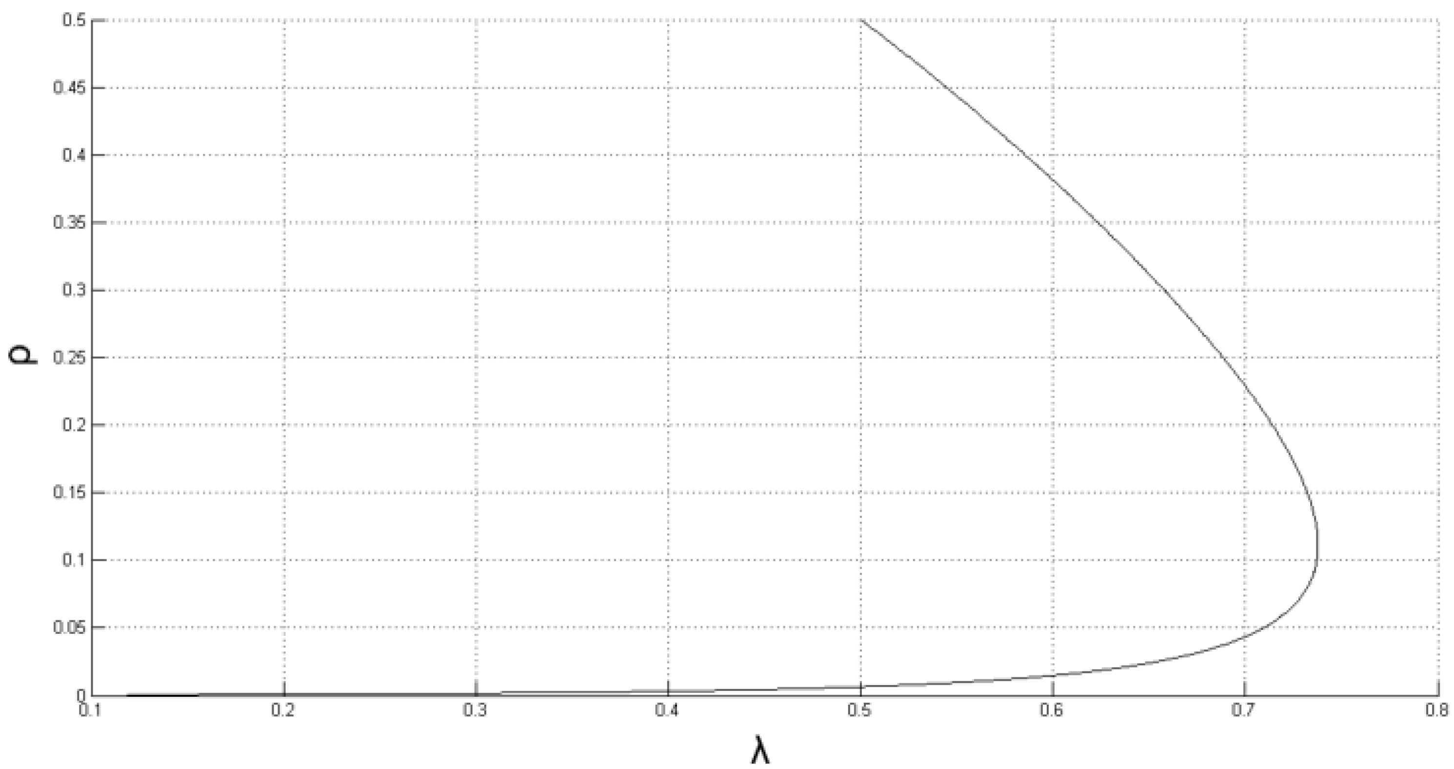
3.1. Dynamics I
Figure 1 depicts the trajectories of the system with either Equation (
2) or Equation (
3), the latter with small
effects, where it shows the trajectories. However, they are oscillating, asymptotically approaching the equilibrium
Locally stable, small shocks in the neighborhood of the steady states, or a sufficient liquidity provision policy, giving rise to small
disturbances only, will create local convergence. Economically, this is the case of self-stabilizing economic dynamics through liquidity buffers or liquidity policy, low
in economic terms. This is also called corridor stability (
Dimand 2005;
Leijonhufvud 1973). In this scenario, the large
is not operating locally and is not causing any notable destabilization.
3.2. Dynamics II
When large shocks occur along with significant effects from
and a large value of
v, it increases the risk of insolvency, as seen in
Figure 2. This often has occurred in terms of bank failures on the asset and/or liability side of banks if (
) there is no Federal Deposit Insurance Corporation (
) insurance for deposits, (
) banks did long-term lending, but short term borrowing, and (
) the value of capital assets (T-bonds), on the Banks asset side, was rapidly dropping due to interest rate rise. There were fast contagion effects among the depositors (and depositors of other banks). There were insufficient liquidity policies provided by the Federal Reserve
, and the Silicon Valley Bank
could not provide fast enough liquidity from the
using long-term assets as collateral.
In fact, in Dynamics II, if the diverging forces become strong enough to trigger significant disruptions, such as bank runs and contagion effects, it can lead to a situation where these forces cannot be adequately controlled through liquidity policy. Consequently, large effects from will occur, causing the trajectories of and to approach zero. This scenario entails an increased risk of insolvency, leading to actual insolvency, and with little liquidity policy coming to the rescue.
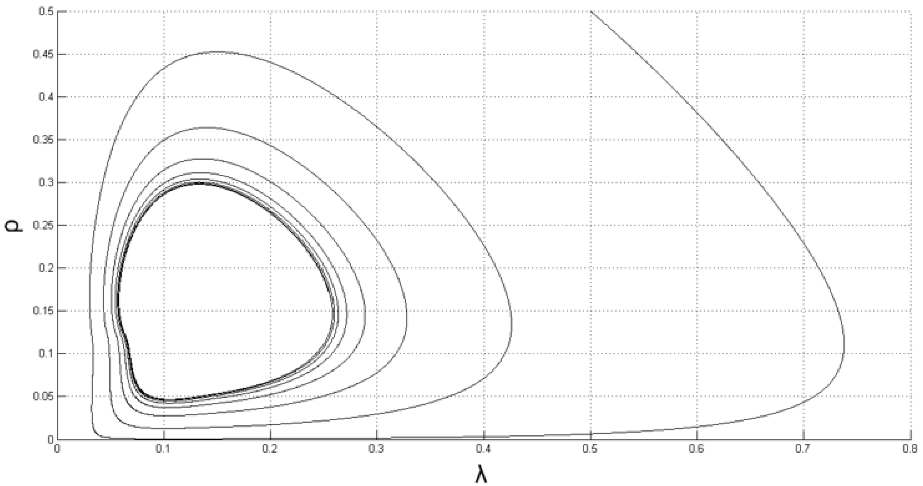
3.3. Dynamics III
However, if sufficient self-stabilizing forces and liquidity policies, such as lending against collaterals or extended deposit guarantees, are coming in, the disruptive and repelling force is weakening after large shocks; the responses can weaken the effects and the destabilizing forces, generating forces, leading to smaller fluctuations and limit cycles. Therefore, stability can mean stabilization toward stable cyclical fluctuations.
In the case of Dynamics III, self-stabilization and policies can prevent large shocks from moving the trajectory of
, and
does not go to the boundary to zero, as occurred in Dynamics II. However, now those stabilizing forces can come to the rescue, as displayed in
Figure 3. Contagion is prevented (through liquidity provision and guarantee of deposits) and central bank short-term borrowing is maintained; this way, firms can keep cash flows going, and the
does not go to zero.
In the next section, we will undertake a nonlinear econometric time series study to evaluate if such cycles, as in Dynamics III, can occur when we look at U.S. time-series data.
4. Estimation of Cycles Using Smooth Transition Regression Methodology
One of the major nonlinear time series methods to estimate nonlinear models, outlined in the previous section, is the regime change model. This encompasses the Markov Regime Switching model, which involves random switches between regimes, and the Threshold methodology, where pre-fixed thresholds dictate the occurrence of regime switches. There is also the Smooth Transition Regression methodology, which allows for smooth regime changes. For our empirical estimations using certain time periods of U.S. time-series data on liquidity and output or income (capital income) dynamics, we will use the methodology. In our empirical study, we thus focus on the implications of the endogenous banking liquidity dynamics resulting from the balance sheet dynamics of banks and study the endogenous liquidity of the corporate sector as the major driver of output and income.
4.1. Direct and Indirect Methods
In a more general context for such a regime-switching estimations method, there is also a
, which consists of discretizing the model, as given in
Section 2, which could lead to directly estimating its parameters. For a survey and comparison of the numerical accuracy of different discretization methods, see
Kloeden and Platen (
1992); for the local linearization procedure, see
Ozaki and Ozaki (
1989) and
Ozaki (
1985).
The second method, referred to as the in this context, is less model-dependent and instead focuses on approximating the continuous-time model using discrete-time state-dependent dynamics. In this approach, the lag structure is determined based on the data. Therefore, the direct method tests the model via parameters. In contrast, the indirect method could be considered a test of the presence of nonlinearities in the liquidity–output interaction without imposing restrictions directly implied by the model.
A model with a state-dependent reactions is, for example, the following van der Pol equation.
The term
represents a white noise shock, while
and
are constants. The second-order differential equations in
x can be estimated through direct procedures by employing, for example, the
; see
Ozaki and Ozaki (
1989). The van der Pol equation helps us describe the oscillatory behavior of the system ranging from simple harmonic motion to more complex, nonlinear oscillations depending on the value of the damping parameter
.
A generalization of this framework, called the
model, is elaborated by
Granger and Teräsvirta (
1993),
Luukkonen et al. (
1988a,
1988b),
Teräsvirta (
1994), and
Teräsvirta et al. (
2010). The
model is based on the idea that, unlike threshold autoregressive models, in both types of empirically oriented multiple equilibria models, the transitions between regimes, as steady-state rest points, may occur smoothly.
A single discrete time equation of the
model type can be written as follows.
Here,
is any variable postulated to govern the transition between regimes and
F is some bounded and continuous function. One widely used form of the
model is the
model characterized by a logistic function
F, i.e.,
with
. Another form is called the
model, where function
F is exponential, i.e.,
with
.
4.2. STR Methodology and Data
The empirical methodology of
involves several steps. The first step entails specifying a linear model that serves as the null hypothesis against which the linearity is tested. A test with power against both
and
involves testing
in the following auxiliary regression:
The above regression can also be used to determine the transition variable
by conducting the test for different variables. If linearity is rejected for several choices of
, the one with the smallest probability value is preferred as the transition variable. Given that the linearity hypothesis is rejected in favor of an
type of nonlinearity, one determines whether an
or
model is more appropriate by using the following sequence of nested hypotheses:
If the test of
has the smallest probability value, one chooses the
and otherwise chooses the
family. Estimation of a specified
model can then be undertaken by nonlinear least squares. For the following analysis, we employ the same data on the firms described above. The liquidity and the rate of return series have one unit root, as indicated by the augmented Dickey–Fuller tests. The data have been detrended and rendered stationary using the Hodrick–Prescott (HP) filter (with smoothness parameter 1600).
7The analysis covers the time period 1960.1–1988.4, utilizing quarterly data from the U.S. economy. The liquidity variable is defined as the ratio of liquid assets of the non-financial corporate business sector, obtained from the Flow of Funds Accounts (1994), to the capital stock for the same sector as estimated by Fair (1992).
8 The resulting series was seasonally adjusted before the analysis was conducted. As the income variable, we take the rate of return on capital, calculated as the flow of profits for the non-financial corporate business sector from the Flow of Funds Accounts, divided by the capital stock. Although the data were available for 1952.1–1991.4, the test and estimation period has been chosen as 1960.1–1988.4 for two reasons. First, before
, the series contains outliers that have been argued to favor the hypothesis of nonlinearities. Second, the period between
will later be used for out-of-sample forecasts. In both periods, liquidity provision is not operating under the central bank Taylor rule of monetary policy.
The main reason for choosing that time span is that, during that time period, the Taylor monetary policy rule was not yet being followed, and direct liquidity, for example, aiming at the growth rate of the money supply, was the ruling monetary policy variable. Our model is mainly concerned with the dynamics of the quantity of endogenous liquidity (and output or income), and the model does not much reference the role of the external interest rate. Even though since the beginning of 1990 the Taylor rule has become important, we believe that model dynamics with respect to endogenous liquidity could still be relevant because much of the liquidity is provided endogenously. In our data set, we are also bypassing banking liquidity, driven by the asset and liability side of banks’ balance sheets. We work directly with the endogenous liquidity available for the corporate sector.
5. The Linear Model
We use the following linear model as the reference model:
where
and
are polynomials in lag operator
L of degree 6, whereas
and
are of degree 8.
9 Using the above-mentioned data set, the estimated linear equation for liquidity is
10For the rate of return equation, we obtained
The standard diagnostic tests do not indicate any miss-specification for any of the equations. When simulated as a system, the linear model generates, as one would expect, convergent cycles and loses its forecasting ability soon after the iterations are started.
5.1. Linearity Tests and Model Specification
We postulate the following nonlinear equations as our alternatives to the linear ones above:
which would result in either a logistic smooth transition regression
model characterized by a logistic function F,
or an exponential smooth transition regression
model where function F is given by
The auxiliary equation to test for linearity is the same for both function forms of
F. We run the tests for each equation and various lags of both variables as potential transition variables.
Table 1 gives the results for the cases where the overall linearity tests have probability values
smaller than
. The probability value for
is
, for
it is
, and for
it is
.
The linearity hypothesis is rejected at a 6% significance level for the liquidity equation when the transition variable is
. It is rejected for several transition variables in the case of the rate of return equation, the most significant one arising when
is the transition variable. In addition, for both equations,
-type models are suggested. Hence, we have the following general specifications:
where
and
are both logistic functions.
5.2. Estimation and Diagnostics
The
models can be estimated using nonlinear least squares. Certain lags of both variables, which proved to be insignificant, were excluded to arrive at more parsimonious specifications. The estimated
equation for liquidity is
The model for liquidity performs better than its linear counterpart regarding static in-sample forecasting. The standard diagnostics do not indicate any miss-specification. The test for remaining nonlinearity indicates that the estimated model captures the nonlinearity well.
The transition parameter is
, which indicates a fast transition between what can be regarded as two regimes. The lower regime corresponds to that part of the state space where the rate of return is below
(which is slightly greater than the steady-state value of the rate of return), and the upper regime to the part where the rate of return is above that level. The dynamic properties of the model at different regions of the state space will be discussed later once the rate of return equation is also estimated. The
model for the rate of return is given by
where
denotes the linearity test with
as the transition variable. Concerning the static fit, the
equation for the rate of return again performs better than the linear one. Only the
test indicates miss-specification in the equation.
11 However, the estimated model still exhibits uncaptured nonlinearity at variable
of an
type. An appropriate strategy would be to re-estimate the equation using two transition variables,
and
, one entering with a logistic and the other as an exponential function.
12The transition parameter is much bigger for this equation, indicating an even faster transition between the lower (liquidity less than 0.0002—a value less than the steady state of the liquidity) and upper regimes (liquidity greater than 0.0002). Hence, the transition between regimes takes place much more quickly as a response to changes in liquidity (the financial variable) than to the rate of return (the real variable). This could be seen as an indication of the fact that firms adjust their behavior very fast as their liquidity gets closer and crosses over a critical level. The adjustment to the changes in the rate of return, however, takes place more smoothly.
To evaluate dynamic forecast performance, we first used the model estimated for the period 1960.1–1988.4 and calculated both the in-sample (1960.1–1988.4) and multi-step ahead forecasts (1989.1–1991.4). We also repeated this exercise using a Monte Carlo simulation rather than a deterministic one, where we shocked each equation in each period with a normally distributed random term (whose standard deviation is taken to be the standard error of the regression in respective models). We repeated this 1000 times and took the mean of the resulting simulations as our point forecasts.
13Using the deterministic simulation method, we found that the nonlinear model does a better job of simulating the rate of return within the sample. In contrast, the converse is true for the liquidity variable (see row 1960.1–1988.4 under Deterministic Simulations in
Table 2). However, the nonlinear model fares slightly better when we use the Monte Carlo simulations (row 1960.1–1988.4 under Monte Carlo Simulations). Out-of-sample forecast performance of the linear model is slightly better using the deterministic simulations. However, when we used Monte Carlo simulations, the nonlinear model performed better in forecasting the rate of return (row 1989.1–1991.4).
We also estimated the equations for the period 1960.1–1985.4 and conducted deterministic forecasts for the periods 1986.1–1991.4 and 1986.1–1988.4 (see rows 1986.1–1991.4 and 1986.1–1988.4 in
Table 2). Regarding the shorter period, we found that the nonlinear model has significantly better forecasting performance for both variables. However, for a longer period, the nonlinear model performs better only for the liquidity variable. Although the overall evidence seems to be inconclusive, on average, we can conclude that the linear model has a slightly better forecasting performance for the liquidity variable. In contrast, the nonlinear model has a significantly better forecast performance for the rate of return variable.
5.3. Evaluation of the Dynamic Properties
The theoretical model given by equation system (
3) implies through the term
thresholds for the behavior of the trajectories, generating Dynamics I, II, or III. Those possible dynamics will appear in a continuous time model. However, the empirical model has an important driving force, the logistic function
F of the discrete-time Equation (
13), which in the extreme takes values of zero and one but also takes infinitely more intermediate values. Due to this fact and due to the existence of many lags in the empirical model, it is not straightforward to establish a one-to-one correspondence between the regimes that appear in the theoretical and empirical models. However, we can roughly say that the specification of the empirical model, considering the limitations mentioned above, is similar to the theoretical model.
The steady-state values of the liquidity and the rate of return have been calculated numerically and found to be equal to
for liquidity and
for the rate of return.
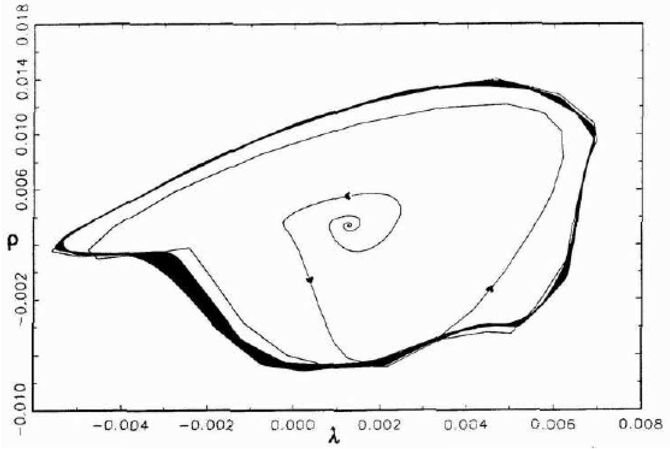
14 The system at the steady state has a pair of complex eigenvalues with a maximum modulus greater than unity, indicating local instability, as the Hopf bifurcation in the continuous time case would suggest. Thus here, too, in the discrete-time case, the fact that there exists one pair of complex eigenvalues whose real part is greater than unity indicates the possibility of a Hopf bifurcation taking place as some parameters change. If this is the case, then one would expect the emergence of a stable limit cycle.
15The system was simulated over extended periods (up to 15,000 iterations), and it was found that this is indeed the case (see
Figure 4). The simulations with different initial values inside and outside the limit cycle showed that this periodic motion was stable. The cycles have a period of approximately 26 quarters (or 6.5 years), which conforms well with the definition of the business cycle by the National Bureau of Economic Research (NBER).
16Thus, we can conclude that the dynamic interaction between liquidity and the rate of return on capital contains essential nonlinearities that lead to sustained fluctuations in both variables, even in the absence of exogenous shocks to the system. However, we could not detect corridor stability (as apparent from the fact that the steady state is locally unstable), which would require a more refined methodology, i.e., a model with multiple threshold variables in the dynamic equations.
6. Conclusions
Business cycles are often accompanied by waves of optimism and pessimism, resulting in fluctuating endogenous credit flows and liquidity. These factors interact with macroeconomic performance, including output and income flows. The recent crunch in credit flows and liquidity that originated in the banking system in the U.S., particularly in California, is throwing new light on the role of liquidity in business cycle dynamics.
In the normal path of the business cycle, liquidity and output (and income) mutually influence each other, and a mean reversion is generally achieved through market forces. When the degree of liquidity dissipation remains low, it does not significantly harm the economic dynamics. However, with larger liquidity dissipation due to bank runs and financial institution failures, followed by contagion effects, tipping points are likely to be reached, leading to major financial disruptions and economic contractions. These circumstances pose significant challenges for liquidity providers, such as corporations, the money market, commercial banks, and central banks. The latter usually react with a delay in letting the market work but then need to restore liquidity flows and trust in stability, avoiding further disruptions and meltdowns. This process involves a combination of positive and negative feedback effects from liquidity providers to corporations, banks, and households.
We explore three types of dynamics: a locally attracting one, resilience against any type of shock, and small or big shocks. However, dynamics following large shocks can lead to resilience breakers and long-term disruptions. To prevent such disruptions, policy measures can be implemented to induce dynamics among driving variables that interact to generate persistent cycles, with the support of timely policy actions. We empirically test the latter type of dynamics in a nonlinear model of the liquidity–macro interaction and econometrically explore those dynamic feedback features for the U.S. economy. Guided by a theoretical model, we use nonlinear econometrics of a Smooth Transition Regression () type to study those features by including further policy measures such as regulation and monitoring guidelines and institutional enforcement of rules.
Our empirical analysis has shown that we can use a continuous time regime change model to study state-dependent reactions and regime changes in cross effects between liquidity–macro variables, i.e., the direct method (Euler scheme and Ozaki’s local linearization method), as well as a discrete-time version, which we call the indirect method (
methodology).
17 Both the application of the Euler method as well as the local linearization procedure of Ozaki are encouraging. Although the first is easier to apply, it may generate instability. The latter is more difficult to employ since the number of observations to be used for a higher dimensional state space is quite large, and the computation is very time-consuming. Although the direct method revealed some expected dynamic behavior, such as regime change behavior, when estimated, lag effects and delay effects do not seem to play an important role. For the latter, see
Chen et al. (
2022).
Applying the
methodology is particularly interesting. The data reveals that a linear model also fits well and demonstrates a convergent behavior, suggesting a stable steady state.
18 In other words, if one assumes a linear representation of the data, the system would be considered stable around the steady state. Any fluctuations observed would then be attributed to external shocks or factors. As standard models often exhibit, one would always observe a mean reversion behavior of the variables. However, a regime change model, which we claim is a better representation of the data, reveals that the actual dynamics of the system are characterized by a locally unstable steady state contained by stable outer regions.
19Regime change models are capable of exploring and answering more intriguing questions that have been extensively discussed in theoretical literature but have lacked empirical analysis. The results of this paper provide evidence in support of a particular class of credit and output interaction models characterized by an unstable steady state, regime shifts, and asymmetric responses to shocks. This encourages further work to examine regime changes in other macroeconomic relationships, for example, in relations between stock market data and output (see
Semmler and Koçkesen 2017) or exchange rate data and output. Time series models based on thresholds seem to be particularly useful in this endeavor.
Higher dimensional models can also be studied where such thresholds exist, not as threshold points but as threshold surfaces. Moreover, existing work shows that the complex dynamics can generate steady states as a trapping region, as bad attractors, where the dynamics nearby can be trapped in a low-level equilibrium with features of persistent traps, as seen in
Semmler et al. (
2023). They provide examples of this type arising from severe financial and climate disasters with extensive disruptions from normal business cycle dynamics, even for longer time periods.
Following the global financial crisis, central banks increasingly relied on liquidity facilities to manage cross-currency liquidity effectively. Therefore, it is natural to question the factors contributing to another potential financial crisis fifteen years after the previous one. In this context,
Albrizio et al. (
2023) found that introducing the European Central Bank’s
euro liquidity lines led to a decrease in borrowing premiums for foreign entities.
20Though our model might be viewed as depicting more of the earlier time when monetary policy was not guided by the Taylor rule, concerning the liquidity dynamics, it may be worth making a remark on the collapse of
in California, and the situation close to an economic-wide disruption could be related to our model. It was, to a great extent, caused by its failure to diversify its investments, which ultimately led to its insolvency and triggered bank runs. The
had lent money to the Federal government by purchasing long-term bonds. However, when depositors sought to withdraw their funds, the
could not repay, leading to a liquidity crisis that became an insolvency problem. The result was a destructive cycle where the outflow of money from
forced the bank to sell bonds at a loss, further exacerbating their financial losses and causing more depositors to withdraw their funds. The absence of active liquidity policies by the monetary authority to prevent such banking crises and minimize losses during asset sales by depositors accelerates the run. It is, therefore, crucial to establish liquidity buffers provided by the Federal Reserve, such as collateralized short-term lending to banks. However, this also did not seem to have been effective during the
episode. Stricter government regulations and more forceful liquidity provisions are necessary to prevent future bank failures.
21It is also important to note that the quick escalation of interest rates may have unanticipated economic ramifications. This is exemplified by the ongoing debate surrounding the underlying causes of the current inflation, which can be attributed to various sources of disruptions. If inflation is primarily caused by excessive aggregate demand, it is appropriate to implement monetary policy measures, such as tightening, to reduce overall demand. However, if inflation is mainly driven by supply-side factors, a more targeted approach is needed, which includes implementing fiscal policies that address the constraints on the supply side. A combination of factors seems to have contributed to the recent inflationary conditions, but empirical evidence sheds light on its primary drivers.
Stiglitz and Regmi (
2023) demonstrated that the present inflation is not a result of an excess demand; specifically, it is not caused by excessive spending during the pandemic but is rather due to disruptions in the supply side, primarily caused by the pandemic (such as chip shortages) and the war in Ukraine, along with changes in demand within specific sectors. While the economy appreciates the restoration of interest rates to a more customary level, which serves to mitigate distortions resulting from prolonged, abnormally low rates, an excessive and swift increase in interest rates presents the potential for a deleterious deceleration of the economy with negligible effects on inflation unless a substantial downturn is experienced.
In essence, mistakes were certainly made, such as a lack of proactive monetary policy before the financial crisis, delayed termination of quantitative easing afterward, and slower withdrawal of monetary support in 2021. However, it is doubtful that any of these measures would have led to a fine-tuning and smooth mean reversion; quite commonly, boom–bust cycles are observable, and sometimes disruptions occur.


