Article

When It Counts—Econometric Identification of the Basic Factor Model Based on GLT Structures

by
Sylvia Frühwirth-Schnatter
1,
Darjus Hosszejni
1,* and
Hedibert Freitas Lopes
2,3
1
Department of Finance, Accounting, and Statistics, WU Vienna University of Economics and Business, 1020 Vienna, Austria
2
School of Mathematical and Statistical Sciences, Arizona State University, Tempe, AZ 85281, USA
3
Insper Institute of Education and Research, São Paulo 04546-042, Brazil
*
Author to whom correspondence should be addressed.
Econometrics 2023, 11(4), 26; https://doi.org/10.3390/econometrics11040026
Submission received: 24 February 2023 / Revised: 29 October 2023 / Accepted: 1 November 2023 / Published: 20 November 2023
(This article belongs to the Special Issue High-Dimensional Time Series in Macroeconomics and Finance)

Abstract

:
Despite the popularity of factor models with simple loading matrices, little attention has been given to formally address the identifiability of these models beyond standard rotation-based identification such as the positive lower triangular (PLT) constraint. To fill this gap, we review the advantages of variance identification in simple factor analysis and introduce the generalized lower triangular (GLT) structures. We show that the GLT assumption is an improvement over PLT without compromise: GLT is also unique but, unlike PLT, a non-restrictive assumption. Furthermore, we provide a simple counting rule for variance identification under GLT structures, and we demonstrate that within this model class, the unknown number of common factors can be recovered in an exploratory factor analysis. Our methodology is illustrated for simulated data in the context of post-processing posterior draws in sparse Bayesian factor analysis.

1. Introduction

Ever since the pioneering work of Thurstone (1935, 1947), factor analysis has been a popular method to model the covariance matrix Ω of correlated, multivariate observations y t of dimension m (see, e.g., Anderson (2003) for a comprehensive review). Assuming r uncorrelated factors in a basic factor model, for instance, yields the representation Ω = Λ Λ + Σ 0 , with a m × r factor loading matrix Λ and a diagonal matrix Σ 0 . This considerable reduction in the number of parameters compared to the m ( m + 1 ) / 2 parameters of an unconstrained covariance matrix is the main motivation for applying factor models to covariance estimation, especially if m is large (see, among many others, Fan et al. (2008)). In addition, shrinkage estimation has been shown to lead to very efficient covariance estimation (see, for example, Kastner (2019) in Bayesian factor analysis and Ledoit and Wolf (2020) in a non-Bayesian context).
In numerous applications, factor analysis reaches beyond covariance modeling (see, among many others, Forni et al. (2009) in the context of structural factor models). From the very beginning, the goal of factor analysis has been to extract the underlying loading matrix Λ to understand the driving forces behind the observed correlation between the measurements (see, e.g., Owen and Wang (2016) for a recent review). However, also in this setting, the only source of information is the observed covariance of the data, making the decomposition of the covariance matrix Ω into the cross-covariance matrix Λ Λ and the variance Σ 0 of the idiosyncratic errors more challenging than estimating only Ω itself.
A huge amount of literature, dating back to Koopmans and Reiersøl (1950) and Reiersøl (1950), has addressed this problem of identification which can be resolved only by imposing additional structure on the factor model. Anderson and Rubin (1956) consider two kinds of conditions for identification. The first problem, also known as solving rotational invariance, aims at identifying Λ , assuming that Λ Λ is determined uniquely. This problem has received considerable attention in econometrics, statistics, and machine learning. The most popular condition for solving rotational invariance is to consider positive lower triangular (PLT) loading matrices (see, e.g., Geweke and Zhou (1996); Lopes and West (2004); West (2003)), although other strategies have been put forward (see, e.g., Neudecker (1990), Bai and Ng (2013), Aßmann et al. (2016), Chan et al. (2018), and Williams (2020)). In related strands, Anderson et al. (2016) examine the generic identifiability of dense vector autoregressive systems with mixed frequencies, and their theory is also applicable to static factor models.
In the second problem, Anderson and Rubin (1956) consider conditions for variance identification, i.e., unique identification of Λ Λ and Σ 0 assuming that the covariance matrix Ω = Λ Λ + Σ 0 arises from a basic factor model. Examples in Bartholomew (1987), for instance, show that two different models could imply the same covariance matrix. Sufficient conditions for ensuring variance identification have received much less attention than the first problem. Conditions include the row-deletion property (Anderson and Rubin 1956) and a simple counting rule for the number of non-zero loading in each column of the factor loading matrix in the context of dedicated factor models (Conti et al. 2014); see also Bekker (1989) for related work.
In this work, we discuss conditions for identification based on ordered and unordered generalized lower triangular (GLT) structures which relax the PLT condition, see Figure 1 for illustration. This concept was first introduced in the unpublished work by Frühwirth-Schnatter and Lopes (2018) as part of an MCMC sampler for sparse Bayesian factor analysis where the number of factors is unknown. In the present paper, GLT structures are given a full and comprehensive mathematical treatment. It will be proven that GLT structures simultaneously address rotational invariance and variance identification in factor models. Variance identification relies on a counting rule for the number of non-zero elements in the loading matrix Λ , which is a sufficient condition that extends the previous work by Sato (1992) and Conti et al. (2014).
In addition, we show that unordered GLT structures are useful in exploratory factor analysis where the factor dimension r is unknown. Identification of the number of factors in applied factor analysis is a notoriously difficult problem for many latent factor models, with considerable ambiguity about which method works best, be it BIC-type criteria for approximate factor models (Bai and Ng 2002), marginal likelihoods for basic factor models (Lopes and West 2004), techniques from Bayesian non-parametrics involving infinite-dimensional factor models (Bhattacharya and Dunson 2011; Legramanti et al. 2020; Ročková and George 2017) or more heuristic procedures for dynamic factor models (Kaufmann and Schumacher 2019). Imposing an unordered GLT structure in exploratory factor analysis allows us to identify the true factor dimension by spotting spurious columns in a possibly overfitting model and to identify the true loading matrix Λ and the matrix Σ 0 .
The theoretical results of the present paper are exploited in related work. Relying on ordered and unordered GLT structures, Frühwirth-Schnatter et al. (2023) develop an efficient reversible jump MCMC sampler for sparse Bayesian factor analysis under very general shrinkage priors when the number of factors is unknown and use the counting rules introduced in this paper for postprocessing the posterior draws.
The current paper is structured as follows. Section 2 reviews the role of identification in a basic factor model using illustrative examples. Section 3 introduces ordered and unordered GLT structures, proves identification for simple GLT structures, and shows that any full column-rank unconstrained loading matrix has a unique representation as a GLT matrix. Section 4 addresses variance identification under GLT structures. Section 5 discusses exploratory factor analysis under unordered GLT structures and addresses additional identification problems that arise in a basic factor model when the number of factors is unknown. Section 7 presents illustrative applications to simulated and empirical data. Section 8 concludes.

2. The Basic Factor Model

2.1. Model Definition

Let ( y 1 , , y T ) be a sequence of observations, where y t = ( y 1 t , , y m t ) for t = 1 , , T is a vector of m measurements assumed to arise from a multivariate normal distribution, y t N m 0 , Ω , with zero mean and covariance matrix Ω . In factor analysis, the correlation among the measurements in y t is assumed to be driven by a latent r-variate random variable f t = ( f 1 t , , f r t ) , the so-called common factors, through the following observation equation:
y t = Λ f t + ϵ t ,
where the m × r matrix Λ containing the factor loadings Λ i j is of full column rank, rk ( Λ ) = r , equal to the factor dimension r.
In the present paper, we focus on the so-called basic factor model where the observations ( y 1 , , y T ) are assumed to be iid. Furthermore, the vector ϵ t = ( ϵ 1 t , , ϵ m t ) accounts for the independent, idiosyncratic variation in each measurement and is distributed as ϵ t N m 0 , Σ 0 , with Σ 0 = Diag σ 1 2 , , σ m 2 being a positive definite diagonal matrix. The common factors are orthogonal, meaning that f t N r 0 , I r , and independent of ϵ t . In this case, the observation Equation (1) implies the following covariance matrix Ω , when we integrate with respect to the latent common factors f t :
Ω = Λ Λ + Σ 0 .
Finally, the model assumes independence of f t and f s , f t and ϵ s , and ϵ t and ϵ s for all s t . All cross-sectional dependence among the m measurements in y t is explained through the latent common factors and the off-diagonal elements of Λ Λ define the marginal covariance between any two measurements y i 1 , t and y i 2 , t :
Cov ( y i 1 , t , y i 2 , t ) = Λ i 1 , Λ i 2 , ,
where Λ i , is the ith row of Λ . Consequently, we will refer to Λ Λ as the cross-covariance matrix. Since the number of factors, r, is often considerably smaller than the number of measurements, m, (2) can be seen as a parsimonious representation of the dependence between the measurements, with considerably fewer parameters in the factor loading matrix Λ than the m ( m 1 ) / 2 off-diagonal elements in an unconstrained covariance matrix  Ω .

2.2. Loading Matrices with a Simple Structure

The factor loading matrices given in Figure 1 are examples of simple structures in the sense specified by Thurstone (1947), where each variable loads only on specific factors and factors affect only a subset of variables. In traditional factor analysis, after estimating an identified matrix of loadings, factors are rotated so as to enhance a simple structure, the most popular procedure being Varimax (see, e.g., Magnus and Neudecker (2019, sct. 17.14)). In sparse Bayesian factor analysis, which will be discussed in more detail in Section 6.1, priors are chosen that encourage automatic rotation to a simple structure (see, e.g., Ročková and George (2017)).
Subsequently, we will make use of a representation of a factor loading matrix Λ with a simple structure called the sparsity matrix. The sparsity matrix δ is a binary indicator matrix of 0 s and 1 s of the same dimension as Λ and contains the information which elements of a factor loading matrix with a simple structure are equal to 0 and which elements are unconstrained, i.e., if δ i j = 0 , then Λ i j = 0 , while Λ i j R if δ i j = 1 .
The sparsity matrix δ contains a lot of information about the structure of Λ (see the left-hand matrix in Figure 1 for illustration). In total, six factors are needed to fully explain the variation in these 22 measurements. The fifth row contains only zeros, which tells us that measurement y 5 t is uncorrelated with the remaining measurements, since Cov ( y i t , y 5 t ) = 0 for all i 5 . The measurements 1, 3, 10, 11, 14, and 17 each constitute a new factor. Hence, the variation in the first nine measurements can be explained by at most two factors which also load on some (but not all) of the remaining measurements. The rows which constitute a new factor will play an instrumental role for identification in the present paper. More specifically, the sparsity matrix on the left hand side tells us that the underlying loading matrix Λ has an ordered GLT structure, while the matrix in the middle is one of many unordered GLT structures that can be derived from Λ . The sparsity matrix on the right hand side indicates that the loading matrix Λ has the commonly applied PLT structure where the first six measurements lead the six factors. Ordered and unordered GLT structures will be discussed in full details in Section 3.

2.3. A Brief Review of Identification When the Number of Factors Is Known

Since the factors f t are unobserved, the only information available to estimate Λ and Σ 0 is the covariance matrix Ω , which creates well-known identification issues for the basic factor model. Consider, for example, the following factor loading matrix Λ and all loading matrices β = Λ P α b defined as a rotation of Λ :
Λ = λ 11 0 λ 21 0 λ 31 0 λ 41 λ 42 0 λ 52 0 λ 62 , P α b = cos α ( 1 ) b sin α sin α ( 1 ) b cos α , β = β 11 β 21 β 21 β 22 β 31 β 32 β 41 β 42 β 51 β 52 β 61 β 62 .
Then, for any α [ 0 , 2 π ) and b { 0 , 1 } , the factor loading matrix β yields the same cross-covariance matrix for y t as Λ :
β β = Λ P α b P α b Λ = Λ Λ .
The rotational invariance apparent in (5) holds for any basic factor model (1), as is easily verified. Take any r × r rotation matrix P (i.e., P P = I r ) and define the basic factor model
f t N r 0 , I r , y t = β f t + ϵ t , ϵ t N m 0 , Σ 0 ,
where β = Λ P and f t = P f t . Obviously, both models imply the same covariance Ω , given by (2). Hence, without imposing further conditions, Λ is in general not identified from the cross-covariance matrix Λ Λ . The usual way of dealing with this rotational invariance is to constrain Λ in such a way that the only possible rotation is the identity P = I r . For orthogonal factors, at least r ( r 1 ) / 2 restrictions on the elements of Λ are needed to eliminate rotational indeterminacy (Anderson and Rubin 1956).
As Anderson and Rubin (1956) point out, additional insight can be gained by comparing the number of parameters in Ω , namely m ( m + 1 ) / 2 , with the number of parameters in the pair ( Λ , Σ 0 ) , namely m ( r + 1 ) . If r ( r 1 ) / 2 restrictions are imposed to eliminate rotational indeterminacy, this yields the necessary condition ( m r ) 2 > m + r (see also Anderson (2003, sct. 14.2.2)). However, this condition is by no means sufficient for identification, as will be illustrated in Example (9) below, where m = 5 and r = 2 satisfies this condition, but identifiability fails.
A rigorous approach toward the identification of factor models was first offered by Anderson and Rubin (1956). Assume that a pair of parameters ( Λ , Σ 0 ) , where Λ is an m × r matrix and Σ 0 is a positive definite diagonal matrix, satisfying (2) is given. Let ( β , Σ ) , where β is an m × r matrix and Σ is a positive definite diagonal matrix, be another pair of parameters satisfying (2). Then,
Ω = β β + Σ = Λ Λ + Σ 0 ,
and both pairs imply the same Gaussian distribution y t N m 0 , Ω for every possible realization y t . For an identified model, it would follow that the two pairs of parameters are identical, i.e., β = Λ and Σ = Σ 0 . However, as discussed above, identification can be achieved for a basic factor model only by imposing conditions on Λ and Σ 0 .
Anderson and Rubin (1956) consider two kinds of conditions for identification. First, they consider conditions assuming that Λ Λ and Σ 0 are determined uniquely. According to their Lemma 5.1, any alternative loading matrix β which satisfies β β = Λ Λ (while Σ = Σ 0 ) and, consequently, implies the same covariance matrix Ω as Λ , is an orthogonal rotation P of Λ , i.e., β = Λ P . Conditions are then imposed on the structure of Λ to solve this rotational invariance problem (see Section 2.4 for details). Second, they consider conditions that ensure that Λ Λ and Σ 0 are, indeed, determined uniquely. In their Theorem 5.1, they formulate a row-deletion property as a sufficient condition to resolve the variance identification problem and ensure unique identification of the variance decomposition in (2) (see Section 2.5 for details). The literature on factor analysis often reduces the identification of factor models to the first problem; however, as we will argue in the present paper, variance identification is equally important, in particular for loading matrices with a simple structure.

2.4. Conditions Resolving Rotational Invariance

Let us assume that variance identification holds and Λ Λ and Σ 0 are determined uniquely from Ω . By far, the most popular constraints to deal with rotational invariance are positive lower triangular (PLT) loading matrices, where the upper triangular part is constrained to be zero and the main diagonal elements Λ 11 , , Λ r r of Λ are strictly positive.1 The corresponding sparsity matrix δ also exhibits a PLT structure (see the right-hand side of Figure 1 for illustration).
Despite its popularity, the PLT structure is restrictive, as outlined already by Jöreskog (1969). Let β β be an arbitrary cross-covariance matrix with factor loading matrix β . A PLT representation for β β is possible if the top r rows of β are linearly independent, or, equivalently, if a rotation matrix P exists such that β can be rotated into a PLT matrix Λ = β P . However, as example (4) illustrates, this is not necessarily the case. Obviously, Λ is not a PLT matrix, since Λ 22 = 0 . Any of the possible rotations β = Λ P α b have non-zero elements above the main diagonal and are not PLT matrices either. This example demonstrates that the PLT representation is restrictive. To circumvent this problem in Example (4), one could reorder the measurements in an appropriate manner. However, in applied factor analysis, such an appropriate ordering is typically not known in advance and the choice of the first r measurements is an important modeling decision under PLT constraints (see, e.g., Lopes and West (2004) and Carvalho et al. (2008)).
An alternative identification condition, also dating back to Anderson and Rubin (1956), is assuming diagonality of Λ Σ 0 1 Λ and requires the corresponding diagonal elements d 1 , , d r to be different. In practice, however, weak identifiability might occur if some of the elements d 1 , , d r are similar, even if not equal. Furthermore, in an attempt to formalize the criteria for simplicity of Thurstone (1947), Reiersøl (1950) put forward a condition which requires a minimum of r zero factor loadings in each column. However, this condition rules out the existence of a “market” factor that loads on all measurements as for the financial returns in our empirical case study in Section 7.2.
In Section 3, we discuss a new identification strategy to resolve rotational invariance in factor models based on the concept of generalized lower triangular (GLT) structures. Loosely speaking, GLT structures generalize PLT structures by freeing the position of the first non-zero factor loading in each column (see the examples in Figure 1 and the loading matrix Λ in (4)). Consequently, the use of GLT structures for rotational identification does not imply that the first r rows of the loading matrix are linearly independent, as the use of PLT structures would, but only that there exist r linearly independent rows in Λ . This weakened condition hints at a wider applicability of GLT structures compared to PLT structures. In particular, we show in Section 3.2 that a unique GLT structure Λ can be identified from any cross-covariance matrix β β , provided that variance identification holds and, consequently, β β itself is identified. Even if β β is obtained from a loading matrix β that does not take the form of a GLT structure, such as the matrix β in (4), we show that an orthogonal matrix G exists which represents β = Λ G as a rotation of an ordered GLT structure Λ and defines the unique rotation Λ = β G of β into GLT. Hence, the GLT representation is unrestrictive in the sense of Anderson and Rubin (1956) and Jöreskog (1969), and is a generic way to resolve rotational invariance for any factor loading matrix.

2.5. Conditions for Variance Identification

Conditions that resolve rotational invariance typically take variance identification, i.e., identification of Λ Λ , for granted (see, e.g., Geweke and Zhou (1996)). Variance identification refers to the problem that the idiosyncratic variances σ 1 2 , , σ m 2 in Σ 0 are identified only from the diagonal elements of Ω , as all elements in the cross-variance matrix Λ Λ are independent of the σ i 2 s (see again (3)). To achieve variance identification of σ i 2 from Ω i i = Λ i , Λ i , + σ i 2 , all factor loadings have to be identified solely from the off-diagonal elements of Ω . Variance identification, however, is easily violated, as the following examples illustrate.
Let us consider a factor model with the following loading matrix (also known as a dedicated factor model; see, e.g., Conti et al. 2014):
Λ = λ 11 0 λ 21 0 λ 31 0 0 λ 42 0 λ 52 0 λ 62 .
The corresponding covariance matrix Ω is given by:
Ω = λ 11 2 + σ 1 2 λ 11 λ 21 λ 11 λ 31 λ 11 λ 21 λ 21 2 + σ 2 2 λ 21 λ 31 0 λ 11 λ 31 λ 21 λ 31 λ 31 2 + σ 3 2 λ 42 2 + σ 4 2 λ 42 λ 52 λ 42 λ 62 0 λ 42 λ 52 λ 52 2 + σ 5 2 λ 52 λ 62 λ 42 λ 62 λ 52 λ 62 λ 62 2 + σ 6 2 .
Let us assume that the sparsity matrix δ of Λ is given (i.e., we know which elements in (7) are zero), but the specific values of the unconstrained loadings ( λ 11 , , λ 62 ) are unknown. An interesting question is the following. Knowing Ω and δ , can the unconstrained loadings λ 11 , , λ 62 and the idiosyncratic variances σ 1 2 , , σ m 2 be identified uniquely? Given Ω , the three nonzero covariances Cov ( y 1 t , y 2 t ) = λ 11 λ 21 , Cov ( y 1 t , y 3 t ) = λ 11 λ 31 and Cov ( y 2 t , y 3 t ) = λ 21 λ 31 are available to identify the three factor loadings ( λ 11 , λ 21 , λ 31 ) . Similarly, the three nonzero covariances Cov ( y 4 t , y 5 t ) = λ 42 λ 52 , Cov ( y 4 t , y 6 t ) = λ 42 λ 62 and Cov ( y 5 t , y 6 t ) = λ 52 λ 62 are available to identify the factor loadings ( λ 42 , λ 52 , λ 62 ) . Hence, variance identification holds. However, when we remove the last measurement from the loading factor matrix defined in (7), we obtain
Λ = λ 11 0 λ 21 0 λ 31 0 0 λ 42 0 λ 52 ,
and the corresponding covariance matrix Ω reads:
Ω = λ 11 2 + σ 1 2 λ 11 λ 21 λ 11 λ 31 λ 11 λ 21 λ 21 2 + σ 2 2 λ 21 λ 31 0 λ 11 λ 31 λ 21 λ 31 λ 31 2 + σ 3 2 λ 42 2 + σ 4 2 λ 42 λ 52 0 λ 42 λ 52 λ 52 2 + σ 5 2 .
While the three factor loadings ( λ 11 , λ 21 , λ 31 ) are still identified from the off-diagonal elements of Ω as before, variance identification of σ 4 2 and σ 5 2 fails. Since Cov ( y 4 t , y 5 t ) = λ 42 λ 52 is the only non-zero element that depends on the loadings λ 42 and λ 52 , infinitely many different parameters ( λ 42 , λ 52 , σ 4 2 , σ 5 2 ) imply the same covariance matrix Ω .
From these considerations, it is evident that a minimum of three non-zero loadings is necessary in each column to achieve variance identification, a condition which dates back to Anderson and Rubin (1956). At the same time, this condition is not sufficient. For illustration, consider the rotation β = Λ P α b of the loading matrix Λ in (9) with α { 0 , π 2 , π , 3 π 2 } , where all elements of the corresponding sparsity matrix are equal to 1. Although each column of β has six non-zero elements, variance identification obviously does not hold.
For more general loading matrices, variance identification is not as easily verified as for these examples and we rely in the present paper on the row-deletion property introduced by Anderson and Rubin (1956).
Definition 1
(Row-deletion property AR (Anderson and Rubin 1956)). An m × r factor loading matrix Λ satisfies the row-deletion property if the following condition is satisfied: whenever an arbitrary row is deleted from Λ, two disjoint submatrices of rank r remain.
Anderson and Rubin (1956, Theorem 5.1) prove that the row-deletion property is a sufficient condition for the identification of Λ Λ and Σ 0 from the marginal covariance matrix Ω given in (2). For any (not necessarily GLT) factor loading matrix Λ , the row-deletion property AR can be trivially tested by a step-by-step analysis, where every single row of Λ is sequentially deleted and the two distinct submatrices are determined from examining the remaining matrix (Hayashi and Marcoulides 2006). However, this procedure is inefficient in higher dimensions and simpler conditions for verifying variance identification under the row-deletion property AR are warranted.
The literature provides necessary conditions for AR that are based on counting the number of non-zero factor loadings in Λ , such as: for every nonsingular r-dimensional square matrix G , the matrix β = Λ G contains at least three nonzero factor loadings in each column, and at least five nonzero factor loadings in each pair of columns (Anderson and Rubin 1956). Sato (1992, Theorem 3.3) extends these necessary conditions in the following way: every subset of 1 q r columns of β = Λ G contains at least 2 q + 1 nonzero factor loadings for every nonsingular matrix G . We call this the 3579 counting rule for obvious reasons.
For illustration, apply the 3579 counting rule to all rotations β = Λ P α b of the loading matrix Λ in Example (7) for which we already verified variance identification. We find that the counting rules are satisfied for all rotations β , and one might wonder if the 3579 counting rule can also lead to a sufficient criterion for variance identification under AR.
Sufficiency of counting rules was proven by Conti et al. (2014) in the context of a dedicated factor model, where the factor loading matrix Λ has a perfect simple structure, i.e., each measurement y i t loads on at most one factor, as in (7) and (9); however, the sparsity matrix δ , i.e., the exact position of the non-zero elements, is unknown. Conti et al. (2014) consider a dedicated factor model with correlated factors, f t N r 0 , R , and prove that the following conditions are both necessary and sufficient for uniqueness of the variance decomposition: the correlation matrix R is of full rank, rk ( R ) = r , and each column of Λ contains at least three nonzero loadings.
In the present paper, we aim for simple structures with potentially more than one non-zero loading in each row and generalize this work to basic factor models with orthogonal factors. We impose a GLT condition on the loading matrices Λ and provide sufficient conditions for variance identification in Section 4. These conditions are formulated as counting rules for the sparsity matrix δ of Λ . More specifically, if the 3579 counting rule of Sato (1992, Theorem 3.3) holds for δ , then this is a sufficient condition for the row-deletion property AR and, consequently, for variance identification, except for a set of measure 0.
Assuming a GLT structure also avoids the need to check the counting rule for all rotations of a given loading matrix. For illustration, we return to example (9) and use the counting rule of Sato (1992) to verify variance identification for β . If no condition to resolve rotational invariance is imposed on β , then the counting rule of Sato (1992) has to be checked not only for β , but for all rotations β G or, equivalently, for all possible rotations Λ P α b of Λ . Nearly all rotations have five non-zero rows and do not violate the counting rules, except for the eight rotations where ( α , b ) { 0 , π 2 , π , 3 π 2 } × { 0 , 1 } leads to trivial rotations of Λ :
λ 11 0 λ 21 0 λ 31 0 0 λ 42 0 λ 52 λ 11 0 λ 21 0 λ 31 0 0 λ 42 0 λ 52 λ 11 0 λ 21 0 λ 31 0 0 λ 42 0 λ 52 λ 11 0 λ 21 0 λ 31 0 0 λ 42 0 λ 52 0 λ 11 0 λ 21 0 λ 31 λ 42 0 λ 52 0 0 λ 11 0 λ 21 0 λ 31 λ 42 0 λ 52 0 0 λ 11 0 λ 21 0 λ 31 λ 42 0 λ 52 0 0 λ 11 0 λ 21 0 λ 31 λ 42 0 λ 52 0 .
On the other hand, if we impose an unordered GLT structure on β , then the set of all possible rotations β G reduces to the eight permutations in (10) and lack of variance identification can be verified by applying the counting rule of Sato (1992) to a single one of them.

3. Solving Rotational Invariance through GLT Structures

3.1. Ordered and Unordered GLT Structures

In this work, we introduce a new identification strategy to resolve rotational invariance based on the concept of generalized lower triangular (GLT) structures. Throughout this section, we assume that variance identification holds and Λ Λ and Σ 0 are uniquely determined from  Ω . First, we introduce the notion of pivot rows of a factor loading matrix  Λ .2
Definition 2
(Pivot rows). Consider an m × r factor loading matrix Λ with r non-zero columns. For each column j = 1 , , r of Λ, the pivot row l j is defined as the row index of the first non-zero factor loading in column j, i.e., Λ i j = 0 , i < l j and Λ l j , j 0 . The factor loading Λ l j , j is called the leading factor loading of column j.
Conditions on the pivot rows define different structures on the factor loading matrix. If the pivot rows lie on the main diagonal, i.e., ( l 1 , , l r ) = ( 1 , , r ) , then the factor loading matrix Λ exhibits a PLT structure and the leading factor loadings are equal to Λ j j for all columns j = 1 , , r . GLT structures also require the pivot rows ( l 1 , , l r ) to be pairwise distinct, but impose less stringent conditions on their position than a PLT structure. We will distinguish between two types of GLT structures, namely ordered and unordered GLT structures. In the first case, the pivots l 1 < < l r are ordered by size (see Definition 3), whereas they may take arbitrary positions ( l 1 , , l r ) for unordered GLT structures, as long as they are pairwise distinct (a more formal definition is given below). Examples of all three structures are displayed in Figure 1 for a model with r = 6 factors. Obviously, GLT structures contain the PLT structure as the special case where l j = j for j = 1 , , r .
Definition 3
(Ordered GLT structures). An m × r factor loading matrix Λ with full column rank r has an ordered GLT structure if the pivot rows l 1 , , l r of Λ are ordered, i.e., l 1 < < l r , and the leading factor loadings are positive, i.e., Λ l j , j > 0 for j = 1 , , r .
Since the “diagonal” loadings Λ j j are allowed to be zero for an ordered GLT structure, measurements different from the first r ones may lead the factors. For each factor j, the leading variable is the response variable y l j , t corresponding to the pivot row l j . From a mathematical viewpoint, one could argue that the m measurements y 1 t , , y m t can be rearranged such that a PLT structure holds and the diagonal of the first r rows of Λ has non-zero elements. However, in practice, it is not obvious which measurements are able to constitute a new factor; in particular, if we expect the loading matrix Λ to exhibit a simple structure, but the measurements have no natural grouping. Even if such a grouping exists, rearranging the measurements might be challenging, if more than one factor is needed to explain the group-specific covariance.
As opposed to PLT, under GLT structures, we may learn from the data whether the ith row of the loading matrix is linearly independent of the previous rows 1 to i 1 . Only in this case, the measurement y i t constitutes an additional factor and row i defines the next pivot. In the empirical case study in Section 7.2, for instance, the measurements are grouped by industry and the pivot rows learned from the data show that this ordering is in conflict with the PLT assumption (see also Figure 2).
Imposing an ordered GLT structure resolves rotational invariance if the pivot rows are known. For any two ordered GLT matrices β and Λ with identical pivot rows l 1 , , l r , the identity β = Λ P evidently holds if P = I r . GLT structures where the pivot rows are unknown will be discussed in Section 3.3.
In some treatment, it is customary to impose conditions that resolve rotational invariance up to column and sign switching (see, e.g., Conti et al. (2014)). This trivial form of rotational invariance does not impose any additional mathematical challenges and is often convenient from a computational viewpoint, in particular for Bayesian inference (see also Frühwirth-Schnatter et al. (2023)). More formally, so-called signed permutations are introduced to permute the columns of the factor loading matrix Λ and to reverse the sign of all factor loadings in specific columns. Such a signed permutation β of a loading matrix Λ is defined as
β = Λ P ± P ρ ,
where the permutation matrix P ρ corresponds to one of the r! permutations of the r columns of Λ and introduces column switching. The reflection matrix P ± = Diag ± 1 , , ± 1 corresponds to one of the 2 r possibilities to either keep or reverse the sign of each of the r columns of Λ and introduces sign switching. This generates a whole equivalence class of loading matrices given by all 2 r r ! signed permutations β = Λ P ± P ρ of Λ .
It is easy to verify how identification up to signed permutations can be achieved for GLT structures. For r = 2 , for instance, all eight signed permutations of the ordered GLT structure Λ defined in (9) are depicted in (10). Applying all signed permutations to an arbitrary ordered GLT structure leads to the specification of so-called unordered GLT structures as loading matrices where the pivot rows l 1 , , l r simply occupy r different rows (see Definition 4).
Definition 4
(Unordered GLT structures). An m × r factor loading matrix β with full column rank r has an unordered GLT structure if the pivot rows l 1 , , l r of β are pairwise distinct.
In Definition 4, no order constraint is imposed on the pivot rows and no sign constraint is imposed on the leading factor loadings. This very general structure allows us to design highly efficient sampling schemes for Bayesian factor analysis under GLT structures (see Frühwirth-Schnatter et al. (2023)).
For unordered GLT structures with known pivots, rotational invariance is resolved only up to signed permutations; however, full identification can be easily obtained. Any unordered GLT structure β has (unordered) pivot rows l 1 , , l r occupying different rows. The corresponding ordered GLT structure Λ is recovered from β by sorting the columns of β such that the pivot rows of Λ are equal to the order statistics l ( 1 ) < < l ( r ) of the pivot rows l 1 , , l r of β (see again Figure 1). This procedure resolves rotational invariance, since the pivot rows l 1 , , l r in the unordered GLT structure are distinct. Furthermore, imposing the condition Λ l j , j > 0 in each column j resolves sign switching: if Λ l j , j < 0 , then the sign of all factor loadings Λ i j in column j is reversed.

3.2. Rotation into GLT

Ordered GLT structures generalize the PLT constraint, but one might wonder how restrictive this condition still is. Theorem 1 proves that it is unrestrictive in the sense of Anderson and Rubin (1956) and Jöreskog (1969). We show that for any basic factor model with an unconstrained loading matrix β there exists an equivalent representation involving an ordered GLT structure Λ , which is related to β by an orthogonal transformation, provided that uniqueness of the variance decomposition holds. See Appendix A for a proof.
Theorem 1
(Rotation into GLT). Let β be an arbitrary loading matrix with full column rank r and let β l , denote the lth row of β. Then, the following statements hold:
(a) 
There exists an equivalent unique representation of β involving an ordered GLT structure Λ,
β = Λ G ,
where G is a rotation matrix. Λ is called the GLT representation of β;
(b) 
To compute G from β, first find the smallest row index l 1 such that the l 1 th row of β is not fully zero. Next, in an iterative manner, given indices ( l 1 , , l i 1 ) for 2 i r , find the smallest row index l i such that β l 1 , , …, β l i 1 , and β l i , together form a linearly independent set of vectors. After the last iteration, the rows β l 1 , , …, β l r , form an r × r invertible matrix β ˜ . Then, G is the ‘Q’ part of the QR-decomposition of β ˜ .3
Does a similar result hold for PLT structures? The answer is definitely no, as has already been established in Section 2; in (4), for example. As mentioned above, ordered GLT structures encompass PLT structures as a special case. Hence, as a consequence of Theorem 1, if a PLT representation Λ exists for a loading matrix β = Λ P , then the ordered GLT representation in (12) automatically reduces to the PLT structure Λ with the “rotation into GLT” being G = P . On the other hand, if the ordered GLT representation Λ differs from a PLT structure, then no equivalent PLT representation exists. Hence, forcing a PLT structure in the representation (1) may introduce a bias in estimating the marginal covariance matrix Ω .
In practice, the pivot rows l 1 , , l r of a GLT structure are unknown and need to be identified from the marginal covariance matrix Ω for a given number of factors r. Given variance identification, i.e., assuming that the cross-covariance matrix Λ Λ is identified, an interesting question regarding the identification of a GLT factor model is whether Λ is uniquely identified from Λ Λ if the pivot rows are unknown. Non-trivial rotations Λ ˜ = Λ P of a loading matrix Λ might exist such that Λ ˜ Λ ˜ = Λ Λ , while the pivot rows l ˜ 1 , , l ˜ r of Λ ˜ are different from the pivot rows l 1 , , l r of Λ .
For ordered GLT structures with unknown pivots, we obtain as an immediate (and somewhat trivial) consequence of Theorem 1 that Λ ˜ is the unique ordered GLT representation of Λ , and therefore P = I r . Indeed, when we compute the rotation matrix G in Λ = Λ ˜ G as described in Part (b), we find that the matrix β ˜ is equal to the pivot rows of Λ . Therefore, β ˜ is an upper triangular matrix of full rank and the ‘Q’ part of its QR-decomposition is equal to the identity matrix. Since Λ = Λ ˜ P and rotation into GLT is unique, we obtain that P = G = I r . This insight is formalized in Corollary 1.
Corollary 1.
An ordered GLT structure is uniquely identified, provided that uniqueness of the variance decomposition holds, i.e., if Λ and Λ ˜ are GLT matrices, respectively, with pivot rows l 1 < < l r and l ˜ 1 < < l ˜ r that satisfy Λ ˜ Λ ˜ = Λ Λ , then Λ ˜ = Λ and, consequently, ( l ˜ 1 , , l ˜ r ) = ( l 1 , , l r ) .
For unordered GLT structures with unknown pivots, the factor loading matrix Λ is identified from Λ Λ up to signed permutations and Λ ˜ and Λ have the same pivot rows l 1 , , l r , provided that Λ Λ is identified. This can be easily shown by extending Corollary 1 to unordered GLT structures, as any signed permutation Λ ˜ = Λ P ρ P ± of Λ is uniquely identified from Λ ˜ Λ ˜ = Λ Λ . To summarize, Theorem 1 together with Corollary 1 establish the existence and uniqueness of GLT structures for any basic factor model, provided that uniqueness of the variance decomposition holds.

3.3. Simple GLT Structures

In Definitions 3 and 4, “structural” zeros are introduced for a GLT structure for all factor loading above the pivot row l j , while the factor loading Λ l j , j in the pivot row is non-zero by definition. We call Λ a dense GLT structure if all loadings below the pivot rows are unconstrained and can take any value in R .
A simple GLT structure results if factor loadings at unspecified places below the pivot rows are zero and only the remaining loadings are unconstrained. As discussed in Section 2.2, any simple structure can be characterized by the sparsity matrix δ , defined as a binary indicator matrix of 0/1s of the same size as Λ , where δ = I ( Λ 0 ) and the indicator function is applied element-wise. Evidently, the sparsity matrix of a GLT structure Λ exhibits the same pivots as Λ , regardless of whether the structure is ordered or unordered (see again Figure 1 for an illustration).
In sparse Bayesian factor analysis, single factor loadings take zero-values with positive probability and the corresponding sparsity matrix δ is a random binary matrix that has to be identified from the data (see Section 6.1 for more details). Identification in sparse Bayesian factor analysis has to provide conditions under which the entire 0/1 pattern in δ can be identified from a given covariance matrix Ω , if δ is unknown. Whether this is possible hinges on variance identification, i.e., whether the decomposition of Ω into Λ Λ and Σ 0 is unique. How variance identification can be verified for simple GLT structures is investigated in detail in Section 4. Let us assume at this point that variance identification holds, i.e., the cross-covariance matrix Λ Λ is identified. Then, an important step toward the identification of a factor model with a simple structure is to verify whether the 0/1 pattern of Λ , characterized by the sparsity matrix δ , is uniquely identified from Λ Λ . If Λ exhibits an ordered GLT structure, then it follows immediately from Corollary 1 that the indicator matrix δ is, indeed, uniquely identified from Λ Λ , since Λ is identified and δ i j = 0 if Λ i j = 0 for all i , j .
We would like to emphasize that in sparse Bayesian factor analysis with unconstrained loading matrices Λ , this is not necessarily the case. The sparsity matrix δ is, in general, not uniquely identified from Λ Λ , because rotations may change the zero pattern in β = Λ P , while β β = Λ Λ . For illustration, let us return to Example (4) and assume that the sparsity matrix δ is unknown. While δ is uniquely identified from Λ Λ under GLT, two distinct solutions δ exist if the loading matrix is left unconstrained and any rotation β = Λ P α b of Λ is an admissible solution. For all rotations where ( α , b ) { 0 , π 2 , π , 3 π 2 } × { 0 , 1 } , β corresponds to one of the eight signed permutations of Λ (similar to the rotations in (10)) and δ is equal to the sparsity matrix of Λ up to column switching. For all other rotations, all elements of β are different from zero and δ is simply a matrix of ones.

4. Variance Identification for Simple GLT Structures

As mentioned in the previous sections, conditions imposed on the structure of a factor loading matrix Λ will resolve rotational invariance only if the uniqueness of the variance decomposition holds and the cross-covariance matrix Λ Λ is identified. However, such conditions do not necessarily guarantee the uniqueness of the variance decomposition.
One exception is the popular factor analysis model where Λ takes the form of a dense PLT matrix, where all factor loadings below the main diagonal are unconstrained and may take any value in R . For this model, condition AR and hence variance identification holds, except for a set of measure 0, provided that the condition
m 2 r + 1 r m 1 2
on the number of factors is satisfied for the given number m of measurements. For simple structures variance identification is easily violated; consider, e.g., a simple PLT loading matrix where only a single factor loading below the diagonal is nonzero in some column.
In Section 4.1, we derive sufficient conditions for variance identification of simple GLT structures based on the 3579 counting rule of Sato (1992, Theorem 3.3). In Section 4.2, we discuss how to verify variance identification for simple GLT structures in practice.

4.1. Counting Rules for Variance Identification

First, of all, we need not constrain the factor loading matrix to take the form of an ordered GLT structure, since variance identification is invariant to signed permutations. If we can verify the variance identification for a single signed permutation β = Λ P ± P ρ of a loading matrix Λ , as defined in (11), then variance identification of Λ holds, since β and Λ imply the same cross-covariance matrix Λ Λ . Hence, we focus in this section on the variance identification of unordered GLT structures. We will show how to verify from the 0/1 pattern of the sparsity matrix δ of an unordered, possibly simple GLT structure β , whether the row-deletion property AR holds for β and all its signed permutations. Our condition is a structural counting rule expressed solely in terms of the sparsity matrix δ underlying β , and does not involve the values of the unconstrained factor loadings in β , which can take any value in R .
Next, we recall the so-called extended row-deletion property in Definition 5, introduced by Tumura and Sato (1980) which applies to arbitrary loading matrices β .
Definition 5
(Extended row-deletion property RD ( r , s ) ). An m × r factor loading matrix β satisfies the row-deletion property R D ( r , s ) if the following condition is satisfied: whenever s N 0 rows are deleted from β, then two disjoint submatrices of rank r remain.
The row-deletion property of Anderson and Rubin (1956) results as a special case where s = 1 . As will be shown in Section 5, the extended row-deletion properties RD ( r , s ) for s > 1 are useful in exploratory factor analysis, when the factor dimension r is unknown. In Definition 6, we introduce a counting rule for binary matrices.
Definition 6
(Counting rule CR ( r , s ) ). Let δ be an m × r binary matrix. For each q = 1 , , r , consider all submatrices δ q , , = 1 , , r q , built from q columns of δ. δ is said to satisfy the C R ( r , s ) counting rule for s N 0 if the matrix δ q , has at least 2 + s nonzero rows for all ( q , ) .
Note that the counting rule CR ( r , s ) , like the extended row-deletion property RD ( r , s ) , is invariant to signed permutations. Lemma A1 in Appendix A summarizes further useful properties of CR ( r , s ) .
For a given binary matrix δ of dimension m × r , let Θ δ be the space generated by the non-zero elements of all unordered simple GLT structures β with the same sparsity matrix δ and all their 2 r r ! 1 signed permutations β P ± P ρ . We prove in Theorem 2 that for simple GLT structures, the counting rule CR ( r , s ) and the extended row-deletion property RD ( r , s ) are equivalent conditions for all simple loading matrices in Θ δ with the same sparsity matrix δ , except for a set of measure 0.
Theorem 2.
Let δ be a binary m × r matrix with an unordered GLT structure. Then, the following holds:
(a) 
If δ violates the counting rule C R ( r , s ) , then the extended row-deletion property R D ( r , s ) is violated for all simple structures β Θ δ generated by δ;
(b) 
If δ satisfies the counting rule C R ( r , s ) , then the extended row-deletion property R D ( r , s ) holds for all simple structures β Θ δ except for a set of measure 0.
See Appendix A for a proof. The special case s = 1 is relevant for verifying the row-deletion property AR. It proves that, for unordered simple GLT structures, the 3579 counting rule of Sato (1992) is not only a necessary, but also a sufficient condition for AR to hold. In addition, this means that the counting rule needs to be verified only for the sparsity matrix δ of a single signed permutation  β = Λ P ± P ρ rather than for every non-singular matrix G . This result is summarized in Corollary 2.
Corollary 2
(Variance identification rule for simple GLT structures). For any unordered simple GLT structure β of size m × r , the following holds:
(a) 
If a binary matrix δ of size m × r satisfies the 3579 counting rule, i.e., every column of δ has at least three non-zero elements, every pair of columns at least five, and, more generally, every possible combination of q = 3 , , r columns has at least 2 q + 1 non-zero elements, then variance identification is given for all simple unordered GLT structures β Θ δ except for a set of measure 0; i.e., for any other factor decomposition of the marginal covariance matrix Ω = β β + Σ = β ˜ β ˜ + Σ ˜ , where β ˜ is an unordered GLT matrix, it follows that Σ ˜ = Σ , i.e., β ˜ β ˜ = β β , and β ˜ = β P ± P ρ .
(b) 
If a binary matrix δ of size m × r violates the 3579 counting rule, then for all β Θ δ , the row-deletion property AR does not hold.
(c) 
For r = 1 , r = 2 , and r = 3 , condition C R ( r , 1 ) is both sufficient and necessary for variance identification.
A few comments are in order. If δ satisfies CR ( r , 1 ) , then AR holds for all β Θ δ and a sufficient condition for variance identification is satisfied. As shown by Anderson and Rubin (1956), AR is a necessary condition for variance identification only for r = 1 and r = 2 . Tumura and Sato (1980, Theorem 3) show the same for r = 3 , provided that m 7 . It follows that CR ( r , 1 ) is a necessary and sufficient condition for variance identification for all models summarized in (c). In all other cases, variance identification may hold for loading matrices β Θ δ , even if δ violates CR ( r , 1 ) .
The definition of unordered GLT structures given in Section 3 imposes no condition on the position of the pivot rows l 1 , , l r beyond the assumption that they are distinct. This may lead to GLT structures that can never satisfy the 3579 rule, even if all elements below the pivot rows are non-zero. Consider, for instance, a GLT matrix with the pivot row in column r being equal to l r = m 1 . The loading matrix has at most two nonzero elements in column r and violates the necessary condition for variance identification. This example shows that there is an upper bound for the pivot elements beyond which the 3579 rule can never hold. This insight is formalized in Definition 7.
Definition 7.
An unordered GLT structure β fulfills condition GLT-AR, if the pivots l 1 , , l r satisfy the following condition, where z j is the rank of l j in the ordered sequence l ( 1 ) < < l ( r ) :
l j m 2 ( r z j + 1 ) .
For an ordered GLT structure Λ with pivots l 1 < < l r , condition GLT-AR reduces to:
l j m 2 ( r j + 1 ) .
For the special case of a PLT structure where l j = j , condition (15) reduces to the upper bound for the number of factors given in (13).
For dense GLT structures, condition GLT-AR is a sufficient condition for AR. However, for simple GLT structures with zeros below the pivot rows, GLT-AR is only a necessary condition for AR, as discussed above for an example, and the 3579 rule has to be verified explicitly. Very conveniently for verifying variance identification in factor analysis based on GLT structures, Theorem 2 and Corollary 2 operate solely on the sparsity matrix δ summarizing the simple structure in β .

4.2. Variance Identification in Practice

To verify CR ( r , s ) in practice, all submatrices of q columns have to be extracted from the sparsity matrix δ to verify if at least 2 q + 1 rows of this submatrix are non-zero. For q = 1 , 2 , r 1 , r , this condition is easily verified from simple functionals of δ ; see Corollary 3, which follows immediately from Theorem 2 (see Appendix A for details).
Corollary 3
(Simple counting rules for CR ( r , s ) ). Let δ be a m × r unordered GLT sparsity matrix. The following conditions on δ are necessary for C R ( r , s ) to hold:
1 r × m · δ + δ ( 1 m × r δ ) 4 + s 2 I r ,
1 1 × m · I ( δ > 0 ) 2 r + s , δ = δ · 1 r × 1 ,
1 1 × m · I ( δ > 0 ) 2 ( r 1 ) + s , δ = ( 1 m × m I m ) · δ ,
where the indicator function I ( δ > 0 ) is applied element-wise and 1 n × k denotes an n × k matrix of ones. For r 4 , these conditions are also sufficient for C R ( r , s ) to hold for δ.
Using Corollary 3 for s = 1 , one can efficiently verify if the 3579 counting rule and hence the row-deletion property AR holds for simple unordered GLT factor models with up to four ( r 4 ) factors. For models with more than four factors ( r > 4 ), a more elaborated strategy is needed. After checking the conditions of Corollary 3, CR ( r , s ) could be verified for a given binary matrix δ by iterating over all remaining r ! / ( q ! ( r q ) ! ) subsets of q = 3 , , r 2 columns of δ . While this is a finite task, such a naïve approach may need to visit 2 r 1 matrices in order to make a decision and the combinatorial explosion quickly becomes an issue in practice as r increases. Recent work by Hosszejni and Frühwirth-Schnatter (2022) establishes the applicability of this framework for large models.4

5. Identification in Exploratory Factor Analysis

In this section, we discuss how the concept of GLT structures is helpful for addressing identification problems in exploratory factor analysis.

5.1. Exploratory Factor Analysis

Consider data { y 1 , , y T } from a zero-mean multivariate Gaussian distribution, where an investigator wants to perform factor analysis since she expects that the covariances of m measurements are driven by common factors. In practice, the number of factors is often unknown and it may be uncertain whether all measurements are actually correlated. It is then common to employ exploratory factor analysis (EFA) by fitting the following basic factor model with an assumed maximum number of factors, H , to all measurements in y t :
y t = β H f t + ϵ t , ϵ t N m 0 , Σ H ,
where β H is an m × H loading matrix, not necessarily of full column rank, f t N H 0 , I H , and Σ H is a diagonal matrix with strictly positive entries. The EFA model (19) is potentially overfitting in two ways. First, if some measurements in y t are uncorrelated with the remaining measurements, then β H allows for too many non-zero rows. However, as will be discussed in Section 5.3, such irrelevant measurements are easily identified. Second, the assumed number of factors H is possibly larger than the true number of factors r, i.e., β H has too many columns. The goal is then to extract the true number of factors from the non-zero columns of β H , collected in a m × k submatrix β k of rank k. Before we discuss this challenging problem in more detail in Section 6.3, additional identification issues for overfitting factor models have to be addressed.
We assume that the data are generated by a basic factor model with error covariance matrix Σ 0 and a loading matrix Λ of factor dimension equal to r. Therefore, y t N m 0 , Ω , where the covariance matrix Ω has a representation as in (2):
Ω = Λ Λ + Σ 0 .
Furthermore, we assume that variance identification holds for (20) and the true cross-correlation matrix Λ Λ as well as Σ 0 are uniquely determined from Ω .
Two questions arise in this context and can be answered based on Reiersøl (1950). First, under which conditions the covariance matrix is implied by the loading matrix β k extracted from the EFA model (19) equivalent to the true covariance matrix of the data, i.e., when does the following hold (note that Σ k = Σ H ) :
β k β k + Σ k = Ω ?
Second, if such an equivalent representation exists, does variance identification still hold, i.e., can β k β k and Σ k be uniquely determined from (21)?
It follows from Reiersøl (1950) that no equivalent representation exists, if k H < r . Reiersøl (1950) show that the true number of factors r is equal to the smallest value k that satisfies (21). Hence, if the assumed number of factors H in the EFA model is equal to the true number of factors r and β H has full column rank, then such a representation obviously exists. Since variance identification of (20) holds, we obtain that β H β H = β r β r = Λ Λ and Σ H = Σ r = Σ 0 . Consequently, β H = β r = Λ P is a rotation of Λ .
Equivalent representations also exist for H k > r , in which case the EFA model is overfitting. It follows from Reiersøl (1950, Theorem 3.3) that any structure ( Λ , Σ 0 ) in a basic factor model of factor dimension r creates infinitely many solutions ( β k , Σ k ) of dimension k = r + 1 , , H which imply the same covariance matrix Ω as ( Λ , Σ 0 ) , i.e.,
Ω = β k β k + Σ k = Λ Λ + Σ 0 ,
where the rank of the loading matrix β k is equal to k > r and Σ k is a positive definite matrix different from Σ 0 (see also Geweke and Singleton (1980)). Since infinitely many solutions can be created that differ in Σ k , the decomposition (22) is no longer variance identified.
For illustration, we return to Example (4), where r = 2 , and construct infinitely many solutions for k = 3 . The first two columns of β 3 are equal to Λ , the third column is a so-called spurious factor with a single non-zero loading, and Σ 3 is defined as follows:
β 3 = λ 11 0 0 λ 21 0 β 23 λ 31 0 0 λ 41 λ 42 0 0 λ 52 0 0 λ 62 0 , Σ 3 = Diag σ 1 2 , σ 2 2 β 23 2 , σ 3 2 , σ 4 2 , σ 5 2 , σ 6 2 .
We can place the spurious factor loading β i 3 in any row i { 1 , , m } and it can take any value satisfying 0 < β i 3 2 < σ i 2 . It is easy to verify that any such pair ( β 3 , Σ 3 ) indeed implies the same covariance matrix Ω as the pair ( Λ , Σ 0 ) . Therefore, while variance identification holds for r = 2 , it fails for k = 3 , because infinitely many solutions with different error covariance matrices Σ 3 are available, depending on the choice of i and the spurious factor loading β i 3 . On the other hand, the spurious column is easily spotted for any such solution β 3 and the true loading matrix Λ is clearly identified from the two remaining columns. One may even recover Σ 0 , by adding β i 3 2 to the ith diagonal element of Σ k .
So far in this section, we imposed no conditions that resolve rotational invariance, either on the true loading matrix Λ or on the overfitting loading matrix β 3 . In this case, additional solutions are obtained by rotating the loading matrices β 3 in (23), e.g.,
β ˜ 3 = 0 0 λ 11 β 23 0 λ 21 0 0 λ 31 0 λ 42 λ 41 0 λ 52 0 0 λ 62 0 , β ˜ ˜ 3 = λ 11 sin α 0 λ 11 cos α β 23 cos α λ 21 sin α 0 λ 21 cos α λ 31 sin α 0 λ 31 cos α λ 41 sin α λ 42 λ 41 cos α 0 λ 52 0 0 λ 62 0 ,
both combined with the same Σ 3 as in (23). The first solution β ˜ 3 is a signed permutation of β 3 , while the second solution β ˜ ˜ 3 combines a signed permutation of β 3 with a rotation of the spurious and Λ ’s first column involving P α b . In β ˜ 3 , the spurious column is still easily spotted and the true loading matrix Λ is identified from the two remaining columns of β 3 up to column and sign switching.5 However, for β ˜ ˜ 3 the presence of a spurious column is no longer obvious. While the second column of Λ still pops up, the first column is disguised.
To summarize, further identifiability problems arise for r < k H beyond the ones discussed in the previous sections for a basic factor model where r is known. We discuss these problems in a more formal manner in Section 5.2 and investigate the class of overfitting GLT structures where an unordered GLT condition is imposed on the non-zero columns β k of the loading matrix β H in the EFA model (19). We apply results by Tumura and Sato (1980) to this class and prove that under this condition, (a) spurious factors in β k are as easily spotted as in β ˜ 3 , and (b) the non-spurious columns are an unordered GLT representation of the true loading matrix Λ . Our strategy relies on the concept of extended variance identification and the extended row-deletion property introduced by Tumura and Sato (1980), where more than one row is deleted from the loading matrix. The extended counting rule RD ( r , s ) with s > 1 introduced in Definition 5 in Section 4 will be useful in this context.

5.2. “Revealing the Truth” in an Overfitting EFA Model

As illustrated in Section 5.1, fundamental identifiability problems arise if an overfitting EFA model with r < k H is fitted to data arising from a basic factor model of factor dimension r. The question arises if we could, nevertheless, recover the true loading matrix Λ from the non-zero columns β k of β H . We will show how this can be achieved mathematically by combining the important work by Tumura and Sato (1980) with the framework of GLT structures.
We have demonstrated in Section 5.1, using examples (23) and (24) for a model where k = r + 1 , how to construct infinitely many solutions ( β k , Σ k ) with the same covariance matrix Ω = β k β k + Σ k as the true factor model. First, set the first r columns of β k to Λ and append a spurious column to its right with the single non-zero loading β l k , k lying in any row l k { 1 , , m } taking any value that satisfies 0 < β l k , k 2 < σ l k 2 . Then, reduce the idiosyncratic variance in row l k to σ l k 2 β l k , k 2 , and finally apply an arbitrary rotation P :
β k = Λ 0 β l k , k 0 P , Σ k = Diag σ 1 2 , , σ l k 2 β l k , k 2 , , σ m 2 .
The following questions arise: under which conditions is (25) an exhaustive representation of all possible solutions β k of rank k where the degree of overfitting defined as s = k r is equal to one? How can all possible solutions β k be represented if s > 1 ?
Such identifiability problems in overfitting EFA models have been analyzed in depth by Tumura and Sato (1980). They provide a general representation of the factor loading matrix β k in an overfitting representation (22) with k > r . In addition, they show that a stronger condition than RD ( r , 1 ) is needed for Λ in the underlying variance decomposition (21) to ensure that only spurious factors, and no additional common factors, are present in (21).
Theorem 3.
(Tumura and Sato 1980, Theorem 1) Suppose that Ω has a decomposition as in (20) with r factors, and that for some S N with 2 r + S + 1 m the extended row-deletion property R D ( r , 1 + S ) holds for Λ. If Ω has another decomposition such that Ω = β k β k + Σ k where β k is an m × ( r + s ) -matrix of rank k = r + s with 1 s S , then there exists an orthogonal matrix T k of rank k such that
β k T k = Λ M s , Σ k = Σ 0 M s M s ,
where the off-diagonal elements of M s M s are zero.
The m × s -matrix M s is a so-called spurious factor loading matrix that does not contribute to explaining the covariance in y t , since
β k β k + Σ k = β k T k T k β k + Σ k = Λ Λ + M s M s + ( Σ 0 M s M s ) = Λ Λ + Σ 0 = Ω .
While this theorem is an important result, Tumura and Sato (1980) did not impose conditions that resolve rotational invariance, either on the true loading matrix Λ or on the overfitting loading matrix β k . However, without such conditions, the factor loading matrix β k in an overfitting EFA model does not immediately “reveal the truth”, as the separation of β k into the true factor loading matrix Λ and the spurious factor loading matrix M s is possible only up to an arbitrary rotation T k of β k .
However, the “truth” in an overfitting EFA model can be recovered if Tumura and Sato (1980, Theorem 1) is applied within the class of unordered GLT structures introduced in this paper. Under the condition that Λ is a GLT structure which satisfies the extended row-deletion property RD ( r , 1 + S ) , we prove in Theorem 4 the following result. If the factor loading matrix β k in an overfitting EFA model satisfies the unordered GLT condition, then β k has a representation, where the rotation in (26) reduces to a signed permutation T k = P ± P ρ . Furthermore, the spurious factor loading matrix M s takes the form of a spurious unordered GLT structure, introduced in Definition 8.
Definition 8
(Spurious unordered GLT structures). An m × s unordered GLT structure M s with pivots rows { n 1 , , n s } is a spurious unordered GLT structure if all columns exhibit a single nonzero loading in the corresponding pivot row.
Theorem 4.
Let Λ be an m × r factor loading matrix with an unordered GLT structure with pivot rows l 1 , , l r and assume that Λ obeys the extended row-deletion property R D ( r , 1 + S ) for some S N . Assume that the m × k matrix β k in the EFA variance decomposition Ω = β k β k + Σ k is of rank rk ( β k ) = k = r + s , where 1 s S . If an unordered GLT condition is imposed on β k , then (26) reduces to
β k P ± P ρ = Λ M s , Σ k = Σ 0 M s ( M s ) ,
where M s is a spurious unordered GLT structure with pivot rows n 1 , , n s which are distinct from the r pivot rows in Λ. Hence, r columns of β k are a signed permutation of the true loading matrix Λ, while the remaining s columns of β k are a spurious unordered GLT structure with pivots rows n 1 , , n s .
See Appendix A for a proof. Theorem 4 is employed in Section 6.3 to recover the number of factors from a Bayesian inference of the EFA model (19) using sparsity priors.

5.3. Identifying Irrelevant Variables

In applied factor analysis, the assumption that each measurement y i t is correlated with at least one other measurement is too restrictive, because irrelevant measurements might be present that are uncorrelated with all the other measurements. As argued by Boivin and Ng (2006) and Kaufmann and Schumacher (2017) for various latent factor models, it is useful to identify such variables. Within the framework of sparse Bayesian factor analysis, irrelevant variables are identified in Kaufmann and Schumacher (2017) by exploring the sparsity matrix δ of a factor loading matrix Λ with respect to zero rows. Since Cov ( y i t , y l t ) = 0 for all l i if the entire ith row of Λ is zero (see also (3)), the presence of m 0 irrelevant measurements causes the corresponding m 0 rows of Λ and δ to be zero.
Let us investigate the identification of the zero rows in Λ and the corresponding sparsity matrix δ for the case that the assumed and the true number of factors in the EFA model (19) are identical, i.e., H = r . Provided that variance identification of (20) in the underlying model holds, we obtain that β r = Λ P is a rotation of Λ . Therefore, the position of the zero rows both in Λ and β r are identical and all irrelevant variables can be identified from β r or the corresponding sparsity matrix δ r , regardless of the conditions imposed to resolve rotational invariance.
To ensure variance identification under condition AR, the loading matrix Λ has to satisfy the row-deletion property RD ( r , 1 ) . If Λ contains m 0 zero row, then a necessary condition for RD ( r , 1 ) is that 2 r + 1 m m 0 . This leads to a tighter bound for r than (13), namely
m m 0 2 r + 1 r m m 0 1 2 .
Hence, there is a trade-off between m 0 and r: the more irrelevant measurements are included among the m measuements, the smaller the maximum number of factors r can be.

6. Identifying the Number of Factors in Sparse Bayesian Factor Analysis

6.1. Sparse Bayesian Factor Analysis

Sparse Bayesian factor analysis operates in the exploratory factor analysis (EFA) model (19), which allows up to H factors, but the true factor dimension r is unknown (see, among many others, Ročková and George (2017); Frühwirth-Schnatter and Lopes (2018), and Ohn and Kim (2022)). Often, spike-and-slab priors are employed, where the elements β i j of the loading matrix β H in the EFA model a priori are allowed to be exactly zero with positive probability. This is achieved through a suitable prior on the corresponding m × H sparsity matrix δ H . In each column j of δ H , the binary indicators δ i j are active a priori with a column-specific probability τ j , i.e.,  Pr ( δ i j = 1 | τ j ) = τ j for i = 1 , , m , where the probabilities τ 1 , , τ H arise from an exchangeable shrinkage process (ESP) prior:
τ j | H B γ α H , γ , j = 1 , , H .
If γ = 1 , then (28) is a so-called one-parameter-beta (1PB) prior, otherwise (28) is a so-called two-parameter-beta (2PB) prior. The 1PB prior converges to the Indian buffet process prior (Teh et al. 2007) for H .
This specification leads to a Dirac-spike-and-slab prior for the loadings β i j in β H ,
β i j | κ , σ i 2 , τ j ( 1 τ j ) Δ 0 + τ j N 0 , κ σ i 2 ,
where a Gaussian slab distribution is assumed and the scale of the prior depends on the idiosyncratic variance σ i 2 and a random global shrinkage parameter κ . The priors σ i 2 G 1 c σ , b σ and κ G 1 c κ , b κ are assumed for σ 1 2 , , σ m 2 and κ . Other slab distributions are possible (see, e.g., Zhao et al. (2016) and Frühwirth-Schnatter et al. (2023)).
As shown by Frühwirth-Schnatter (2023), the ESP prior (28) has a representation as a cumulative shrinkage process (CUSP) prior (Legramanti et al. 2020). For the 1PB prior, e.g., the decreasing order statistics τ ( 1 ) > > τ ( H ) of the slab probabilities, τ 1 , , τ H can be expressed by the following multiplicative (stick-breaking) representation in terms of independent beta random variables, i.e., for j = 1 , , H :
τ ( j ) = = 1 j ν , ν B α H + 1 H , 1 , = 1 , , H .
With the largest slab probability following τ ( 1 ) B α , 1 , the subsequent slab probabilities τ ( j ) = τ ( j 1 ) ν j are rapidly converging to zero as j increases. Hence, the columns of the loading matrix β H (if permuted according to the order statistics τ ( 1 ) > > τ ( H ) ) are increasingly pulled toward 0 and the ESP prior induces column sparsity, with the number of non-zero columns k in β H being considerably smaller than H a priori.
The hyperparameters α and γ of the ESP prior are instrumental in controlling prior column sparsity and retrieving the number of factors from an EFA model (see Section 6.3) and are learned from the data under the priors α G ( a α , b α ) and γ G ( a γ , b γ ) .

6.2. MCMC Estimation

For a given choice of hyperparameters ( c σ , b σ , c κ , b κ , a α , b α , a γ , b γ ) , Markov chain Monte Carlo (MCMC) methods are applied to sample from the posterior distribution p ( β H , Σ H , δ H | y ) , given T multivariate observations y = ( y 1 , , y T ) (see, e.g., Kaufmann and Schumacher (2019) among many others). In Frühwirth-Schnatter et al. (2023), such a sampler is developed for GLT factor models. To move between factor models of different factor dimensions, Frühwirth-Schnatter et al. (2023) exploit Theorem 4 proven in the present paper to add and delete spurious columns through a reversible jump MCMC (RJMCMC) sampler. We refer to Frühwirth-Schnatter et al. (2023) for full details of this algorithm.

6.3. Identifying the Number of Factors

Identification of the number of factors is a notoriously difficult problem which is closely related to the intrinsic identifiability problems of overfitting EFA models discussed in Section 5.2. Any EFA model, where H is overfitting the true number of factors, may generate decompositions of Ω which contain spurious columns. This ambiguity makes estimating the number of factors in applied factor analysis challenging.
A common procedure is to apply an incremental procedure, by increasing the maximum number of factors H step by step, and to use model selection criteria such as information criteria (Aßmann et al. 2016; Bai and Ng 2002) or Bayes factors (Lee and Song 2002; Lopes and West 2004) to choose the number of factors. Kaufmann and Schumacher (2019) estimate a sparse dynamic factor model with an increasing number H of potential factors and use so-called “extracted factor representation” during post-processing MCMC draws to select the number of factors. In sparse Bayesian analysis, the number of factors is usually estimated in one sweep jointly with all unknown parameters using shrinkage priors, such as the ESP prior (28). For instance, based on the prior multiplicative gamma process (Bhattacharya and Dunson 2011), Carvalho et al. (2008) infer r as the number columns that remain after removing columns in the loading matrix with a few nonzero elements in a fairly heuristic manner.
In the present paper, we suggest a one-sweep approach within the framework of sparse Bayesian inference of the overfitting EFA model (19). We identify the number of factors by post-processing the posterior draws of the matrix β k containing the k nonzero columns of the loading matrix β H , where we rely on the insights gained in Section 5.2 regarding the role of variance identification and spurious columns.6
Analyzing the problem from the viewpoint of variance identification is helpful in understanding some of the fundamental difficulties. If the number of factors is unknown, then we need to find a decomposition of Ω as in (21), where β k β k is identified. If variance identification holds, then (20) and (21) are equivalent and unique. Therefore, k = r , and we can identify the true loading matrix Λ = β r P from β r up to a rotation P . On the other hand, for any decomposition (21) which is not variance identified, we can deduce that k is bigger than the true number of factors.
In an overfitting EFA model, many posterior draws with k nonzero columns will have a representation as in Theorem 3 or Theorem 4, and contain a submatrix M s with s spurious columns. Hence, these draws violate even the most simple conditions for variance identification. As a consequence, the number of non-zero columns k overestimates r since k = r + s or, equivalently, r = k s . These insights show that verifying variance identification is essential for recovering the true number of factors, and this has implications for applied factor analysis. Most importantly, methods of inferring the number of factors from the rank or the number of non-zero columns of the posterior draws β H in an overfitting factor model are prone to overestimate the number of factors.
In addition, we operate under the GLT condition and rely on the mathematically justified representation of β k in an overfitting EFA model provided by Theorem 4. Under an unordered GLT condition, spurious columns among the non-zero columns β k are easily spotted, as the m × s spurious factor loading matrix M s has an extremely simple structure with a single non-zero loading in each column.7 Furthermore, the remaining columns β r are an unordered GLT representation of the true factor loading matrix Λ , if variance identification holds and β r β r is identified.
These considerations imply the following strategy for postprocessing the posterior draws obtained by the RJMCMC procedure of Frühwirth-Schnatter et al. (2023). For each posterior draw of the non-zero columns β k of β H , the active columns β r (i.e., all columns with at least two non-zero elements) and the corresponding sparsity matrix δ r are determined. If δ r satisfies the counting rule CR ( r , 1 ) , then β r is a signed permutation of Λ by virtue of Theorem 4. The corresponding error covariance matrix is equal to Σ r = Σ k + M s ( M s ) , where M s contains the spurious columns of β k . These variance identified draws are kept for further inference and the number of columns of β r is considered a posterior draw of the unknown factor dimension r. The posterior distribution p ( r | y ) can be estimated from these draws and the posterior mode provides a point estimator of the number of factors r.
The proposed strategy of recovering the number of factors through a sparse Bayesian analysis of an overfitting EFA model is illustrated in Section 7 for simulated as well as real data (see also Frühwirth-Schnatter et al. (2023) for further applications).

7. Illustrative Applications

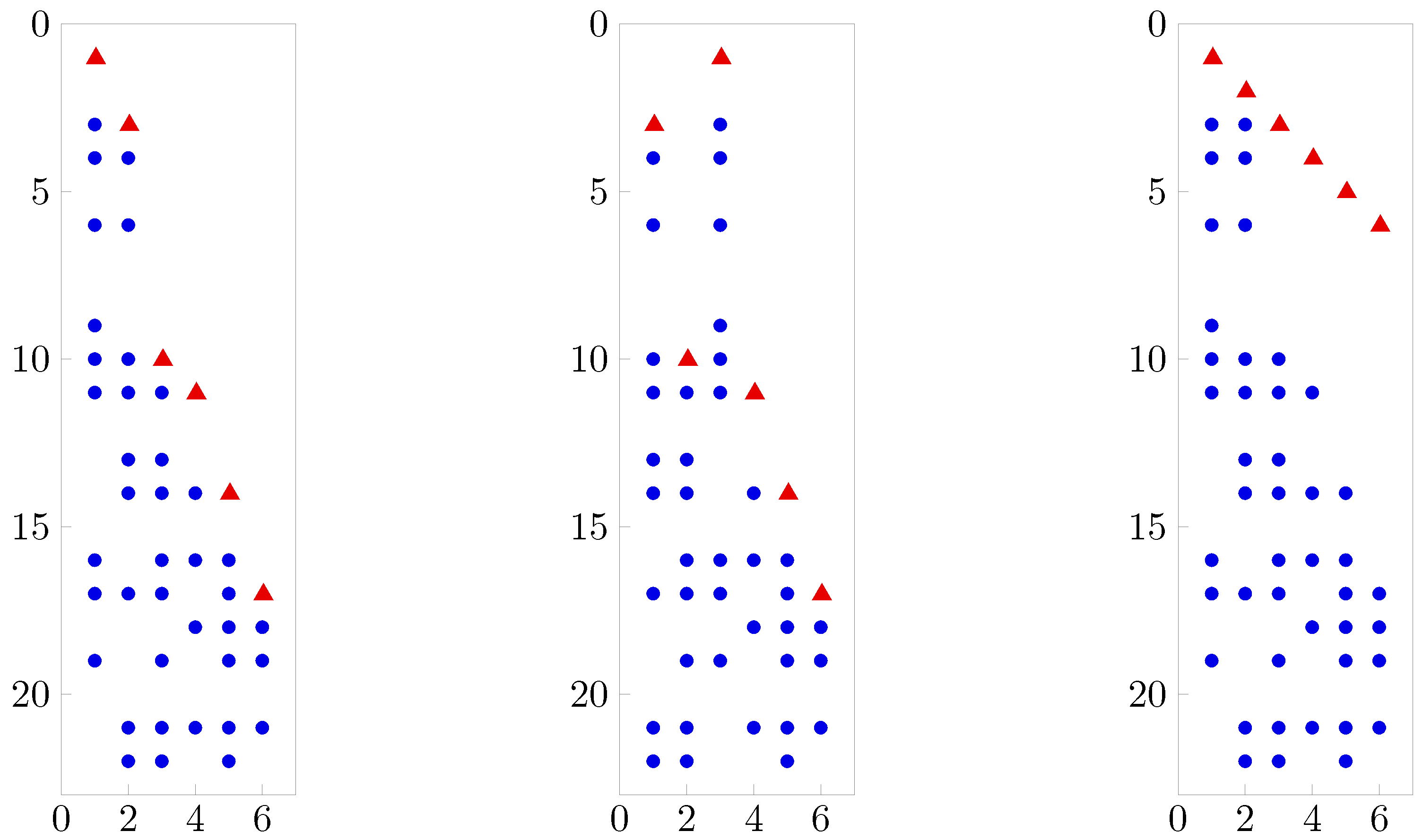
7.1. An Illustrative Simulation Study

For illustration, we perform a simulation study with m = 30 and T = 150 , and consider three different scenarios for the factor loading matrix Λ . In all three scenarios, r true = 5 factors are assumed, but the sparsity matrix δ is quite different. The first setting is a dedicated factor model, where the first six variables load on factor 1, the next six variables load on factor 2, and so forth, and the final six variables load on factor 5. The second scenario is a block factor model, where the first 15 observations load only on factors 1 and 2, while the remaining 15 observations only load on factors 3, 4, and 5, and the covariance matrix has a block-diagonal structure. All factor loadings within a block are non-zero. The third scenario is a dense factor loading matrix without any zero loadings. For all three scenarios, non-zero factor loadings are drawn as λ i j = ( 1 ) b i j ( 1 + 0.1 N 0 , 1 ) , where the exponent b i j is a binary variable with Pr ( b i j = 1 ) = 0.2 . With the exception of the first scenario, no GLT condition is imposed on the simulated loading matrix. In all three scenarios, Σ 0 = I . A total of 21 data sets are sampled under these three scenarios from the basic factor model (1).
The overfitting exploratory factor model (19) with the maximum number of factors H = 14 being equal to the upper bound defined in (13) is fitted to each simulated data set. Regarding rotational invariance, we compare a model where the non-zero columns of the factor loading matrix β k extracted from β H obey an unordered GLT structure with a model where β H is left unconstrained.
Inference is based on the Bayesian approach described in Section 6.1. We consider both a 1PB and a 2PB shrinkage prior on the sparsity matrix δ H , and select the following priors: σ i 2 G 1 2.5 , 1.5 , i = 1 , , 30 , κ G 1 5 , 25 , α G 6 , 2 and γ G 6 , 6 . Using the RJMCMC algorithm of Frühwirth-Schnatter et al. (2023), 3000 posterior draws are generated after a burn-in of 2000 draws.8 As discussed in Section 6.3, the active columns β r are retrieved for each MCMC draw of the loading matrix β H . Under the GLT condition, β r is checked for variance identification using the counting rule CR ( r , 1 ) . For sparse Bayesian factor analysis with unstructured loading matrices, the draws of β r are not screened for variance identification and inference is based on all draws.
For each of the 21 simulated data sets, we evaluate all 12 combinations of data scenarios, structural constraints (GLT versus unconstrained) and priors on the sparsity matrix (1PB versus 2PB) through Monte Carlo estimates of the following statistics: to assess the performance in estimating the true number r true of factors, we consider the mode r ^ of the posterior distribution p ( r | y ) as a point estimator of r. In addition, we consider the magnitude of the posterior ordinate p ( r ^ = r true | y ) as a measure of how strongly the posterior distribution concentrates around the true value. The closer this value is to 1, the smaller is the uncertainty in estimating r. To assess the accuracy in estimating the true covariance matrix Ω 0 = Λ Λ + Σ 0 of the data via the posterior draws of Ω r = β r β r + Σ r , we consider the mean squared error (MSE) defined by
MSE Ω = i i E ( Ω r , i Ω 0 , i 2 | y ) / ( m ( m + 1 ) / 2 ) ,
which accounts both for variance and bias. Table 1 reports, for all 12 combinations, the median, the 5% and the 95% quantile of these statistics across all simulated data sets. For GLT structures, the fraction of variance identified draws is also reported and is, in general, pretty high.
Several conclusions can be drawn from Table 1. First, of all, sparse Bayesian factor analysis under the GLT constraint successfully recovers the true number of factors in all three scenarios. For most of the simulated data sets, the posterior ordinate p ( r ^ = r true | y ) is larger than 0.9. Sparse Bayesian factor analysis with unstructured loading matrices is also quite successful in recovering r true , but with less confidence. Both over- and underfitting is observed, and p ( r ^ = r true | y ) is much smaller than under a GLT structure. For both structures, the 2PB prior yields higher posterior ordinates than the 1PB prior.
Recently, Hosszejni and Frühwirth-Schnatter (2022) proved that the counting rule CR ( r , 1 ) can also be applied to verify variance identification of β r for unconstrained loading matrices. As is evident from Table 1, the fraction of variance identified draws is, however, much smaller than under GLT structures. Nevertheless, inference with respect to to the number of factors can be improved also for an unconstrained EFA model by rejecting all draws of β r that do not obey the counting rule CR ( r , 1 ) .

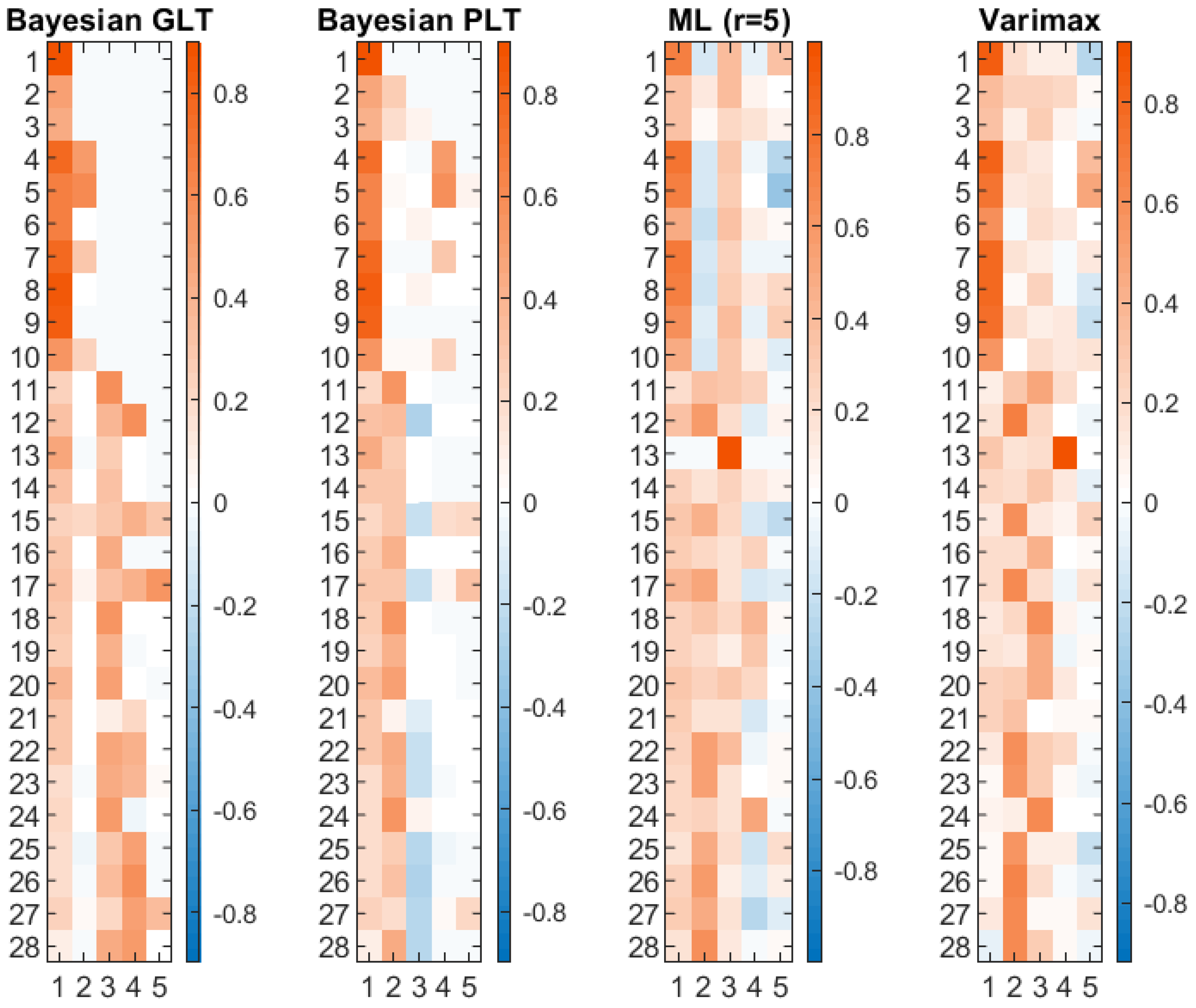
7.2. A Real Data Example

For further illustration, we consider monthly log returns from the New York Stock Exchange (NYSE) for two industry sectors. For each month t = 1 , , T from February 1999 till August 2019 (i.e., T = 247 ), we consider m = 28 firms. The first 10 measurements in y t correspond to all firms in the energy sector, the remaining 18 measurements to all firms in the health care sector.9 We compare sparse Bayesian factor analysis with maximum likelihood estimation and to this aim demean and standardize the data.
Bayesian inference is based on the approach described in Section 6.1. The overfitting exploratory factor model (19) is fitted to this data set under an unordered GLT structure with the maximum number of factors H = 13 being equal to the upper bound defined in (13). MCMC estimation is run for 30,000 iterations after a burn-in of 20,000 using the RJMCMC algorithm of Frühwirth-Schnatter et al. (2023). Prior choices are exactly as in Section 7.1 and we report results for the 2PB prior.
As discussed in Section 6.3, the active columns β r are retrieved for each MCMC draw of the loading matrix β H and checked for variance identification using the counting rule CR ( r , 1 ) . The fraction of variance identified MCMC draws for the 2PB prior is equal to 63%. The number of columns for each variance identified draw β r changes due to the dimension-changing nature of the RJMCMC algorithm and can be considered a posterior draw of the number of active factors r by virtue of Theorem 4. As shown in Table 2, the posterior distribution p ( r | y ) derived in this manner is rather disperse and models from four up to six factors receive considerable posterior probability.
We proceed with the posterior mode estimator of the number of factors and compare various estimators of the factor loading matrix Λ for a basic factor model (1) where r = 5 is assumed. First, we estimate Λ ^ ML using maximum likelihood methods and apply the Varimax procedure to rotate Λ ^ ML into a simple structure Λ ^ VM .10
Second, we derive two Bayesian estimators where we impose, respectively, the PLT and the GLT condition. Under the GLT condition we learn the pivot rows l = ( l 1 , , l 5 ) from the data, while l = ( 1 , , 5 ) under the PLT condition. To identify simple PLT and GLT structures, we perform variable selection beyond the pivot rows and assume the uniform prior τ j B 1 , 1 (instead of 1PB or 2PB shrinkage priors), since the number of factors is known. The prior on the factor loadings and the idiosyncratic variances is the same as before. 10,000 posterior draws are generated by adjusting the algorithm of Frühwirth-Schnatter et al. (2023) to these models. The draws are screened for variance identification using the counting rule CR ( 5 , 1 ) . The average of the variance identified draws immediately yields the Bayesian estimator Λ ^ PLT under the PLT condition.
Under the GLT condition, the sampler operates within an unordered GLT structure with unknown pivot rows. All variance identified posterior draws are identified up to a signed permutation. Full identification is achieved by resolving column and sign switching for each posterior draw. Column switching is resolved by ordering the pivot rows such that l 1 < < l 5 and an ordered GLT structure is imposed on Λ by reordering the columns accordingly. Among these ordered GLT posterior draws of Λ , the combination of pivot rows l ^ = ( 1 , 4 , 11 , 12 , 15 ) is visited most often. All ordered GLT draws where the pivot rows coincide with l ^ are averaged to derive the Bayesian estimator Λ ^ GLT of the GLT factor loading matrix Λ . Beforehand, sign switching in the posterior draws is resolved by imposing the constraint Λ 11 > 0 , Λ 42 > 0 , Λ 11 , 3 > 0 , Λ 12 , 4 > 0 and Λ 15 , 5 > 0 on Λ .
All four estimators are depicted in Figure 2. Note that the measurements are grouped by industry. The pivot rows learned under GLT from the data clearly show that this ordering is in conflict with the PLT assumption. The varimax estimator Λ ^ VM , as well as both Bayesian estimators Λ ^ PLT and Λ ^ GLT , exhibit a simple structure, and sparsity is more pronounced for the two Bayesian estimators due to variable selection on the factor loadings.
Figure 2. Comparing estimators of the loading matrix Λ for the NYSE data (1–10, firms in the energy sector; 11–28, firms in the health care sector) for a basic factor model with r = 5 factors. Heatmaps from left to right: Bayesian estimator Λ ^ GLT of the GLT representation of the loading matrix; Bayesian estimator Λ ^ PLT obtained by imposing a PLT condition; ML estimator Λ ^ ML and the corresponding Varimax rotation Λ ^ VM . Red, white, and blue colors denote positive, zero, and negative values, respectively.
Econometrics 11 00026 g002
In our opinion, the Bayesian GLT estimator Λ ^ GLT allows a clearer interpretation of the four factors than the other estimators. In particular, forcing a PLT assumption leads to a less clear interpretation of the factors. The first factor is a market factor that loads on all 28 firms. The second factor captures additional correlations among the 10 firms in the energy sector, as well as cross-sectional correlations with specific firms in the health care sector. Three additional factors are present that are specific to firms in the health care sector, with factor three loading on nearly all firms in this sector.

8. Concluding Remarks

We have given a full and comprehensive mathematical treatment to generalized lower triangular (GLT) structures, an identification strategy that relaxes the popular positive lower triangular (PLT) assumption for factor loadings matrices. We have proven that GLT retains PLT’s good properties: uniqueness and rotational invariance. At the same time, and unlike PLT, a GLT structure exists for any factor loadings matrix; i.e., it is not a restrictive assumption. Furthermore, we have shown that verifying variance identification under GLT structures is simple and is based purely on the zero-nonzero pattern of the factor loadings matrix. Additionally, we have embedded the GLT model class into exploratory factor analysis with unknown factor dimension and discussed how easily spurious factors and irrelevant variables are recognized in that setup. At the end, we demonstrated our framework in a simulation study and for real data.

Author Contributions

Conceptualization, S.F.-S., D.H. and H.F.L.; methodology, S.F.-S., D.H. and H.F.L.; software, S.F.-S. and D.H.; formal analysis, S.F.-S. and D.H.; investigation, S.F.-S. and D.H.; data curation, S.F.-S. and D.H.; writing—original draft preparation, S.F.-S. and D.H.; writing—review and editing, S.F.-S., D.H. and H.F.L. All authors have read and agreed to the published version of the manuscript.

Funding

Hedibert Freitas Lopes receives support from FAPESP Grant 2018/04654-9.

Data Availability Statement

Restrictions apply to the availability of these data. Data were obtained from Bloomberg and are available from the authors if Bloomberg gives permission.

Conflicts of Interest

The authors declare no conflict of interest.

Appendix A

Proof of Theorem 1.
First, note that G , the result of the procedure described in part (b), exists: there exists a set of r linearly independent rows in β due to its rank r, and therefore the described procedure always succeeds at finding row indices ( l 1 , , l r ) . We show that Λ = β G is an ordered GLT matrix with pivot rows ( l 1 , , l r ) and positive leading elements. This will prove both part (a), which describes that a rotation such as G exists, and part (b), which describes how said G is constructed.
Let the QR-decomposition of β ˜ be β ˜ = G Λ ˜ , where Λ ˜ is the r × r lower triangular submatrix of Λ that consists of, clearly, the l 1 th, …, l r th rows of Λ . We choose G such that Λ ˜ has positive diagonal elements; we can do so according to Golub and Van Loan (2013), and this way G is also unique. We proceed column-by-column in Λ , starting with the first column. Note that Λ l 1 , 1 = Λ ˜ 1 , 1 is positive, therefore l 1 is a candidate for a pivot row. Next, assume that l 1 is not a pivot row because Λ , 1 has a nonzero entry Λ i , 1 for i < l 1 . This implies that β i , contains a nonzero entry, which contradicts how l 1 is found by the procedure. Therefore, l 1 is the pivot row for the first column.
Now, we examine the second column of Λ . Note that Λ l 2 , 2 = Λ ˜ 2 , 2 is positive, so l 2 is a candidate for a pivot row. Also note that Λ l 1 , 2 is zero because it is the second element of Λ ˜ 1 , . Next, assume that l 2 is not a pivot row because Λ , 2 has a nonzero entry Λ i , 2 for i < l 2 . This implies that Λ i , is linearly independent from Λ l 1 , , which implies that β i , is linearly independent from β l 1 , , which contradicts how l 2 is found by the procedure. Therefore, l 2 > l 1 is the pivot row for the second column.
We proceed in this manner, applying the observations for the second column to the third and later columns, until we find that l 1 < l 2 < < l r are the pivot rows of Λ and Λ is ordered GLT. This concludes the proof. □
Lemma A1.
The counting rule C R ( r , s ) has the following properties:
(a) 
C R ( r , s ) holds for δ if C R ( q , s ) holds for every submatrix of q { 1 , , r } columns of δ;
(b) 
If C R ( r , s ) holds for δ and arbitrary s ˜ s rows are deleted from δ, then the remaining matrix satisfies C R ( r , s s ˜ ) ;
(c) 
If C R ( r , s ) holds for δ and some or all zero rows are removed from δ, then C R ( r , s ) also holds for the remaining matrix.
The proof is straightforward.
Proof of Theorem 2.
Any matrix β Θ δ has the same non-zero rows as δ . Hence, if CR ( r , s ) does not hold for δ , then it also does not hold for any β Θ δ . According to Theorem 3.4. by Sato (1992) with their rotation G being the identity, this implies that RD ( r , s ) is violated for all β Θ δ . This proves part (a).
We prove part (b) by induction. If CR ( 1 , s ) holds for a m × 1 sparsity vector δ , then at least m 1 2 + s elements of δ are different from 0. It trivially follows that all β Θ δ have same number of non-zero elements. After deleting s elements, two subvectors with at least one non-zero element can be formed and RD ( 1 , s ) is satisfied for β . For any r 2 , assume that part (b) of Theorem 2 holds for r 1 and that the counting rule CR ( r , s ) holds for an m × r ordered GLT sparsity matrix δ . A suitable permutation of the rows of δ yields:
Π r δ = δ c 0 δ b δ A ,
where δ A is a GLT sparsity matrix with r 1 columns, δ b and δ c are column vectors, and δ c contains d 1 1 non-zero elements and no zero elements. According to Lemma A1 δ A satisfies CR ( r 1 , s ) and the first column ( ( δ c ) , ( δ b ) ) satisfies CR ( 1 , s ) . Consequently, δ b contains at least 2 + s d 1 non-zero elements. Let Λ Θ δ be an ordered GLT matrix. If the same s rows are deleted from Π r δ and Π r Λ , we obtain the following matrices:
δ ˜ = δ ˜ c 0 δ ˜ b δ ˜ A , Λ ˜ = Λ ˜ c 0 Λ ˜ b Λ ˜ A ,
where 0 s 1 min ( d 1 , s ) non-zero elements are deleted from the vector δ c and d 1 s 1 non-zero elements remain in the vectors δ ˜ c and Λ ˜ c , while the vectors δ ˜ b and Λ ˜ b contain d 2 max ( 0 , 2 + s 1 d 1 ) non-zero elements. Since we removed s s 1 rows from δ A , according to Lemma A1(b), the sparsity matrix δ ˜ A satisfies CR ( r 1 , s 1 ) and, hence, Λ ˜ A obeys RD ( r 1 , s 1 ) except for a set of measure 0. We proceed with those matrices Λ ˜ A where RD ( r 1 , s 1 ) holds. If further s 1 rows are deleted from Λ ˜ A , then a matrix results which contains two sub matrices A 1 and A 2 of rank r 1 . Let the s 1 × ( r 1 ) matrix B contain the rows that were deleted from of Λ ˜ A . If the same rows are deleted from Λ ˜ b , then the vector b containing the deleted elements has at least max(0, 2 − (d1s1)) non-zero elements. Next, we consider three cases. First, if d1s1 ≥ 2, then we use two of the d1s1 non-zero elements of δ ˜ c to define the following submatrices of Λ:
δ ˜ i 1 c 0 × A 1 , δ ˜ i 2 c 0 × A 2 .
Both matrices obviously have rank r. Second, if d1s1 = 1, then we use the only non-zero element of δ ˜ c and one of the non-zero elements of b, denoted by b i 2 , and the corresponding row B i 2 , of B to define the following submatrices of Λ :
δ ˜ i 1 c 0 × A 1 , b i 2 B i 2 , × A 2 .
The first matrix obviously has rank r . The rank of the second matrix is at least equal to rk ( A 2 ) = r 1 . The row vector B i 2 , contains 0 d 3 r 1 non-zero elements, which take arbitrary values in R . Hence, the set of matrices where the row ( b i 2 B i 2 , ) is linearly dependent on the other rows and rank deficiency occurs has measure zero. Finally, if d 1 s 1 = 0 , then we use two of the at least two non-zero elements in b, denoted by b i 1 and b i 2 and the corresponding rows B i 1 , and B i 2 , of B to define the following submatrices of Λ:
b i 1 B i 1 , × A 1 , b i 2 B i 2 , × A 2 .
Using the same argument as above, both matrices are of rank r , except for a set of measure 0. This proves that RD ( r , s ) holds for all GLT matrices Λ Θ δ , except for a set of measure 0. The counting rule CR ( r , s ) is invariant to signed permutations of δ . Therefore, if CR ( r , s ) implies RD ( r , s ) for an ordered GLT matrix Λ Θ δ , then this holds for all signed permutations β = Λ P ± P ρ of Λ . This completes the proof of part (b), since the set where RD ( r , s ) does not hold is a finite union of sets of measure 0. □
Proof of Corollary 3.
The conditions in Corollary 3 follow immediately from Theorem 2. The ( j , l ) th elements of the matrix on the left hand of (16) is given by d j + i = 1 m δ i j ( 1 δ i l ) , where d j = i = 1 m δ i j is the total number of non-zero indicators in column j. The diagonal elements ( j = l ) are equal to d j (since δ i j ( 1 δ i j ) = 0 ) and check if each column contains at least 2 + s non-zero indicators. The off-diagonal elements ( j l ) count the number of nonzero rows in columns j and l. Hence, the matrix on the right hand of (16) has diagonal elements equal to 2 + s and off-diagonal elements equal to 4 + s . The column vector δ in (17) is equal to the number of non-zero indicators in each row. Hence, (17) verifies if the total number of nonzero rows of δ is at least equal to 2 r + s . Finally, (18) verifies if each submatrix of r 1 columns has at least 2 r 1 nonzero rows. The jth column of the matrix δ in (18) is the number of non-zero indicators in each row of the submatrix δ j excluding the jth column. The matrix I ( δ > 0 ) indicates nonzero rows in δ j and the jth element of the row vector 1 1 × m · I ( δ > 0 ) counts the number of nonzero rows in δ j . □
Proof of Theorem 4.
We start by proving further properties of the spurious factor matrix M s in representation (26) beyond the characterization given in Tumura and Sato (1980, Theorem 1). More specifically, we show that the spurious cross-covariance matrix M s M s = D s is equal to a diagonal matrix of rank s, with s nonzero entries d n 1 , , d n s in rows n 1 , , n s . From rk ( β k T k ) = min ( rk ( β k ) , rk ( T k ) ) = r + s , we obtain that M s has full column rank rk ( M s ) = s . Therefore, rk ( D s ) = rk ( M s ) = s and only s diagonal elements d n 1 , , d n s of D s in rows n 1 , , n s are different from 0. It follows that M s has exactly the same s nonzero rows n 1 , , n s as D s : using for each row M i , · of M s that M i , · M i , · = M i , · 2 2 = d i , it follows for any i { n 1 , , n s } that M i , · 2 2 = 0 and, therefore, M i , · = 0 , whereas the remaining rows with i { n 1 , , n s } are nonzero, since M i , · 2 2 > 0 . The submatrix M 0 of nonzero rows in M s satisfies M 0 M 0 = D 0 2 with D 0 2 = Diag d n 1 , , d n s being a diagonal matrix of rank s. It follows that D 0 1 M s D 0 1 M s = I , hence D 0 1 M s = Q for any arbitrary rotation matrix Q of rank s. Therefore, M 0 = D 0 Q .
These results allow following representation of the β k T k in (26). Let β k , Σ k , M s , Λ , and Σ 0 , be the matrices that result from deleting the rows n 1 , , n s (and for Σ k and Σ 0 also the columns) from the matrices β k , Σ k , M s , Λ , and Σ 0 . Since M s = O , we obtain:
β k T k = Λ O , Σ k = Σ 0 .
Condition R D ( r , 1 + S ) for Λ implies that Λ satisfies condition R D ( r , 1 ) , and the variance decomposition Ω = Λ ( Λ ) + Σ 0 is unique. Hence, β k ( β k ) = Λ ( Λ ) and β k has reduced rank rk ( β k ) = rk ( Λ ) = r . Regarding the s rows β k d and Λ d that were deleted from, respectively, β k and Λ , we obtain
β k d T k = Λ d M 0 , M 0 = D 0 Q ,
where D 0 is a diagonal matrix and Q is an arbitrary rotation matrix, both of rank s. These results are valid regardless of the conditions imposed on β k to resolve rotational invariance (if any). If an unordered GLT condition is imposed, then it can be shown that M 0 is a spurious unordered GLT matrix and T k reduces to a signed permutation. Without loss of generality, we assume that the true loading matrix Λ also takes the form of an unordered GLT structure.
First, we show that under an unordered GLT condition β k takes a similar form as β k T k does in (A4) and (A5), up to a signed permutation. β k has rk ( β k ) = r + s distinct pivot rows. Let n 1 , , n s be the non-zero rows in the spurious loading matrix M s . When these rows are deleted from β k , the resulting matrix β k has reduced rank r which implies that s among the r + s pivot rows of β k are identical to n 1 , , n s . Furthermore, β k contains a m × r submatrix β r that obeys an unordered GLT condition with the remaining r rows serving as pivots. Since both β k and β r have rank r, the remaining m × s submatrix of β k has rank zero, and is equal to a nullmatrix except for a set of measure zero. Hence, a signed permutation matrix P of size r + s can be used to reorder the columns of β k :
β k P = β r O .
If the same signed permutation is applied to β k d , then we obtain:
β k d P = β r d β s ,
where β r d is an s × r matrix. The s × s submatrix β s has an unordered GLT structure with pivot rows n 1 , , n s and is equal to a lower triangular matrix L ˜ of rank s up to column switching, i.e., β s = L ˜ P ˜ ρ .
Next, let us investigate the spurious submatrix M 0 in (A5). Since under an unordered GLT condition, any rotation β k T k generated from β k through (26) also exhibits an unordered GLT structure, it follows from (A4) and (A5) that M 0 is an unordered GLT matrix with pivot rows n 1 , , n s . Therefore, M 0 = L P ρ is equal to a lower triangular matrix L up to column switching. From L L = M 0 M 0 = D 0 2 , it follows that L = D 0 P ± is equal to the diagonal matrix D 0 up to sign switching and, therefore:
M 0 = D 0 P M ,
where P M is a signed permutation of size s. This proves the first claim that under the unordered GLT framework, that the spurious factor matrix of any rotation β k T k generated through (26) can be represented as a spurious unordered GLT matrix M s .
To complete the proof, we show that the rotation matrix T defined by T : = P T k is a signed permutation. T is split it in the following way:
T = T 1 T 3 ( T 3 ) T 2 ,
with square matrices T 1 and T 2 of size r and s. We obtain from (A4) and (A6):
β k T k = β k P P T k = β r T 1 β r T 3 = Λ O .
Since β r has full column rank, we obtain from β r T 3 = O by left multiplication with ( ( β r ) β r ) 1 ( β r ) that T 3 = O . Furthermore, β r T 1 = Λ . Application of Corollary 1 to the unordered GLT matrix β r , which satisfies β r ( β r ) = Λ ( Λ ) , yields β r = Λ P r , where P r is a signed permutation of size r. From β r T 1 = Λ = β r P r , we obtain that T 1 = P r is a signed permutation. Finally, we obtain from (A5), (A7), and (A8):
β k d T k = β k d P T = β r d β s T = β r d P r L ˜ P ˜ ρ T 2 = Λ d D 0 P M .
It follows that L ˜ L ˜ = D 0 2 , and therefore the lower triangular matrix L ˜ is equal to D 0 up to sign switching. Consequently, L ˜ P ˜ ρ T 2 = D 0 P s T 2 = D 0 P M , where P s is a signed permutation of size s. It follows immediately that T 2 = P s P M is also a signed permutation matrix of size s. Therefore, both the rotation matrix T defined in (A9), as well as T k = T P , are signed permutations of size r + s . □

Notes

1
The sign condition on Λ i i is needed to avoid sign switching, since 2 r 1 loading matrices β can be constructed, which differ from Λ by a sign switch in a subset of columns, but yield the same cross-covariance matrix β β = Λ Λ (see also Section 3). Without sign conditions, Λ would not be identified. However, any other sign condition, such as Λ i i < 0 , i = 1 , , r , could be applied.
2
Our use of the term “pivot” is inspired by the concept of pivot columns in a row reduced echelon form (RREF), which is the result of Gauss–Jordan elimination. In particular, if Λ is in RREF, then pivot rows of Λ are the pivot columns of Λ . For more details, see, e.g., Anton and Rorres (2013).
3
The pivot rows l 1 , , l r thus coincide with the pivot columns of the row reduced echelon form (RREF) of β .
4
Their algorithm for the efficient verification of CR ( r , 1 ) is implemented in R and MATLAB. The computer code is publicly available at https://github.com/hdarjus/sparvaride (accessed on 31 October 2023) and, respectively, https://github.com/hdarjus/sparvaride-matlab (accessed on 31 October 2023).
5
Note that the non-spurious columns of β ˜ 3 form an unordered GLT structure, while Λ is GLT.
6
Evidently, zero columns (if any) in a posterior draw of β H can be ignored, since β H β H = β k β k .
7
It should be noted that Dirac-spike-and-slab priors such as (29) are useful in this regard, since they are able to identify the ( m 1 ) s exact zeros in the columns corresponding to spurious factors. Under continuous shrinkage priors *(see, e.g., Bhattacharya and Dunson (2011); Ročková and George (2017)), how to identify and remove spurious factors is not straightforward.
8
This algorithm is designed for inference in EFA models under the GLT condition, but can be easily extended to models with unconstrained loading matrices β H .
9
See Frühwirth-Schnatter et al. (2023) for a case study involving additional industry sectors.
10
These computation were carried out using the function factoran in MATLAB.

References

  1. Anderson, Brian David Outram, Manfred Deistler, Elisabeth Felsenstein, Bernd Funovits, Lukas Koelbl, and Mohsen Zamani. 2016. Multivariate AR systems and mixed frequency data: G-identifiability and estimation. Econometric Theory 32: 793–826. [Google Scholar] [CrossRef]
  2. Anderson, Theodore Wilbur. 2003. An Introduction to Multivariate Statistical Analysis, 3rd ed. Chichester: Wiley. [Google Scholar]
  3. Anderson, Theodore Wilbur, and Herman Rubin. 1956. Statistical inference in factor analysis. Paper presented at Third Berkeley Symposium on Mathematical Statistics and Probability, Berkeley, CA, USA, December 26–31; Volume V, pp. 111–50. [Google Scholar]
  4. Anton, Howard, and Chris Rorres. 2013. Elementary Linear Algebra, 11th ed. Hoboken: Wiley Global Education. [Google Scholar]
  5. Aßmann, Christian, Jens Boysen-Hogrefe, and Markus Pape. 2016. Bayesian analysis of static and dynamic factor models: An ex-post approach toward the rotation problem. Journal of Econometrics 192: 190–206. [Google Scholar] [CrossRef]
  6. Bai, Jushan, and Serena Ng. 2002. Determining the number of factors in approximate factor models. Econometrica 70: 191–221. [Google Scholar] [CrossRef]
  7. Bai, Jushan, and Serena Ng. 2013. Principal components estimation and identification of static factors. Journal of Econometrics 176: 18–29. [Google Scholar] [CrossRef]
  8. Bartholomew, David John. 1987. Latent Variable Models and Factor Analysis. London: Charles Griffin. [Google Scholar]
  9. Bekker, Paul A. 1989. Identification in restricted factor models and the evaluation of rank conditions. Journal of Econometrics 41: 5–16. [Google Scholar] [CrossRef]
  10. Bhattacharya, Anirban, and David Brian Dunson. 2011. Sparse Bayesian infinite factor models. Biometrika 98: 291–306. [Google Scholar] [CrossRef]
  11. Boivin, Jean, and Serena Ng. 2006. Are more data always better for factor analysis? Journal of Econometrics 132: 169–94. [Google Scholar] [CrossRef]
  12. Carvalho, Carlos M., Jeffrey Chang, Joseph E. Lucas, Joseph R. Nevins, Quanli Wang, and Mike West. 2008. High-dimensional sparse factor modeling: Applications in gene expression genomics. Journal of the American Statistical Association 103: 1438–56. [Google Scholar] [CrossRef]
  13. Chan, Joshua, Roberto Leon-Gonzalez, and Rodney W. Strachan. 2018. Invariant inference and efficient computation in the static factor model. Journal of the American Statistical Association 113: 819–28. [Google Scholar] [CrossRef]
  14. Conti, Gabriella, Sylvia Frühwirth-Schnatter, James Joseph Heckman, and Rémi Piatek. 2014. Bayesian exploratory factor analysis. Journal of Econometrics 183: 31–57. [Google Scholar] [CrossRef]
  15. Fan, Jianqing, Yingying Fan, and Jinchi Lv. 2008. High dimensional covariance matrix estimation using a factor model. Journal of Econometrics 147: 186–97. [Google Scholar] [CrossRef]
  16. Forni, Mario, Domenico Giannone, Marco Lippi, and Lucrezia Reichlin. 2009. Opening the black box: Structural factor models with large cross sections. Econometric Theory 25: 1319–47. [Google Scholar] [CrossRef]
  17. Frühwirth-Schnatter, Sylvia. 2023. Generalized cumulative shrinkage process priors with applications to sparse Bayesian factor analysis. Philosophical Transactions of the Royal Society A. forthcoming. [Google Scholar] [CrossRef] [PubMed]
  18. Frühwirth-Schnatter, Sylvia, and Hedibert F. Lopes. 2018. Sparse Bayesian factor analysis when the number of factors is unknown. arXiv arXiv:1804.04231. [Google Scholar]
  19. Frühwirth-Schnatter, Sylvia, Darjus Hosszejni, and Hedibert Freitas Lopes. 2023. Sparse Bayesian factor analysis when the number of factors is unknown. arXiv arXiv:2301.06459. [Google Scholar]
  20. Geweke, John Frederick, and Guofu Zhou. 1996. Measuring the pricing error of the arbitrage pricing theory. Review of Financial Studies 9: 557–87. [Google Scholar] [CrossRef]
  21. Geweke, John Frederick, and Kenneth James Singleton. 1980. Interpreting the likelihood ratio statistic in factor models when sample size is small. Journal of the American Statistical Association 75: 133–37. [Google Scholar] [CrossRef]
  22. Golub, Gene H., and Charles F. Van Loan. 2013. Matrix Computations, 4th ed. Baltimore: Johns Hopkins University Press. [Google Scholar]
  23. Hayashi, Kentaro, and George A. Marcoulides. 2006. Examining identification issues in factor analysis. Structural Equation Modeling 13: 631–45. [Google Scholar] [CrossRef]
  24. Hosszejni, Darjus, and Sylvia Frühwirth-Schnatter. 2022. Cover it up! Bipartite graphs uncover identifiability in sparse factor analysis. arXiv arXiv:2211.00671. [Google Scholar]
  25. Jöreskog, Karl Gustav. 1969. A general approach to confirmatory maximum likelihood factor analysis. Psychometrika 34: 183–202. [Google Scholar]
  26. Kastner, Gregor. 2019. Sparse Bayesian time-varying covariance estimation in many dimensions. Journal of Econometrics 210: 98–115. [Google Scholar] [CrossRef]
  27. Kaufmann, Sylvia, and Christian Schumacher. 2017. Identifying relevant and irrelevant variables in sparse factor models. Journal of Applied Econometrics 32: 1123–44. [Google Scholar] [CrossRef]
  28. Kaufmann, Sylvia, and Christian Schumacher. 2019. Bayesian estimation of sparse dynamic factor models with order-independent and ex-post identification. Journal of Econometrics 210: 116–34. [Google Scholar] [CrossRef]
  29. Koopmans, Tjalling Charles, and Olav Reiersøl. 1950. The identification of structural characteristics. The Annals of Mathematical Statistics 21: 165–81. [Google Scholar] [CrossRef]
  30. Ledoit, Olivier, and Michael Wolf. 2020. The power of (non-)linear shrinking: A review and guide to covariance matrix estimation. Journal of Financial Econometrics 20: 187–218. [Google Scholar] [CrossRef]
  31. Lee, Sik-Yum, and Xin-Yuan Song. 2002. Bayesian selection on the number of factors in a factor analysis model. Behaviormetrika 29: 23–39. [Google Scholar] [CrossRef]
  32. Legramanti, Sirio, Daniele Durante, and David B. Dunson. 2020. Bayesian cumulative shrinkage for infinite factorizations. Biometrika 107: 745–52. [Google Scholar] [CrossRef]
  33. Lopes, Hedibert Freitas, and Mike West. 2004. Bayesian model assessment in factor analysis. Statistica Sinica 14: 41–67. [Google Scholar]
  34. Magnus, Jan R., and Heinz Neudecker. 2019. Matrix Differential Calculus with Applications in Statistics and Econometrics. Hoboken: John Wiley & Sons. [Google Scholar]
  35. Neudecker, Heinz 1990. On the identification of restricted factor loading matrices: An alternative condition. Journal of Mathematical Psychology 34: 237–41. [CrossRef]
  36. Ohn, Ilsang, and Yongdai Kim. 2022. Posterior consistency of factor dimensionality in high-dimensional sparse factor models. Bayesian Analysis 17: 491–514. [Google Scholar] [CrossRef]
  37. Owen, Art B., and Jingshu Wang. 2016. Bi-cross-validation for factor analysis. Statistical Science 31: 119–39. [Google Scholar] [CrossRef]
  38. Reiersøl, Olav. 1950. On the identifiability of parameters in Thurstone’s multiple factor analysis. Psychometrika 15: 121–49. [Google Scholar] [CrossRef] [PubMed]
  39. Ročková, Veronika, and Edward I. George. 2017. Fast Bayesian factor analysis via automatic rotation to sparsity. Journal of the American Statistical Association 111: 1608–22. [Google Scholar] [CrossRef]
  40. Sato, Manabu. 1992. A study of an identification problem and substitute use of principal component analysis in factor analysis. Hiroshima Mathematical Journal 22: 479–524. [Google Scholar] [CrossRef]
  41. Teh, Yee Whye, Dilan Görür, and Zoubin Ghahramani. 2007. Stick-breaking construction for the Indian buffet process. Paper presented at Eleventh International Conference on Artificial Intelligence and Statistics, Proceedings of Machine Learning Research (PMLR), San Juan, Puerto Rico, March 21–24; Edited by Marina Meila and Xiaotong Shen. vol. 2, pp. 556–63. [Google Scholar]
  42. Thurstone, Louis Leon. 1935. The Vectors of Mind. Chicago: University of Chicago. [Google Scholar]
  43. Thurstone, Louis Leon. 1947. Multiple Factor Analysis. Chicago: University of Chicago. [Google Scholar]
  44. Tumura, Yosiro, and Manabu Sato. 1980. On the identification in factor analysis. TRU Mathematics 16: 121–31. [Google Scholar]
  45. West, Mike. 2003. Bayesian factor regression models in the “large p, small n” paradigm. In Bayesian Statistics 7. Edited by José Miguel Bernardo, María Jesús Bayarri, James Orvis Berger, Alexander Philip Dawid, David Heckerman, Adrian Frederick Melhuish Smith and Mike West. Oxford: Oxford University Press, pp. 733–42. [Google Scholar]
  46. Williams, Benjamin. 2020. Identification of the linear factor model. Econometric Reviews 39: 92–109. [Google Scholar] [CrossRef]
  47. Zhao, Shiwen, Chuan Gao, Sayan Mukherjee, and Barbara E. Engelhardt. 2016. Bayesian group factor analysis with structured sparsity. Journal of Machine Learning Research 17: 1–47. [Google Scholar]
Figure 1. (Left): simple ordered GLT matrix with six factors and pivot rows ( l 1 , , l 6 ) = ( 1 , 3 , 10 , 11 , 14 , 17 ) . (Center): one of the 2 6 · 6 ! corresponding simple unordered GLT matrices with pivot rows ( l 1 , , l 6 ) = ( 3 , 10 , 1 , 11 , 14 , 17 ) . (Right): a corresponding simple PLT matrix, i.e., enforced non-zeros on the main diagonal, with pivot rows ( l 1 , , l 6 ) = ( 1 , 2 , 3 , 4 , 5 , 6 ) . Pivot rows are marked by triangles, unconstrained loadings are marked by circles, and zero loadings are left blank.
Econometrics 11 00026 g001
Table 1. Sparse Bayesian factor analysis under GLT and unconstrained structures (EFA) under a 1PB prior ( α G 6 , 2 ) and a 2PB prior ( α G 6 , 2 , γ G 6 , 6 ). The true number of factors is equal to 5. GLT and EFA-V use only the variance identified draws ( M V is the percentage of variance identified draws), EFA uses all posterior draws.
M V r ^ p ( r ^ = r true | y ) MSE Ω
ScenarioPriorMed (QR)Med (QR)Med (QR)Med (QR)
DedicGLT1PB97.0 (91.5, 98.3)5 (5, 5)0.90 (0.94, 0.99)0.018 (0.014, 0.030)
2PB97.6 (87.7, 98.9)5 (5, 5)0.99 (0.83, 1.00)0.019 (0.016, 0.027)
EFA1PB-5 (5, 6)0.66 (0.09, 0.79)0.020 (0.015, 0.026)
2PB-5 (5, 6)0.69 (0.36, 0.80)0.019 (0.014, 0.024)
EFA-V1PB80.3 (49.8, 87.0)5 (5, 6)0.81 (0.17, 0.91)0.020 (0.015, 0.026)
2PB82.6 (63.4, 87.9)5 (5, 6)0.84 (0.53, 0.92)0.019 (0.014, 0.024)
BlockGLT1PB96.5 (39.4, 98.9)5 (5, 5)0.99 (0.28, 0.99)0.12 (0.08, 0.18)
2PB98.7 (61.9, 99.4)5 (5, 5)0.99 (0.54, 1.00)0.10 (0.08, 0.14)
EFA1PB-5 (4, 5)0.78 (0.22, 0.88)0.14 (0.11, 0.20)
2PB-5 (4, 5)0.79 (0.08, 0.89)0.12 (0.08, 0.24)
EFA-V1PB87.0 (55.0, 91.5)5 (4, 5)0.89 (0.09, 0.96)0.14 (0.11, 0.20)
2PB85.9 (28.3, 90.4)5 (4, 5)0.92 (0.03, 0.97)0.12 (0.08, 0.24)
DenseGLT1PB95.7 (84.6, 98.6)5 (5, 5)0.98 (0.92, 0.99)0.67 (0.44, 1.12)
2PB99.4 (90.8, 99.8)5 (5, 5)0.99 (0.93, 1.00)0.68 (0.51, 1.18)
EFA1PB-5 (5, 6)0.76 (0.43, 0.85)0.54 (0.39, 0.76)
2PB-5 (5, 5)0.80 (0.66, 0.91)0.59 (0.43, 0.90)
EFA-V1PB84.4 (76.0, 90.2)5 (5, 6)0.89 (0.57, 0.95)0.54 (0.39, 0.76)
2PB89.7 (80.4, 93.9)5 (5, 5)0.93 (0.77, 0.98)0.59 (0.43, 0.90)
Med is the median and QR are the 5% and the 95% quantile of the various statistics over the 21 simulated data sets.
Table 2. Posterior distribution p ( r | y ) of the number of factors based on all variance identified posterior draws.
r0–3456789–13
p ( r | y ) 00.280.450.250.020.0010
Disclaimer/Publisher’s Note: The statements, opinions and data contained in all publications are solely those of the individual author(s) and contributor(s) and not of MDPI and/or the editor(s). MDPI and/or the editor(s) disclaim responsibility for any injury to people or property resulting from any ideas, methods, instructions or products referred to in the content.

