On the Proper Computation of the Hausman Test Statistic in Standard Linear Panel Data Models: Some Clarifications and New Results

Abstract

We provide new analytical results for the implementation of the Hausman specification test statistic in a standard panel data model, comparing the version based on the estimators computed from the untransformed random effects model specification under Feasible Generalized Least Squares and the one computed from the quasi-demeaned model estimated by Ordinary Least Squares. We show that the quasi-demeaned model cannot provide a reliable magnitude when implementing the Hausman test in a finite sample setting, although it is the most common approach used to produce the test statistic in econometric software. The difference between the Hausman statistics computed under the two methods can be substantial and even lead to opposite conclusions for the test of orthogonality between the regressors and the individual-specific effects. Furthermore, this difference remains important even with large cross-sectional dimensions as it mainly depends on the within-between structure of the regressors and on the presence of a significant correlation between the individual effects and the covariates in the data. We propose to supplement the test outcomes that are provided in the main econometric software packages with some metrics to address the issue at hand.

1. Introduction

As is well known, the implementation of the Hausman specification test (Hausman 1978) might be affected, in practice and in a finite sample setting, by a non-positive definiteness or (in-) definiteness problem for the variance-covariance matrix corresponding to the difference between the efficient estimator and the consistent estimator1. This, in turn, can potentially lead to a negative value of the test statistic, which makes it unreliable for interpreting the test outcome. This problem is usually mentioned in the context of models using instrumental variables (IV) (Baum et al. 2003, pp. 19–22; Staiger and Stock 1997, pp. 567–68) where the Hausman test is performed to assess the endogeneity of the regressors, given a set of instruments. In this case, one solution to ensure a symmetric positive definite (hereafter, SPD) covariance matrix is to use a common and identical estimator for the variance of the (idiosyncratic) error term when confronting the Ordinary Least Squares (OLS) and the IV estimators (Hayashi 2000, pp. 220–33; Baum et al. 2003, pp. 19–22).

Yet, although the issue has been pointed out as a warning by Hausman himself when he addressed the case of a static balanced, panel data model in his seminal presentation of the test (Hausman 1978, footnote 25, p. 1267), it has not been, to the best of our knowledge, further formally examined in this specific framework2. This is surprising, as one of the most widespread applications of the Hausman test is for assessing the relevance of the random (RE) versus fixed effects (FE) specification in a panel data model. From our point of view, this application, however, deserves attention in its own right, and this article aims at filling this gap. Specifically, our contributions are twofold.

We first provide new and detailed analytical results for the implementation of the Hausman test in the case of a static and balanced panel data model with individual effects. In particular, we show that the test statistic is unreliable in a finite sample if the variance of the RE estimator is computed on the basis of the estimation of the quasi-demeaned model (we denote it in what follows QDM)3 rather than the conventional and direct implementation of the Feasible Generalized Least Squares (FGLS) on the RE panel data model. This result directly follows from the way in which standard errors are computed under the QDM approach and which can lead to a positive definiteness problem for the covariance matrix in the Hausman test statistic formula. To establish the unreliability, we perform a systematic analysis of the difference between the Hausman statistics computed under the two approaches as well as of the behavior of the statistic that uses the estimates based on the QDM regression framework. In particular, we show that the latter mainly depends on the within-between structure of the regressors and on the presence of a significant correlation between the individual effects and the covariates in the data4.

Second, based on a review of the main existing econometric software programs that deal with panel data models, we show that the vast majority of the related packages in those programs implement, by default, the Hausman test using the unreliable statistic. This leads us to assess different ways to supplement the test outcomes provided by those programs and/or to circumvent the reliability problem potentially raised by the use of the statistic involved.

The outline of the paper is as follows. First, in Section 2, we show how the two versions of the Hausman test statistics can produce diverging results for some well-known textbook examples in the context of panel data models. Then, in Section 3, we formalize the implications of the two approaches for the Hausman statistic and derive new analytical results regarding the comparison of the two versions of the statistic that follows from each of the two approaches. We also revisit textbook examples and provide some simulation results in the one-regressor case. Finally, in Section 4, we detail how the Hausman test is implemented in a variety of econometric software programs dealing with panel data models and discuss, on the basis of this review, some possible ways to implement this test in a reliable and robust manner with this software. The last section concludes.

2. Motivation

In this section, we illustrate the extent to which significant differences in the values of the Hausman test statistic may arise depending on the approach adopted to estimate the panel data model parameters and, more particularly, those pertaining to the variance components under the random effects (RE) specification.

2.1. Notation

All the case studies considered below are for a standard, linear, static, and balanced panel data model with individual effects (also called the one-way error component-panel data-model). Accordingly, we consider the following relationship:

$$y_{it}=\alpha +X_{it}^{\prime }·\beta +u_{it}$$

(1)

where $i=1,\dots ,N$ denotes the cross-section dimension; $t=1,\dots ,T$ the time-series dimension; $y_{it}$ the $it$-th observation of the dependent variable; $X_{it}$ a column vector of the $it$-th observation on K explanatory variables; $\alpha$ an unknown scalar and $\beta$ a $\left(K\times 1\right)$ vector of unknown parameters, both to be estimated5. The error term $u_{it}$ is assumed to take the following composite form:

$$u_{it}={\alpha }_i^{*}+{\epsilon }_{it}$$

(2)

where ${\alpha }_i^{*}$ denotes the (unobservable) individual-specific (or individual) effect-also called the individual component of $u_{it}$ and ${\epsilon }_{it}$ denotes the idiosyncratic component of $u_{it}$. Furthermore, we assume that ${\alpha }_i^{*}$ and ${\epsilon }_{it}$ are independent of each other and that ${\alpha }_i^{*}\sim IID(0,{\sigma }_{\alpha }^2)$ and ${\epsilon }_{it}\sim IID(0,{\sigma }_{\epsilon }^2)$. It is also assumed that $E[X_{is}·{\epsilon }_{it}]=0$ for all $s=1,\dots ,T$.

As is well known, two alternative specifications are usually considered regarding the correlation between the individual effect, ${\alpha }_i^{*}$ and the regressors contained in $X_{it}$. On the one hand, the random-effects (RE) model assumes that this correlation is zero, ensuring that $X_{it}$ is strictly exogenous for $u_{it}$ in (1). On the other hand, the ‘fixed effects’ model allows for a non-zero correlation between the individual effect and the regressors. The Within transformation is then used to obtain an unbiased estimate for $\beta$.

The Hausman specification test (Hausman 1978) is widely used for testing the no-correlation assumption underlying the RE specification. In our setting, the test is based on the asymptotic properties of the RE and Within (or fixed-effects) estimators of $\beta$. Both estimators are consistent under the null hypothesis (of no correlation) while, under the alternative, only the Within estimator is consistent as the RE estimator is (asymptotically) biased. Accordingly, the test statistic is built on a distance measure between the Within and RE estimators. In its implementable version, the statistic writes as:

$$H{M}_O^j\equiv {({\widehat{\beta }}_W-{\widehat{\beta }}_{RE})}^{\prime }·{\left\{\mathbf{v}\widehat{\mathbf{a}}\mathbf{r}\left[{\widehat{\beta }}_W\right]-\mathbf{v}\widehat{\mathbf{a}}{\mathbf{r}}_j\left[{\widehat{\beta }}_{RE}\right]\right\}}^{-1}·({\widehat{\beta }}_W-{\widehat{\beta }}_{RE})$$

where ${\widehat{\beta }}_W$ and $\mathbf{v}\widehat{\mathbf{a}}\mathbf{r}\left[{\widehat{\beta }}_W\right]$ denote the Within (or fixed effects) estimator of $\beta$ and a consistent estimator of its asymptotic covariance matrix, respectively; ${\widehat{\beta }}_{RE}$ and $\mathbf{v}\widehat{\mathbf{a}}{\mathbf{r}}_j\left[{\widehat{\beta }}_{RE}\right]$ denote the RE estimator of $\beta$ and a consistent estimator of its asymptotic covariance matrix, respectively. The index $j=1,2$ indicates that two approaches can be considered to obtain a consistent estimator of the asymptotic covariance matrix, leading to two versions of the test statistic (see Section 3.3).

2.2. Motivating Examples

We reproduce some outcomes of panel model estimations for well-known case study applications taken from main textbooks in the field. In the following tables, Std Err._1 and Std. Err._2 denote the two sets of standard errors for the parameters implied by the use of two different estimators for the covariance matrix of the RE estimator (detailed below). The values of the two related versions of Hausman test statistics are denoted ${HM}_O^1$ and ${HM}_O^2$. Other variables and parameters are shown in the tables, the definitions and interpretations of which are left for discussion in Section 3 where we further comment on those results.

2.2.1. Motivating Example 1: Gasoline

Baltagi (2005) provides an interesting example of an important difference between the two versions of the Hausman test statistic in a study on the determinants of gasoline demand over the period 1960–1978 across 18 OECD countries6. The following specification is adopted:

$$log\left[Gas/Car\right]=\alpha +{\beta }_1·log\left[Y/N\right]+{\beta }_2·log\left[P_{MG}/P_{GDP}\right]+{\beta }_3·log\left[Car/N\right]+u$$

where $Gas/Car$ is motor gasoline consumption per auto, $Y/N$ is real income per capita, $P_{MG}/P_{GDP}$ is real motor gasoline price and $Car/N$ denotes the stock of cars per capita.

Table 1. Estimation results for motivating example 1, Gasoline.

Specification		Intercept	$log\left[\mathit{Y}/\mathit{N}\right]$	$log\left[{\mathit{P}}_{\mathit{MG}}/{\mathit{P}}_{\mathit{GDP}}\right]$	$log\left[\mathit{Car}/\mathit{N}\right]$
Within/fixed effects	Coef.	−	$0.6622$	$-0.3217$	$-0.6405$
	Std Err.	−	$0.0734$	$0.0441$	$0.0297$
Between	Coef.	$2.5416$	$0.9676$	$-0.9635$	$-0.7953$
	Std Err.	$0.5268$	$0.1557$	$0.1329$	$0.0825$
Random effects	Coef.	$1.997$	$0.5550$	$-0.4204$	$-0.6068$
	Std Err._1	$0.1782$	$0.0572$	$0.0387$	$0.0247$
	Std Err._2	$0.1843$	$0.0591$	$0.0400$	$0.0255$
${HM}_O^1$	$26.49505$
${HM}_O^2$	$302.8037$
${\widehat{\sigma }}_{\epsilon }^{w2}$	$0.0085$
${\widehat{\sigma }}_{\epsilon }^{*2}$	$0.0091$
${\widehat{\psi }}^2$	$0.0116$
h	$1.069$
$h_{min}^{*}$	$1.0409$
$h_{max}^{*}$	$2.0837$
Within variance			$0.0507$	$0.0162$	$0.3089$
Between variance			$0.3508$	$0.4424$	$1.1725$
With. var. share (in %)	${\theta }_W$		$12.6255$	$3.5325$	$20.8518$
Betw. var. share (in %)	${\theta }_B$		$87.3745$	$96.4675$	$79.1482$

clearly shows that the two values of the Hausman statistic deviate strongly from each other, even if the null hypothesis is rejected in both cases. It is also interesting to observe that the two sets of standard errors remain close to each other7.

2.2.2. Motivating Example 2: Airline

Greene (2000) relies on the following specification concerning the cost function in the airline industry8:

$$log\left[cost\right]=\alpha +{\beta }_1·log\left[Q\right]+{\beta }_2·log\left[fuelprice\right]+{\beta }_3·loadfactor+u$$

where $cost$ is the total cost, in $1000; Q is output, measured in “revenue passenger miles” (index number); $fuelprice$ is fuel price and $loadfactor$ is a rate of capacity utilization: it is the average rate at which seats on the airline’s planes are filled. The dataset consists of six firms observed yearly for 15 years (1970 to 1984).

In this case (

Table 2. Estimation results for motivating example 2, Airline.

Specification		Intercept	$log\left[\mathit{Q}\right]$	$log\left[\mathit{fuelprice}\right]$	$\mathit{loadfactor}$
Within	Coef.	−	$0.9193$	$0.4175$	$-1.0704$
	Std Err.	−	$0.0299$	$0.0152$	$0.2017$
Between	Coef.	$85.8087$	$0.7825$	$-5.5239$	$-1.7510$
	Std Err.	$56.4830$	$0.1088$	$4.4788$	$2.7432$
Random effects	Coef.	$9.6279$	$0.9067$	$0.4228$	$-1.0645$
	Std Err._1	$0.2098$	$0.0256$	$0.0140$	$0.1998$
	Std Err._2	$0.2102$	$0.0256$	$0.0140$	$0.2000$
${HM}_O^1$	$3.249$
${HM}_O^2$	$2.1247$
${\widehat{\sigma }}_{\epsilon }^{w2}$	$0.0036$
${\widehat{\sigma }}_{\epsilon }^{*2}$	$0.0036$
${\widehat{\psi }}^2$	$0.0152$
h	$1.0029$
$h_{min}^{*}$	$1.000$
$h_{max}^{*}$	$1.3690$
Within variance			$0.1751$	$0.6521$	$0.0021$
Between variance			$1.1340$	$0.0005$	$0.0007$
With. var. share (in %)	${\theta }_W$		$13.3777$	$99.9282$	$76.0391$
Betw. var. share (in %)	${\theta }_B$		$86.6223$	$0.0718$	$23.9609$

), ${HM}_O^1>{HM}_O^2$ while the two values are much closer and clearly lower than in the previous case. They both lead to the rejection of the null. Also, the two sets of standard errors are quite close.

The airline case provides further interesting outcomes when the specification is estimated with two covariates. We single out the regression with $log\left[fuelprice\right]$ and $loadfactor$ as the two covariates. The corresponding estimation results are provided in

Table 3. Estimation results for motivating example 2, Airline, two covariates.

Specification		Intercept	$log\left[\mathit{fuelprice}\right]$	$\mathit{loadfactor}$
Within	Coef.	−	$0.7445$	$0.8684$
	Std Err.	−	$0.0384$	$0.6780$
Between	Coef.	$419.760$	$-32.304$	$10.964$
	Std Err.	$136.203$	$10.541$	$8.880$
Random effects	Coef.	$3.3673$	$0.7393$	$0.9931$
	Std Err._1	$0.4179$	$0.0384$	$0.6758$
	Std Err._2	$0.4471$	$0.0411$	$0.7230$
${HM}_O^1$	$14.5905$
${HM}_O^2$	$-0.2470$
${\widehat{\sigma }}_{\epsilon }^{w2}$	$0.0452$
${\widehat{\sigma }}_{\epsilon }^{*2}$	$0.0518$
${\widehat{\psi }}^2$	$0.0106$
h	$1.1447$
$h_{min}^{*}$	$1.0000$
$h_{max}^{*}$	$1.0066$
Within variance (1)			$0.6522$	$0.0021$
Between variance (2)			$0.00047$	$0.0007$
With. var. share (in %)	${\theta }_W$		$99.9282$	$76.0391$
Betw. var. share (in %)	${\theta }_B$		$0.0718$	$23.9609$

.

This new set of results is interesting for the negative sign of the computed ${HM}_O^2$ and furthermore in that $H{M}_O^1>\left|H{M}_O^2\right|$. Using the absolute value of the ${HM}_O^2$ statistic to perform the Hausman test (as some software packages do), the null hypothesis would not be rejected contrary to the outcome implied by $H{M}_O^1$. Note at this point that these results are obtained for a sample distribution of the covariate’s observations featuring a structure of the variance largely skewed in its within dimension.

2.2.3. Motivating Example 3: Wage determination

In another application, Greene (2012) relies on Cornwell and Rupert (2008)’s study about the determinants of the returns to schooling. The dataset is a balanced panel of 595 observations on heads of households that runs over the period (1976–1982). Among the specifications examined by Greene, we consider the following one:

$$\begin{array}{cc}\hfill log\left[wage\right]& =\alpha +{\beta }_1·EXP+{\beta }_2·{\left(EXP\right)}^2+{\beta }_3·WKS+{\beta }_4·OCC+{\beta }_5·IND\hfill \\ \hfill & {\beta }_6·SOUTH+{\beta }_7·SMSA+{\beta }_8·MS+{\beta }_9·UNION+u\hfill \end{array}$$

where $EXP$ denotes the number of years of full-time work experience; $WKS$, the number of weeks worked; $OCC=1$ if the status of the occupation is blue-collar occupation, 0 if not; $IND=1$ if the individual works in a manufacturing industry, 0 if not; $SOUTH=1$ if the individual resides in the south, 0 if not; $SMSA=1$ if the individual resides in a city, 0 if not; $MS=1$ if the individual is married, 0 if not; $UNION=1$ if the individual wage is set by a union contract, 0 if not; lastly $log\left[wage\right]$ denotes the log of the (yearly) wage9.

The estimation results are presented in

Table 4. Estimation results for Motivating example 3, Wage.

Specification		Intercept	$\mathbf{Exp}$	${\left(\mathit{Exp}\right)}^2$	$\mathit{WKS}$	$\mathbf{OCC}$	$\mathbf{IND}$	$\mathbf{SOUTH}$	$\mathbf{SMSA}$	$\mathit{MS}$	$\mathit{UNION}$
Within	Coef.	−	$0.1132$	$-0.0004$	$0.0008$	$-0.0215$	$0.0192$	$-0.0019$	$-0.0425$	$-0.0297$	$0.0328$
	Std Err.	−	$0.0025$	$0.00005$	$0.0006$	$0.0138$	$0.0154$	$0.0343$	$0.0194$	$0.0190$	$0.014923$
Between	Coef.	$5.7222$	$0.0275$	$-0.0005$	$0.0089$	$-0.3536$	$0.0460$	$-0.1082$	$0.1815$	$0.3837$	$0.0891$
	Std Err.	$0.1918$	$0.0053$	$0.0001$	$0.0040$	$0.0309$	$0.0282$	$0.0284$	$0.0283$	$0.0352$	$0.0324$
Random effects	Coef.	$5.4668$	$0.0838$	$-0.0008$	$0.0012$	$-0.1270$	$-0.0194$	$-0.0822$	$-0.0030$	$-0.0092$	$0.0374$
	Std Err._1	$0.0417$	$0.0022$	$0.0001$	$0.006$	$0.0123$	$0.0134$	$0.0214$	$0.0157$	$0.0165$	$0.0133$
	Std Err._2	$0.0554$	$0.0029$	$0.0001$	$0.0008$	$0.0164$	$0.0178$	$0.0284$	$0.0208$	$0.0219$	$0.01763$
${\widehat{\sigma }}_{\epsilon }^{w2}$	$0.0231$		${HM}_O^1$	$3177.583$
${\widehat{\sigma }}_{\epsilon }^{*2}$	$0.0407$		${HM}_O^2$	$7569.713$
h	$1.7626$		${\widehat{\psi }}^2$	$0.0368$
$h_{min}^{*}$	$1.0221$
$h_{max}^{*}$	$2.6757$
$\tilde{h}$	$2.0566$
Within variance (1)			4	$0.0087$	$15.5347$	$0.0300$	$0.0233$	$0.0048$	$0.0149$	$0.0155$	$0.0254$
Between variance (2)			$116.2324$	$0.0001$	$10.7666$	$0.2199$	$0.2157$	$0.2012$	$0.2114$	$0.1356$	$0.2061$
With. var. share (in %)	${\theta }_W$		$3.3269$	$3.3118$	$59.0643$	$11.9970$	$9.7561$	$2.3308$	$6.60679$	$10.2570$	$10.9640$
Betw. var. share (in %)	${\theta }_B$		$96.6731$	$96.6881$	$40.9357$	$88.0029$	$90.2439$	$97.6691$	$93.3932$	$89.7430$	$89.03604$

. Here, even with a large sample (4765 observations), we observe significant differences between the two Hausman statistics (which are very large) as well as the two sets of the standard errors for the random effects model (the ratio of the latter that is provided by $\sqrt{h}$ (see later) is close to $1.3$).

3. The Two Versions of the Hausman Test Statistic

The two versions of the Hausman statistic refer to two possible approaches for estimating the covariance matrix of the estimator of the parameters of the model given in its RE specification (1) and (2). We first start with a formal and explicit presentation of these approaches since their implications for the computation of the Hausman test statistic have remained largely unnoticed.

3.1. The Original Hausman Test Specification in a Balanced Panel Data Model

We rewrite model (1) and (2), stacking the observations over the time and cross-sectional dimensions:

$$\mathbf{y}={\iota }_{NT}·\alpha +\mathbf{X}·\beta +\mathbf{u}$$

(3)

where $\mathbf{y}$ is the $(NT\times 1)$ vector for the observations of the dependent variable; ${\iota }_{NT}$ a vector of ones of dimension $NT$ and $\mathbf{X}$ is the $(NT\times K)$ matrix including the observations of the K explanatory variables; $\mathbf{u}\equiv {(u_{11}\cdots u_{1T}\cdots u_{N1}\cdots u_{NT})}^{\prime }$ is the $(NT\times 1)$ vector for the composite error terms. The covariance matrix of $\mathbf{u}$ is denoted by $\Omega$. Given the properties of ${\alpha }_i^{*}$ and ${\epsilon }_{it}$, it takes the following form:

$$\Omega ={\sigma }_{\epsilon }^2·{\Omega }^{*}$$

with ${\Omega }^{*}=$$[W+(1/{\psi }^2)·B]$, ${\psi }^2\equiv {\sigma }_{\epsilon }^2/{\sigma }_{\alpha \epsilon }^2$, ${\sigma }_{\alpha \epsilon }^2\equiv {\sigma }_{\epsilon }^2+T·{\sigma }_{\alpha }^2$, $B\equiv I_N\otimes (J_T/T)$ (the Between operator), $W\equiv I_{NT}-B$ (the Within operator), where ⊗ is the Kronecker product, $I_N$ (resp. $I_T$) the $(N\times N)$ (resp. $(T\times T)$) identity matrix and $J_T={\iota }_T·{\iota }_T^{\prime }$ a matrix of ones of dimension T.

It is useful to define ${\Omega }_C^{*}$ such that ${\Omega }_C^{*}={\Omega }^{*}·(I_{NT}-B_{NT})=\left[W+(1/{\psi }^2)·B_C\right]$ with $B_C$ denoting the centered Between operator defined as $B_C\equiv B-B_{NT}$ and with $B_{NT}\equiv {\iota }_{NT}·{\left({\iota }_{NT}^{\prime }·{\iota }_{NT}\right)}^{-1}·{\iota }_{NT}^{\prime }$. We also use ${\Omega }^{*-\frac{1}{2}}$ defined as ${\Omega }^{*-\frac{1}{2}}·{\Omega }^{*-\frac{1}{2}}={\Omega }^{*-1}$. As B and W are symmetric and idempotent, ${\Omega }^{*-1}=[W+{\psi }^2·B]$ and, in turn: ${\Omega }^{*-\frac{1}{2}}=[W+\psi ·B]$. The same applies to ${\Omega }_C^{*-\frac{1}{2}}$ and ${\Omega }_C^{*-1}$ with $B_C$ replacing B in the previous formulas.

Assume first, that the variance components (and thus $\Omega$, ${\Omega }^{*}$ and ${\Omega }_C^{*}$) are known. Then, it is well established that:

(1) The RE estimator of $\beta$$\left({\widehat{\beta }}_{RE}\right)$ corresponds to the Generalized Least Squares (GLS) estimator of $\beta$ in (3), noted ${\widehat{\beta }}_{GLS}$, and is given by (4) with its covariance matrix by (5):

$$\begin{array}{c}\hfill {\widehat{\beta }}_{RE}={\widehat{\beta }}_{GLS}={\left({\mathbf{X}}^{\prime }·{\Omega }_C^{*-1}·\mathbf{X}\right)}^{-1}·\left({\mathbf{X}}^{\prime }·{\Omega }_C^{*-1}·\mathbf{y}\right)\end{array}$$

(4)

$$\begin{array}{c}\hfill \mathbf{var}\left[{\widehat{\beta }}_{RE}\right]=\mathbf{var}\left[{\widehat{\beta }}_{GLS}\right]={\sigma }_{\epsilon }^2·{\left({\mathbf{X}}^{\prime }·{\Omega }_C^{*-1}·\mathbf{X}\right)}^{-1}\end{array}$$

(5)

(2) The Within (or fixed effects) estimator of $\beta$, ${\widehat{\beta }}_W$, is given by (6) and its covariance matrix by (7):

$$\begin{array}{c}\hfill {\widehat{\beta }}_W={\left({\mathbf{X}}_W^{\prime }·{\mathbf{X}}_W\right)}^{-1}·\left({\mathbf{X}}_W^{\prime }·{\mathbf{y}}_W\right)\end{array}$$

(6)

$$\begin{array}{c}\hfill \mathbf{var}\left[{\widehat{\beta }}_W\right]={\sigma }_{\epsilon }^2·{\left({\mathbf{X}}_W^{\prime }·{\mathbf{X}}_W\right)}^{-1}\end{array}$$

(7)

with ${\mathbf{y}}_W\equiv W·\mathbf{y}$ and ${\mathbf{X}}_W\equiv W·\mathbf{X}$.

The GLS estimator ${\widehat{\beta }}_{GLS}$ can alternatively be obtained, using the quasi-demeaned model (also called the partial Within transformation model) built from (3) with the premultiplying factor10 ${\Omega }^{*-\frac{1}{2}}$:

$${\mathbf{y}}_{**}={\omega }_{**}·\alpha +{\mathbf{X}}_{**}·\beta +{\mathbf{u}}_{**}$$

(8)

with ${\omega }_{**}\equiv \psi ·{\iota }_{NT};$ ${\mathbf{X}}_{**}\equiv$${\Omega }^{{*}^{-\frac{1}{2}}}·\mathbf{X};{\mathbf{y}}_{**}\equiv {\Omega }^{{*}^{-\frac{1}{2}}}·\mathbf{y}$; ${\mathbf{u}}_{**}\equiv {\Omega }^{{*}^{-\frac{1}{2}}}·\mathbf{u}$. It is easy to check that the OLS estimator of $\beta$ in (8)-denoted as ${\widehat{\beta }}_{OLS}$-corresponds to ${\widehat{\beta }}_{GLS}$11. Also:

$$\mathbf{var}\left[{\widehat{\beta }}_{OLS}\right]=var\left[{\widehat{\beta }}_{GLS}\right]={\sigma }_{\epsilon }^2·{\left({\mathbf{X}}_{*}^{\prime }·{\mathbf{X}}_{*}\right)}^{-1}$$

(9)

where ${\mathbf{X}}_{*}\equiv {\Omega }_C^{{*}^{-\frac{1}{2}}}·\mathbf{X}$ which corresponds to (5) as ${\mathbf{X}}_{*}^{\prime }·{\mathbf{X}}_{*}={\mathbf{X}}^{\prime }·{\Omega }_C^{*-1}·\mathbf{X}.$

Based on the former estimators, the Hausman specification test statistic initially proposed by Hausman (1978) is:

$$H{M}_{O*}\equiv {\widehat{q}}^{\prime }·{\left\{\mathbf{var}\left[{\widehat{\beta }}_W\right]-\mathbf{var}\left[{\widehat{\beta }}_{RE}\right]\right\}}^{-1}·\widehat{q}$$

(10)

with $\widehat{q}\equiv {\widehat{\beta }}_W-{\widehat{\beta }}_{RE}$ and $\mathbf{var}\left(\widehat{z}\right)$ denoting the (finite sample) exact covariance matrix of $\widehat{z}$. Under the null hypothesis of no-correlation, $H{M}_{O*}$ is asymptotically distributed as a ${\chi }^2\left(K\right)$.

3.2. Two Estimation Procedures

In practice, $\Omega ,$${\Omega }^{*}$ and ${\Omega }_C^{*}$ are unknown and replaced by consistent estimators (noted $\widehat{\Omega }$, $\widehat{{\Omega }^{*}}$ and $\widehat{{\Omega }_C^{*}}$, respectively12). In this case, the Hausman test statistic is written as:

$$H{M}_O\equiv {\widehat{\beta }}_{\Delta WRE}^{\prime }·{\left\{\mathbf{v}\widehat{\mathbf{a}}\mathbf{r}\left[{\widehat{\beta }}_W\right]-\mathbf{v}\widehat{\mathbf{a}}{\mathbf{r}}_j\left[{\widehat{\beta }}_{RE}\right]\right\}}^{-1}·{\widehat{\beta }}_{\Delta WRE}$$

where:

(1) ${\widehat{\beta }}_{\Delta WRE}\equiv {\widehat{\beta }}_W-{\widehat{\beta }}_{RE}$ with, now, ${\widehat{\beta }}_{RE}={\widehat{\beta }}_{FGLS}$ indicating that the RE estimator corresponds to the Feasible Generalized Least Squares (FGLS) estimator for $\beta$ (${\widehat{\beta }}_{FGLS}$), accounting for the use of $\widehat{{\Omega }_C^{*}}$ instead of ${\Omega }_C^{*}$.

(2) $\mathbf{v}\widehat{\mathbf{a}}\mathbf{r}\left(\widehat{z}\right)$ is a consistent estimator of the asymptotic covariance matrix of $\widehat{z}$ built upon the finite-sample estimator of the (exact) variance of $\widehat{z}$ and with $\mathit{j}=1,2$ indicating that, for the RE estimator, two approaches are available to compute this matrix.

Under suitable conditions assumed to hold in what follows13, ${\widehat{\beta }}_{FGLS}$ and ${\widehat{\beta }}_{GLS}$ are asymptotically equivalent and $H{M}_O$ is, as $H{M}_{O*}$, asymptotically distributed as a ${\chi }^2\left(K\right)$.

We now discuss the choice of variance component estimators that are required to compute $H{M}_O$.

First, a consistent estimator for $\mathbf{var}\left[{\widehat{\beta }}_W\right]$ is: $\mathbf{v}\widehat{\mathbf{a}}\mathbf{r}\left[{\widehat{\beta }}_W\right]={\widehat{\sigma }}_{\epsilon }^{w2}·{({\mathbf{X}}_W^{\prime }·{\mathbf{X}}_W)}^{-1}$, where ${\widehat{\sigma }}_{\epsilon }^{w2}\equiv ({\widehat{\mathbf{u}}}_W^{\prime }·{\widehat{\mathbf{u}}}_W)/(N\left(T-1\right)-K)$ denotes the consistent estimator for ${\sigma }_{\epsilon }^2$ built from the OLS estimation associated with the Within (transformed) regression model, ${\widehat{\mathbf{u}}}_W$ denoting the $(NT\times 1)$ vector of the related residuals.

Second, to obtain $\mathbf{v}\widehat{\mathbf{a}}\mathbf{r}\left[{\widehat{\beta }}_{FGLS}\right]$, two approaches are possible.

3.2.1. Approach 1: The (Direct) FGLS Approach

Relying on the asymptotic equivalence between ${\widehat{\beta }}_{FGLS}$ and ${\widehat{\beta }}_{GLS}$, the computation of a consistent, asymptotic covariance matrix estimator for $\mathbf{var}\left[{\widehat{\beta }}_{RE}\right]$ can be considered directly from the expression (5) where $\widehat{{\Omega }_C^{*}}$ is substituted for ${\Omega }_C^{*}$ and ${\widehat{\sigma }}_{\epsilon }^2$ for ${\sigma }_{\epsilon }^2$, which yields:

$$\mathbf{v}\widehat{\mathbf{a}}{\mathbf{r}}_1\left[{\widehat{\beta }}_{RE}\right]\equiv \mathbf{v}\widehat{\mathbf{a}}{\mathbf{r}}_1\left[{\widehat{\beta }}_{FGLS}\right]={\widehat{\sigma }}_{\epsilon }^2·{\left({\mathbf{X}}^{\prime }·{\widehat{{\Omega }_C^{*}}}^{-1}·\mathbf{X}\right)}^{-1}$$

(11)

with ${\widehat{{\Omega }_C^{*}}}^{-1}=[W+{\widehat{\psi }}^2·B_C]$ and ${\widehat{\psi }}^2\equiv ({\widehat{\sigma }}_{\epsilon }^2/{\widehat{\sigma }}_{\alpha \epsilon }^2)$. ${\widehat{\sigma }}_{\epsilon }^2$ in (11) should logically be chosen as the same estimator as the one entering into14 ${\widehat{\psi }}^2$ for computing $\widehat{{\Omega }_C^{*}}$ also appearing in (11). One usually relies on the estimator based on the ‘fixed effects model’ for this purpose, so that we set ${\widehat{\sigma }}_{\epsilon }^2={\widehat{\sigma }}_{\epsilon }^{w2}$ (Swamy-Arora approach). We use that correspondence in what follows.

3.2.2. Approach 2: The Quasi-Demeaning Approach

A consistent (asymptotic) covariance matrix estimator for ${\widehat{\beta }}_{RE}$ can alternatively be obtained from the quasi-demeaned regression model (8) considered in its feasible version with ${\widehat{{\Omega }^{*}}}^{-\frac{1}{2}}$ substituting for ${\Omega }^{{*}^{-\frac{1}{2}}}$ where ${\widehat{{\Omega }^{*}}}^{-\frac{1}{2}}=W+\widehat{\psi }·B$ and $\widehat{\psi }=\sqrt{{\widehat{\psi }}^2}$. We note this feasible version of the QDM model as the FQDM regression model. In this case, and relying again on the asymptotic equivalence between ${\widehat{\beta }}_{GLS}$ and ${\widehat{\beta }}_{FGLS}$, the resulting “plug-in” estimator can then be computed from the formula giving the covariance matrix for the OLS estimator of $\beta$ in (8), i.e., (9), where ${\tilde{\mathbf{X}}}_{*}$ substitutes for ${\mathbf{X}}_{*}$ and ${\widehat{\sigma }}_{\epsilon }^{*2}$ for ${\sigma }_{\epsilon }^2$:

$$\mathbf{v}\widehat{\mathbf{a}}{\mathbf{r}}_2\left[{\widehat{\beta }}_{RE}\right]\equiv \mathbf{v}\widehat{\mathbf{a}}{\mathbf{r}}_2\left[{\widehat{\beta }}_{FGLS}\right]={\widehat{\sigma }}_{\epsilon }^{*2}·{\left({\tilde{\mathbf{X}}}_{*}^{\prime }·{\tilde{\mathbf{X}}}_{*}\right)}^{-1}$$

(12)

In line with the quasi-demeaning approach, the computation of ${\widehat{\sigma }}_{\epsilon }^{*2}$ is, here, usually considered as a byproduct of the OLS estimation process at work for the FQDM regression model. Accordingly, ${\widehat{\sigma }}_{\epsilon }^{*2}$ is computed as ${\widehat{\sigma }}_{\epsilon }^{*2}\equiv ({\widehat{\tilde{\mathbf{u}}}}_{**}^{\prime }·{\widehat{\tilde{\mathbf{u}}}}_{**})/(NT-(K+1))$ where ${\widehat{\tilde{\mathbf{u}}}}_{**}$ denotes the $NT$ vector of the OLS residuals in the FQDM regression model.

From (11) and (12), we observe that $\mathbf{v}\widehat{\mathbf{a}}{\mathbf{r}}_1\left[{\widehat{\beta }}_{RE}\right]\ne \mathbf{v}\widehat{\mathbf{a}}{\mathbf{r}}_2\left[{\widehat{\beta }}_{RE}\right]$ as ${\widehat{\sigma }}_{\epsilon }^{w2}\ne {\widehat{\sigma }}_{\epsilon }^{*2}$. Thus, the two approaches differ in providing two distinct estimators for the variance of the (RE) estimator insofar as they rely on two different estimators of the variance component, ${\sigma }_{\epsilon }^2$. This leads to what we call, in the following, a disturbance variance disconnect problem.15

3.3. Comparing the Two Versions

From the previous results, it follows that two possible expressions are available for an implementable version of the Hausman test statistic, depending on which estimator of the asymptotic covariance matrix for ${\widehat{\beta }}_{RE}$ is chosen.

3.3.1. Two Statistics

Using $\mathbf{v}\widehat{\mathbf{a}}{\mathbf{r}}_1\left[{\widehat{\beta }}_{RE}\right]$, we have:

$$H{M}_O^1\equiv {\widehat{\beta }}_{\Delta WRE}^{\prime }·{\left\{{\widehat{\sigma }}_{\epsilon }^{w2}·{\left({\mathbf{X}}_W^{\prime }·{\mathbf{X}}_W\right)}^{-1}-{\widehat{\sigma }}_{\epsilon }^{w2}·{\left({\tilde{\mathbf{X}}}_{*}^{\prime }·{\tilde{\mathbf{X}}}_{*}\right)}^{-1}\right\}}^{-1}·{\widehat{\beta }}_{\Delta WRE}$$

(13)

or, using $\mathbf{v}\widehat{\mathbf{a}}{\mathbf{r}}_2\left[{\widehat{\beta }}_{RE}\right]$, we have:

$$H{M}_O^2\equiv {\left({\widehat{\beta }}_{\Delta WRE}\right)}^{\prime }·{\left\{{\widehat{\sigma }}_{\epsilon }^{w2}·{\left({\mathbf{X}}_W^{\prime }·{\mathbf{X}}_W\right)}^{-1}-{\widehat{\sigma }}_{\epsilon }^{*2}·{\left({\tilde{\mathbf{X}}}_{*}^{\prime }·{\tilde{\mathbf{X}}}_{*}\right)}^{-1}\right\}}^{-1}·{\widehat{\beta }}_{\Delta WRE}$$

(14)

Hausman (1978) originally proposed using $H{M}_O^1$, which he considered as the legitimate computational version of $H{M}_{O*}$ (Hausman 1978, footnote 25, p. 1267):16

“Note that the elements of $\widehat{q}$ and its standard errors are simply calculated given the estimates ${\widehat{\beta }}_{FE}$ and of ${\widehat{\beta }}_{FGLS}$ and their standarderrors, making sure to adjust to use the fixed effects estimate of ${\sigma }_{\epsilon }^2$”.

On the other hand, as we will see in Section 4, most software programs compute the Hausman test statistic based on the second measure, $H{M}_O^2$. Consequently, it is important to analyze how $H{M}_O^2$ behaves in relation to $H{M}_O^1$ in finite sample settings. For that purpose, define the ratio h as $h\equiv {\widehat{\sigma }}_{\epsilon }^{*2}/{\widehat{\sigma }}_{\epsilon }^{w2}$. $H{M}_O^2$ can then be rewritten as:

$$H{M}_O^2={\widehat{\beta }}_{\Delta WRE}^{\prime }·{\left({\widehat{\sigma }}_{\epsilon }^{w2}\right)}^{-1}·{\left\{{\left({\mathbf{X}}_W^{\prime }·{\mathbf{X}}_W\right)}^{-1}-h·{\left({\tilde{\mathbf{X}}}_{*}^{\prime }·{\tilde{\mathbf{X}}}_{*}\right)}^{-1}\right\}}^{-1}·{\widehat{\beta }}_{\Delta WRE}$$

(15)

Comparing with (13), we note that $H{M}_O^2$ diverges from $H{M}_O^1$ as $h\ne 1$.

3.3.2. Main Results

To go further into the comparison of the two versions of the Hausman test statistic, we rewrite their expressions as:

$$\begin{array}{cc}\hfill H{M}_O^1& ={\widehat{\beta }}_{\Delta WRE}^{\prime }·{\left({\widehat{\sigma }}_{\epsilon }^{w2}·\Gamma \right)}^{-1}·{\widehat{\beta }}_{\Delta WRE}\hfill \end{array}$$

(16)

$$\begin{array}{cc}\hfill H{M}_O^2& ={\widehat{\beta }}_{\Delta WRE}^{\prime }·{\left({\widehat{\sigma }}_{\epsilon }^{w2}·\tilde{\Gamma }\right)}^{-1}·{\widehat{\beta }}_{\Delta WRE}\hfill \end{array}$$

(17)

where we define $\Gamma ={({\mathbf{X}}_W^{\prime }·{\mathbf{X}}_W)}^{-1}-{({\tilde{\mathbf{X}}}_{*}^{\prime }·{\tilde{\mathbf{X}}}_{*})}^{-1}$ and $\tilde{\Gamma }={({\mathbf{X}}_W^{\prime }·{\mathbf{X}}_W)}^{-1}-h·{({\tilde{\mathbf{X}}}_{*}^{\prime }·{\tilde{\mathbf{X}}}_{*})}^{-1}$.

From (16) and (17), the comparison between $H{M}_O^1$ and $H{M}_O^2$ is based on the one between $\tilde{\Gamma }$ and $\Gamma$. Note that $({\tilde{\mathbf{X}}}_{*}^{\prime }·{\tilde{\mathbf{X}}}_{*})=$$({\mathbf{X}}_W^{\prime }·{\mathbf{X}}_W)+{\widehat{\psi }}^2·({\mathbf{X}}_{B_C}^{\prime }·{\mathbf{X}}_{B_C})$ with ${\mathbf{X}}_{B_C}\equiv B_C·\mathbf{X}$ and can be rewritten as $({\tilde{\mathbf{X}}}_{*}^{\prime }·{\tilde{\mathbf{X}}}_{*})=H^{*}·({\mathbf{X}}_W^{\prime }·{\mathbf{X}}_W)$ where $H^{*}\equiv I_K+{\widehat{\psi }}^2·({\mathbf{X}}_{B_C}^{\prime }·{\mathbf{X}}_{B_C})·{({\mathbf{X}}_W^{\prime }·{\mathbf{X}}_W)}^{-1}$. It follows that $\Gamma$ writes as $\Gamma ={({\mathbf{X}}_W^{\prime }·{\mathbf{X}}_W)}^{-1}·(H^{*}-I_K)·H^{*-1}$ and $\tilde{\Gamma }$ as $\tilde{\Gamma }={({\mathbf{X}}_W^{\prime }·{\mathbf{X}}_W)}^{-1}·(H^{*}-h·I_K)·H^{*-1}$.

Finally, define $h_{min}^{*}\equiv min\left(\sigma \left(H^{*}\right)\right)$ and $h_{max}^{*}\equiv max\left(\sigma \left(H^{*}\right)\right)$ with $\sigma \left(H^{*}\right)$ denoting the spectrum of $H^{*}$ and with: $1<h_{min}^{*}<h_{max}^{*}$.

We establish the following results (see Appendix A for details and related proofs):

• $\Gamma$ is a symmetric positive definite (SPD) matrix. It follows that $H{M}_O^1$ is a positive-definite quadratic form.
• $\tilde{\Gamma }$ can be either a symmetric positive or a negative definite matrix or even an indefinite matrix depending on specific conditions holding for h. As a consequence, $H{M}_O^2$ can be of either sign (and even of indeterminate sign a priori) depending on the values taken by h. Specifically, we have:

  (a)

  $\tilde{\Gamma }$ is a symmetric positive definite (SPD) matrix iff $h<h_{min}^{*}$. In this case, $H{M}_O^2$ is a positive-definite quadratic form

  (b)

  $\tilde{\Gamma }$ is a symmetric negative definite (SND) matrix iff $h>h_{max}^{*}$. In this case, $H{M}_O^2$ is a negative-definite quadratic form

  (c)

  $\tilde{\Gamma }$ is indefinite iff $h_{min}^{*}\le h\le h_{max}^{*}$. In this case, $H{M}_O^2$ can be of either sign, which is indeterminate a priori.

Based on those results, comparing $H{M}_O^2$ relative to $H{M}_O^1$ depends on whether $\tilde{\Gamma }$ is SPD or SND. We then have:

• If $\tilde{\Gamma }$ is SPD, the relevant comparison relies upon the magnitude $(H{M}_O^2-H{M}_O^1)$. We have ${HM}_O^2{\gtrless HM}_O^1$ whenever $h\gtrless 1$
• If $\tilde{\Gamma }$ is SND, it necessarily follows that $H{M}_O^2<0<H{M}_O^1$.

In establishing those results, we directly echo the discussions, mentioned in the introduction, about the positive definiteness of the variance-covariance matrix estimator in the expression of the Hausman test statistic. As we observe, whether this matrix is SPD or not (which translates into whether $\Gamma$ or $\tilde{\Gamma }$ is SPD or not) depends on the choice of the estimator for ${\sigma }_{\epsilon }^2$, which, itself, hinges on the approach that is adopted to estimate the variance components associated with the RE model. In other terms, $\Gamma$ is, by construction, an SPD matrix, and this has to be related to the use of the same estimator for ${\sigma }_{\epsilon }^2$, i.e., ${\widehat{\sigma }}_{\epsilon }^{w2}$, in the computation of the covariance matrix estimator. On the other hand, this is not necessarily the case for $\tilde{\Gamma }$ and this has to do with the fact that two different estimators have been considered for ${\sigma }_{\epsilon }^2$, ${\widehat{\sigma }}_{\epsilon }^{w2}$ and ${\widehat{\sigma }}_{\epsilon }^{*2}$ ($h\ne 1$).

Table 5. Review of all cases.

$\mathit{h}<{\mathit{h}}_{min}^{*}$
($\tilde{\Gamma }$ is SPD and ${HM}_O^2>0$)
${0<h<1<h}_{min}^{*}$	$\tilde{\Gamma }\succ \Gamma$	${HM}_O^1>{HM}_O^2>0$
${1<h<h}_{min}^{*}$	$\Gamma \succ \tilde{\Gamma }$	${HM}_O^2>{HM}_O^1>0$
$h_{min}^{*}{<h<h}_{max}^{*}$
($\tilde{\Gamma }$ and sign of ${HM}_O^2$ a priori indefinite)
${1<h}_{min}^{*}{<h<h}_{max}^{*}$	$\tilde{\Gamma }$ indefinite	${HM}_O^1\lessgtr {HM}_O^2$
$h_{max}^{*}<h$
($\tilde{\Gamma }$ is SND and ${HM}_O^2<0$)
${1<h}_{max}^{*}<h$	$\tilde{\Gamma }$ negative definite	${HM}_O^1>0>{HM}_O^2$

provides an overview of all possible cases. A wide spectrum of outcomes can be obtained for the value of $H{M}_O^2$ depending on the value of h. Unreliable results for the test may arise notably when $H{M}_O^2$ is negative.

3.3.3. Back to the Case Studies

Based on h and the proposed metrics for $H^{*}$, we can now analyze the mechanisms driving the various outcomes observed for the case studies selected in Section 2.2.

From Table 1, Table 2, Table 3 and Table 4, in 3 cases out of 4, $h_{min}^{*}<h<h_{max}^{*}$. It follows that in those cases, $\tilde{\Gamma }$ is an indefinite matrix. As a consequence, the sign of $H{M}_O^2$ is a priori indeterminate as well the relative magnitudes of $H{M}_O^1$ and $H{M}_O^2$. The observed outcome depends on the specific value taken by ${\widehat{\beta }}_{\Delta WRE}$ for the sample considered.

Conversely, in the two covariates’ regression case drawn from Greene, where ${HM}_O^2$ is computed as a negative scalar, we logically have $h>h_{max}^{*}$ and even $h>2·h_{max}^{*}-1$ which is consistent with $H{M}_O^1>\left|H{M}_O^2\right|$, what we, by the way, also observe.

3.4. What about h?

As we have shown, the value of h is key for determining the outcome of the Hausman test if it is measured through $H{M}_O^2$. In this section, we analyze the main determinants for this ratio and provide an illustration through simulations in the single regressor case.

3.4.1. Determinants

The value of h essentially derives from the comparison between ${\widehat{\sigma }}_{\epsilon }^{w2}$ and ${\widehat{\sigma }}_{\epsilon }^{*2}$ and therefore, in turn, from the two residual sums of squares that are associated with, respectively, the Within model $({\widehat{\mathbf{u}}}_W^{\prime }·{\widehat{\mathbf{u}}}_W)$ and the feasible, quasi demeaning model $({\widehat{\tilde{\mathbf{u}}}}_{**}^{\prime }·{\widehat{\tilde{\mathbf{u}}}}_{**})$. We show (see Appendix B) that the following relationship holds between the two expressions:

$${\widehat{\tilde{\mathbf{u}}}}_{**}^{\prime }·{\widehat{\tilde{\mathbf{u}}}}_{**}={\widehat{\mathbf{u}}}_W^{\prime }·{\widehat{\mathbf{u}}}_W+{\widehat{\psi }}^2·{\widehat{\mathbf{u}}}_B^{\prime }·{\widehat{\mathbf{u}}}_B+{\Delta }^{*}$$

(18)

where ${\widehat{\mathbf{u}}}_B$ denotes the $NT$ vector of the OLS regression residuals for the Between (transformed) regression model ${\mathbf{y}}_B={\iota }_{NT}·\alpha +{\mathbf{X}}_B·\beta +{\mathbf{u}}_B$ with ${\mathbf{y}}_B\equiv B·\mathbf{y};{\mathbf{X}}_B\equiv B·\mathbf{X}$, ${\mathbf{u}}_B\equiv B·\mathbf{u}$ and where ${\Delta }^{*}$ is defined as:

$${\Delta }^{*}\equiv {\left({\widehat{\beta }}_W-{\widehat{\beta }}_{RE}\right)}^{\prime }·{\Gamma }^{-1}·\left({\widehat{\beta }}_W-{\widehat{\beta }}_{RE}\right)$$

where ${\Gamma }^{-1}$ is defined as in (16) and can be written as: ${\Gamma }^{-1}={\left({\widehat{\psi }}^2\right)}^{-1}·({\mathbf{X}}_W^{\prime }·{\mathbf{X}}_W)·({\mathbf{X}}_{B_C}^{\prime }·$${{\mathbf{X}}_{B_C})}^{-1}·({\tilde{\mathbf{X}}}_{*}^{\prime }·{\tilde{\mathbf{X}}}_{*})$. From the definition of ${\widehat{\sigma }}_{\alpha \epsilon }^2$ and ${\widehat{\sigma }}_{\epsilon }^{w2}$, we obtain ${\widehat{\mathbf{u}}}_B^{\prime }·{\widehat{\mathbf{u}}}_B=(N-(K+1))·{\widehat{\sigma }}_{\alpha \epsilon }^2$ and ${\widehat{\mathbf{u}}}_W^{\prime }·{\widehat{\mathbf{u}}}_W=(N\left(T-1\right)-K)·{\widehat{\sigma }}_{\epsilon }^{w2}$, so that (18) can be rewritten as:

$${\widehat{\sigma }}_{\epsilon }^{*2}=\left[1-\frac{K}{NT-\left(K+1\right)}\right]·{\widehat{\sigma }}_{\epsilon }^{w2}+\frac{{\Delta }^{*}}{NT-\left(K+1\right)}$$

(19)

from which it follows that:

$$h=1+\eta ·\left(\frac{{\Delta }^{*}}{K·{\widehat{\sigma }}_{\epsilon }^{w2}}-1\right)$$

(20)

with $\eta \equiv K/(NT-\left(K+1\right))$. Furthermore, considering the definition of $H{M}_O^1$ given in (16), we have: ${\Delta }^{*}={\widehat{\sigma }}_{\epsilon }^{w2}·H{M}_O^1$ and therefore:

$$h=1+\frac{H{M}_O^1-K}{NT-\left(K+1\right)}$$

(21)

so that $h\gtrless 1$ whenever $H{M}_O^1\gtrless K$.

Taking advantage of the relationship between h and $H{M}_O^1$, we identify two categories of determinants for $H{M}_O^1$ and h from (16) and (21):

• The first category is related to the structure of the data at hand, i.e., the Between and Within components of the (empirical) covariance matrix of the explanatory variables. They are captured by the matrices $({\mathbf{X}}_W^{\prime }·{\mathbf{X}}_W)$ and $({\mathbf{X}}_{B_C}^{\prime }·{\mathbf{X}}_{B_C})$, which influence the structure of $H^{*}$ (and therefore the magnitude of its eigenvalues).
• The second category is linked to the correlation between the individual effects ${\alpha }_i$ and the regressors contained in $X_{it}$, which determines the extent of the (asymptotic as well as finite sample) bias for ${\widehat{\beta }}_{RE}$ (with respect to $\beta$). This affects the gap between ${\widehat{\beta }}_W$ (that is unbiased) and ${\widehat{\beta }}_{RE}$ and therefore the value of ${\widehat{\beta }}_{\Delta WRE}$.

These same factors in turn influence the determination of $H{M}_O^2$, the value of which is mostly linked to the comparison between h and the eigenvalues of $H^{*}$.

With respect to the behavior of $H{M}_O^2$ compared to $H{M}_O^1$, two mechanisms are at work. Assume that $H{M}_O^1$ is large because of a significant distance between the RE and Within estimator. On the one hand, we could expect that $H{M}_O^2$ will also be large and therefore that both statistics will correctly lead to reject the null hypothesis. This is because when $H{M}_O^1$ is large, the further h will be from 1 from the upside, and in turn, the more likely it will be for the condition $1<h$ to prevail, which leads to $H{M}_O^2>H{M}_O^1$ as long as h remains below $h_{min}$. On the other hand, the larger $H{M}_O^1$, the more likely it will actually be that $h>h_{min}$ and this could be all the more the case as the structure of the covariance matrix would be such that $h_{min}$ (or even $h_{max}$) is relatively small. In this case, the sign of $H{M}_O^2$ becomes indeterminate which does not allow for a clear conclusion about the relative magnitude of the two test statistics and creates a possible divergence for the interpretation of the test.

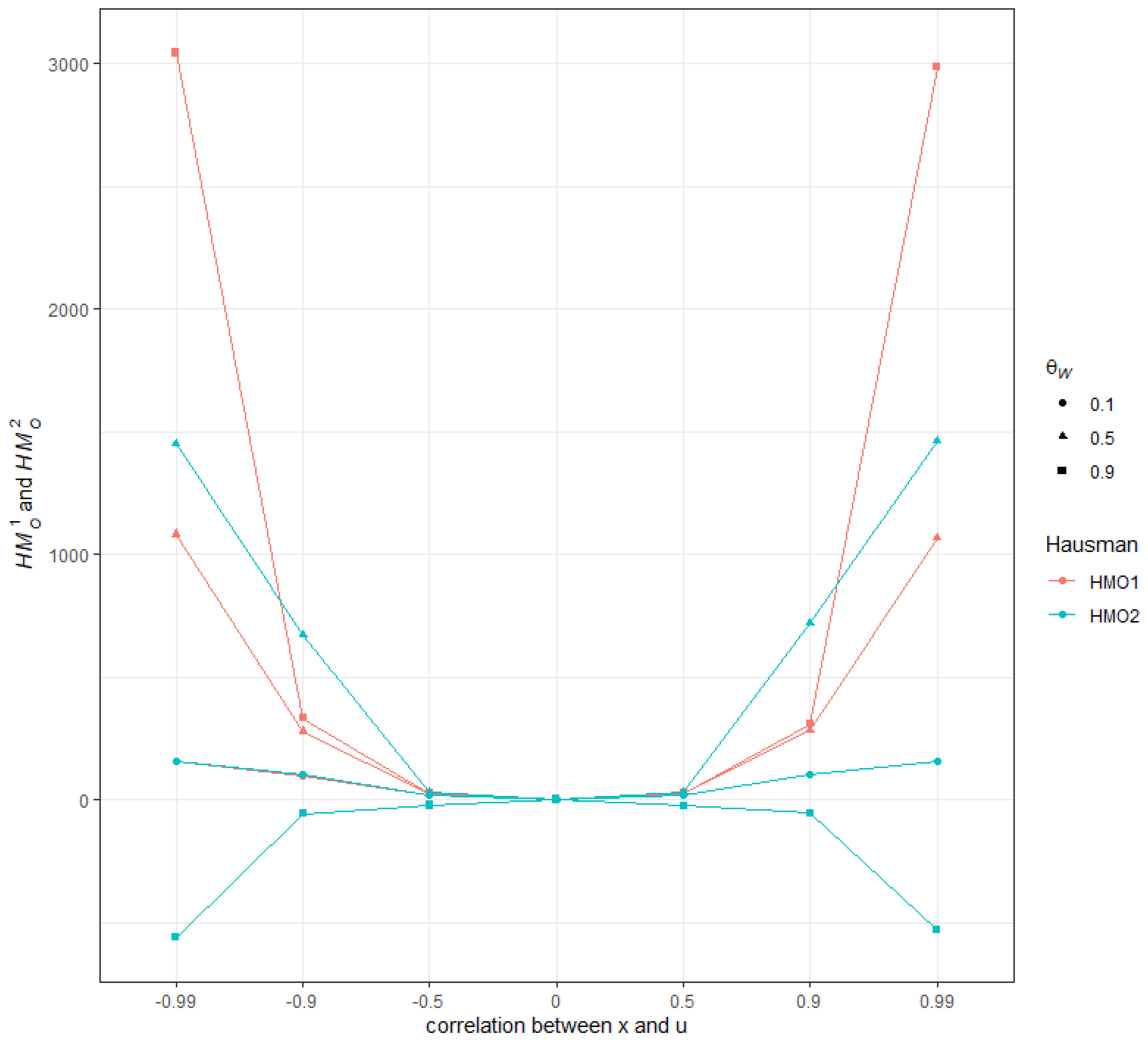
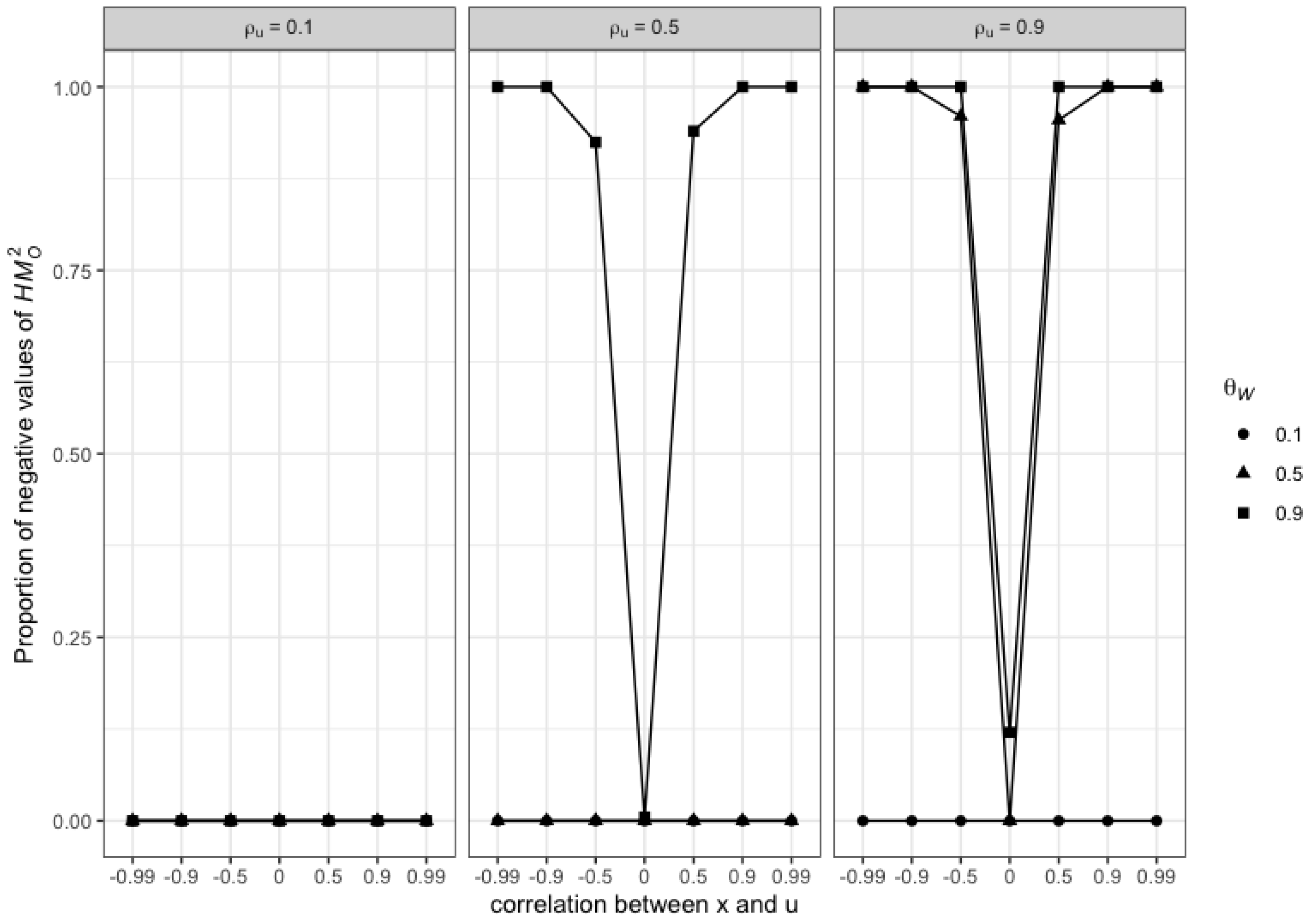
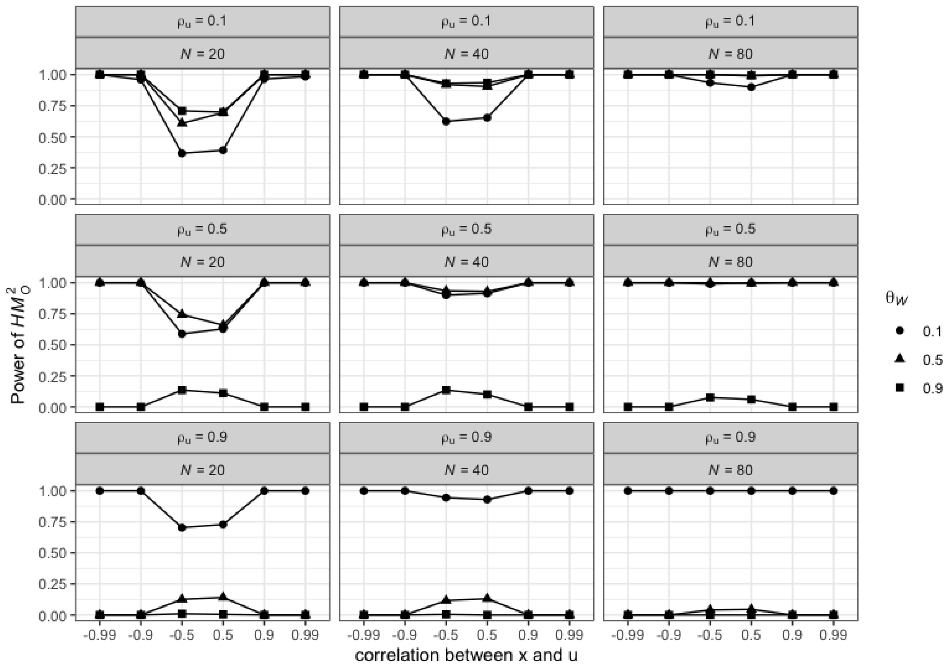
3.4.2. Illustrations in the Single Regressor Case

To illustrate the role of the previous factors as well as to clarify their interpretation, we perform Monte-Carlo simulations on the behavior of the main magnitudes involved in the comparison between ($H{M}_O^1$) and ($H{M}_O^2$) in a single-regressor model $(K=1)$.

Preliminary Results

In such a setting, $\mathbf{X}=\left\{\mathbf{x}\right\}$ and the various expressions for the main estimators and statistics simplify accordingly. We measure the total sample variance in the observations for $\mathbf{x}$ with $s_{\mathbf{x}}^2$ where $s_{\mathbf{x}}^2={(N·T)}^{-1}·{\mathbf{x}}_T^2$ and ${\mathbf{x}}_T^2\equiv {\mathbf{x}}^{\prime }·I_C·\mathbf{x}$, with $I_C\equiv I_{NT}-B_{NT}$. We then define ${\mathbf{x}}_W^2$$\equiv {\mathbf{x}}^{\prime }·W·\mathbf{x}$ and ${\mathbf{x}}_{B_C}^2\equiv {\mathbf{x}}^{\prime }·B_C·\mathbf{x}$. By construction, we have ${\mathbf{x}}_T^2={\mathbf{x}}_{B_C}^2+{\mathbf{x}}_W^2.$ Hence, ${\mathbf{x}}_W^2$ and ${\mathbf{x}}_{B_C}^2$ can be used as a measure of, respectively, the Within and the Between components (up to a $NT$- factor) of the total (empirical) variance in the NT observations contained in $\mathbf{x}$. Finally, define ${\theta }_W={\mathbf{x}}_W^2/{\mathbf{x}}_T^2$ the share of the Within variance in the total variance. Then, substituting, we obtain:

$$\begin{array}{cc}\hfill h_{min}=h_{max}\equiv h^{*}& =1+\frac{{\widehat{\psi }}^2·{\mathbf{x}}_{B_C}^2}{{\mathbf{x}}_W^2}=1+\frac{{\widehat{\psi }}^2·\left(1-{\theta }_W\right)}{{\theta }_W}\hfill \\ \hfill H{M}_O^1& =\nu ·{\mathbf{x}}_W^2·\frac{h^{*}}{h^{*}-1}\hfill \\ \hfill h& =1+\eta ·\left(\nu ·{\mathbf{x}}_W^2·\frac{h^{*}}{h^{*}-1}-1\right)\hfill \\ \hfill H{M}_O^2& =\nu ·{\mathbf{x}}_W^2·\frac{h^{*}}{h^{*}-h}\hfill \end{array}$$

with $\nu ={\left({\widehat{\sigma }}_{\epsilon }^2\right)}^{-1}·{\left({\widehat{\beta }}_{\Delta WRE}\right)}^2$ and $\eta =1/(NT-2)$.

Design of Simulations

We perform Monte-Carlo simulations on the behavior of the previous four quantities, $h{}^{*}$, h, $H{M}_O^1$ and $H{M}_O^2$. The details of the simulation design are presented in Appendix C. We generate several series of $y_{it}^a$ based on a model $y_{it}^a=\alpha +\beta ·x_{it}^a+u_{it}^a$, where we fix $\alpha =\beta =1$ and we let the other parameters of the simulation vary: $N=(20,40,80)$, $T=(20,40,80)$, $s_{\mathbf{x}}^2=(0.01,1,100)$, ${\theta }_W=(0.1,0.5,0.9)$, ${\sigma }_u^2=(0.01,1,100)$, ${\rho }_{xu}=(-0.99,-0.9,-0.5,0,0.5,0.9,0.99)$ and ${\rho }_u=(0.1,0.5,0.9)$ with the same notations as before, ${\rho }_{xu}$ is the correlation between x and u (on the cross-sectional dimension) and ${\rho }_u$ is the intra-class coefficient of the error term (share of the within variance in the total variance in u)17. Then, for each combination of the parameters, we perform 199 replications and compute the median of $H{M}_O^1$ and $H{M}_O^2$. To explore the main dimensions of variability of $H{M}_O^1$ and $H{M}_O^2$, we perform an ANCOVA analysis (

Table A2. ANCOVA on simulation results.

	Dependent Variable:
	Mean ${\mathit{HM}}_{\mathbf{0}}^{\mathbf{1}}$ (1)	Mean ${\mathit{HM}}_{\mathbf{0}}^{\mathbf{2}}$ (2)	Median ${\mathit{HM}}_{\mathbf{0}}^{\mathbf{1}}$ (3)	Median ${\mathit{HM}}_{\mathbf{0}}^{\mathbf{2}}$ (4)
$N=40$ (ref = 20)	−24.158	134.826 **	−24.132	136.294 **
	(37.475)	(56.029)	(36.677)	(55.435)
$N=80$ (ref = 20)	−72.354 *	405.306 ***	−72.281 **	409.057 ***
	(37.475)	(56.029)	(36.677)	(55.435)
$T=40$ (ref = 20)	63.206 ***	111.042 ***	60.953 ***	110.473 ***
	(16.759)	(25.057)	(16.402)	(24.791)
$T=80$ (ref = 20)	126.892 ***	306.754 ***	122.040 ***	303.316 ***
	(16.759)	(25.057)	(16.402)	(24.791)
${\mathbf{x}}_T^2=1$ (ref = 0.01)	0.039	−1.105	0.322	−0.300
	(16.759)	(25.057)	(16.402)	(24.791)
${\mathbf{x}}_T^2=100$ (ref = 0.01)	0.277	2.784	0.803	−0.171
	(16.759)	(25.057)	(16.402)	(24.791)
${\theta }_W=0.5$ (ref = 0.1)	90.452 ***	−18.134	83.656 ***	−16.453
	(29.028)	(43.400)	(28.410)	(42.940)
${\theta }_W=0.9$ (ref = 0.1)	184.362 ***	−35.323	167.161 ***	−30.374
	(29.028)	(43.400)	(28.410)	(42.940)
${\rho }_{xu}=-0.99$ (ref = 0)	1083.156 ***	640.633 ***	1057.507 ***	643.296 ***
	(25.600)	(38.275)	(25.055)	(37.869)
${\rho }_{xu}=-0.9$ (ref = 0)	147.213 ***	214.549 ***	141.792 ***	202.157 ***
	(25.600)	(38.275)	(25.055)	(37.869)
${\rho }_{xu}=-0.5$ (ref = 0)	13.481	14.882	12.514	5.921
	(25.600)	(38.275)	(25.055)	(37.869)
${\rho }_{xu}=0.5$ (ref = 0)	13.436	3.664	12.469	5.878
	(25.600)	(38.275)	(25.055)	(37.869)
${\rho }_{xu}=0.9$ (ref = 0)	147.237 ***	215.027 ***	141.974 ***	201.985 ***
	(25.600)	(38.275)	(25.055)	(37.869)
${\rho }_{xu}=0.99$ (ref = 0)	1083.935 ***	641.078 ***	1058.341 ***	643.762 ***
	(25.600)	(38.275)	(25.055)	(37.869)
${\sigma }_u^2=1$ (ref = 0.01)	−0.265	3.723	0.343	0.056
	(16.759)	(25.057)	(16.402)	(24.791)
${\sigma }_u^2=100$ (ref = 0.01)	0.400	0.780	1.234	−0.119
	(16.759)	(25.057)	(16.402)	(24.791)
${\rho }_u=0.5$ (ref = 0.1)	90.544 ***	−20.710	83.885 ***	−15.796
	(29.028)	(43.400)	(28.410)	(42.940)
${\rho }_u=0.9$ (ref = 0.1)	184.478 ***	−31.878	167.171 ***	−29.092
	(29.028)	(43.400)	(28.410)	(42.940)
$N=40$: ${\theta }_W=0.5$	86.977 **	−16.080	87.205 **	−15.864
	(41.052)	(61.376)	(40.177)	(60.726)
$N=80$: ${\theta }_W=0.5$	261.702 ***	−41.165	262.250 ***	−48.630
	(41.052)	(61.376)	(40.177)	(60.726)
$N=40$: ${\theta }_W=0.9$	175.791 ***	−27.656	176.433 ***	−30.434
	(41.052)	(61.376)	(40.177)	(60.726)
$N=80$: ${\theta }_W=0.9$	525.795 ***	−89.808	526.255 ***	−92.123
	(41.052)	(61.376)	(40.177)	(60.726)
$N=40$: ${\rho }_u=0.5$	86.826 **	−13.059	86.837 **	−16.015
	(41.052)	(61.376)	(40.177)	(60.726)
$N=80$: ${\rho }_u=0.5$	261.064 ***	−45.820	261.054 ***	−48.512
	(41.052)	(61.376)	(40.177)	(60.726)
$N=40$: ${\rho }_u=0.9$	175.736 ***	−30.548	176.043 ***	−31.087
	(41.052)	(61.376)	(40.177)	(60.726)
$N=80$: ${\rho }_u=0.9$	526.388 ***	−84.972	526.704 ***	−92.531
	(41.052)	(61.376)	(40.177)	(60.726)
Constant	−446.938 ***	−246.347 ***	−430.229 ***	−246.886 ***
	(35.552)	(53.154)	(34.795)	(52.590)
Observations	5103	5103	5103	5103
R2	0.580	0.165	0.579	0.169
Adjusted R2	0.578	0.161	0.577	0.165
Residual Std. Error (df = 5076)	488.758	730.740	478.346	722.994
F Statistic (df = 26; 5076)	269.238 ***	38.691 ***	268.675 ***	39.743 ***

Note: * $p<$0.1; ** $p<$0.05; *** $p<$0.01.

in Appendix C) where we regress, respectively, each of the means and medians on the levels of the different parameters and the interactions that we found significant.

Results of the Simulations

The results are similar whether we consider the mean or the medians over the replications of the levels of $H{M}_O^1$ and $H{M}_O^2$ for each combination of parameters. The value of $H{M}_O^1$ and $H{M}_O^2$ significantly depend on T, ${\theta }_W$, high absolute values of ${\rho }_{xu}$ and ${\rho }_u$. Conversely, the scale parameters ${\mathbf{x}}_T^2$ and ${\sigma }_u^2$ do not have a significant impact on $H{M}_O^1$ and $H{M}_O^2$.

The visual representation of the behavior of (the median) $H{M}_O^1$ and $H{M}_O^2$ for $N=80$, $T=80$, $s_{\mathbf{x}}^2={\sigma }_u^2=1$ and ${\rho }_u=0.5$ is in Figure 1. This illustrates the strong dependence of the values of the Hausman statistics on ${\theta }_W$ on the one hand and on the correlation between $\mathbf{x}$ and $\mathbf{u}$ on the other hand. In particular, for high absolute values of ${\rho }_{xu}$ and high values of ${\theta }_W$, $HM{O}_2$ even yields negative values.

This latter result is, for example, consistent with the regression outcomes obtained with $log\left[fuelprice\right]$ as a single covariate in the framework of motivating Example 2 [Airline]. In this case (see

Table A3. Estimation results for Motivating example 2, Airline, single covariate.

Specification		Intercept	$log\left[\mathit{fuelprice}\right]$
Within specification	Coef.	−	$0.7785$
	Std Err.	−	$0.0279$
Between specification	Coef.	$476.260$	$-36.248$
	Std Err.	$136.439$	$10.684$
Random effect specification	Coef.	$3.4264$	$0.7783$
	Std Err. 1	$0.4245$	$0.0279$
	Std Err. 2	$0.4502$	$0.0296$
${HM}_O^1$	$12.0100$
${HM}_O^2$	$-0.0006$
${\widehat{\sigma }}_{\epsilon }^2$	$0.0456$
${\widehat{\sigma }}_{\epsilon }^{*2}$	$0.0513$
${\widehat{\psi }}^2$	$0.0095$
h	$1.1251$
$h^{*}$	$1.0000$
${2·h}^{*}-1$	$1.0000$
Within variance			$0.6521$
Between variance			$0.0005$
Within variance/Total variance (in %)	${\theta }_W$		$99.9282$
Between variance/Total variance (in %)	${\theta }_B$		$0.0718$

), ${HM}_O^2$ is computed as a negative scalar with $H{M}_O^1>\left|H{M}_O^2\right|$. Note also the extremely large value of ${\theta }_W$ for the covariate which partly drives the values taken by $h^{*}$ and h.

Finally, looking more closely at the distribution of negative values for $H{M}_O^2$ (Figure A1 in Appendix C), we clearly see that they are an increasing function of ${\rho }_u$, ${\theta }_W$ and ${\rho }_{xu}$ (correlation between x and u) in absolute value. While the empirical size of both tests remains around $5\%$ with little variations for the various values of the parameters, the power of $H{M}_O^2$ consequently drops to 0 for the highest values of ${\rho }_u$, ${\theta }_W$ and ${\rho }_{xu}$ (Figure A2 in Appendix C).

4. The Implementation of the Hausman Test in Standard Econometric Software Packages for Panel Data: A Brief Review and Discussion

In this section, we review how six well-known econometric software packages deal with the implementation of the Hausman test in a standard panel data model and provide some discussion.

4.1. Review

• STATA programming commands for the estimation of the random-effects panel data models (xtreg with the re option) rely on the specification of the quasi-demeaned model in (8). As a consequence, the random effects parameter estimates as well as its “conventional” covariance matrix estimate are provided as standard outputs of the OLS regression performed on that model. In particular, the vce(conventional) - default - command yields the (asymptotic) covariance matrix estimate based on the standard variance estimator for OLS regression. This corresponds to $\mathbf{v}\widehat{\mathbf{a}}{\mathbf{r}}_2\left[{\widehat{\beta }}_{FGLS}\right]$ with, accordingly, ${\widehat{\sigma }}_{\epsilon }^{*2}$ used for the residual variance estimate. The default version of the command for implementing the standard Hausman test (the hausman command) corresponds accordingly to $H{M}_O^2$.
• The R PLM package developed by Croissant and Millo (2008) allows estimating a wide range of panel data models with R software. Regarding the random-effects specification, the estimation process can be implemented via the plm function, whose model argument takes the random option. Croissant and Millo (2008) point out that it could have been possible to program the computation of the covariance matrix estimator for ${\widehat{\beta }}_{FGLS}$ directly from the formula (11), “once the variance components have been estimated and hence the covariance matrix of errors”. However, to limit the computational costs associated with the inversion of the ($NT\times NT$) matrix ($\widehat{\Omega }$) or ($\widehat{{\Omega }_C^{*}}$) and the related memory limits to store it, plm resorts to the specification and estimation of the quasi-demeaning estimator (8). Then, the coefficients’ covariance matrix estimator is readily calculated by applying the standard OLS formulas which, in the R language, go through the vcov() command.
  The phtest command computes the Hausman test in plm. Its main arguments are the two-panel model objects that underlie the comparison (ex. model = within and model = random). The corresponding estimates of the asymptotic covariances matrices provided under both models are thus used to compute the Hausman statistic corresponding to $H{M}_O^2$.
• EViews estimates the random effects models using feasible GLS. The first step refers to the estimation of the covariance matrix for the composite error formed by the effects and the idiosyncratic disturbance. The EViews 9 User’s Guide II notes “Once the component variances have been estimated, we form an estimator of the composite residual covariance, and then GLS transform the dependent and regressor data”. As for the computation of the FGLS estimate, Eviews uses the quasi-demeaned model specification and proceeds on this basis. However, the calculation of the related coefficients’ covariance matrix is based on the direct application of the formula (11) and thus corresponds to $\mathbf{v}\widehat{\mathbf{a}}{\mathbf{r}}_1\left[{\widehat{\beta }}_{FGLS}\right]$. The procedure for the Hausman test then corresponds to $H{M}_O^1$.
• MATLAB provides estimation methods for the standard fixed (Within), between, and random effects models with the the panel data toolbox. Panel data models are estimated using the panel(·) function with the options argument set to re for the random effects model specification. The random effects FGLS estimates are based on the quasi-demeaned model and the asymptotic variance-covariance matrix for statistical inference is accordingly provided by $\mathbf{v}\widehat{\mathbf{a}}{\mathbf{r}}_2\left[{\widehat{\beta }}_{FGLS}\right]$ (see Equation (18) in Alvarez et al. (2017)). Then, hausmantest computes the Hausman test where the input of the hausmantest function requires the output structures of the two estimations to be compared. Accordingly, the statistics that are computed correspond to $H{M}_O^2$.
• GAUSS: The GAUSS Times Serie∞s MT 3.0 TSMT provides a fixed effects and random effects models (TSCS) package that can be implemented through the tsmt library and the one-in-all tscsFit procedure. Another possibility is to use the pdlib GAUSS library and the randomEffects procedure in it. Both procedures implement the quasi-demeaning transformation on the original dataset and apply the standard OLS estimator on the transformed data so as to form the FGLS estimate. The covariance matrix estimate comes as a direct by-product of the OLS outcome so that $\mathbf{v}\widehat{\mathbf{a}}{\mathbf{r}}_2\left[{\widehat{\beta }}_{FGLS}\right]$ is used. The Hausman test provided in the tscsFit procedure is implemented accordingly and corresponds to $H{M}_O^2$.
• SAS (SAS ETS 13.2) provides estimation methods for the standard fixed (Within), between, and random effects models in the balanced and unbalanced cases with the PANEL procedure toolbox. Standard panel data models are estimated using the PROC PANEL command with the MODEL statement specifying the regression model and the assumptions for the error structure. Specifically, FIXONE and RANONE must be used to specify the fixed-effect and the random-effect models, respectively (in the cross-sectional one-way case). In the latter case, various methods (but not the Swamy-Arora approach) are proposed to estimate, in the first stage, the variance components (through the VCOMP = option). It is explicitly indicated that the random effects FGLS estimates are then based, in the balanced case, on these variance components estimates through the quasi-demeaning approach, where ‘the random effects $\beta$ is then the result of simple OLS on the transformed data’ (see SAS ETS 13.2 User Manual (2014), p. 1417). The estimator for the asymptotic variance-covariance matrix is thus provided by $\mathbf{v}\widehat{\mathbf{a}}{\mathbf{r}}_2\left[{\widehat{\beta }}_{FGLS}\right]$. The Hausman statistic is automatically generated and reported as a conventional F statistic, with the statistic computed as $H{M}_O^2$.

4.2. Discussion

As the previous review indicates, in all but one of the packages discussed above, the Hausman test is, by default, implemented through the computation of $H{M}_O^2$ with the quasi-demeaning estimator. The rationale for such a choice is computational. Indeed, the quasi-demeaning approach allows avoiding the inversion of the ($NT\times NT$) matrix $\widehat{\Omega }$ or ${\Omega }_C^{*}$, which can be computationally costly (in terms of time and rounding errors). Conversely, the quasi-demeaned model only requires partially demeaning the variables with $\theta \equiv 1-\widehat{\psi }$ as the partial demeaning factor. Yet, as a counterpart of this standard OLS regression, ${\widehat{\sigma }}_{\epsilon }^{*2}$ is naturally chosen to compute the residual variance estimate and, in turn, yields to $H{M}_O^2$, which might, as we have seen, be an unreliable statistic for the Hausman test. In what follows, we explore some ways to circumvent the problems posed by the use of this statistic.

(1) First, it is possible to compute $H{M}_O^1$ and still rely on the quasi-demeaning approach to estimate the parameters of the RE model (which, as mentioned before, is the default case in the vast majority of available econometric software). This can been easily seen from the relationship (21) that we established between h and $H{M}_O^1$. Once h has been determined, which only requires the OLS residual sums of squares from the estimation of the Within and the quasi-demeaning estimator, we can derive $H{M}_O^1$. Hence, the following procedure can be suggested, if required, to supplement the existing programs.

• Use the quasi-demeaning estimator to compute the RE estimator for $\beta$ and ${\widehat{\sigma }}_{\epsilon }^{*2}$.
• Use ${\widehat{\sigma }}_{\epsilon }^{*2}$ and ${\widehat{\sigma }}_{\epsilon }^{w2}$ (within regression) to compute h.
• Rearranging (21), obtain $H{M}_O^1$ from h as: $H{M}_O^1=\left(NT-\left(K+1\right)\right)·\left(h-1\right)+K$.
• Implement the Hausman test on the basis of $H{M}_O^1.$

(2) Second, depending on the software packages considered, some programming options can be used to fix the potential ‘variance disconnect’ problem associated with the use of the statistic $H{M}_O^2$.

For example, in STATA, it is possible to use the sigmamore and/or sigmaless option commands when implementing the Hausman test. As indicated in STATA instructions: “sigmamore and sigmaless specify that the two covariance matrices used in the test be based on a common estimate of disturbance variance. sigmamore specifies that the covariance matrices be based on the estimated disturbance variance from the efficient estimator. sigmaless specifies that the covariance matrices be based on the estimated disturbance variance from the consistent estimator”. Following the lines of Hausman’s seminal approach would lead to the choice of sigmaless option, whereby the variance estimator, is based on the Within model, would be used18. This would ensure the test to be performed upon the $H{M}_0^1$ statistics. The choice of sigmamore19 would imply to consider a third test statistics, $H{M}_0^3$, where the common disturbance variance estimator would be based on the quasi-demeaned model, so that we would have: $H{M}_O^3={\widehat{\beta }}_{\Delta WRE}^{\prime }·{\left({\widehat{\sigma }}_{\epsilon }^{*2}·\Gamma \right)}^{-1}·{\widehat{\beta }}_{\Delta WRE}$. Comparing $H{M}_O^3$ and $H{M}_O^1$, we observe that $H{M}_0^1>H{M}_0^3$ whenever $h<1$. Thus, the more likely it would be to favor (even unduly) the rejection of the null hypothesis on the basis of $H{M}_0^3$ when $h>1$.

Some packages also offer the possibility to rely on an alternative expression for the Hausman statistic that does not involve the use of the RE estimator, so that it is immune to the variance disconnect problem. This expression was initially proposed by Hausman and Taylor (1981) and is based on the difference between the Between and Within estimators ${\widehat{q}}^{**}\equiv {\widehat{\beta }}_W-{\widehat{\beta }}_B$. Hausman and Taylor (1981, pp. 1382–83), establish that the resulting version of the Hausman statistic is numerically exactly identical to the one that is built upon $\widehat{q}$ and used above, that is: ${\widehat{q}}^{\prime }·{\left[\mathbf{var}\left(\widehat{q}\right)\right]}^{-1}·\widehat{q}={\widehat{q}}^{**\prime }·{\left[\mathbf{var}\left({\widehat{q}}^{**}\right)\right]}^{-1}·{\widehat{q}}^{**}$. Such a solution can be notably implemented in the R PLM package using the phtest command and specifying as arguments model = within and model = between.

(3) Finally, two other approaches that depart from the separate estimation of the FE and RE model parameters - which underlies the standard implementation of the Hausman test - can be emphasized. They have the advantage of solving the disturbance variance estimator disconnect problem, while allowing, more generally, for a robust implementation of the Hausman test20.

(3.1) The first of these approaches relies on implementing an auxiliary regression, that was initially proposed by Hausman himself together with the presentation of the standard specification test (see also Mundlak 1978). This regression takes the following form:

$${\tilde{\mathbf{y}}}_{**}={\tilde{\mathbf{Z}}}_{**}·\delta +{\mathbf{X}}_W·\gamma +\eta$$

with ${\tilde{\mathbf{Z}}}_{**}\equiv \left[{\tilde{\omega }}_{**}⋮{\tilde{\mathbf{X}}}_{**}\right]$ where ${\tilde{\omega }}_{**}$$\equiv \widehat{\psi }·{\iota }_{NT}$ and ${\tilde{\mathbf{X}}}_{**}\equiv$${\widehat{{\Omega }^{*}}}^{-\frac{1}{2}}·\mathbf{X};{\tilde{\mathbf{y}}}_{**}\equiv {\widehat{{\Omega }^{*}}}^{-\frac{1}{2}}·\mathbf{y}$ and $\eta$ a vector of standard random disturbances.

It can be shown that the formula of the standard Wald test statistic for testing whether $\gamma =\mathbf{0}$ in the previous regression framework is equivalent to the one of the standard Hausman test statistic as expressed in terms of the difference between the Between and Within estimators (see Hausman and Taylor 1981 and above)21. Resorting to this auxiliary regression framework has two advantages. First, it involves only one estimator for the covariance matrix in the Wald test statistic formula, that one for $\gamma$, which is immune to the positive definiteness problem that can be encountered with the standard Hausman test statistic. Second, and as underlined by Baltagi and Liu (2007), it can be made robust to heteroskedasticity of unknown form (see, also, Arellano 1993).22 Once the variables have been transformed to be included as regressors in the auxiliary regression framework, the latter can be implemented in a rather standard way in any of the software econometric packages we have reviewed supra.

(3.2) The second approach goes through implementing White (1982)’s reformulated Hausman specification test that is based on the Maximum Likelihood (ML) estimation of the FE and RE model parameters. The related test statistic takes the form:

$$HW=n·{\left({\tilde{\beta }}_{MLE}^W-{\tilde{\beta }}_{MLE}^{RE}\right)}^{\prime }·\tilde{S}·\left({\tilde{\beta }}_{MLE}^W-{\tilde{\beta }}_{MLE}^{RE}\right)$$

with $n\equiv \left(N·T\right)$ and ${\tilde{\beta }}_{MLE}^W$ (resp. ${\tilde{\beta }}_{MLE}^{RE}$) denoting the ML estimator related to the Within (resp RE) regression framework; $\tilde{S}$ would serve as the covariance matrix estimator and involves the information matrices for both estimators of $\beta$, as well as outer products of scores within and between the two models under concern. White (1982) shows that $\tilde{S}$ remains positive definite even under misspecification (including heteroskedasticity).

The last two procedures we have presented could even be suggested to be used in the first place when assessing the relevance of the RE-model specification as they allow for globally robust implementation of the Hausman test in the context of panel data models (if only, insofar as they do not require to be directly based on the use of the RE (FGLS) disturbance variance estimator).

5. Conclusions

In this paper, we provide new analytical results of the behavior of the Hausman statistic for the test of orthogonality between the individual effects and the error term in a static and balanced panel data model. We compare the Hausman statistic computed with direct FGLS implementation and the Hausman statistic computed on the quasi-demeaned model. We show that this difference depends upon several parameters; in particular, the between-within structure of the regressors. We show by means of a Monte Carlo simulation in the single regressor case and of a set of well-known textbook examples that the difference can be substantial and that in some cases, the Hausman statistic computed on the basis of the quasi-demeaned model can yield strong negative values. Therefore, despite its computational advantage, the quasi-demeaned model should not be used prima facie as the basis of the computation of the Hausman statistic. We suggest, if needed, to supplement the existing software instructions so as to be able to compute in any case the relevant statistic. Extensions can include deriving these analytical results for unbalanced panel data models, two-way component models and dynamic panel models.

References

1. Alvarez, Inmaculada C., Javier Barbero, and José L. Zofío. 2017. A Panel Data Toolbox for MATLAB. Journal of Statistical Software 76: 1–17. [Google Scholar] [CrossRef]
2. Amemiya, Takeshi. 1971. The Estimation of the Variances in a Variance-Components Model. International Economic Review 12: 1–13. [Google Scholar] [CrossRef]
3. Arellano, Manuel. 1993. On the testing of correlated effects with panel data. Journal of Econometrics 59: 87–97. [Google Scholar] [CrossRef]
4. Axler, Sheldon. 2014. Linear Algebra Done Right. New York: Springer. [Google Scholar]
5. Baltagi, Badi H. 2005. Econometric Analysis of Panel Data, 3rd ed. Chichester and Hoboken: J. Wiley & Sons. [Google Scholar]
6. Baltagi, Badi H. 2021. Econometric Analysis of Panel Data, 6th ed. Springer texts in Business and Economics. Cham: Springer. [Google Scholar] [CrossRef]
7. Baltagi, Badi H., and James M. Griffin. 1973. Gasoline demand in the oecd: An application of pooling and testing procedures. European Economic Review 22: 626–32. [Google Scholar] [CrossRef]
8. Baltagi, Badi H., and Long Liu. 2007. Alternative ways of obtaining Hausman’s test using artificial regressions. Statistics & Probability Letters 77: 1413–17. [Google Scholar] [CrossRef]
9. Baum, Christopher F., Mark E. Schaffer, and Steven Stillman. 2003. Instrumental Variables and GMM: Estimation and Testing. The Stata Journal: Promoting Communications on Statistics and Stata 3: 1–31. [Google Scholar] [CrossRef]
10. Cameron, Adrian Colin, and Pravin K. Trivedi. 2009. Microeconometrics Using Stata. College Station: Stata Press. [Google Scholar]
11. Cornwell, Christopher, and Peter Rupert. 2008. Efficient estimation with panel data: An empirical comparison of instrumental variable estimators. Journal of Applied Econometrics 3: 149–55. [Google Scholar]
12. Croissant, Yves, and Giovanni Millo. 2008. Panel Data Econometrics in R: The plm Package. Journal of Statistical Software 27: 1–43. [Google Scholar] [CrossRef]
13. Fuller, Wayne A., and George E. Battese. 1973. Transformations for Estimation of Linear Models with Nested-Error Structure. Journal of the American Statistical Association 68: 626–32. [Google Scholar] [CrossRef]
14. Fuller, Wayne A., and George E. Battese. 1974. Estimation of linear models with crossed-error structure. Journal of Econometrics 2: 67–78. [Google Scholar] [CrossRef]
15. Greene, William. 1999. Frontier Production Functions. In Handbook of Applied Econometrics Volume II: Microeconomics. Edited by Pesaran M. Hashem and Schmidt Peter. Oxford: Blackwell Publishing Ltd., pp. 75–153. [Google Scholar] [CrossRef]
16. Greene, William. 2000. Econometric Analysis, 4th ed. Upper Saddle River: Prentice Hall Internat. [Google Scholar]
17. Greene, William. 2012. Econometric Analysis, 7th ed. Pearson Series in Economics; Boston and Munich: Pearson. [Google Scholar]
18. Hausman, Jerry A. 1978. Specification Tests in Econometrics. Econometrica 46: 1251–71. [Google Scholar] [CrossRef]
19. Hausman, Jerry A., and William E. Taylor. 1981. Panel data and unobservable individual effects. Econometrica 49: 1377–98. [Google Scholar]
20. Hayashi, Fumio. 2000. Econometrics. Princeton: Princeton University Press. [Google Scholar]
21. Holly, Alberto. 1982. A Remark on Hausman’s Specification Test. Econometrica 50: 749–60. [Google Scholar] [CrossRef]
22. Maddala, Gangadharrao Soundalyara. 1971. The Use of Variance Components Models in Pooling Cross-Section and Time Series Data. Econometrica 39: 341–57. [Google Scholar]
23. Mundlak, Yair. 1978. On the pooling of time series and cross section data. Econometrics 46: 69–85. [Google Scholar]
24. Nerlove, Marc. 1971. A Note on Error Components Models. Econometrica 39: 383–96. [Google Scholar] [CrossRef]
25. Schreiber, Sven. 2008. The Hausman Test Statistic Can Be Negative even Asymptotically. Jahrbücher für Nationalökonomie und Statistik 228: 394–405. [Google Scholar] [CrossRef]
26. Staiger, Douglas, and James H. Stock. 1997. Instrumental Variables Regression with Weak Instruments. Econometrica 65: 557–86. [Google Scholar] [CrossRef]
27. Swamy, Paravastu Aananta Venkata Bhattandha, and Swarnjit S. Arora. 1972. The Exact Finite Sample Properties of the Estimators of Coefficients in the Error Components Regression Models. Econometrica 40: 261–75. [Google Scholar] [CrossRef]
28. Wallace, T. Dudley, and Ashiq Hussain. 1969. The Use of Error Components Models in Combining Cross Section with Time Series Data. Econometrica 37: 55. [Google Scholar] [CrossRef]
29. White, Halbert. 1982. Maximum Likelihood Estimation of Misspecified Models. Econometrica 50: 1–25. [Google Scholar] [CrossRef]
30. Wooldridge, Jeffrey M. 2010. Econometric Analysis of Cross Section and Panel Data, 2nd ed. Cambridge, MA: MIT Press. [Google Scholar]
Figure 1. Distribution of the median of H M O 1 and H M O 2 , N = 80 , T = 80 , s x 2 = σ u 2 = 1 and ρ u = 0.5 .
Econometrics 11 00025 g001