
Dirichlet Process Log Skew-Normal Mixture with a Missing-at-Random-Covariate in Insurance Claim Analysis

Abstract
:1. Introduction
- RQ1. If an additional unobservable heterogeneity is introduced by the inclusion of covariates, then what is the best method to capture the within-cluster heterogeneity in modeling the total losses, comparing several conventional approaches?
- RQ2. If an additional estimation bias results from the use of the incomplete covariates under missing-at-random (MAR) conditions, then what is the best way to increase the imputation efficiency, comparing several conventional approaches?
- RQ3. If an individual loss is distributed with log-normal densities, then what is the best way to approximate the sum of the log-normal outcome variables, comparing several conventional approaches?
2. Discussion on the Research Questions and Related Work
2.1. Can the Dirichlet Process Capture the Heterogeneity and Bias? RQ1 and RQ2
2.2. Can a Log Skew-Normal Mixture Approximate the Log-Normal Convolution? RQ3
2.3. Our Contributions and Paper Outline
3. Model: DP Log Skew-Normal Mixture for
3.1. Background
- : the parameters of the outcome variable defined by cluster j.
- : the parameters of the covariates defined by cluster j.
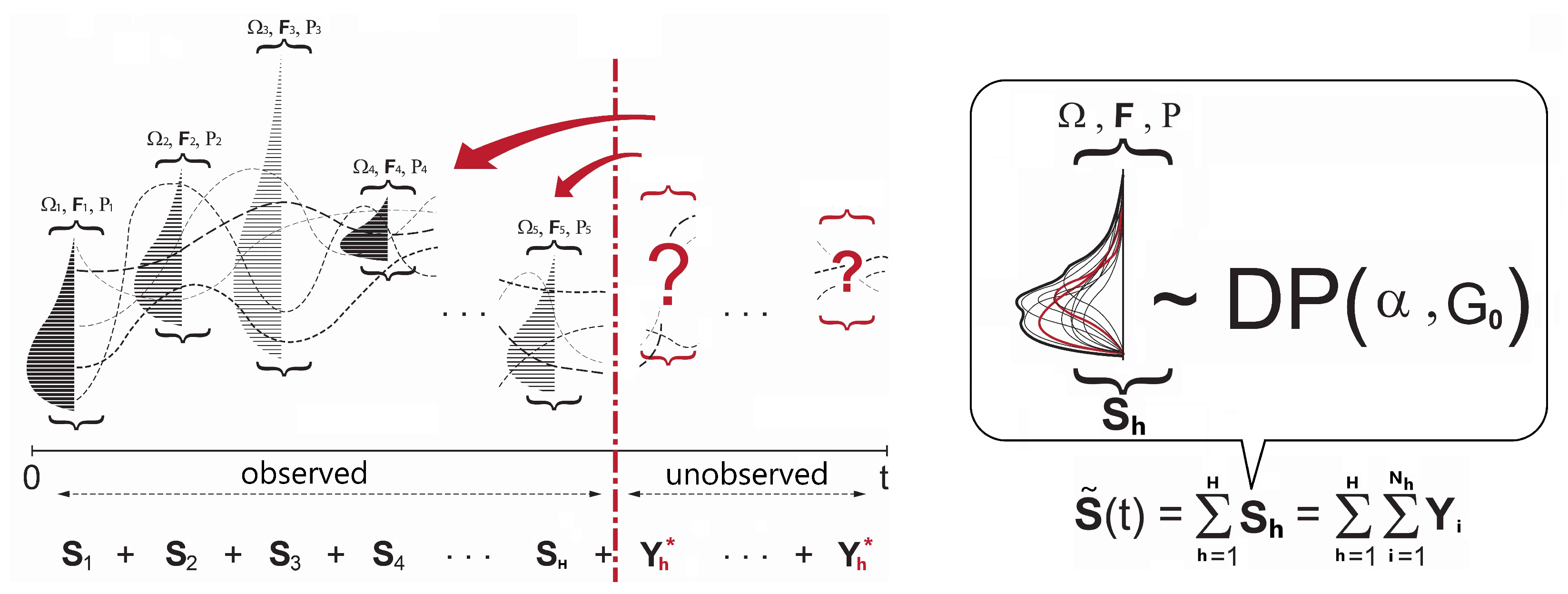
3.2. Model Formulation with Discrete and Continuous Clusters
3.3. Modeling with a Complete Case Covariate
- Stage 1.
- Cluster membership update:
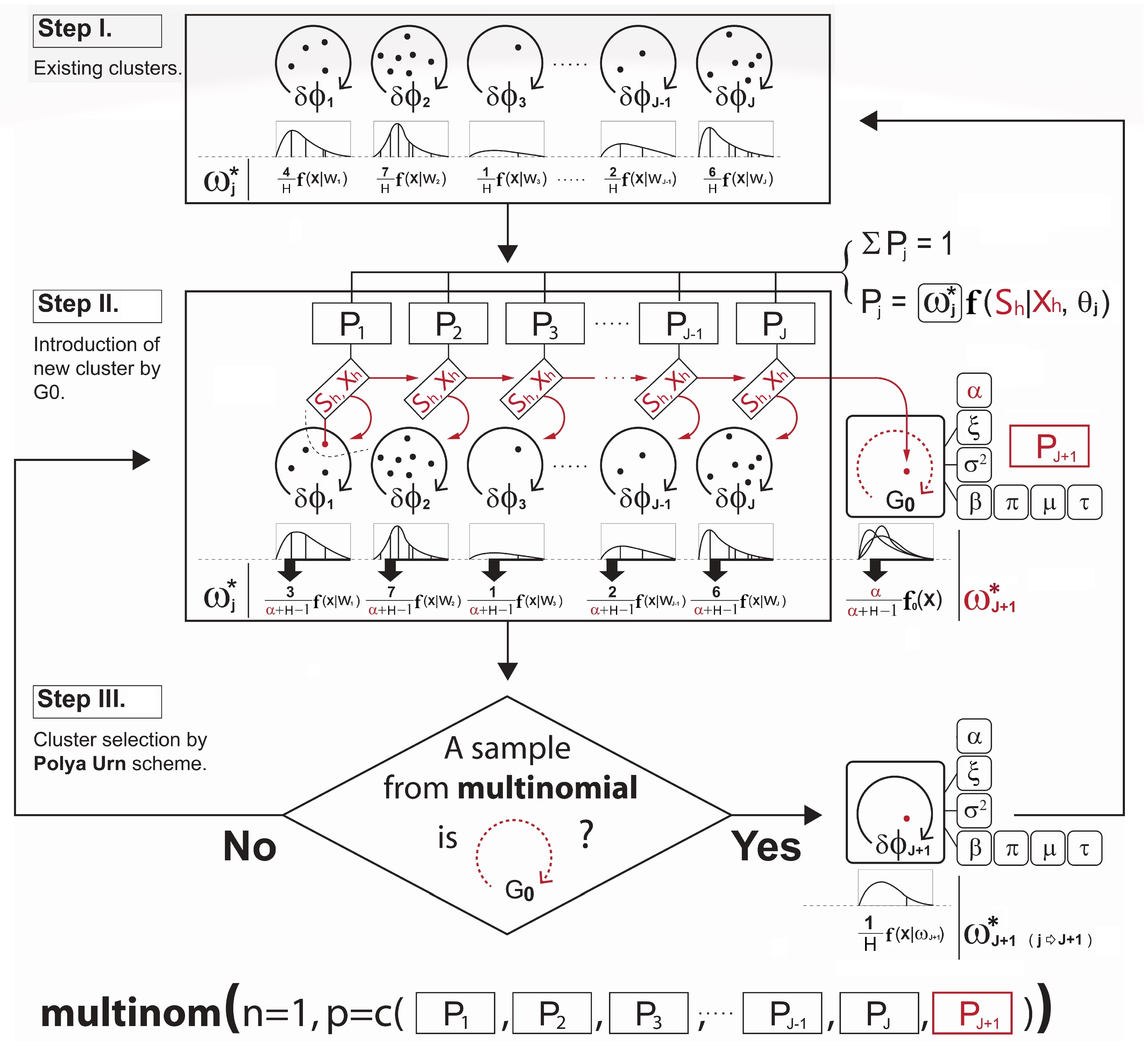
- Step I.
- Let the cluster-index for the observation h be . First, the cluster membership j is initialized by some clustering methods such as hierarchical or k-means clustering. This provides an initial clustering of the data ( as well as the initial number of clusters.
- Step II.
- Next, with the parameters sampled from the DPM prior described in Section 4.1 and the conditional probability term on lines 6 and 9 in Algorithm A2 for the observation assignment, the ultimate probabilities of the selected observation h being in the current discrete clusters and the proposed continuous cluster are computed, respectively. (The use of such a nonparametric prior to the development of a new continuous cluster allows the shape of the cluster to be driven by the data). Note that the term is known as the Chinese Restaurant process (see Blei and Frazier 2011) probability given bywhere c is a scaling constant to ensure that the probabilities add up to one and is the collection of cluster indices assigned to every observation without the cluster index of the observation h. A larger results in a higher chance of developing the new continuous cluster and adding to the collection of the existing discrete clusters. Since the number of clusters is not fixed, and the sequence of cluster assignment to observation cannot be ordered, one might be concerned about the sampling variance or convergence problem in the Gibbs sampler. In this regard, we expect that Equation (7) can carry out stable simulations with the Gibbs sampler. Neal (2000) pointed out that from the example of Escobar’s algorithm, the sequence in which the observation h arrives in the cluster is exchangeable under this conditional probability distribution described in Equation (7). This means that the ultimate joint distribution to update the cluster memberships from lines 4 to 10 in Algorithm A2 does not depend on the order of the sequence in which the observations arrive.
- Step III.
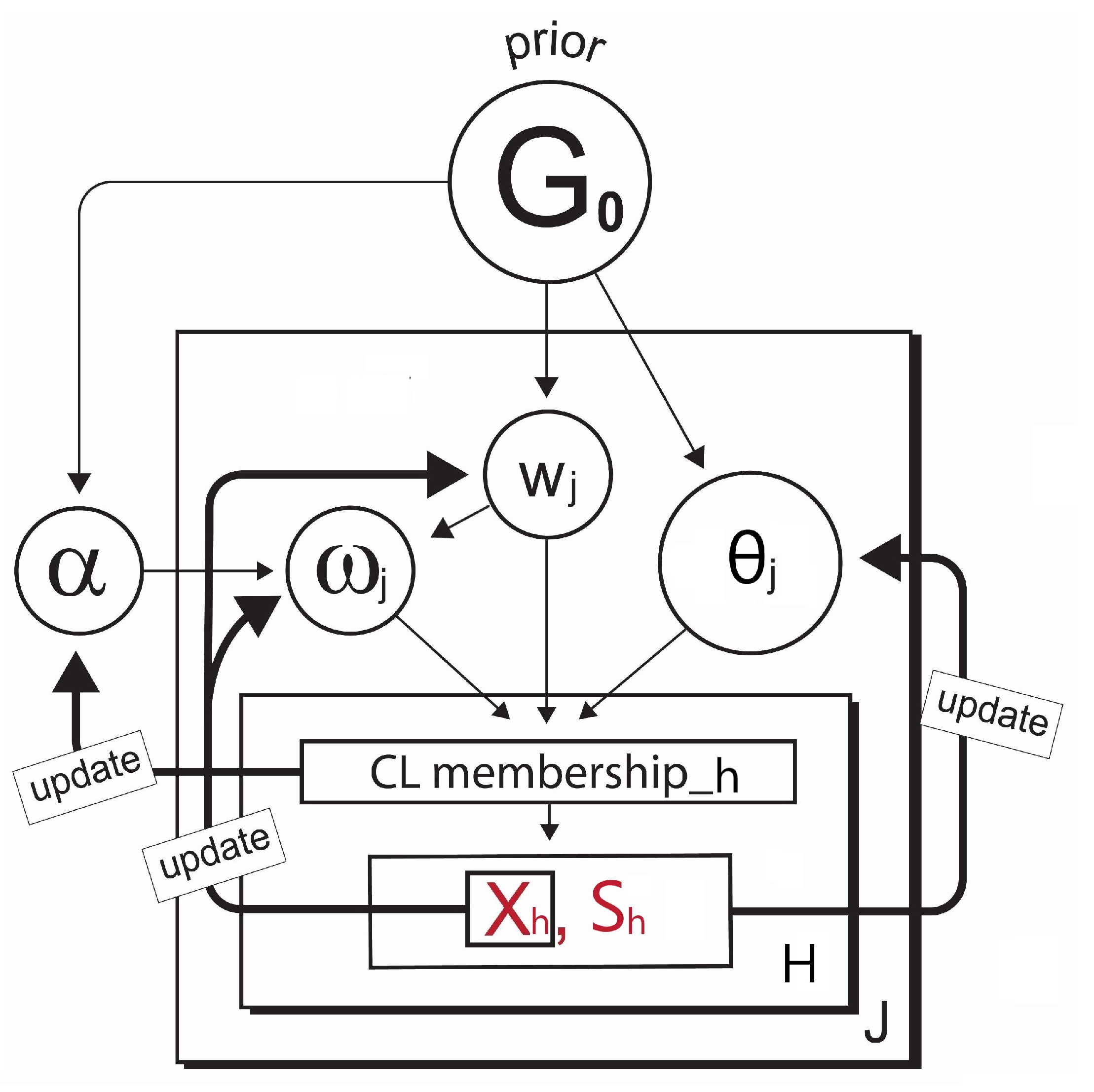
- Lastly, the new cluster membership is determined and updated by the Polya Urn scheme using a multinomial distribution based on the resulting cluster probabilities. This is briefly illustrated in Figure 2. Please note how the development of the cluster weighting components in Equations (6a) and (6b) is made in Figure 2.
- Stage 2.
- Parameter update:
- Once all observations have been assigned to particular clusters at a given iteration in the Gibbs sampling, the parameters of our interest— and —for each cluster are updated, given the new cluster membership. This is accomplished using the posterior densities denoted by , and , in which represents all observations in cluster j. When it comes to the forms of the prior and posterior densities from lines 17 to 23 in Algorithm A2 that are used to simulate the parameters , we detail them in Appendix A.
3.4. Modeling with the MAR Covariate
- (a)
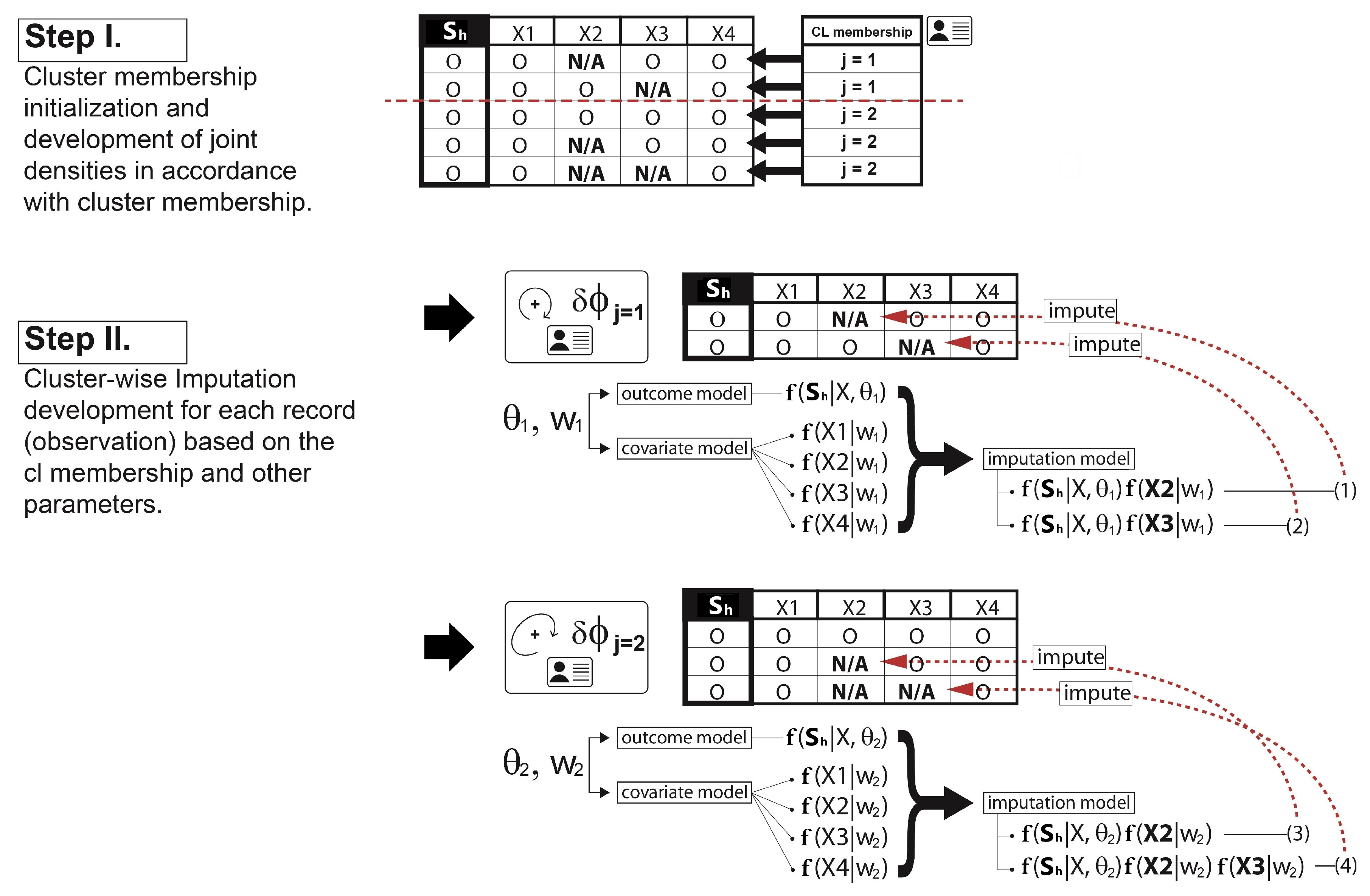
- Adding an imputation step in the parameter update stage:It is true that the missing covariate impacts on the parameter——update. For the parameters for the covariates , only the observations h without the missing covariate are used for updating. If the cluster does not have any observations with complete data for that covariate, then a draw from the prior distribution for would be used to update it. For the parameters for the outcome , however, we must first impute values for the missing covariates for all observations h within the cluster j. Since we already defined a full joint model——in Section 3.2, we can obtain draws for the MAR covariate from the imputation model, such asat each iteration in the Gibbs sampling. Each imputation model is proportional to the joint distribution as a product of the outcome model and the covariate model that has missing data. The imputation process is illustrated in depth in Figure 3. Once all missing covariate values have been imputed, then the parameters of each cluster are recalculated and sampled from the posterior of . After this cycle is complete in the Gibbs sampling, the imputed data are discarded, and the same imputation steps are repeated for every iteration.
- (b)
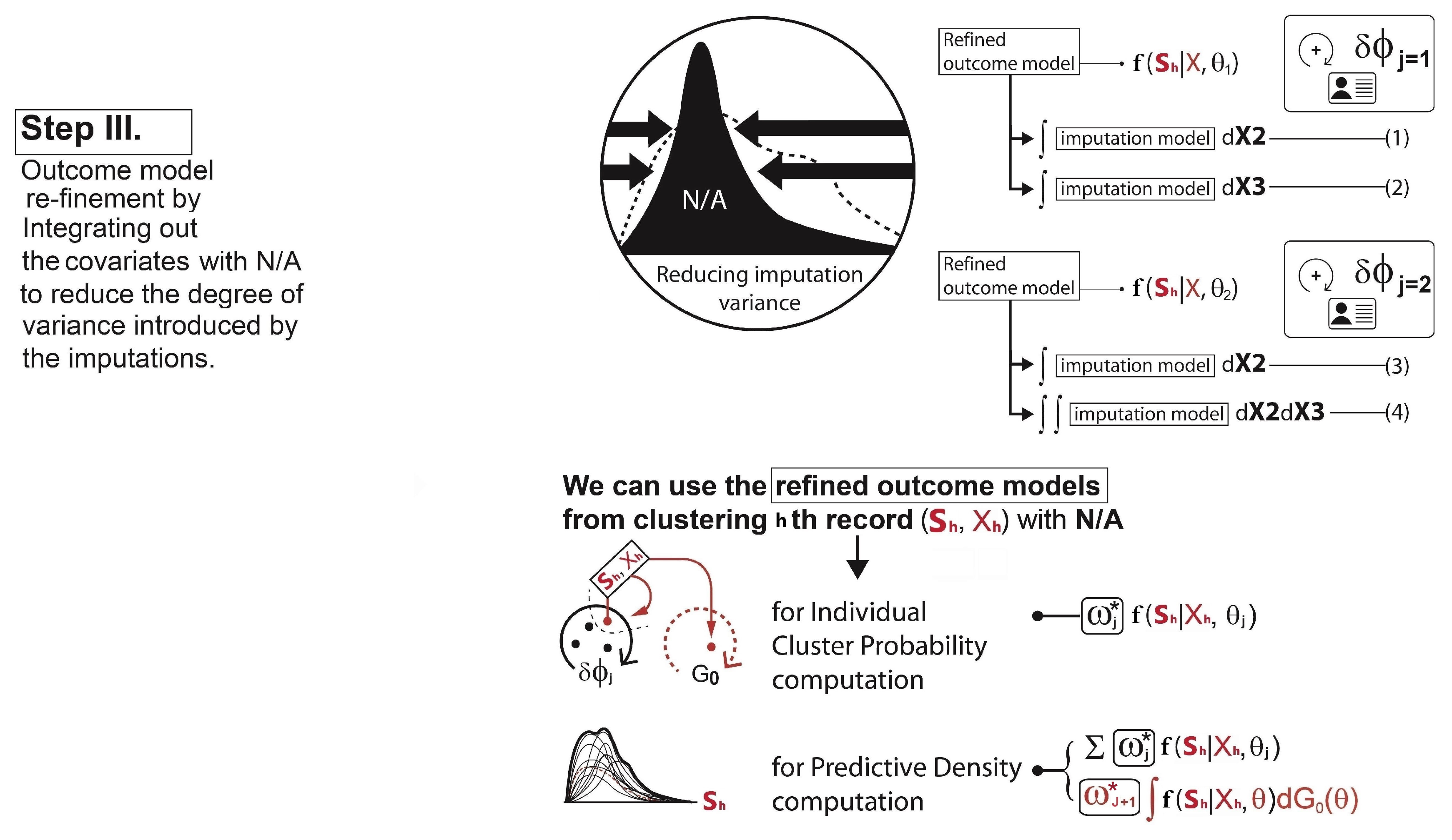
- Adding a reclustering step in the cluster membership update stage:To calculate each cluster probability after the parameter updates, the algorithm redefines the two main components: (1) the covariate model and (2) the outcome model. For the covariate model , we set this equal to the density functions of only those covariates with complete data for observation h. Assuming that , and the covariate is missing for observation h, then we drop and only use in the covariate model:This is the refined covariate model for the cluster j with the observation h, where the data in are not available. For the outcome model , the algorithm simply takes the imputation model in Equation (8) for the observation h and integrates it out of the covariates with missingness . This reduces the degrees of variance introduced by the imputations. In other words, as the covariate is missing for observation h, this missing covariate can be removed from the term that it is being conditioned on. Therefore, the refined outcome model isThe same process is performed for each observation with missing data and each combination of missing covariates. Hence, using Equations (9) and (10), the cluster probabilities and the predictive distribution can be obtained as illustrated in Step III in Figure 4.
- (c)
- Re-updating the parameters:The cluster probability computation is followed by the parameter reestimation for each cluster, which is illustrated via the diagram in Figure 5. This is the same idea as what we have discussed about the parameter () update in Section 3.3.
3.5. Gibbs Sampler Modification in Detail for the MAR Covariate
- (a)
- (b)
- (c)
- In line 22, with the presence of a missing covariate , the imputation should be made before simulating the parameter as follows:The imputation model formulation above was discussed in Section 3.4.
4. Bayesian Inference for with the MAR Covariate
4.1. Parameter Models and the MAR Covariate
4.2. Data Models and the MAR Covariate
- (a)
- Covariate model for the discrete clusterFocusing on the scenario where is binary, is Gaussian, and the only covariate with missingness is , we simply drop the covariate to develop the covariate model for the discrete cluster. For instance, when computing the covariate probability term for the hth observation in cluster j, the covariate model simply becomes due to the missingness of . As we have , which is assumed to be normally distributed as defined in Equation (1), its probability term isinstead of
- (b)
- Covariate model for the continuous clusterIf the binary covariate is missing, then by the same logic, we drop the covariate for the continuous cluster. However, using Equation (4), the covariate model for the continuous cluster integrates out the relevant parameters simulated from the Dirichlet process prior as follows:instead ofThe derivation of the distributions above is provided in Appendix C.3.
- (c)
- Outcome model for the discrete clusterIn developing the outcome model, as with the parameter model case discussed in Section 4.1 and Appendix C.2, it should be ensured that the covariate is complete beforehand. With all missing data in imputed, the outcome model for the discrete cluster is obtained by marginalizing the joint out the MAR covariate , which is a log skew-normal mixture expressed as follows:instead of
- (d)
- Outcome model for the continuous clusterOnce a missing covariate is fully imputed, and the outcome model is marginalized out and conditioned to the MAR covariate , the outcome model for the continuous cluster can also be computed by integrating out the relevant parameters using Equation (4):However, it can be too complicated to compute its form analytically. Instead, we can integrate the joint model out of the parameters using Monte Carlo integration. For example, we can perform the following steps for each :
- (i)
- Sample from the DP prior densities specified previously;
- (ii)
- Plug these samples into ;
- (iii)
- Repeat the above steps many times, recording each output;
- (iv)
- Divide the sum of all output values by the number of Monte Carlo samples, which will be the approximate integral.
5. Empirical Study
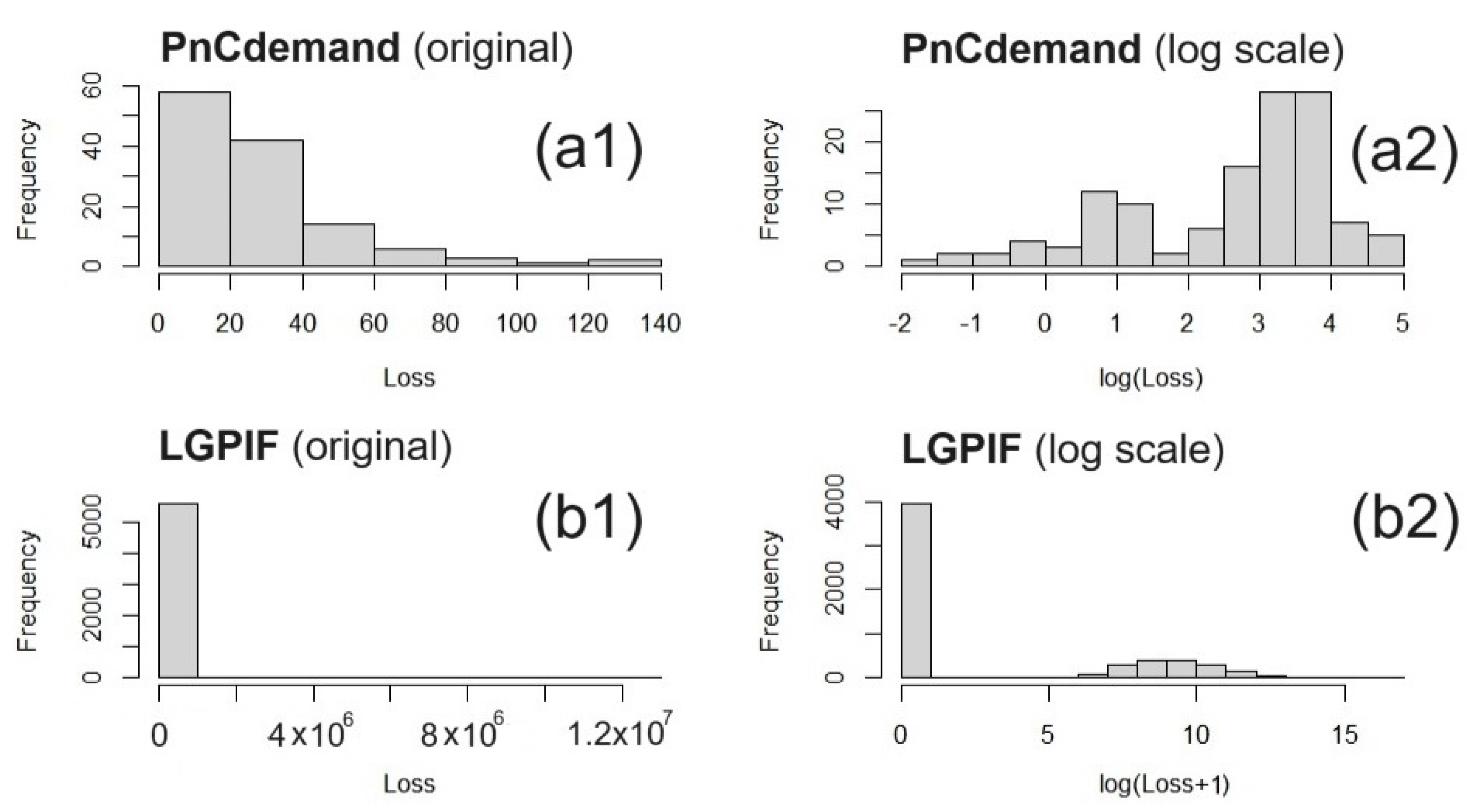
5.1. Data
5.2. Three Competitor Models and Evaluation
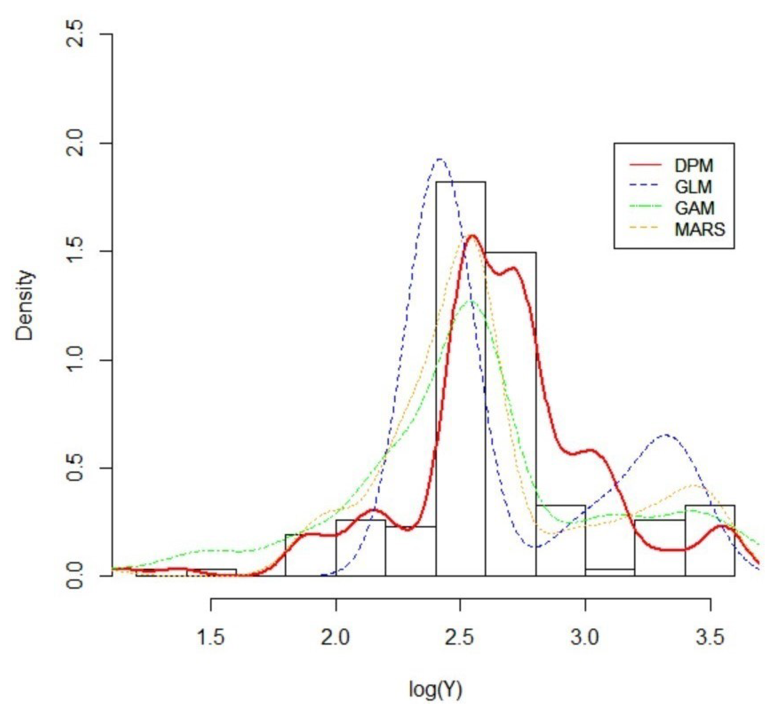
5.3. Result with International General Insurance Liability Data
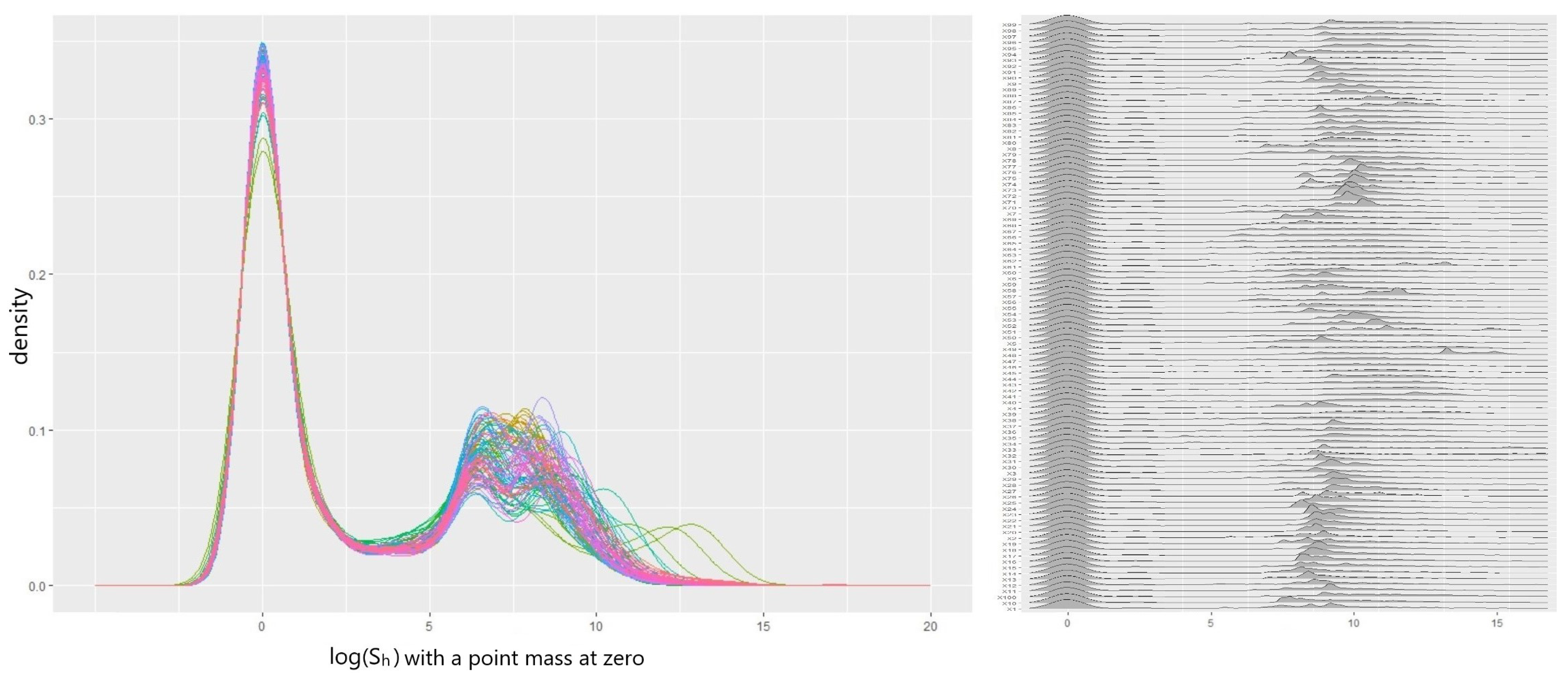
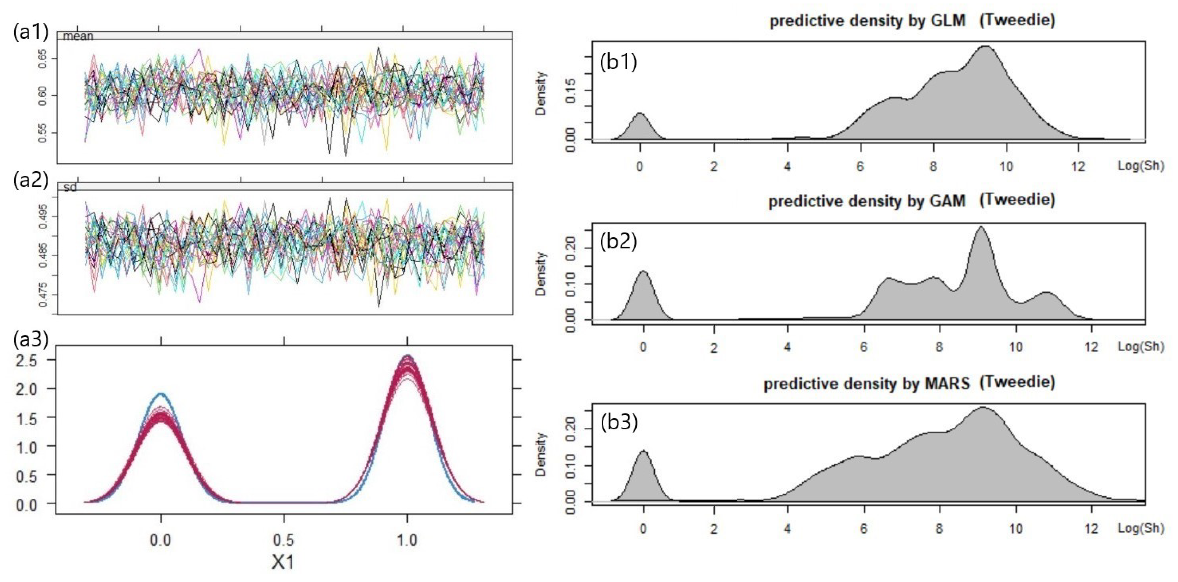
5.4. Result with LGPIF Data
6. Discussion
6.1. Research Questions
6.2. Future Work
- (a)
- Dimensionality: First, in our analysis, we only used two covariates (binary and continuous) for simplicity. Hence, more complex data should be considered. As the number of covariates grows, the likelihood components (covariate models) to describe the covariates grow, which results in the shrinking of the cluster weights. Therefore, using more covariates might enhance the level of sensitivity and accuracy in the creation of cluster memberships. However, it can also introduce more noise or hidden structures that render the resulting predictive distributions unstable. In this sense, further research on the problem of high dimensional covariates in the DPM framework would be worthwhile.
- (b)
- Measurement error: Second, although our focus in this article was the MAR covariate, mismeasured covariates is an equally significant challenge that impairs the proper model development in insurance practice. For example, Aggarwal et al. (2016) pointed out that “model risk” mainly arises due to missingness and measurement error in variables, leading to flawed risk assessments and decision making. Thus, further investigation is necessary to explore the specialized construction of the DPM Gibbs sampler for mismeasured covariates, aiming to prevent the issue of model risk.
- (c)
- Sum of the log skew-normal: Third, as an extension to the approximation of total losses (the sum of individual losses) for a policy, we recommend researching ways to approximate the sum of total losses across entire policies. In other words, we pose the following question: “How do we approximate the sum of log skew-normal random variables?” From the perspective of an executive or an entrepreneur whose concern is the total cash flow of the firm, nothing might be more important than the accurate estimation of the sum of total losses in order to identify the insolvency risk or to make important business decisions.
- (d)
- Scalability: Lastly, we suggest investigating the scalability of the posterior simulation with our DPM Gibbs sampler. As shown in our empirical study on the PnCdemand dataset, our DPM framework produced reliable estimates with relatively small sample sizes (). This was because our DPM framework actively utilized significant prior knowledge in posterior inference rather than heavily relying on the actual features of the data. In the result from the LGPIF dataset, our DPM exhibited stable performance at a sample size as well. However, a sample size of over 10,000 was not explored in this paper. With increasing amounts of data, our DPM framework raises the question of computational efficiency due to the growing demand for computational resources or degradation in performance (see Ni et al. 2020). This is an important consideration, especially in scenarios where the insurance loss information is expected to grow over time.
Author Contributions
Funding
Data Availability Statement
Acknowledgments
Conflicts of Interest
Variable Definitions
| Observation index i in a policy h | |
| Policy index h with a total policy number H | |
| Cluster index for J clusters | |
| Cluster index for observation h | |
| Number of observations in cluster j | |
| Number of observations in cluster j where observation h was removed from | |
| Individual loss i in a policy observation h | |
| Outcome variable which is in a policy observation h. | |
| Outcome variable which is across entire policies | |
| Vector of covariates (including ) for a policy observation h | |
| Vector of covariate (Fire5) | |
| Vector of covariate (Ln(coverage)) | |
| Individual value of covariate (Fire5) for a policy observation h | |
| Individual value of covariate (Ln(coverage)) for a policy observation h | |
| Parameter model (for prior) | |
| Parameter model (for posterior) | |
| Data model (for continuous cluster) | |
| Data model (for discrete cluster) | |
| Logistic sigmoid function—expit(·)—to allow for a positive probability of the zero outcome | |
| Set of parameters——associated with for cluster j | |
| Set of parameters——associated with for cluster j | |
| Cluster weights (mixing coefficient) for cluster j | |
| Vector of initial regression coefficients and variance-covariance matrix (i.e., ) obtained from the baseline multivariate gamma regression of | |
| Regression coefficient vector for a mean outcome estimation | |
| Cluster-wise variation value for the outcome | |
| Skewness parameter for log skew-normal outcome | |
| Vector of initial regression coefficients and variance-covariance matrix obtained from the baseline multivariate logistic regression of | |
| Regression coefficient vector for a logistic function to handle zero outcomes | |
| Proportion parameter for Bernoulli covariate | |
| Location and spread parameter for Gaussian covariate | |
| Precision parameter that controls the variance of the clustering simulation. For instance, a larger allows selecting more clusters. | |
| Prior joint distribution for all parameters in the DPM: , and . It allows all continuous, integrable distributions to be supported while retaining theoretical properties and computational tractability such as asymptotic consistency and efficient posterior estimation. | |
| Hyperparameters for inverse gamma density of | |
| Hyperparameters for Beta density of | |
| Hyperparameters for Student’s t density of | |
| Hyperparameters for Gaussian density of | |
| Hyperparameters for inverse gamma density of | |
| Hyperparameters for gamma density of | |
| Random probability value for gamma mixture density of the posterior on | |
| Mixing coefficient for gamma mixture density of the posterior on |
Appendix A. Parameter Knowledge
Appendix A.1. Prior Kernel for Distributions of Outcome, Covariates, and Precision
Appendix A.2. Posterior Inference for Outcome, Covariates, and Precision
| Algorithm A1 Posterior inference |
|
Appendix B. Baseline Inference Algorithm for the DPM
| Algorithm A2 DPM Gibbs sampling for new cluster development |
|
Appendix C. Development of the Distributional Components for the DPM
Appendix C.1. Derivation of the Distribution of Precision α
- Observation 1 forms a new cluster with a probability =
- Observation 2 forms a new cluster with a probability =
- Observation 3 enters into an existing cluster with a probability =
- Observation 4 enters into an existing cluster with a probability =
- Observation 5 forms a new cluster with a probability =
Appendix C.2. Outcome Data Model of Sh Development with the MAR Covariate x1 for the Discrete Clusters
Appendix C.3. Covariate Data Model of x2 Development with the MAR Covariate x1 for the Continuous Clusters
References
- Aggarwal, Ankur, Michael B. Beck, Matthew Cann, Tim Ford, Dan Georgescu, Nirav Morjaria, Andrew Smith, Yvonne Taylor, Andreas Tsanakas, Louise Witts, and et al. 2016. Model risk–daring to open up the black box. British Actuarial Journal 21: 229–96. [Google Scholar] [CrossRef]
- Antoniak, Charles E. 1974. Mixtures of dirichlet processes with applications to bayesian nonparametric problems. The Annals of Statistics 2: 1152–74. [Google Scholar] [CrossRef]
- Bassetti, Federico, Roberto Casarin, and Fabrizio Leisen. 2014. Beta-product dependent pitman–yor processes for bayesian inference. Journal of Econometrics 180: 49–72. [Google Scholar] [CrossRef]
- Beaulieu, Norman C., and Qiong Xie. 2003. Minimax approximation to lognormal sum distributions. Paper present at the 57th IEEE Semiannual Vehicular Technology Conference, VTC 2003-Spring, Jeju, Republic of Korea, April 22–25; Piscataway: IEEE, vol. 2, pp. 1061–65. [Google Scholar]
- Billio, Monica, Roberto Casarin, and Luca Rossini. 2019. Bayesian nonparametric sparse var models. Journal of Econometrics 212: 97–115. [Google Scholar]
- Blackwell, David, and James B. MacQueen. 1973. Ferguson distributions via pólya urn schemes. The Annals of Statistics 1: 353–55. [Google Scholar] [CrossRef]
- Blei, David M., and Peter I. Frazier. 2011. Distance dependent chinese restaurant processes. Journal of Machine Learning Research 12: 2461–88. [Google Scholar]
- Braun, Michael, Peter S. Fader, Eric T. Bradlow, and Howard Kunreuther. 2006. Modeling the “pseudodeductible” in insurance claims decisions. Management Science 52: 1258–72. [Google Scholar] [CrossRef]
- Browne, Mark J., JaeWook Chung, and Edward W. Frees. 2000. International property-liability insurance consumption. The Journal of Risk and Insurance 67: 73–90. [Google Scholar]
- Cairns, Andrew J. G., David Blake, Kevin Dowd, Guy D. Coughlan, and Marwa Khalaf-Allah. 2011. Bayesian stochastic mortality modelling for two populations. ASTIN Bulletin: The Journal of the IAA 41: 29–59. [Google Scholar]
- Diebolt, Jean, and Christian P. Robert. 1994. Estimation of finite mixture distributions through bayesian sampling. Journal of the Royal Statistical Society: Series B (Methodological) 56: 363–75. [Google Scholar] [CrossRef]
- Escobar, Michael D., and Mike West. 1995. Bayesian density estimation and inference using mixtures. Journal of the American Statistical Association 90: 577–88. [Google Scholar] [CrossRef]
- Ferguson, Thomas S. 1973. A bayesian analysis of some nonparametric problems. The Annals of Statistics 1: 209–30. [Google Scholar] [CrossRef]
- Furman, Edward, Daniel Hackmann, and Alexey Kuznetsov. 2020. On log-normal convolutions: An analytical–numerical method with applications to economic capital determination. Insurance: Mathematics and Economics 90: 120–34. [Google Scholar] [CrossRef]
- Gelman, Andrew, and Jennifer Hill. 2007. Data Analysis Using Regression and Multilevel/Hierarchical Models. Cambridge: Cambridge University Press. [Google Scholar]
- Gershman, Samuel J., and David M. Blei. 2012. A tutorial on bayesian nonparametric models. Journal of Mathematical Psychology 56: 1–12. [Google Scholar] [CrossRef]
- Ghosal, Subhashis. 2010. The dirichlet process, related priors and posterior asymptotics. Bayesian Nonparametrics 28: 35. [Google Scholar]
- Griffin, Jim, and Mark Steel. 2006. Order-based dependent dirichlet processes. Journal of the American statistical Association 101: 179–94. [Google Scholar] [CrossRef]
- Griffin, Jim, and Mark Steel. 2011. Stick-breaking autoregressive processes. Journal of Econometrics 162: 383–96. [Google Scholar] [CrossRef]
- Hannah, Lauren A., David M. Blei, and Warren B. Powell. 2011. Dirichlet process mixtures of generalized linear models. Journal of Machine Learning Research 12: 1923–53. [Google Scholar]
- Hogg, Robert V., and Stuart A. Klugman. 2009. Loss Distributions. Hoboken: John Wiley & Sons. [Google Scholar]
- Hong, Liang, and Ryan Martin. 2017. A flexible bayesian nonparametric model for predicting future insurance claims. North American Actuarial Journal 21: 228–41. [Google Scholar] [CrossRef]
- Hong, Liang, and Ryan Martin. 2018. Dirichlet process mixture models for insurance loss data. Scandinavian Actuarial Journal 2018: 545–54. [Google Scholar] [CrossRef]
- Huang, Yifan, and Shengwang Meng. 2020. A bayesian nonparametric model and its application in insurance loss prediction. Insurance: Mathematics and Economics 93: 84–94. [Google Scholar] [CrossRef]
- Kaas, Rob, Marc Goovaerts, Jan Dhaene, and Michel Denuit. 2008. Modern Actuarial Risk Theory: Using R. Berlin and Heidelberg: Springer Science & Business Media, vol. 128. [Google Scholar]
- Lam, Chong Lai Joshua, and Tho Le-Ngoc. 2007. Log-shifted gamma approximation to lognormal sum distributions. IEEE Transactions on Vehicular Technology 56: 2121–29. [Google Scholar] [CrossRef]
- Li, Xue. 2008. A Novel Accurate Approximation Method of Lognormal Sum Random Variables. Ph.D. thesis, Wright State University, Dayton, OH, USA. [Google Scholar]
- Neal, Radford M. 2000. Markov chain sampling methods for dirichlet process mixture models. Journal of Computational and Graphical Statistics 9: 249–65. [Google Scholar]
- Neuhaus, John M., and Charles E. McCulloch. 2006. Separating between-and within-cluster covariate effects by using conditional and partitioning methods. Journal of the Royal Statistical Society: Series B (Statistical Methodology) 68: 859–72. [Google Scholar] [CrossRef]
- Ni, Yang, Yuan Ji, and Peter Müller. 2020. Consensus monte carlo for random subsets using shared anchors. Journal of Computational and Graphical Statistics 29: 703–14. [Google Scholar] [CrossRef]
- Quan, Zhiyu, and Emiliano A. Valdez. 2018. Predictive analytics of insurance claims using multivariate decision trees. Dependence Modeling 6: 377–407. [Google Scholar] [CrossRef]
- Richardson, Robert, and Brian Hartman. 2018. Bayesian nonparametric regression models for modeling and predicting healthcare claims. Insurance: Mathematics and Economics 83: 1–8. [Google Scholar] [CrossRef]
- Rodriguez, Abel, and David B. Dunson. 2011. Nonparametric bayesian models through probit stick-breaking processes. Bayesian Analysis (Online) 6: 145–78. [Google Scholar]
- Roy, Jason, Kirsten J. Lum, Bret Zeldow, Jordan D. Dworkin, Vincent Lo Re III, and Michael J. Daniels. 2018. Bayesian nonparametric generative models for causal inference with missing at random covariates. Biometrics 74: 1193–202. [Google Scholar] [CrossRef]
- Sethuraman, Jayaram. 1994. A constructive definition of dirichlet priors. Statistica Sinica 4: 639–650. [Google Scholar]
- Shah, Anoop D., Jonathan W. Bartlett, James Carpenter, Owen Nicholas, and Harry Hemingway. 2014. Comparison of random forest and parametric imputation models for imputing missing data using mice: A caliber study. American Journal of Epidemiology 179: 764–74. [Google Scholar] [CrossRef] [PubMed]
- Shahbaba, Babak, and Radford Neal. 2009. Nonlinear models using dirichlet process mixtures. Journal of Machine Learning Research 10: 1829–50. [Google Scholar]
- Shams Esfand Abadi, Mostafa. 2022. Bayesian Nonparametric Regression Models for Insurance Claims Frequency and Severity. Ph.D. thesis, University of Nevada, Las Vegas, NV, USA. [Google Scholar]
- Si, Yajuan, and Jerome P. Reiter. 2013. Nonparametric bayesian multiple imputation for incomplete categorical variables in large-scale assessment surveys. Journal of Educational and Behavioral Statistics 38: 499–521. [Google Scholar] [CrossRef]
- Suwandani, Ria Novita, and Yogo Purwono. 2021. Implementation of gaussian process regression in estimating motor vehicle insurance claims reserves. Journal of Asian Multicultural Research for Economy and Management Study 2: 38–48. [Google Scholar] [CrossRef]
- Teh, Yee Whye. 2010. Dirichlet Process. In Encyclopedia of Machine Learning. Berlin and Heidelberg: Springer Science & Business Media, pp. 280–87. [Google Scholar]
- Ungolo, Francesco, Torsten Kleinow, and Angus S. Macdonald. 2020. A hierarchical model for the joint mortality analysis of pension scheme data with missing covariates. Insurance: Mathematics and Economics 91: 68–84. [Google Scholar] [CrossRef]
- Zhao, Lian, and Jiu Ding. 2007. Least squares approximations to lognormal sum distributions. IEEE Transactions on Vehicular Technology 56: 991–97. [Google Scholar] [CrossRef]


| Model | AIC | SSPE | SAPE | 10% CTE | 50% CTE | 90% CTE | 95% CTE |
|---|---|---|---|---|---|---|---|
| Ga-GLM | 830.56 | 268.6 | 139.8 | 6.5 | 13.8 | 54.5 | 78.0 |
| Ga-MARS | 830.58 | 267.2 | 138.2 | 6.1 | 13.0 | 57.2 | 71.1 |
| Ga-GAM | 845.94 | 266.7 | 136.1 | 6.2 | 13.3 | 58.1 | 72.2 |
| LogN-DPM | - | 272.0 | 134.7 | 6.4 | 13.8 | 59.3 | 79.3 |
| Model | AIC | SSPE | SAPE | 10% CTE | 50% CTE | 90% CTE | 95% CTE |
|---|---|---|---|---|---|---|---|
| Tweedie-GLM | 26,270.3 | 2.04 × 10 | 89,380,707 | 955.9 | 12,977.2 | 133,374.4 | 340,713.1 |
| Tweedie-MARS | 24,721.4 | 1.99 × 10 | 88,594,850 | 961.7 | 10,391.0 | 129,409.2 | 355,112.6 |
| Tweedie-GAM | 21,948.9 | 1.95 × 10 | 88,213,987 | 989.4 | 13,026.2 | 140,199.5 | 398,263.1 |
| LogSN-DPM | - | 1.98 × 10 | 83,864,890 | 975.3 | 13,695.1 | 147,486.6 | 425,682.6 |
Disclaimer/Publisher’s Note: The statements, opinions and data contained in all publications are solely those of the individual author(s) and contributor(s) and not of MDPI and/or the editor(s). MDPI and/or the editor(s) disclaim responsibility for any injury to people or property resulting from any ideas, methods, instructions or products referred to in the content. |
© 2023 by the authors. Licensee MDPI, Basel, Switzerland. This article is an open access article distributed under the terms and conditions of the Creative Commons Attribution (CC BY) license (https://creativecommons.org/licenses/by/4.0/).
Share and Cite
Kim, M.; Lindberg, D.; Crane, M.; Bezbradica, M. Dirichlet Process Log Skew-Normal Mixture with a Missing-at-Random-Covariate in Insurance Claim Analysis. Econometrics 2023, 11, 24. https://doi.org/10.3390/econometrics11040024
Kim M, Lindberg D, Crane M, Bezbradica M. Dirichlet Process Log Skew-Normal Mixture with a Missing-at-Random-Covariate in Insurance Claim Analysis. Econometrics. 2023; 11(4):24. https://doi.org/10.3390/econometrics11040024
Chicago/Turabian StyleKim, Minkun, David Lindberg, Martin Crane, and Marija Bezbradica. 2023. "Dirichlet Process Log Skew-Normal Mixture with a Missing-at-Random-Covariate in Insurance Claim Analysis" Econometrics 11, no. 4: 24. https://doi.org/10.3390/econometrics11040024