Article

Multistep Forecast Averaging with Stochastic and Deterministic Trends

1
Daniels School of Business, Purdue University, 403 Mitch Daniels Blvd., West Lafayette, IN 47907, USA
2
Department of Applied Economics, School of Management, Fudan University, 670 Guoshun Road, Shanghai 200433, China
*
Author to whom correspondence should be addressed.
Econometrics 2023, 11(4), 28; https://doi.org/10.3390/econometrics11040028
Submission received: 24 August 2023 / Revised: 27 November 2023 / Accepted: 7 December 2023 / Published: 15 December 2023

Abstract

:
This paper presents a new approach to constructing multistep combination forecasts in a nonstationary framework with stochastic and deterministic trends. Existing forecast combination approaches in the stationary setup typically target the in-sample asymptotic mean squared error (AMSE), relying on its approximate equivalence with the asymptotic forecast risk (AFR). Such equivalence, however, breaks down in a nonstationary setup. This paper develops combination forecasts based on minimizing an accumulated prediction errors (APE) criterion that directly targets the AFR and remains valid whether the time series is stationary or not. We show that the performance of APE-weighted forecasts is close to that of the optimal, infeasible combination forecasts. Simulation experiments are used to demonstrate the finite sample efficacy of the proposed procedure relative to Mallows/Cross-Validation weighting that target the AMSE as well as underscore the importance of accounting for both persistence and lag order uncertainty. An application to forecasting US macroeconomic time series confirms the simulation findings and illustrates the benefits of employing the APE criterion for real as well as nominal variables at both short and long horizons. A practical implication of our analysis is that the degree of persistence can play an important role in the choice of combination weights.

1. Introduction

The pioneering work of Granger (1966) demonstrated that a large number of macroeconomic time series have a typical spectral shape dominated by a peak at low frequencies. This finding suggests the presence of relatively long run information in the current level of the variables, which should be taken into account when modeling their time series evolution and can potentially be exploited to yield improved forecasts. One way to incorporate this long-run information in econometric modeling is through stochastic trends (unit roots) and/or deterministic trends. However, given that trends are slowly evolving, there is only limited information in any data set about how best to specify the trend or distinguish between alternative models of the trend. For instance, unit root tests often fail to reject a unit root despite the fact that theory does not postulate the presence of a unit root for many macroeconomic variables [see Elliott (2006), for further discussion of this issue]. Therefore, it appears prudent to incorporate the uncertainty arising from the presence of a stochastic trend when constructing macroeconomic forecasts. Moreover, this uncertainty is likely to be particularly important for longer horizons.1
A second source of uncertainty involved in the construction of forecasts relates to the specification of short-run dynamics driving the time series. Within an autoregressive modeling framework, this form of uncertainty can be expressed in terms of the lags of first differences of the time series being analyzed. Since the number of lags that ought to be included in the model is unknown in practice, there is a bias–variance trade-off facing the forecaster: underspecifying the number of lags would lead to biased forecasts, while including irrelevant lags would induce a higher forecast variance. The challenge therefore lies in incorporating lag order uncertainty in a manner that best addresses this trade-off.
Motivated by these considerations, this paper proposes a new multistep forecast combination approach designed for forecasting a highly persistent time series that simultaneously addresses uncertainty about the presence of a stochastic trend and uncertainty about the nature of short-run dynamics within a unified autoregressive modeling framework. Unlike extant forecast combination approaches, we develop combination forecasts based on minimizing the so-called accumulated prediction errors (APE) criterion that directly targets the asymptotic forecast risk (AFR) instead of the in-sample asymptotic mean squared error (AMSE). This is particularly relevant, since the equivalence between AFR and AMSE breaks down in a nonstationary setup. Our analysis generalizes existing results by establishing the asymptotic validity of the APE for multistep forecasts in the unit root and (fixed) stationary cases, both for models with and without deterministic trends. We further show that, regardless of the presence of a unit root, the performance of APE-weighted forecasts remains close to that of the infeasible combination forecasts which assume that the optimal (i.e., AFR minimizing) weights are known. Monte Carlo experiments are used to (i) demonstrate the finite sample efficacy of the proposed procedure relative to Mallows/Cross-Validation weighting that target the AMSE; (ii) underscore the importance of accounting for uncertainty about the stochastic trend and/or the lag order. In a pseudo out-of-sample forecasting exercise applied to US monthly macroeconomic time series, we evaluate the performance of a variety of selection/combination-based approaches at horizons of one, three, six, and twelve months. Consistent with the simulation results, the empirical analysis provides strong evidence in favor of a version of the advocated approach that simultaneously addresses stochastic trend and lag order uncertainty regardless of the forecast horizon considered.
The present study builds on previous work by Hansen (2010a) and Kejriwal and Yu (2021) who analyzed one-step ahead combination forecasts allowing for both persistence and lag order uncertainty. In particular, Hansen (2010a) adopted a local-to-unity framework to develop combination forecasts that combine forecasts from the restricted (i.e., imposing a unit root) and unrestricted models with the weights obtained by minimizing a one-step Mallows criterion. To address lag order uncertainty, he also proposed a general combination approach that, in addition to the restricted and unrestricted model forecasts, also combines forecasts based on different lag orders. Kejriwal and Yu (2021) provided theoretical justification for the general combination approach and developed improved combination forecasts that employ feasible generalized least squares (FGLS) estimates instead of ordinary least squares (OLS) estimates of the deterministic trend component.
Our paper can be viewed as extending Hansen’s (2010a) approach in two practically relevant directions. First, in addition to one-step ahead forecasts, we also analyze the statistical properties of multistep combination forecasts given that uncertainty regarding the presence of a stochastic trend is especially relevant over longer horizons. Second, in contrast to Mallows weighting as advocated by Hansen (2010a), our combination weights are obtained via the APE criterion that directly targets the AFR instead of the AMSE. Our Monte Carlo and empirical comparisons of the performance of combination forecasts based on different weighting schemes clearly illustrate the importance of directly targeting the AFR. Thus, an important implication of our study is that the preferred choice of weighting scheme when combining forecasts can critically depend on whether the variables involved are stationary or not.
The recent machine learning literature has proposed a variety of forecasting methods that exploit information in a large number of potential predictors (see, e.g., Masini et al. 2023, for a survey). In contrast, our study is univariate in that it only utilizes past information about the variable of interest to develop forecasts. A natural question one may ask, then, is what is the value added by our univariate forecasting approach when more sophisticated machine learning approaches are available? We offer three possible responses. First, our approach is simple to use in practice, since it only requires running OLS regressions. Second, it is transparent in that its statistical properties can be studied analytically, which can be useful for understanding the merits and limitations of the approach. Third, when evaluating the performance of machine learning methods, our preferred forecasting approach can provide a much more competitive univariate benchmark for comparison than a simple autoregressive model with a prespecified/estimated lag order which has routinely been used as the benchmark (see, e.g., Kim and Swanson 2018; Medeiros et al. 2021).
The rest of the paper is organized as follows. Section 2 provides a review of the related literature. Section 3 presents the model and the related estimators. Section 4 analyzes the AMSE and AFR as alternative measures of forecast accuracy. Section 5 discusses the choice of combination weights based on the APE criterion. Section 6 extends the analysis to allow for lag order uncertainty in the construction of the forecasts. Monte Carlo evidence, including comparisons with various existing methods, is provided in Section 7. Section 8 details an empirical application to forecasting US macroeconomic time series and Section 9 concludes. Appendix A, Appendix B and Appendix C contain, respectively, the proofs, details of forecasting methods considered, and additional simulation results. All computations were carried out in the 2022b version of MATLAB (2022).

2. Literature Review

A common practice in the economic forecasting literature is to apply a stationarity-inducing transformation (e.g., differencing or detrending) to the time series of interest and then attempt to forecast the transformed series. Consequently, most of the forecasting procedures in current use have been developed under the assumption of data stationarity. The traditional approach of Box and Jenkins (1970) transforms the data through differencing which amounts to modeling the low-frequency peak in the spectrum as a zero-frequency phenomenon and proceeds to forecast the transformed series using standard stationary autoregressive moving average (ARMA) models. More recently, Stock and Watson (2005, 2006) constructed a extensive database of 132 monthly macroeconomic time series over the period 1959-2003 and applied a variety of transformations to render them stationary before using a handful of common factors extracted from the data set using principal components as predictors (the so-called diffusion-index methodology). Similarly, McCracken and Ng (2016) assembled a publicly available database of 134 monthly time series referred to as FRED-MD and updated on a timely basis by the Federal Reserve Bank of St Louis. They also suggested a set of data transformations which is used to construct factor-based diffusion indexes for forecasting as well as to analyze business cycle turning points.
While convenient in practice, the approach of forecasting the transformed stationary series tends to ignore the information in the levels of the variables. In particular, it does not properly account for the uncertainty arising from the nature of the underlying trends, which can lead to poor forecasts if the trends are misspecified. Clements and Hendry (2001) documented, both analytically and numerically, the detrimental consequences of trend misspecification on the resulting forecasts in the presence of parameter estimation uncertainty. Specifically, they found that when the sample size increases at a faster rate than the forecast horizon, misspecifying a difference stationary process as trend stationary or vice versa yields forecast error variances of a higher order of magnitude relative to the correctly specified model. Consequently, the objective of our study is to construct forecasts of the time series in levels and explicitly model the uncertainty regarding the presence of a stochastic trend instead of transforming the time series to stationarity based on a trend specification that is determined a priori and is possibly misspecified.
Our study is closely related to the existing literature on methods for forecasting nonstationary time series. Diebold and Kilian (2000) showed that a unit root pretesting strategy can improve forecast accuracy relative to restricted or unrestricted estimation. Ng and Vogelsang (2002) found that the use of FGLS estimates of the trend component can yield superior forecasts relative to their OLS counterparts. Turner (2004) recommended the use of forecasting thresholds whereby the restricted (unit root) forecast is preferred on one side of these thresholds while the unrestricted (OLS) forecast is preferred on the other. His proposal was based on median unbiased estimation of the local-to-unity parameter to determine the thresholds and was shown to dominate a unit root pretesting strategy. Ing et al. (2012) studied the impact of nonstationarity, model complexity and model misspecification on the AFR in infinite order autoregressions.
A promising approach to addressing both stochastic trend uncertainty and lag order uncertainty is forecast combination. Introduced in the seminal work of Bates and Granger (1969), the idea underlying forecast combination is to exploit the bias–variance trade-off by combining forecasts from restricted (possibly subject to bias) specifications and unrestricted (possibly subject to overfitting) specifications using an appropriate choice of combination weights. A voluminous amount of literature has subsequently developed, which has analyzed the efficacy of several alternative weighting schemes for constructing the combination forecasts (see, e.g.,Wang et al. 2022, for a recent survey). Hansen (2010a) proposed one-step ahead combination forecasts within an autoregressive modeling framework that accounts for both aforementioned sources of uncertainty, where the combination weights are obtained by minimizing a Mallows criterion. The Mallows criterion is designed to provide an approximately unbiased estimator of the in-sample AMSE. Hansen’s analysis showed that the unit root pretesting strategy could be subject to high forecast risk for a range of persistence levels, while his combination forecast performed favorably compared to a number of methods popular in applied work and dominated the unrestricted forecast uniformly in terms of finite sample forecast risk. Kejriwal and Yu (2021) proposed a refinement of Hansen’s (2010a) approach, which entails estimating the deterministic trend component by FGLS instead of OLS. Tu and Yi 2017 analyzed one-step forecasting based on the Mallows averaging estimator in a cointegrated vector autoregressive model and found that it dominated the commonly used approach of pretesting for cointegration.
In a stationary setup, combination forecasts based on Mallows/cross-validation (CV) weighting typically target the AMSE, relying on its approximate equivalence with the AFR (e.g., Hansen 2008, 2010b; Liao and Tsay 2020). Such equivalence, however, breaks down in a nonstationary setup. Hansen (2010a) showed, within a local-to-unity framework, that the AMSEs of unrestricted as well as restricted (imposing a unit root) one-step ahead forecasts are different from the corresponding expressions for their AFR in autoregressive models (see Section 4 for further discussion on the issue of equivalence or lack thereof).
To address the lack of equivalence between AMSE and AFR, we develop combination forecasts based on minimizing the APE criterion that directly targets the AFR instead of the AMSE. Previous work in the context of model selection has shown the APE criterion to remain valid whether the process is stationary or has a unit root. Specifically, Ing (2004) showed that a normalized version of the APE is almost certain to the AFR in the stationary case, while a similar result was obtained by Ing et al. (2009) in the unit root case. Focusing on the first-order autoregressive case and one-step ahead forecasts, Yu et al. (2012) extended the validity of the APE to a unit root model with a deterministic time trend. Our study extends the use of the APE criterion to construct combination forecasts in a nonstationary environment.
In summary, there is a plethora of approaches available in the literature for forecasting nonstationary time series, including model selection, pretesting, and forecast combination. Combination forecasts have often been shown to incur lower forecast risk in practice than forecasts based on model selection or pretesting. However, the existing literature has typically employed weighting schemes such as Mallows/CV weighting that have been formally justified only in a stationary framework. Our study contributes to this literature by demonstrating that when the variable of interest is potentially nonstationary, it may be desirable to construct the combination weights using an alternative approach (the APE criterion). Our findings are particularly relevant for macroeconomic applications, given that several macroeconomic time series have been documented to exhibit a degree of persistence that is difficult to distinguish from a unit root process.

3. Model and Estimation

We consider a univariate time series y t   generated as follows:
y t = m t + u t m t = β 0 + β 1 t + + β p t p u t = α u t 1 + α 1 Δ u t 1 + + α k Δ u t k + e t α = 1 + a c T ,         a = 1 α 1 α k ,       c 0
where p { 0 , 1 } is the order of the trend component and the stochastic component u t   follows a finite order autoregressive process of order ( k + 1 ) process driven by the innovations e t . The uncertainty about the stochastic trend is captured by the persistence parameter α   that is modeled as local-to-unity with c = 0   corresponding to the unit root case and c < 0   to the stationary case. The initial observations are set at u 0 , u 1 , , u k = O p ( 1 ) .2 This section treats the true lag order k   as known. Lag order uncertainty is addressed in Section 6. Our analysis is based on the following assumptions:
Assumption 1.
The sequence { e t }   is a martingale difference sequence with E ( e t | F t 1 ) = 0   and E ( e t 2 | F t 1 ) = σ 2 ,   where 0 < σ 2 < ,   and F t   is the σ-field generated by { e s ;   s t } . Moreover, there exist small positive numbers ϕ 1   and ϕ 2   and a large positive number M 1   , such that for 0 s s ϕ 2 ,
sup 1 m t < ,   v m = 1 F t , m , v m ( s ) F t , m , v m ( s ) M 1 ( s s ) ϕ 1 ,
where v m = ( v 1 , , v m ) R m ,   v m = j = 1 m v j 2   and F t , m , v m ( . )   denotes the distribution of l = 1 m v l e t + 1 l .
Assumption 2.
All roots of A ( L ) = 1 i = 1 k α i L i   lie outside the unit circle.
The data generating process in (1) and Assumptions 1 and 2 are adopted from Hansen (2010a) with an additional restriction on the distribution of { e t } , which ensures that the sample second moments of the regressors are bounded in expectation (see Ing et al. 2009). The difference between our modeling framework and Ing et al. (2009) is that they impose an exact unit root ( c = 0 ), while we allow c 0 . For h 1 , let the optimal (infeasible) mean squared error minimizing h-step ahead forecast of y t   be denoted as μ t + h . It is the conditional mean of y t + h   given F t , which is obtained from the following recursion (Hamilton 1994, pp. 80–82):
μ t + h = z t + h β + α ( μ t + h 1 z t + h 1 β ) + α 1 ( Δ μ t + h 1 Δ z t + h 1 β )       + + α k ( Δ μ t + h k Δ z t + h k β )
with μ t + j = y t + j if j 0 ;   β = β 0 and z t = 1 if   p = 0   ;   β = ( β 0 , β 1 ) and z t = ( 1 , t ) if p = 1 . We can further rewrite (2) as
μ t + h = z t + h β * + α μ t + h 1 + j = 1 k α j Δ μ t + h j
where β * = ( 1 α ) β 0   if z t = 1   and β * = ( β 0 * , β 1 * )   with β 0 * = ( 1 α ) β 0 + ( α j = 1 k α j ) β 1 , β 1 * = ( 1 α ) β 1   if z t = ( 1 , t ) .
We consider three alternative estimators of μ t + h . The first is the unrestricted estimator μ ^ t + h obtained as
μ ^ t + h = z t + h β ^ * + α ^ μ ^ t + h 1 + j = 1 k α ^ j Δ μ ^ t + h j
with μ ^ t + j = y t + j   if j 0   where ( β ^ * , α ^ , α ^ j )   are the OLS estimates from the regression
y s = z s β * + α y s 1 + j = 1 k α j Δ y s j + e s ,       s = k + 2 , , T
Instead of using ( 4 ) ,   one may consider a two-step strategy for estimating μ t + h   that entails regressing y t   on z t   and obtaining the estimate β ^   of β and the residuals u ^ t = y t z t β ^   in a first step and then estimating an autoregression of order k + 1   in u ^ t   to obtain the estimates of ( α , α 1 , , α k ) . The forecasts are obtained from ( 4 ) . However, as shown in Ng and Vogelsang (2002), the one-step estimate μ ^ t + h   is preferable to the two-step estimate with persistent data.
The second estimator is the restricted estimator μ ˜ t + h   that imposes the unit root restriction α = 1   and is obtained as
μ ˜ t + h = Δ z t + h β ˜ * + μ ˜ t + h 1 + j = 1 k α ˜ j Δ μ ˜ t + h j
with μ ˜ t + j = y t + j   if j 0   where ( β ˜ * , α ˜ , α ˜ j )   are the OLS estimates from the regression
Δ y s = Δ z s β * + j = 1 k α j Δ y s j + e s ,       s = k + 2 , , T
Finally, the third estimator is based on taking a weighted average of the unrestricted and restricted forecasts. Letting w [ 0 , 1 ]   be the weight assigned to the unrestricted estimator, the averaging estimator is given by
μ ^ t + h ( w ) = w μ ^ t + h + ( 1 w ) μ ˜ t + h
The relative accuracy of the three foregoing estimators can be evaluated using the asymptotic forecast risk (AFR), which is the limit of the h-step ahead expected squared forecast error:
f 0 ( c , p , k , h ) = lim T T σ 2 E ( μ ˜ T + h μ T + h ) 2 f 1 ( c , p , k , h ) = lim T T σ 2 E ( μ ^ T + h μ T + h ) 2 f w ( c , p , k , h ) = lim T T σ 2 E ( μ ^ T + h ( w ) μ T + h ) 2
In order to derive analytical expressions for the AFR, we introduce the following notation. Let W ( . ) denote a standard Brownian motion on [ 0 , 1 ] and define the Ornstein–Uhlenbeck process
d W c ( r ) = c W c ( r ) + d W ( r )
For p { 0 , 1 } ,   let X c ( r ) = ( r p , W c ( r ) )   and define the stochastic processes
W c * ( r , p ) = W c ( r ) W c ( r ) 0 1 W c ( s ) d s if if p = 0 p = 1 X c * ( r , p ) = X c ( r ) X c ( r ) 0 1 X c ( s ) d s if if p = 0 p = 1
and the functionals
T 0 c = c W c * ( 1 , p ) + I ( p = 1 ) W ( 1 ) T 1 c = X c * ( 1 , p ) 0 1 X c * ( r , p ) X c * ( r , p ) 1 0 1 X c * ( r , p ) d W ( r ) + I ( p = 1 ) W ( 1 )
Next, note that from ( 1 ) , we can write
y t + h = E t ( y t + h ) + η t , h
where η t , h = j = 0 h 1 b j e t + h j ,   E t ( . )   denotes conditional expectation with respect to information at time t   and the coefficients b j   ( j = 0 , , h 1 )   are obtained by equating coefficients of L j   on both sides of the equation
b ( L ) d ( L ) = 1
where b ( L ) = j = 0 h 1 b j L j   and d ( L ) = 1 α L ( 1 L ) j = 1 k α j L j . When α = 1 ,   b j = i = 0 j ν i ,   ν 0 = 1   and ν j ;   j 1 ,   satisfies 1 + j = 1 ν j L j = 1 / A ( L ) (see Ing et al. 2009).
Denoting α ( k ) = ( α 1 , , α k ) ,   we define the following quantities:
S M ( k ) = α ( k 1 ) I k 1 α k 0 k 1     ,     S M 0 ( k ) = I k M h ( k ) = j = 0 h 1 b j S M h 1 j ( k ) ,     Γ ( k ) = lim j E ( s j ( k ) s j ( k ) ) ,     s j ( k ) = ( Δ y j , , Δ y j k + 1 ) g h ( k ) = 0 t r Γ ( k ) M h ( k ) Γ 1 ( k ) M h ( k ) if k = 0 if k 1
With the above notation in place, we obtain the following result, which provides an analytical representation for the AFR of the unrestricted and restricted forecasts:
Theorem 1.
Under Assumptions 1 and 2 and sup t   E ( e t θ h ) < ,   where θ h = max { 8 ,   2 ( h + 2 ) } + ψ   for some ψ > 0 ,
(a) f 1 ( c , p , k , h ) = f 1 ( c , p , h ) + g h ( k ) ,   f 1 ( c , p , h ) = j = 0 h 1 b j 2 E ( T 1 c 2 ) .
(b) f 0 ( c , p , k , h ) = f 0 ( c , p , h ) + g h ( k ) ,   f 0 ( c , p , h ) = j = 0 h 1 b j 2 E ( T 0 c 2 ) .
Theorem 1 shows that the AFR of both the restricted and unrestricted forecasts can be decomposed into two components: the first component f j ( c , p , h ) ,   j = 0 , 1 ,   depends on both the underlying stochastic/deterministic trends as well as the short-run dynamics through the coefficients { b j } ;   the second component g h ( k )   is common to the restricted and unrestricted estimators and depends on the parameters governing the short-run dynamics of the time series. The result generalizes Theorem 2 of Hansen (2010a) for one-step forecasts to multistep forecasts. Interestingly, when h = 1 , the AFR can be expressed as the sum of a purely nonstationary component representing the stochastic/deterministic trends (since b 0 = 1 ) and a stationary short-run component which is simply the number of first-differenced lags, i.e., g 1 ( k ) = k . However, as Theorem 1 shows, when h > 1 ,   such a stationary-nonstationary decomposition no longer holds, since both components now depend on the short-run coefficients { α j } . Theorem 1 also generalizes Theorem 2.2 of Ing et al. (2009), which derived an expression for AFR assuming an exact unit root ( c = 0 ) and no deterministic component.
The next result, which follows as a direct consequence of Theorem 1, shows that the optimal combination weight is independent of the forecast horizon and the moving average coefficients { b j }   but depends on the nuisance parameter c:
Corollary 1.
The AFR of the combination forecast is given by
f w ( c , p , k , h ) = j = 0 h 1 b j 2 w 2 E ( T 1 c 2 ) + ( 1 w ) 2 E ( T 0 c 2 ) + 2 w ( 1 w ) E ( T 1 c T 0 c ) + g h ( k )
with optimal (i.e., AFR minimizing) weight
w * = E ( T 0 c 2 ) E ( T 0 c T 1 c ) E ( T 0 c 2 ) + E ( T 1 c 2 ) 2 E ( T 0 c T 1 c )

4. Asymptotic Mean Squared Error and Asymptotic Forecast Risk

An alternative measure of forecast accuracy is the in-sample asymptotic mean squared error (AMSE) defined as
m u ( c , p , k , h ) = lim T 1 σ 2 t = 1 T h E ( μ ^ t + h μ t + h ) 2
for the unrestricted estimator with similar expressions in place for the restricted and averaging estimators. Hansen (2008) established the approximate equivalence between this measure and the AFR under the assumption of strict stationarity. Accordingly, existing forecast combination approaches developed in the stationary framework are based on targeting the AMSE by appealing to its equivalence with the AFR. Hansen (2008) proposed estimating the weights by minimizing a Mallows (2000) criterion which yields an asymptotically unbiased estimate of the AMSE. Similarly, Hansen (2010b) demonstrated that a leave-h-out cross validation criterion delivers an asymptotically unbiased estimate of the AMSE.
This equivalence result, however, breaks down in a nonstationary setup. For instance, when the process has a unit root with no drift and the regression does not include a deterministic component, it follows from the results in Hansen (2010a) that the AMSE of the one-step ahead forecast coincides with the expected value of the squared limiting Dickey–Fuller t-statistic. This expectation has been shown to be about 1.141 by Gonzalo and Pitarakis (1998) and Meng (2005) using analytical and numerical integration techniques, respectively. In contrast, Ing (2001) theoretically established that the AFR of the one-step ahead forecast for the same data generating process and regression is two. More recently, Hansen (2010a) demonstrated the lack of equivalence within a local-to-unity framework, showing that the AMSE of unrestricted as well as restricted (imposing a unit root) one-step ahead forecasts are different from the corresponding expressions for their AFR in autoregressive models with a general lag order and a deterministically trending component. Notwithstanding this result, he suggested using a Mallows criterion to estimate the combination weights and evaluated the adequacy of the resulting combination forecast in finite samples via simulations. A similar approach was taken by Kejriwal and Yu (2021), who also employed Mallows weighting but estimated the deterministic component by FGLS in order to improve upon the accuracy of OLS-based forecasts.
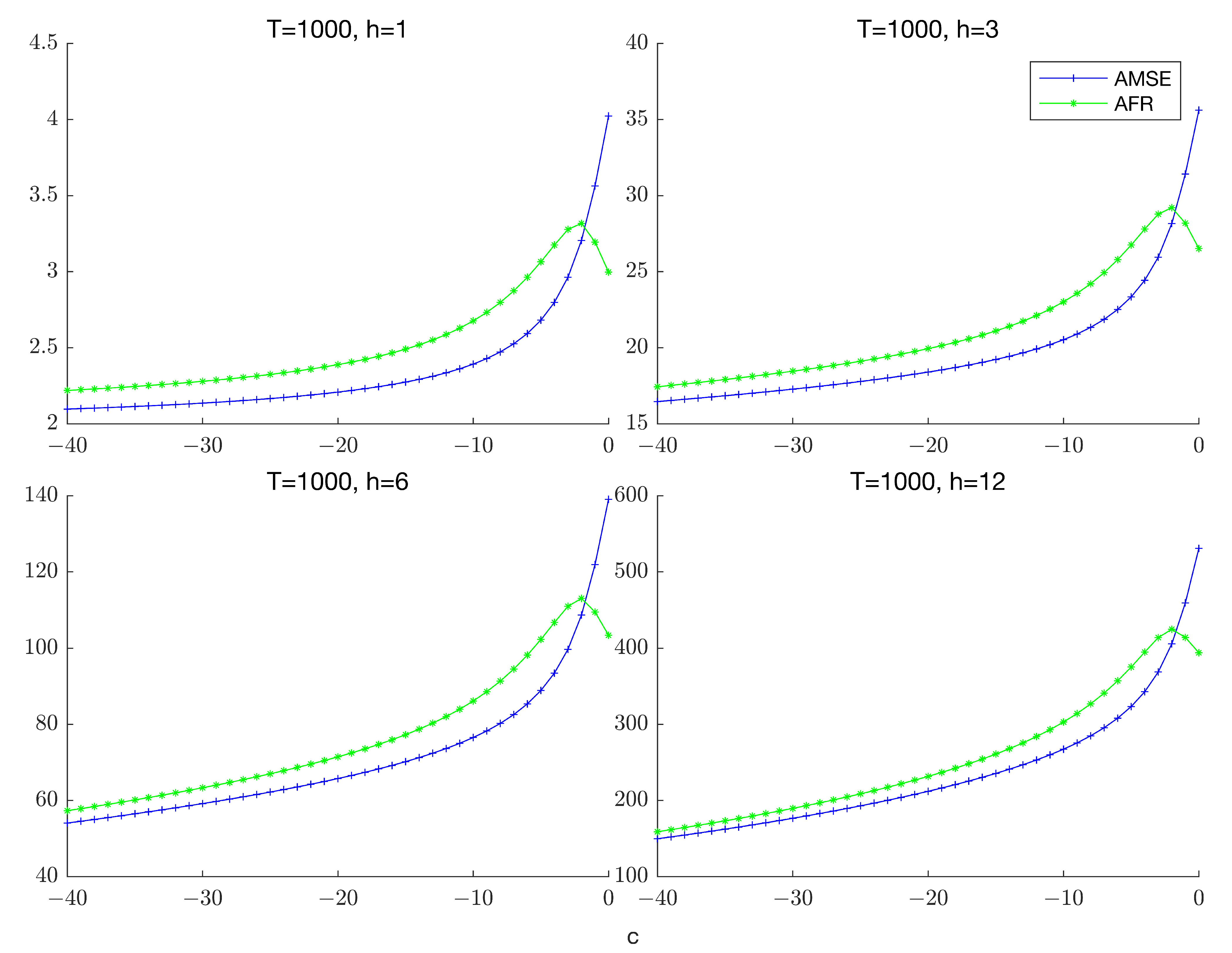
To illustrate the failure of equivalence, Figure 1 plots the AMSE and the AFR of the unrestricted estimator for the case p = 0 and k = 0 .3 The figure clearly illustrates that while the two measures of forecast accuracy follow a similar path for c sufficiently far from zero, they tend to diverge as the process becomes more persistent. This pattern remains robust across different forecast horizons and suggests that a forecast combination approach that directly targets AFR instead of AMSE can potentially generate more accurate forecasts of highly persistent time series when forecast risk is used as a metric for forecast evaluation.

5. Choice of Combination Weights

The optimal combination forecast μ ^ t + h ( w * ) is infeasible in practice, since the weight w * depends on the unknown local-to-unity parameter c   that is not consistently estimable. Given the lack of equivalence between AMSE and AFR for nonstationary time series as discussed in the previous section, we pursue an alternative approach to estimating the combination weights that directly targets the AFR, which is a more direct and practical measure of forecast accuracy than AMSE. In particular, the estimated weight w ^ is obtained by minimizing the so-called accumulated prediction errors (APE) criterion defined as
A P E ( w ) = i = m h T h y i + h μ ^ i + h ( w ) 2 = i = m h T h w ( y i + h μ ^ i + h ) + ( 1 w ) ( y i + h μ ˜ i + h ) 2
with respect to w ,   where w [ 0 , 1 ] ,   μ ^ i + h ( w )   is the h-step ahead combination forecast based only on data up to period i, and m h   denotes the smallest positive number such that the forecasts μ ^ i + h   and μ ˜ i + h   are well defined for all i m h . The solution is given by
w ^ = i = m h T h ( y i + h μ ˜ i + h ) 2 i = m h T h ( y i + h μ ^ i + h ) ( y i + h μ ˜ i + h ) i = m h T h ( y i + h μ ˜ i + h ) 2 + i = m h T h ( y i + h μ ^ i + h ) 2 2 i = m h T h ( y i + h μ ^ i + h ) ( y i + h μ ˜ i + h )
The APE criterion with h = 1 was first introduced by Rissanen (1986) in the context of model selection. Wei (1987) derived the asymptotic properties of APE in general regression models and specialized his results to stationary and nonstationary autoregressive processes with h = 1 . Ing (2004) demonstrated the strong consistency of the APE-based lag order estimator in stationary autoregressive models for h 1 . In particular, he showed that a normalized version of the APE is almost certain to converge to the AFR in large samples. Ing et al. (2009) extended the analysis to autoregressive processes with a unit root. The results in Wei (1987), Ing (2004) and Ing et al. (2009) all relied on the law of iterated logarithm which ensures that, in large samples, APE is almost certain to be equivalent to log T   times the AFR. It is, however, important to note that while this convergence result holds pointwise for α     1 , it does not hold uniformly over α . In particular, it does not hold in the local-to-unity setup considered in this paper for c < 0 .4 Nevertheless, the following result shows that the APE criterion remains asymptotically valid in the current framework at the two limits of c   which represent the unit root and fixed stationary cases:
Theorem 2.
For a given k ,   let A P E 0 = i = m h T h y i + h μ ˜ i + h 2 ,   A P E 1 = i = m h T h y i + h μ ^ i + h 2 . Under Assumptions 1 and 2 and sup t E ( e t r ) < ,   for some r > 2 ,
(a) For c = O ( T ) , l i m T   ( σ 2 log T ) 1 A P E 1 i = m h T h η i , h 2 = lim c f 1 ( c , p , k , h ) .
(b) l i m c 0   lim T   ( σ 2 log T ) 1 A P E 0 i = m h T h η i , h 2 = lim c 0 f 0 ( c , p , k , h ) .
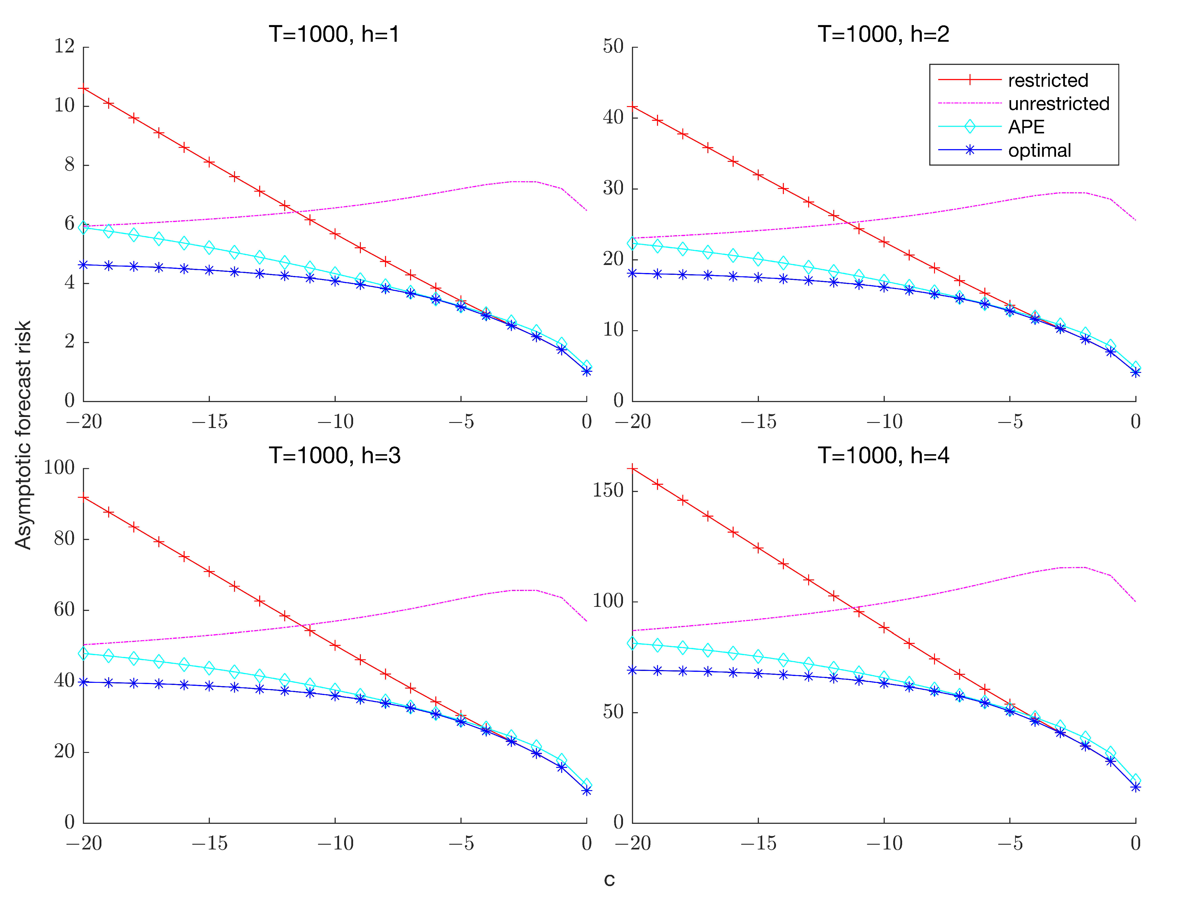
Remark 1.
In a similar vein, Hansen (2010a) developed feasible combination weights by evaluating the Mallows criterion at the two limits of c ,   given that the criterion depends on c   and is therefore infeasible in practice. Thus, while his analysis demonstrated that the infeasible Mallows criterion is an asymptotically unbiased estimate of the AMSE for any c ,   the feasible version of the criterion remains valid only in the two limit cases. When estimation is performed using FGLS instead of OLS, Kejriwal and Yu (2021) showed that the infeasible Mallows criterion also depends on the parameter a   in (1) which governs the short-run dynamics. Evaluating the criterion at the two limits, however, eliminates the dependence on both nuisance parameters.
Figure 2 plots the AFR of the optimal (infeasible) and APE-based combination forecasts for p = 1   and k = 0 .5 For comparison, the unrestricted and restricted forecasts are also presented. As expected, the forecast risk of the restricted estimator increases with c   , while the risk function of the unrestricted estimator is relatively flat as a function of c. Regardless of the forecast horizon, the feasible combination forecast maintains a risk profile close to that of the optimal forecast. In particular, the risk of the APE-weighted forecast is uniformly lower than that of the unrestricted estimator across values of c   , as well as lower than that of the restricted estimator unless c   is very close to zero. These results suggest that the loss in forecast accuracy due to the unknown degree of persistence is relatively small when constructing the combination weights based on the APE criterion. In Section 7 and Section 8, we conduct extensive comparisons of the APE-based combination forecasts with both the Mallows and cross-validation based combination forecasts.

6. Lag Order Uncertainty

This section extends the preceding analysis to the case where the lag order k   is unknown. In order to accommodate lag order uncertainty, the set of models on which the combination forecast is based needs to be expanded to include models with different lag orders. Such a forecast can potentially trade off the misspecification bias inherent from the omission of relevant lags against the problem of overfitting induced by the inclusion of unnecessary lags. Kejriwal and Yu (2021) showed that the essence of this trade-off can be captured analytically by adopting a local asymptotic framework in which the coefficients of the short-run dynamics lie in a O ( T 1 / 2 ) -neighborhood of zero in addition to the O ( T 1 )   parameterization for the persistence parameter as specified in ( 1 ) .   Specifically, we make the following assumption as in Kejriwal and Yu (2021):
Assumption 3.
We assume that α i = δ i T 1 / 2 ,   i = 1 , , k ,   where δ = ( δ 1 , , δ k )   is fixed and independent of T.
Assumption 3 ensures that the squared misspecification bias from omitting relevant lags is of the same order as the sampling variance introduced by estimating additional lags. Modeling { α i }   as fixed would make the bias due to misspecification diverge with the sample size and thus leave no scope for exploiting the trade-off between inclusion and exclusion of lags when constructing the combination forecasts.
We include sub-models with l { 0 , 1 , , K } ,   K k , with the corresponding restricted and unrestricted forecasts given by μ ˜ t ( l )   and μ ^ t ( l ) , respectively. Let I ( l < k ) = 1   if   l < k ,   and zero otherwise. Define ξ h ( δ , l , k ) = M h ( k ) ( 0 l , δ l + 1 , , δ k ) ,   where   0 l   is an ( l × 1 )   vector of zeros. Further, let r h ( δ , l , k ) = ξ h ( δ , l , k ) ξ h ( δ , l , k ) .   The following result derives the AFR of the forecasts in the presence of lag order uncertainty:
Theorem 3.
Under Assumptions 1–3 and sup t   E ( e t θ h ) < ,   where θ h = max { 8 ,   2 ( h + 2 ) } + ψ   for some ψ > 0 ,
(a) lim T T σ 2 E ( μ ^ T + h ( l ) μ T + h ) 2 = h 2 E ( T 1 c 2 ) + g h ( l ) + r h ( δ , l , k ) .
(b) lim T T σ 2 E ( μ ˜ T + h ( l ) μ T + h ) 2 = h 2 E ( T 0 c 2 ) + g h ( l ) + r h ( δ , l , k ) .
Theorem 3 shows that large sample forecast accuracy now depends on an additional misspecification component [ r h ( δ , l , k ) ] emanating from the omission of relevant lags. The larger the magnitudes of the coefficients corresponding to the omitted lags, the larger the contribution of this component to the forecast risk. Moreover, under Assumption 3, g h ( l ) = t r ( M h ( l ) M h ( l ) )   varies with h   for h < l   but is constant for all h l . Similarly, r h ( δ , l , k )   varies with h   for h < k   but is constant thereafter. Thus, the forecast horizon only makes a limited contribution to the two short-run components of the asymptotic forecast risk. Another notable feature of Theorem 3 is that, in contrast to the case where the lag order is assumed known (Theorem 1), the contribution of the trend component is now proportional to the square of the forecast horizon. This difference is due to the fact that the coefficients b j 1   for all j   since α i 0   for i = 1 , , k   by virtue of Assumption 3.
We consider two types of combination forecasts. The first is a “partial averaging” forecast that only addresses lag order uncertainty by averaging over the K + 1   unrestricted forecasts:
μ ^ t + h ( W ^ ) = l = 0 K w ^ l μ ^ t ( l )
The weights W ^ = ( w ^ 0 , w ^ 1 , , w ^ K )   are obtained by minimizing the APE criterion
A P E P ( W ) = i = m h T h l = 0 K w l ( y i + h μ ^ i + h ( l ) ) 2
where w l 0   ( l = 0 , , K ) ,   l = 0 K w l = 1 . We refer to (6) as the APE-based partial averaging (APA) forecast.
The second forecast is a “general averaging” forecast that accounts for both persistence and lag order uncertainty and thus combines the forecasts from all 2 ( K + 1 )   sub-models:
μ ˘ t + h ( W ˘ ) = l = 0 K w ˘ 1 l μ ^ t ( l ) + w ˘ 0 l μ ˜ t ( l )
The weights W ˘ = ( w ˘ 01 , w ˘ 02 , , w ˘ 0 K , w ˘ 11 , w ˘ 12 , , w ˘ 1 K )   are obtained by minimizing a generalized APE criterion of the form
A P E G ( W ) = i = m h T h l = 0 K w 1 l ( y i + h μ ^ i + h ( l ) ) + w 0 l ( y i + h μ ˜ i + h ( l ) ) 2
where w 1 l 0 , w 0 l 0   ( l = 0 , , K ) ,   l = 0 K ( w 0 l + w 1 l ) = 1 . We refer to ( 8 )   as the APE-based general averaging (AGA) forecast. Comparing the APA and AGA forecasts will serve to isolate the effects of the two sources of uncertainty on forecast accuracy.
The following result establishes the limiting behavior of the APE criterion in the presence of lag-order uncertainty:
Theorem 4.
Let A P E 0 ( l ) = i = m h T h y i + h μ ˜ i + h ( l ) 2 ,   A P E 1 ( l ) = i = m h T h y i + h μ ^ i + h ( l ) 2 . Under Assumptions 1–3 and sup t E ( e t r ) < ,   for some r > 2 ,
(a) For c = O ( T ) , lim T   ( σ 2 log T ) 1 A P E 1 ( l ) σ 2 r h ( δ , l , k ) i = m h T h η i , h 2 = h 2 lim c E ( T 1 c 2 ) + g h ( l ) .
(b) lim c 0   lim T   ( σ 2 log T ) 1 A P E 0 ( l ) σ 2 r h ( δ , l , k ) i = m h T h η i , h 2 = h 2 lim c 0 E ( T 0 c 2 ) + g h ( l ) .
Theorem 4 shows that while APE captures the components of AFR that are attributable to persistence uncertainty and estimation of the short-run dynamics, it does not account for lag-order uncertainty in the limit. As shown in the proof of Theorem 4, this is because the former two components grow at a logarithmic rate while the bias component due to lag order misspecification is bounded [i.e., O ( 1 ) ]. Nonetheless, given that the logarithmic function is slowly varying, it can be expected that in small samples, the APE is still effective at capturing the bias that occurs due to misspecification of the number of lags. Indeed, as shown subsequently in the simulations, the APE criterion offers considerable improvements over its competitors, even under lag-order misspecification.

7. Monte Carlo Simulations

This section reports the results of a set of Monte Carlo experiments designed to (1) evaluate the finite sample performance of the proposed approach relative to extant approaches; (2) quantify the importance of accounting for each source of uncertainty in terms of its effect on finite sample forecast risk. Section 7.1 lays out the experimental design. Section 7.2 details the different forecasting procedures included in the analysis. Section 7.3 and Section 7.4 present the results. Results are obtained for p { 0 , 1 } .   For brevity, we report the results only for p = 1 . The results for p = 0   are qualitatively similar, although the improvements offered by the proposed approach are more pronounced for p = 1   than p = 0 . The full set of results is available upon request.

7.1. Experimental Design

We adopt a design similar to that in Hansen (2010a) and Kejriwal and Yu (2021) to facilitate direct comparisons. The data generating process (DGP) is based on (1) and specified as follows: (a) the innovations e t i . i . d . N ( 0 , 1 ) ;   (b) the trend parameters are set at β 0 = β 1 = 0 ;   (c) the true lag order k { 0 , 6 , 12 }   with α j = ( θ ) j for j = 1 , , k and θ = 0.6 . The maximum number of first-differenced lags included is set at K = 12 .   The sample size is set at T { 100 , 200 } . The local-to-unity parameter c varies from 20 to 0, implying α ranging from 0.8 to 1 for T = 100 and α ranging from 0.9 to 1 for T = 200 . At each c value, the finite-sample forecast risk T E ( μ ^ T + h μ T + h ) 2 is computed for all estimators considered, where h { 1 , 3 , 6 , 12 } . All experiments are based on 10,000 Monte Carlo replications.
We report two sets of results. The first assumes k is known, thereby allowing us to demonstrate the effect of persistence uncertainty on forecast accuracy while abstracting from lag order uncertainty. The second allows k   to be unknown and facilitates the comparison between forecasts that address both forms of uncertainty with those that only account for lag order uncertainty.

7.2. Forecasting Methods

The benchmark forecast in both the known and unknown lag cases is calculated from a standard autoregressive model of order K + 1   estimated by OLS:
y t = β 0 * + β 1 * t + α y t 1 + j = 1 K α j Δ y t j + ϵ t
When the number of lags is assumed to be known (Section 7.3), we compare a set of six forecasting methods: (1) Mallows selection (Mal-Sel); (2) Cross-validation selection (CVh-Sel); (3) APE selection (APE-Sel); (4) Mallows averaging (Mal-Ave); (5) Cross-validation averaging (CVh-Ave); (6) APE averaging (APE-Ave). With an unknown number of lags, the following six methods are compared6: (1) Mallows partial averaging (MPA); (2) Cross-validation partial averaging (CPA); (3) APE partial averaging (APA); (4) Mallows general averaging (MGA); (5) Cross-validation general averaging (CGA); (6) APE general averaging (AGA). For brevity, a detailed description of these methods is not presented here but is included in Appendix B.
Both the APE selection and combination forecasts require a choice of m h . To our knowledge, no data-dependent methods for choosing m h   are available in the existing literature. We therefore examined the viability of alternative choices via simulations. Specifically, for each persistence level (value of c), we computed the minimum forecast risk over all values of m h   in the range [ 15 , 70 ]   with a step-size of 5 (assuming a known number of lags k). While no single value was found to be uniformly dominant across persistence levels/horizons, m h = 20   turned out to be a reasonable choice overall.
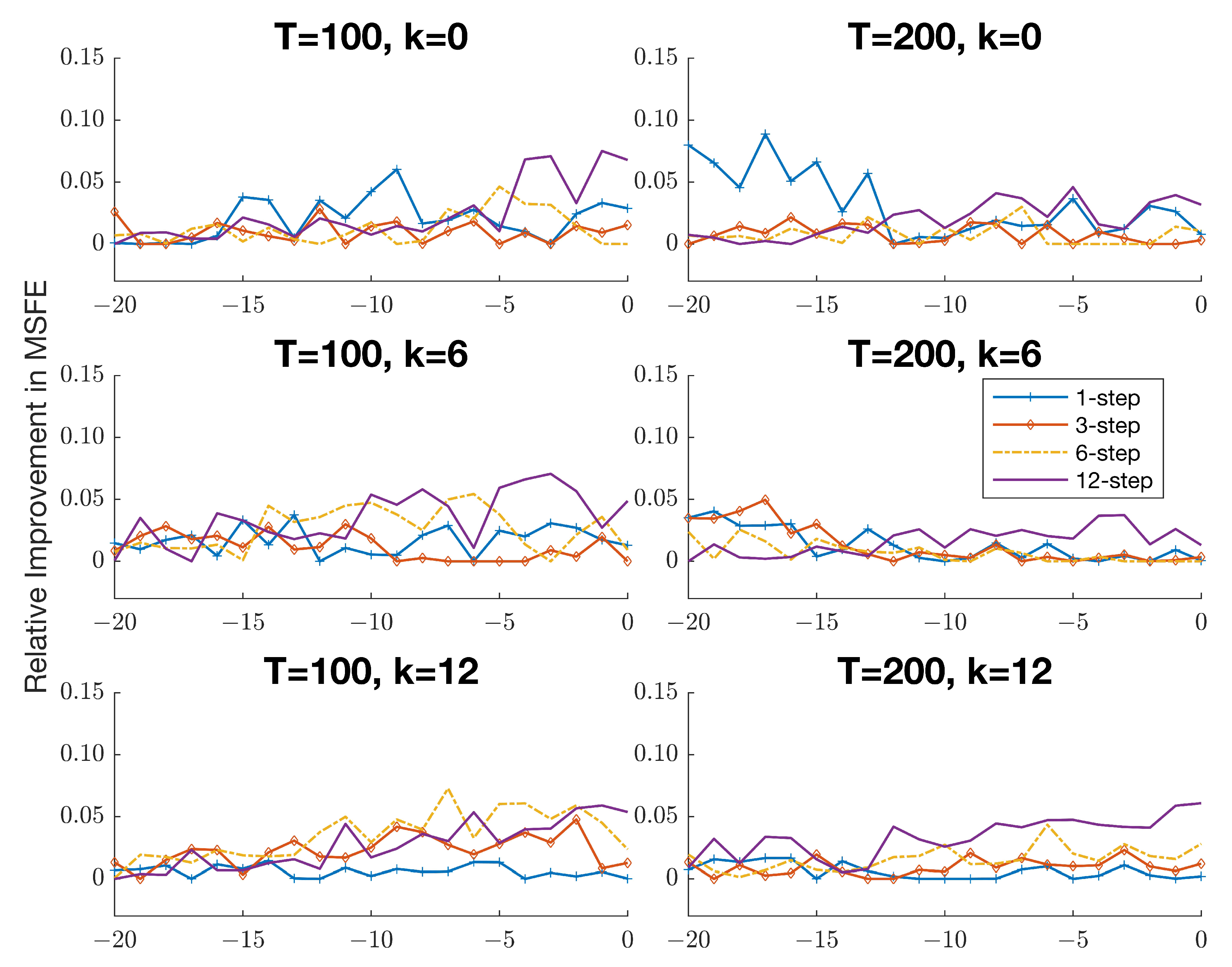
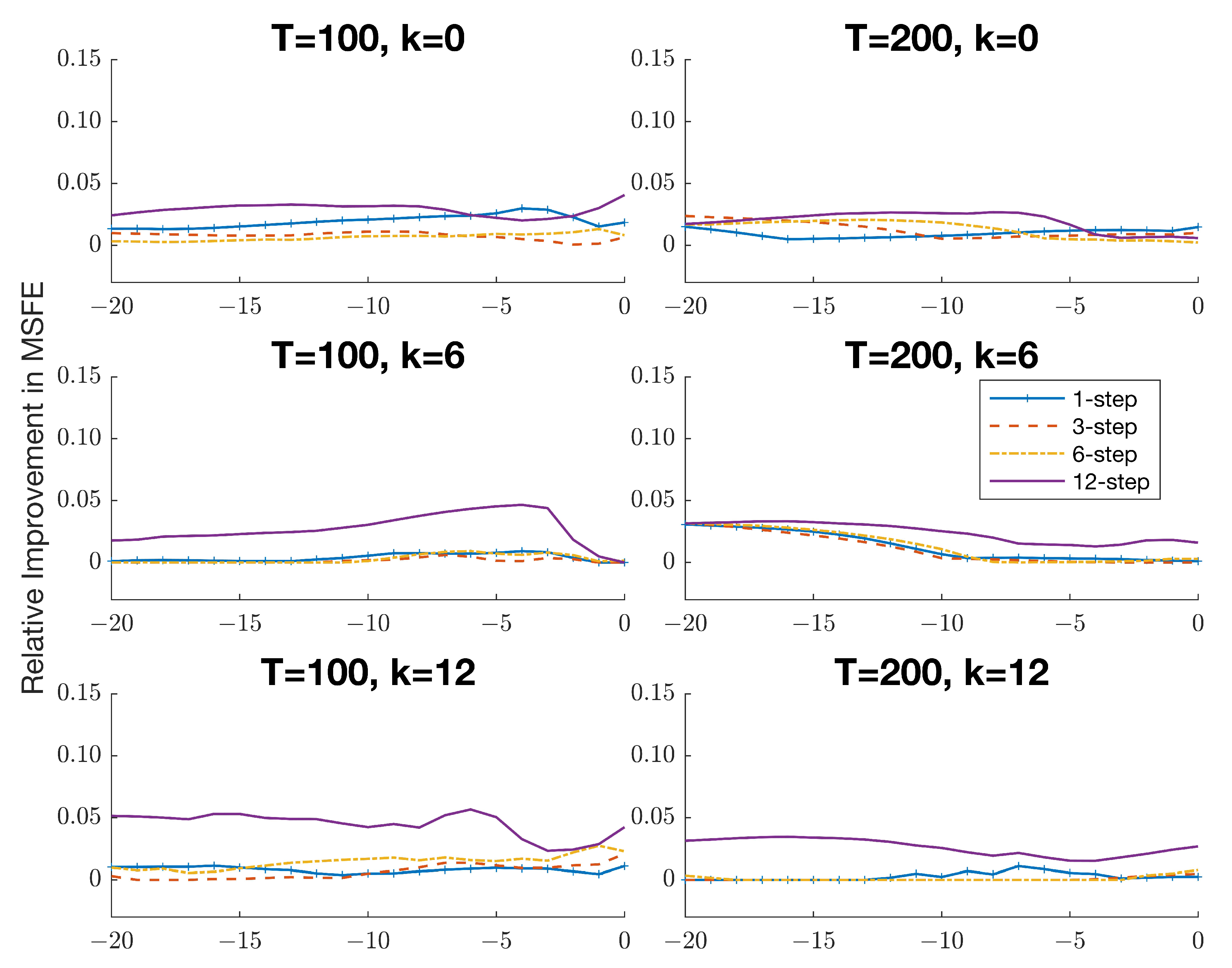
7 To justify this choice, Figure A1 in Appendix C plots the difference between the optimal forecast risk and the risk of the APE selection forecasts for m h = 20   expressed as a percentage of the forecast risk for m h = 20 . The corresponding results for the APE combination forecasts are presented in Figure A2. It is evident that using m h = 20   entails only a marginal increase in forecast risk (at most 5%) for the combination forecasts over the optimal forecast risk across different persistence levels and horizons. In contrast, the optimal choice of m h for the selection forecasts is somewhat more unstable and appears to depend more heavily on the forecast horizon and the level of persistence. This robustness in behavior provides additional motivation for employing a combination approach to forecasting in practice.

7.3. Forecast Risk with Known Lag Order
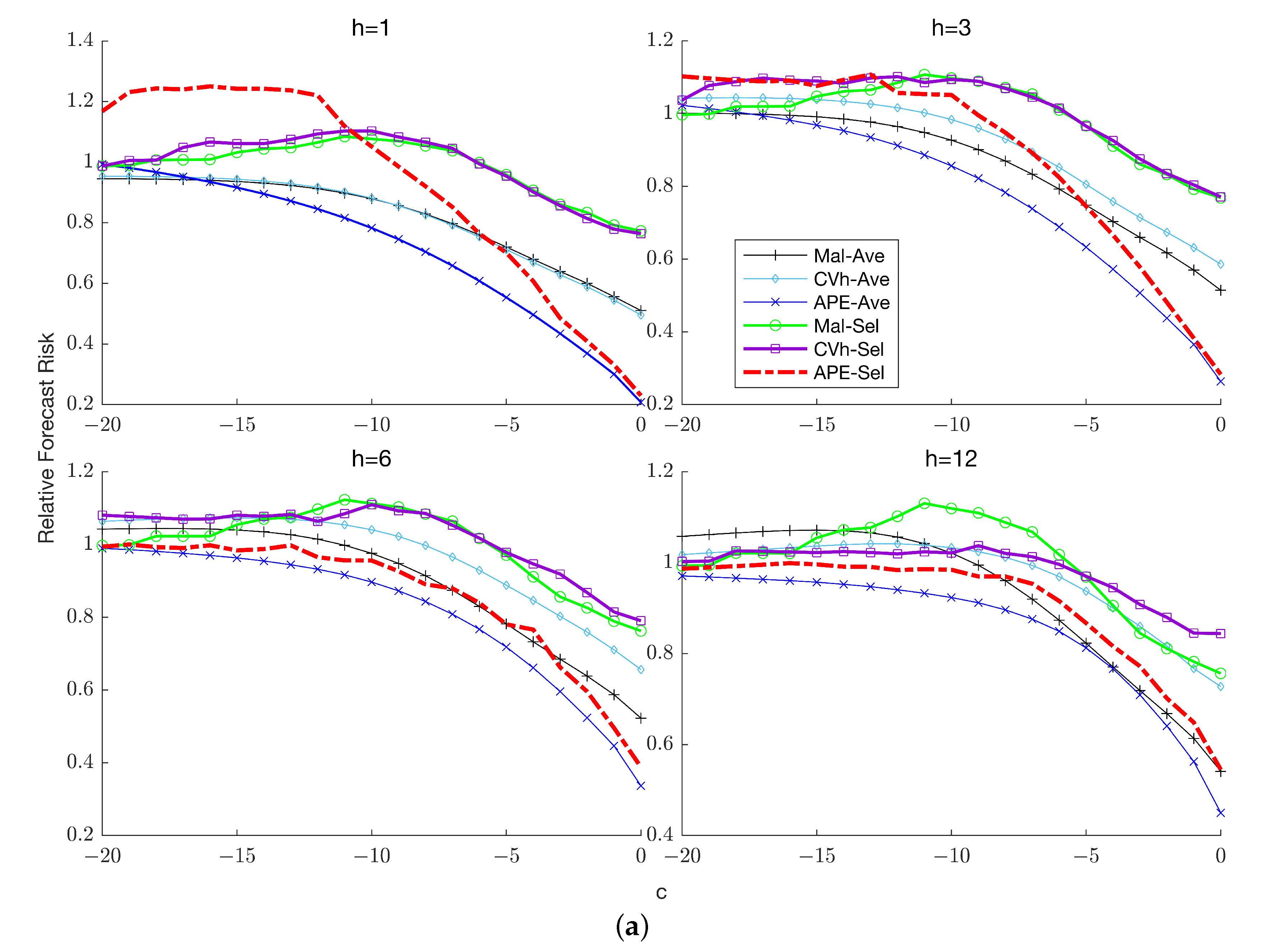
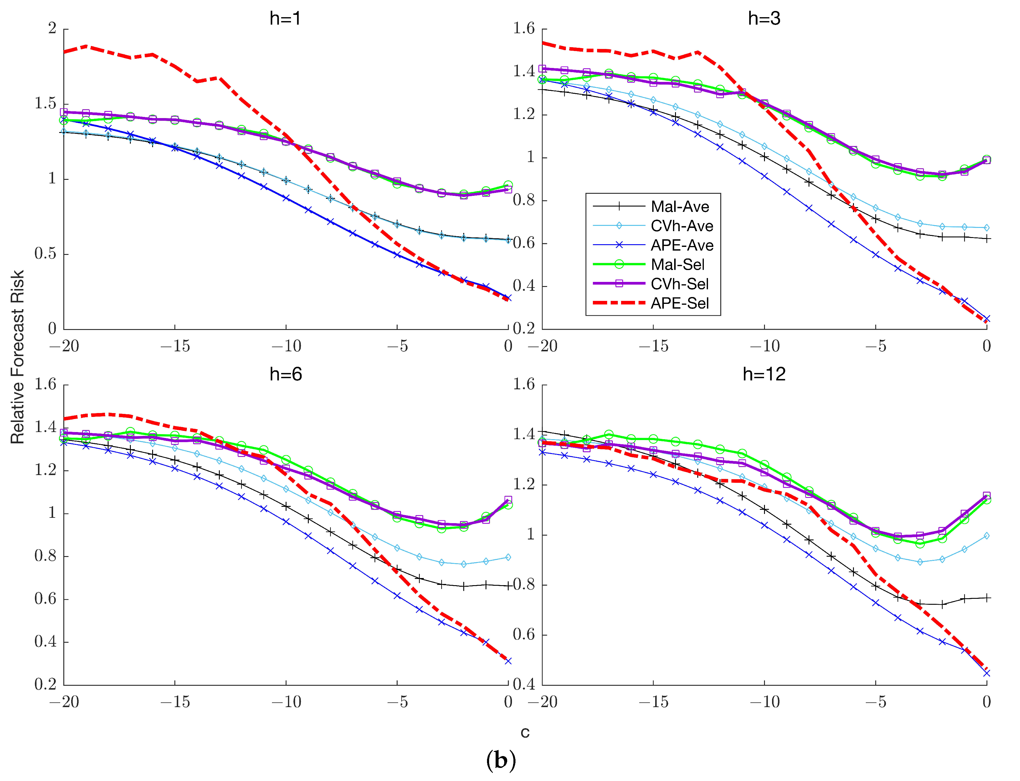
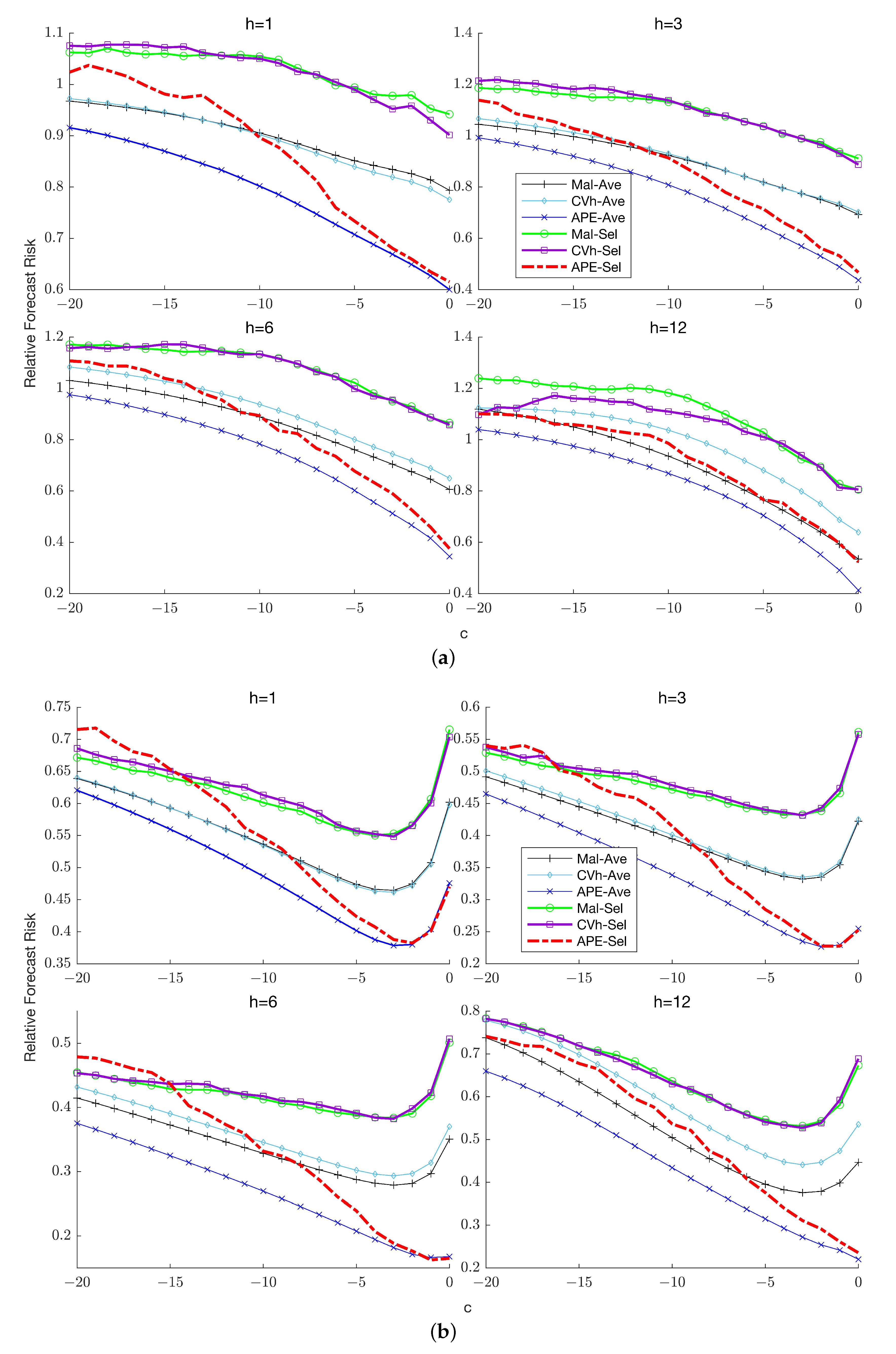
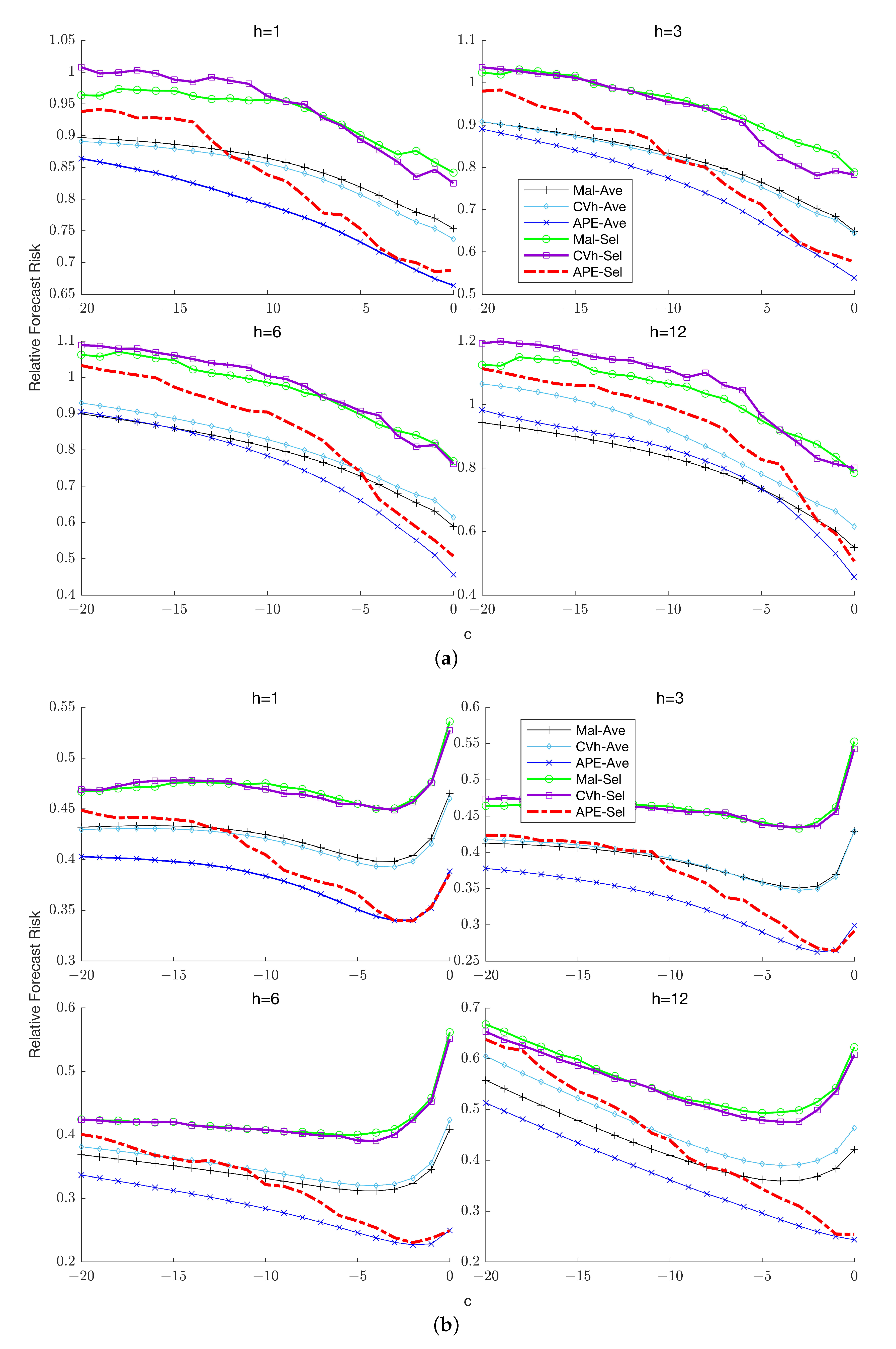
Figure 3a,b, Figure 4a,b and Figure 5a,b plot the risk of the six methods relative to the benchmark. First, we consider the case k = 0 . Several features of the results are noteworthy.
First, the selection forecasts typically exhibit higher risk than the corresponding combination forecasts across sample sizes and horizons. Second, when T = 100 ,   the APE combination forecast is clearly the dominant method, performing discernibly better than forecasts based on either of the two competing weighting schemes. When T = 200 ,   its dominance continues except when | c |   is sufficiently large (the exact magnitude being horizon-dependent), in which case the benchmark delivers the most accurate forecasts and averaging over the restricted model becomes less attractive. Third, the relative performance of the Mallows and cross-validation weighting schemes depends on the horizon: at h = 1 ,   the two schemes yield virtually indistinguishable forecasts; when h { 3 , 6 } ,   Mallows weighting yields uniformly lower risk over the parameter space; at h = 12 ,   Mallows weighting is preferred when persistence is high ( c   close to zero) while cross-validation weighting dominates for lower levels of persistence.
In the presence of higher order serial correlation ( k > 0 ), the superior performance of the APE combination forecast becomes even more evident: it now dominates all competing forecasts regardless of horizon and sample size. In particular, APE weighting outperforms the benchmark at all persistence levels, even at T = 200 ,   unlike the k = 0   case. The intuition for this difference in relative performance between the cases with and without higher-order serial correlation is that in the former case, averaging is comparatively more beneficial, since imposing the unit root restriction can potentially reduce the estimation uncertainty associated with the coefficients of the lagged differences. This reduction in sampling uncertainty in turn engenders a reduction in the overall risk of the combination forecast relative to the unrestricted benchmark forecast. Another notable difference from the k = 0   case is that while Mallows and cross-validation weighting are comparable for h { 1 , 3 } ,   the former now dominates for h { 6 , 12 }   uniformly over the parameter space.

7.4. Forecast Risk with Unknown Lag Order
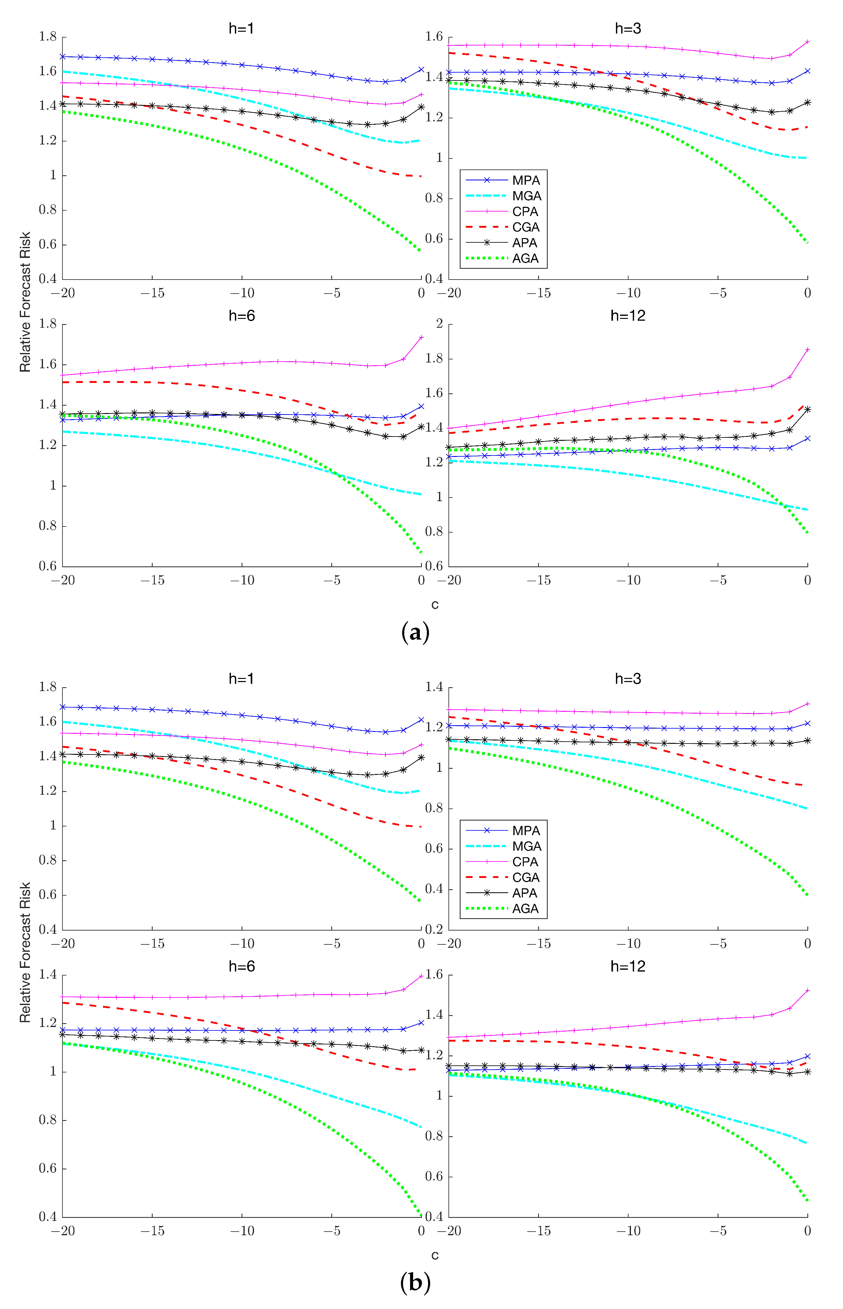
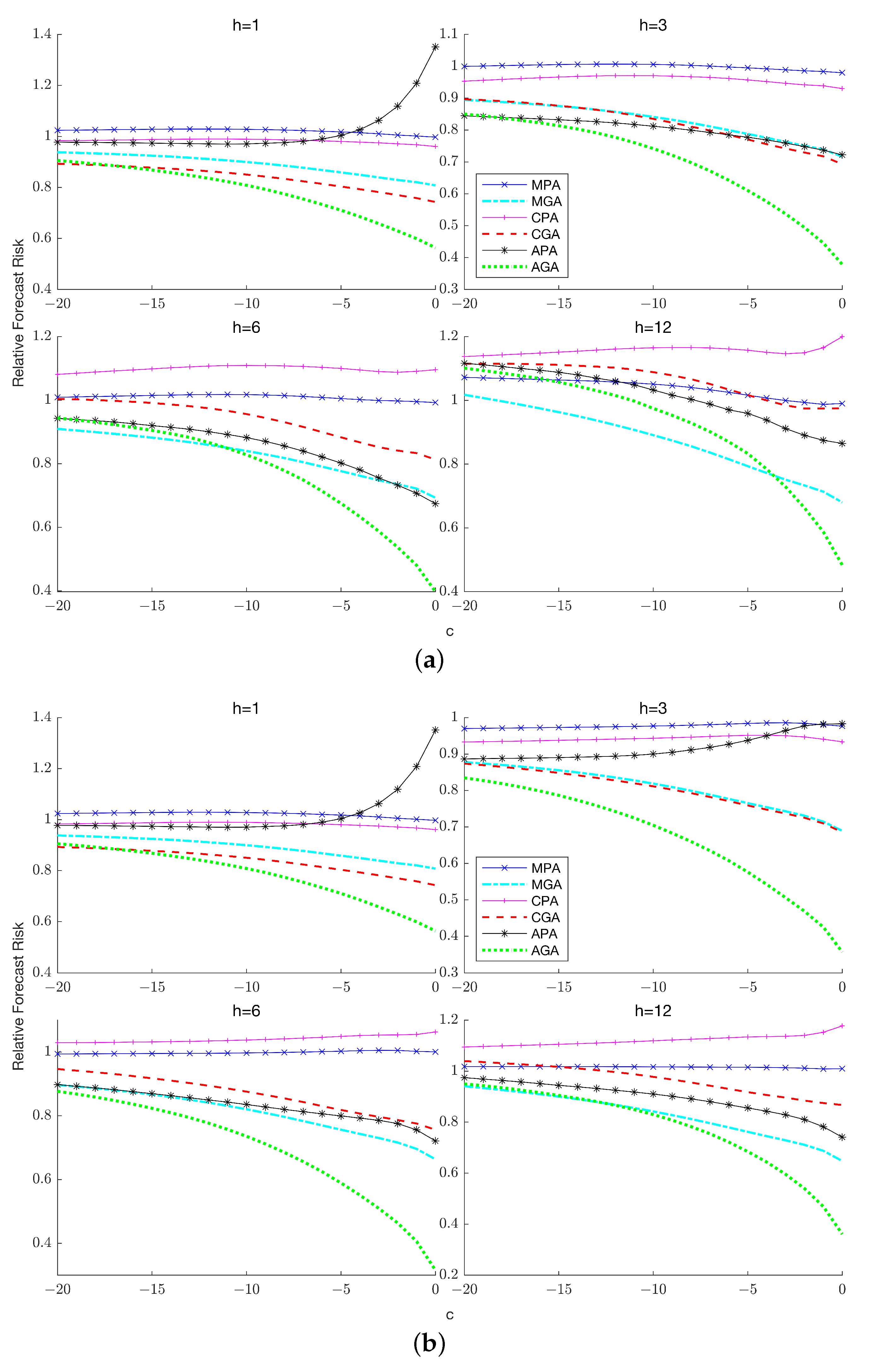
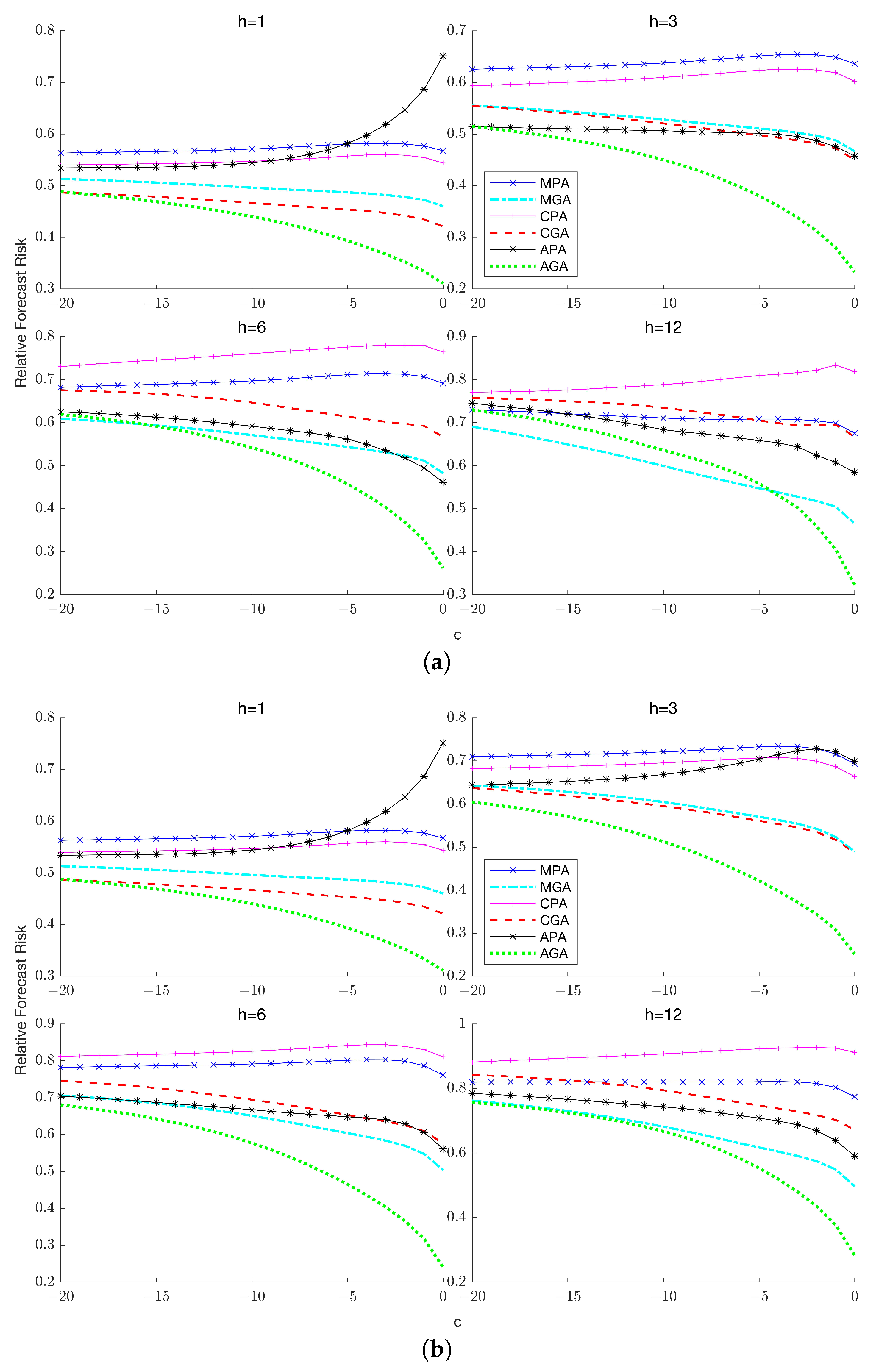
Figure 6a,b, Figure 7a,b and Figure 8a,b plot the relative risk of the six combination forecasts which comprise the three partial forecasts that only account for lag-order uncertainty and the three general forecasts that account for both lag-order and stochastic trend uncertainty. A clear implication of these results is that general averaging methods typically exhibit considerably lower forecast risk than partial averaging methods unless the process has relatively low persistence, in which case averaging over the unit root model increases the forecast risk incurred by the general averaging methods. The improvements offered by general averaging hold across both horizons and the number of lags ( k )   in the true DGP and become more prominent as the sample size increases.
Among the three weighting schemes, APE-based weights are the preferred choice except when h { 6 , 12 }   and T = 100   , where Mallows weighting turns out to be the dominant approach if persistence is relatively low. A potential explanation for this result is that with long horizons and a small sample size, the APE criterion is based on a relatively smaller number of prediction errors, which increases the sampling variability associated with the resulting weights, thereby increasing the risk of the combination forecast. As in the known lag-order case, the choice between Mallows and cross-validation weighting is horizon-dependent: when h = 1 ,   cross-validation weighting is preferred while when h > 1 ,   Mallows weighting is preferred, with the magnitude of reduction in forecast risk increasing as h   increases.
In summary, the results from the simulation experiments make a strong case for employing APE weights when constructing the combination forecasts and clearly highlight the benefits of targeting forecast risk rather than in-sample mean squared error. The comparison of general and partial combination forecasts also underscore the importance of concomitantly controlling for both stochastic trend uncertainty and lag-order uncertainty in generating accurate forecasts.

8. Empirical Application

This section conducts a pseudo out-of-sample forecast comparison of the different multistep forecast combination methods using a set of US macroeconomic time series. Our objectives are to empirically assess (1) the efficacy of different averaging/selection methods relative to a standard autoregressive benchmark; (2) the importance of averaging over both the persistence level and the lag order; and (3) the relative performance of alternative weight choices for constructing the combination forecasts.
Our analysis employs the FRED-MD data set compiled by McCracken and Ng (2016), which contains 123 monthly macroeconomic variables over the period January 1960–December 20188. McCracken and Ng (2016) suggested a set of seven transformation codes designed to render each series stationary: (1) no transformation; (2) Δ y t ;   (3) Δ 2 y t ; (4) log ( y t ) ; (5) Δ log ( y t ) ; (6) Δ 2 log ( y t ) ; (7) Δ ( y t / y t 1 1 ) . To ensure that the series fit our framework, which allows for highly persistent time series with/without deterministic trends, we adopt the following transformation codes as modified by Kejriwal and Yu (2021): (1’) no transformation; (2’) y t ; (3’) Δ y t , (4’) log ( y t ) ; (5’)   log ( y t ) ; (6’)   Δ log ( y t ) ; (7’)   y t / y t 1 1 . For series that correspond to codes (1’) and (4’), we construct the forecasts from a model with no deterministic trend ( p = 0 ), while for the remaining codes, we use forecasts from a model that include a linear deterministic trend ( p = 1 ). We also report results for eight core series as in Stock and Watson (2002), comprising four real and four nominal variables. As in the simulation experiments, four alternative forecast horizons are considered: h { 1 , 3 , 6 , 12 } . We use a rolling window scheme with an initial estimation period of January 1960–December 1969 so that the forecast evaluation period is January 1970–December 2018 (588 observations). The size of the estimation window changes depending on the forecast horizon h. For example, when h = 1 , the initial training sample contains 120 observations from January 1960–December 1969 while for h = 3 , it contains only 118 observations from January 1960–October 1969. This ensures that the forecast origin is January 1970 for all forecast horizons considered. We compare ten different methods in terms of the mean squared forecast error (MSFE) computed as the average of the squared forecast errors: (1) MPA: Mallows partial averaging over the number of lags only in the unrestricted model; (2) MGA: Mallows general averaging over both the unit root restriction and the number of lags; (3) CPA: leave-h-out cross-validation (CV-h) averaging over the number of lags only in the unrestricted model; (4) CGA: leave-h-out cross-validation averaging over both the unit root restriction and the number of lags; (5) APA: accumulated prediction error averaging over the number of lags only in the unrestricted model; (6) AGA: accumulated prediction error averaging over both the unit root restriction and the number of lags; (7) MS: Mallows selection from all models (unrestricted and restricted) that vary with the number of lags; (8) CVhS: leave-h-out cross-validation selection from all models (unrestricted and restricted) that vary with the number of lags; (9) APES: accumulated prediction error selection from all models (unrestricted and restricted) that vary with the number of lags; (10) AR: unrestricted autoregressive model (benchmark). The maximum number of allowable first differenced lags in each method is set at K = 12 . The benchmark forecast is computed from unrestricted OLS estimation of an autoregressive model of the form (10) that uses 12 first-differenced lags of the dependent variable and includes/excludes a deterministic trend depending on the transformation code the series corresponds to, as discussed above.
Table 1a ( h = 1 , 3 ) and Table 1b ( h = 6 , 12 ) report the percentages of wins and losses based on the MSFE for the 123 series. Specifically, they show the percentage of 123 series for which a method listed in a row outperforms a method listed in a column, and all other methods (last column). A summary of the results in Table 1(a and b) is given below:
  • The averaging methods uniformly dominate their selection counterparts at all forecast horizons. For instance, Mallows/cross-validation averaging outperform the corresponding selection procedures in more than 90% of the series at each horizon. The performance of AGA relative to APES is relatively more dependent on the horizon, with improvements observed in 77% (65%) of the series for h = 1   ( h = 12 ), respectively.
  • Given a particular weighting scheme, averaging over both the unit root restriction and number of lags (general averaging) outperforms averaging over only the number of lags (partial averaging) at all horizons. For instance, when h = 1 ,   MGA (CGA, AGA) dominate MPA (CPA, APA) in 95% (81%, 79%) of the series, respectively, based on pairwise comparisons. A similar pattern is observed for multi-step forecasts.
  • Across all horizons, AGA emerges as the leading procedure due to its ability to deliver forecasts with the lowest MSFE among all methods for the maximum number of series (last column of Table 1(a and b)). This approach also dominates each of the competing approaches in terms of pairwise comparisons. The APES approach ranks second among all methods so that forecasting based on the accumulated prediction errors criterion (either AGA or APES) outperforms the other approaches for more than 50% of the series over each horizon (the specific percentages are 68.3% for h = 1 , 3 ; 57.7% for h = 6 ;   55.3% for h = 12 ).
Next, we examine the performance of the forecasting methods for different types of series based on their groupwise classification by McCracken and Ng (2016) in an attempt to uncover the extent to which the best methods vary by the type of series analyzed. In particular, McCracken and Ng (2016) classified the series into eight distinct groups: (1) output and income; (2) labor market; (3) housing; (4) consumption, orders and inventories; (5) money and credits; (6) interest and exchange rates; (7) prices; (8) stock market. For each of these groups, Table 2 reports the method(s) with the lowest MSFE for the most series compared to all other competing methods. We also report the number of horizons in which (a) averaging outperforms selection and vice-versa; (b) averaging over both the unit root restriction and number of lags (general averaging—GA) methods is superior to averaging over only the number of lags (partial averaging—PA) and vice-versa; (c) each of the three weighting schemes dominates the other two. The results are consistent with those in Table 1(a and b) and clearly demonstrate (1) the dominance of averaging over selection (with the exception of Group 3) ; (2) the benefits of accounting for both stochastic trend uncertainty and lag order uncertainty (GA) relative to only the latter (PA) for five out of the eight groups; (3) the superiority of APE weighting over the two competing weighting schemes (the exception is Group 5, where cross-validation weighting is the dominant approach).
Finally, we present a comparison of the different methods with respect to their ability to forecast the eight core series analyzed in Stock and Watson (2002). Table 3 reports the MSFE of the eight methods relative to the benchmark model (10) for four real variables (industrial production, real personal income less transfers, real manufacturing and trade sales, number of employees on nonagricultural payrolls) while Table 4 reports the corresponding results for four nominal variables (the consumer price index, the personal consumption expenditure implicit price deflator, the consumer price index less food and energy, and the producer price index for finished goods). To assess whether the difference between the proposed methods and the benchmark model is statistically significant, we use a two-tailed Diebold–Mariano test statistic (Diebold and Mariano 1995). A number less than one indicates better forecast performance than the benchmark and vice versa. The method with smallest relative MSFE for a given series is highlighted in bold.
Consider first the results for real variables (Table 3). The performance of the best method is statistically significant (at the 10% level) relative to the benchmark in twelve out of the sixteen cases. Consistent with the results in Table 1(a and b) and Table 2, general averaging typically dominates partial averaging, the exceptions being nonagricultural employment for h 6 ,   industrial production at h = 12 ,   and real manufacturing and trade sales for h = 6 , 12 ,   where APES is the dominant procedure. The AGA approach turns out to have the highest relative forecast accuracy in 50% of all cases, with the improvements offered over rival approaches being particularly notable at h = 12 . While cross-validation weighting does not yield the best forecasting procedure in any of the cases, Mallows weighting is the preferred approach in only two cases, although the improvements are statistically insignificant. Turning to the nominal variables (Table 4), the best method significantly outperforms the benchmark in ten cases. Again, general averaging is usually preferred to partial averaging, the exception being the case h = 12 , where APA outperforms all other methods for three of the four variables. As with the real variables, the AGA forecast is the most accurate in 50% of all cases, though the improvements are now comparable across horizons. Finally, cross-validation weighting partly redeems itself by providing the best forecast in four cases, while Mallows weighting is the preferred method in only one case.
It is useful to briefly discuss the recent, related literature to place our empirical findings in perspective. Cheng and Hansen (2015) conducted a comparison of several shrinkage-type forecasting approaches using 143 quarterly US macroeconomic time series (transformed to stationarity) from 1960 to 2008. Their methods included factor-augmented forecast combination based on Mallows/cross-validation/equal weights, Bayesian model averaging, empirical Bayes, pretesting and bagging. They found that while the methods were comparable at the one-quarter horizon, cross-validation weighting clearly emerged as the preferred approach at the four-quarter horizon. Tu and Yi (2017) found that, when forecasting US inflation one-quarter ahead, Mallows-based combination forecasts that combine forecasts from unrestricted and restricted (imposing no error correction) vector autoregressions under the assumption of cointegration dominated both unrestricted and restricted forecasts. Using the same data set as ours, Kejriwal and Yu (2021) compared partial and general combination forecasts using Mallows weights with forecasts based on pretesting and Mallows selection. Consistent with our results, they found that a general combination strategy that averages over both the unit root restriction and different lag orders delivered the best forecasts overall.
In summary, our empirical results were found to be consistent with the simulation results in that (1) addressing both persistence uncertainty and lag-order uncertainty are crucial for generating accurate forecasts; (2) a weighting scheme that directly targets forecast risk instead of in-sample mean squared error yields an efficacious forecast combination approach at all horizons.

9. Conclusions

This paper has developed new multistep forecast combination methods for a time series driven by stochastic and/or deterministic trends. In contrast to existing methods based on Mallows/cross-validation weighting, our proposed combination forecasts were based on constructing weights obtained from an accumulated prediction errors criterion that directly targets the asymptotic forecast risk instead of the in-sample AMSE. Our analysis found strong evidence in favor of a version of the proposed approach that simultaneously addresses stochastic trend and lag order uncertainty. A practical implication of our results is that the degree of persistence in a time series can play an important role in the choice of combination weights. Our preferred approach can potentially serve as a useful univariate benchmark when evaluating the effectiveness of methods designed to exploit information in large data sets.
We conclude with a discussion of four possible directions for future research. First, the APE-based combination forecasts can potentially be used in conjunction with FGLS estimation of the deterministic component, given that the latter has been shown to yield improved forecasts over OLS estimation (Kejriwal and Yu 2021). Second, it may be useful to explore the possibility of allowing for a nonlinear deterministic component through, say, the inclusion of polynomial trends or a few low-frequency trigonometric components (Gallant 1981). To the extent that the specific nonlinear modeling structure captures the observed nonlinearities, such an approach may contribute to a further improvement in forecasting performance. Third, it would be useful to develop prediction intervals around our combination forecasts in order to quantify the associated sampling uncertainty. Fourth, and perhaps most challenging, while our numerical and empirical analyses clearly document the desirability of the proposed approach based on APE weighting relative to Mallows/CV weighting, an analytical comparison may shed further light on the relative merits of the different methods. To our knowledge, such results are primarily available in the context of the standard stationary framework with Mallows/cross-validation weighting (e.g., Hansen 2007; Zhang et al. 2013; Liao and Tsay 2020). Extending these results to the present nonstationary framework would be a potentially fruitful endeavor.

Author Contributions

Conceptualization, M.K., L.N. and X.Y.; methodology, M.K., L.N. and X.Y.; Software, L.N. and X.Y.; validation, M.K., L.N. and X.Y.; formal analysis, M.K., L.N. and X.Y.; investigation, M.K., L.N. and X.Y.; resources, M.K., L.N. and X.Y.; data curation, L.N. and X.Y.; writing—original draft preparation, M.K., L.N. and X.Y.; writing—review and editing, M.K., L.N. and X.Y.; visualization, L.N. and X.Y.; supervision, M.K.; project administration, M.K. All authors have read and agreed to the published version of the manuscript.

Funding

Yu is supported by Shanghai Sailing Program No. 23YF1402000 and National Natural Science Foundation of China (72303040, 72192845).

Data Availability Statement

The data set is publicly available for download at https://research.stlouisfed.org/econ/mccracken/fred-databases/ (accessed on 1 February 2023) . Simulation data are available upon request.

Acknowledgments

The authors wish to thank the three anonymous referees for their constructive feedback which helped improve the paper. They also gratefully acknowledge many useful discussions from participants in the Purdue University seminar and the Midwest Econometrics conference.

Conflicts of Interest

The authors declare no conflict of interest.

Appendix A. Proofs

Let W ( . ) denote a standard Brownian motion on [ 0 , 1 ] and define the Ornstein-Uhlenbeck process: d W c ( r ) = c W c ( r ) + d W ( r ) . For p { 0 , 1 } ,   let X c ( r ) = ( r p , W c ( r ) )   and define the detrended processes
W c * ( r , p ) = W c ( r ) W c ( r ) 0 1 W c ( s ) d s if if p = 0 p = 1 X c * ( r , p ) = X c ( r ) X c ( r ) 0 1 X c ( s ) d s if if p = 0 p = 1
and the functionals
T 0 c = c W c * ( 1 , p ) + I ( p = 1 ) W ( 1 ) T 1 c = X c * ( 1 , p ) 0 1 X c * ( r , p ) X c * ( r , p ) 1 0 1 X c * ( r , p ) d W ( r ) + I ( p = 1 ) W ( 1 ) .
Let β = ( β 0 , β 1 ) , z t = ( 1 , t ) . Without loss of generality, we assume that β 0 = β 1 = 0   in the true data generating process. For a matrix A ,   A 2 = sup v = 1 v A A v   with v   denoting the Euclidean norm for vector v. Unless otherwise defined, for any variable x , we use x *   to denote its demeaned version. For a random quantity δ , we write δ = δ 0 + o p ( δ 0 ) as δ = δ 0 + s . o . , where s . o . represents a term of smaller order in probability. For brevity, all proofs are provided only for the case p = 1 . The proofs for p = 0   are simpler andfollow analogous arguments.
We start by noting that if u t   is generated by (1), it has the A R ( k + 1 )   representation u t = i = 1 k + 1 a i u t i + e t ,   where a 1 = α + α 1 ,     a i = α i α i 1   ( i = 2 , , k ) ,   a k + 1 = α k . The companion VAR(1) form of the model is expressed as
Y t = B ( k ) Y t 1 + ν t
where
Y t ( k + 3 ) × 1 = ( 1 , t + 1 , y t , , y t k ) , ν t ( k + 3 ) × 1 = ( 0 , 0 , e t , 0 , , 0 ) B ( k ) ( k + 3 ) × ( k + 3 ) = B 1 B 2 0 ( k + 1 ) × 2 F ( k ) , B 1 ( 2 × 2 ) = 1 1 0 1 , B 2 2 × ( k + 1 ) = 0 0 0 0 0 0 F ( k ) ( k + 1 ) × ( k + 1 ) = a ( k )   | I k 0 k ,   F 0 ( k ) = I k + 1 ,     a ( k ) = ( a 1 , , a k + 1 )
With “hat” and “tilde” denoting the unrestricted and restricted OLS estimates, respectively, the unrestricted and restricted forecasts can then be expressed as (see, e.g., Ing 2003):
μ ^ T + h = y T ( k + 1 ) B ^ h 1 ( k ) γ ^ ( k )
μ ˜ T + h = y T ( k + 1 ) B ˜ h 1 ( k ) γ ˜ ( k )
where y T ( k + 1 ) = ( 1 ,   T + 1 ,   y T , , y T k ) ,   γ ^ ( k ) = ( β ^ 0 * , β ^ 1 * , a ^ 1 , , a ^ k + 1 )   and
B ^ ( k ) ( k + 3 ) × ( k + 3 ) = B 1 B ^ 2 0 ( k + 1 ) × 2 F ^ ( k ) , B 1 ( 2 × 2 ) = 1 1 0 1 ,     B ^ 2 2 × ( k + 1 ) = β ^ 0 * 0 0 β ^ 1 * 0 0 F ^ ( k ) ( k + 1 ) × ( k + 1 ) = a ^ ( k )   | I k 0 k ,   F ^ 0 = I k + 1 ,     a ^ ( k ) = ( a ^ 1 , , a ^ k + 1 ) B ˜ ( k ) ( k + 3 ) × ( k + 3 ) = B 1 B ˜ 2 0 ( k + 1 ) × 2 F ˜ ( k ) ,     B ˜ 2 2 × ( k + 1 ) = β ˜ 0 * 0 0 0 0 0
The matrix F ˜ ( k )   is constructed in the same way as F ^ ( k )   with a ^ ( k )   replaced by a ˜ ( k ) , where a ˜ ( k ) = ( a ˜ 1 , , a ˜ k + 1 ) = ( 1 + α ˜ 1 , α ˜ 2 α ˜ 1 , , α ˜ k α ˜ k 1 , α ˜ k ) with γ ˜ ( k ) = ( β ˜ 0 * , 0 , a ˜ 1 , , a ˜ k + 1 ) . Next, we state a set of lemmas that will be useful in developing the proofs of the main results. Lemmas A.1–A.4, A.7–A.9 below parallel Lemmas A.1–A.4, B.1–B.3 in Ing et al. (2009) who assumed an exact unit root ( c = 0 ) .   Since the sample moments have the same order whether c = 0   or c < 0 , the proofs of the following lemmas also follow directly those in Ing et al. (2009) and are hence omitted.
Lemma A1.
Suppose { y t } satisfies (1) and Assumptions 1 and 2. Then for any q > 0 ,
E | | R ^ T 1 ( k ) | | q = O ( 1 )
where
R ^ T ( k ) = T 1 D T ( k ) j = k + 1 T 1 y j ( k + 1 ) y j ( k + 1 ) D T ( k )
with
D T ( k ) ( k + 3 ) × ( k + 3 ) = d i a g ( 1 , T 1 , D ¯ T ( k ) ) , D ¯ T ( k ) ( k + 1 ) × ( k + 1 ) = 1 T α 1 T α k T 1 1 0 0 0 0 0 0 1 1
Lemma A2.
Suppose { y t } satisfies (1) and Assumptions 1 and 2 and for some q 1 2 , sup t E | e t | 2 q 1 < . Then for any 0 < q < q 1 ,
E | | R ^ T 1 ( k ) R ^ T * 1 ( k ) | | q = O ( T q / 2 )
where
R ^ T * ( k ) ( k + 3 ) × ( k + 3 ) = d i a g ( R ^ c * ( k ) 3 × 3 , Γ ^ T ( k ) ) k × k R ^ c * ( k ) = T 1 ( T 1 k ) T 1 j = k + 1 T 1 X t T 1 j = k + 1 T 1 X t T 2 j = k + 1 T 1 X t X t X t = [ T 1 ( t + 1 ) ,   T 1 / 2 N t ] ,   N j = A ( L ) y j Γ ^ T ( k ) = T 1 j = k + 1 T 1 s j ( k ) s j ( k ) ,   s j ( k ) = ( Δ y j , , Δ y j k + 1 )
Lemma A3.
Suppose { y t } satisfies (1) and Assumptions (1) and (2) with sup t E | e t | q <   for some q 2 . Then,
E | | T 1 / 2 D T ( k ) j = k + 1 T 1 y j ( k + 1 ) e j + 1 | | q = O ( 1 )
Lemma A4.
Suppose { y t } satisfies (1) and Assumptions 1 and 2 with sup t E | e t | r <   for some r > 4 . Then,
lim T E ( F T , k ) = 0
where
F T , k = s T ( k ) M h ( k ) Γ ^ T 1 ( k ) j = k + 1 T 1 s j ( k ) e j + 1 X T j = k + 1 T 1 X j X j 1 j = k + 1 T 1 X j e j + 1
Lemma A5.
Let X T × ( p + 1 ) = [ X 1 , X 2 ] T × 1     T × p , X 1 = ( 1 , , 1 ) , and assume X X is invertible. Define M 1 = I T × T X 1 ( X 1 X 1 ) 1 X 1 , X 2 * = M 1 X 2 . For any T × 1 vector e and any p × 1 vector x 2 , we have x ( X X ) 1 X e = x 1 ( X 1 X 1 ) 1 X 1 e + x 2 * ( X 2 * X 2 * ) 1 X 2 * e , where x = ( x 1 , x 2 ) , x 1 = 1 , x 2 * = x 2 ( X 1 X 1 ) 1 X 2 X 1 .
Lemma A6.
Under Assumptions 1 and 2, T β ˜ 0 * σ d W c ( 1 ) .
Lemma A7.
Under Assumptions 1 and 2 and sup t E | e t | q <   for some q > 2 ,
(i) For some κ 1 > 0 , | | Γ ^ ( k ) Γ ( k ) | | = o ( T κ 1 )   a . s . ;
(ii) For some κ 2 > 0 , | | R ^ T R ^ T * | | = o ( T κ 2 )   a . s . ;
(iii) | | R ^ T 1 | | = O ( log log T )   a . s . .
Lemma A8.
Under Assumptions 1 and 2 and sup t E | e t | q <   for some q > 2 , i = m h T h F i , k = o ( T )   a . s . , where
F i , k = s i ( k ) M h ( k ) Γ ^ i 1 ( k ) j = k + 1 i 1 s j ( k ) e j + 1 X i j = k + 1 i 1 X j X j 1 j = k + 1 i 1 X j e j + 1
Lemma A9.
Let { x T } be a sequence of real numbers.
(i) If x T 0 , T 1 j = 1 T x j = O ( 1 ) , and for some ξ > 1 , lim inf T   ν T / T ξ > 0 , then, j = 1 T x j / ν j = O ( 1 ) ;
(ii) If T 1 j = 1 T x j = o ( 1 ) , then, j = 1 T x j / j = o ( log T ) .
Proof of Lemma A5. 
Note, by block matrix inversion,
( X X ) 1 = X 1 X 1 X 1 X 2 X 2 X 1 X 2 X 2 1 = ( X 1 X 1 ) 1 + ( X 1 X 1 ) 1 X 1 X 2 ( X 2 M 1 X 2 ) 1 X 2 X 1 ( X 1 X 1 ) 1 ( X 1 X 1 ) 1 X 1 X 2 ( X 2 M 1 X 2 ) 1 ( X 2 M 1 X 2 ) 1 X 2 X 1 ( X 1 X 1 ) 1 ( X 2 M 1 X 2 ) 1
then
( X X ) 1 X e = ( X 1 X 1 ) 1 X 1 [ I X 2 ( X 2 M 1 X 2 ) 1 X 2 M 1 ] e ( X 2 M 1 X 2 ) 1 X 2 M 1 e
Recall x = ( x 1 , x 2 ) = ( x 1 , x 2 * ) + ( 0 , X 1 X 2 ( X 1 X 1 ) 1 ) , we have,
x ( X X ) 1 X e = [ ( x 1 , x 2 * ) ] ( X X ) 1 X e Term 1 + [ ( 0 , X 1 X 2 ( X 1 X 1 ) 1 ) ] ( X X ) 1 X e Term 2 = x 1 ( X 1 X 1 ) 1 X 1 [ I X 2 ( X 2 M 1 X 2 ) 1 X 2 M 1 ] e + x 2 * ( X 2 M 1 X 2 ) 1 X 2 M 1 e Term 1 + X 1 X 2 ( X 1 X 1 ) 1 ( X 2 M 1 X 2 ) 1 X 2 M 1 e Term 2 = x 1 ( X 1 X 1 ) 1 X 1 e + x 2 * ( X 2 M 1 X 2 ) 1 X 2 M 1 e x 1 ( X 1 X 1 ) 1 X 1 X 2 ( X 2 M 1 X 2 ) 1 X 2 M 1 e + X 1 X 2 ( X 1 X 1 ) 1 ( X 2 M 1 X 2 ) 1 X 2 M 1 e = 0 ,   since x 1   =   1 , ( X 1 X 1 ) 1 =   1 / T , which is a constant = x 1 ( X 1 X 1 ) 1 X 1 e + x 2 * ( X 2 * X 2 * ) 1 X 2 * e
Proof of Lemma A6. 
The true DGP can be expressed as
Δ y t = β 0 * + j = 1 k α j Δ y t j + e t *
where β 0 * = 0 and e t * = a c T u t 1 + e t . Let Z ˙ t = ( Z ˙ 1 , Z ˙ 2 , t ) , Z ˙ 1 = 1 , Z ˙ 2 , t = ( Δ y t 1 , , Δ y t k ) , ι 1 = ( 1 , 0 , , 0 ) , ι [ 2 : k + 1 ] = ( 0 , 1 , , 1 ) . Now
T β ˜ 0 * σ = T σ ι 1 ( t = k + 1 T Z ˙ t Z ˙ t ) 1 t = k + 1 T Z ˙ t ( a c T u t 1 + e t ) = T σ ( t = k + 1 T Z ˙ 1 2 ) 1 t = k + 1 T Z ˙ 1 ( a c T u t 1 + e t ) + o p ( 1 ) = c a σ T 3 / 2 t = k + 1 T u t 1 + 1 σ T t = k + 1 T e t + o p ( 1 ) d c 0 1 W c + W ( 1 ) = W c ( 1 )
Proof of Theorem 1. 
(a) Defining γ ( k ) = ( β 0 * , β 1 * , a 1 , , a k + 1 ) ,   L ^ h ( k ) = j = 0 h 1 b j B ^ h 1 j ( k ) and L h = j = 0 h 1 b j B h 1 j ( k ) , we can write
T σ 2 E ( μ ^ T + h μ T + h ) 2 = T σ 2 E y T ( k + 1 ) L ^ h ( k ) ( γ ^ ( k ) γ ( k ) ) 2 = T σ 2 [ E y T ( k + 1 ) L h ( k ) ( γ ^ ( k ) γ ( k ) ) 2 + E y T ( k + 1 ) L ^ h ( k ) L h ( k ) ( γ ^ ( k ) γ ( k ) ) 2 + o ( 1 ) ] = 1 σ 2 E y T ( k + 1 ) L h ( k ) D T ( k ) ( R ^ T * 1 ( k ) ) D T ( k ) T j = k + 1 T 1 y j ( k + 1 ) e j + 1 2 + 1 σ 2 E y T ( k + 1 ) L h ( k ) D T ( k ) ( R ^ T 1 ( k ) R ^ T * 1 ( k ) ) D T ( k ) T j = k + 1 T 1 y j ( k + 1 ) e j + 1 2 + T σ 2 E y T ( k + 1 ) L ^ h ( k ) L h ( k ) ( γ ^ ( k ) γ ( k ) ) 2 + o ( 1 ) = ( I ) + ( I I ) + ( I I I )
The ( I I ) and ( I I I ) terms in (A5) are each o ( 1 ) by Lemmas A1–A3 and Holder’s inequality [see, e.g., the proof of Theorem 2.2 in Ing et al. 2009].
The term ( I ) can be written as:
1 σ 2 E y T ( k + 1 ) L h ( k ) D T ( k ) R ^ T * 1 ( k ) D T ( k ) T j = k T 1 y j ( k + 1 ) e j + 1 2 = 1 σ 2 E y T ( k + 1 ) D T ( k ) L ¯ h ( k ) R ^ T * 1 ( k ) D T ( k ) T j = k T 1 y j ( k + 1 ) e j + 1 2
where L ¯ h ( k ) = j = 0 h 1 b j d i a g ( G T h 1 j , F ¯ ( k ) h 1 j ) with G T = 1 T 1 0 1 , F ¯ ( k ) = d i a g ( 1 , S M ( k ) ) and S M ( k ) = α ( k 1 ) I k 1 α k 0 k 1   ,   S M 0 ( k ) = I k .
Note that y T ( k + 1 ) D T = 1 , T 1 ( T + 1 ) , T 1 / 2 N T , s T ( k ) . Further, since G T is upper triangular, (A6) converges to
1 σ 2 j = 0 h 1 b j 2 lim T E T 1 / 2 j = k + 1 T 1 e j + 1 + X T * j = k + 1 T 1 X j * X j * 1 j = k + 1 T 1 X j * e j + 1 2 + lim T 1 σ 2 E s T ( k ) M h ( k ) Γ ^ T 1 ( k ) T 1 / 2 j = k + 1 T 1 s j ( k ) e j + 1 2 + 2 σ 2 ( j = 0 h 1 b j ) lim T E ( F T , k ) = B. 1 + B. 2 + B. 3
where B. 1 utilizes Lemma A.5. Since B. 2 = g h ( k ) by Theorem 1 of Ing (2003) and B. 3 = 0 by Lemma A4, (A7) simplifies to:
B. 1 + B. 2 = j = 0 h 1 b j 2 lim T E W ( 1 ) + X c * ( 1 ) 0 1 X c * X c * 1 0 1 X c * d W 2 + g h ( k ) = j = 0 h 1 b j 2 E T 1 c 2 + g h ( k )
The required result then follows from (A5), (A7) and (A8).
(b) Defining L ˜ h ( k ) = j = 0 h 1 b j B ˜ h 1 j ( k ) , with similar arguments as in (a), we can write:
T σ 2 E ( μ ˜ T + h μ T + h ) 2 = T σ 2 E y T ( k + 1 ) L ˜ h ( k ) ( γ ˜ ( k ) γ ( k ) ) 2 = T σ 2 E y T ( k + 1 ) L h ( k ) ( γ ˜ ( k ) γ ( k ) ) 2 + o ( 1 )
Note that
L h ( k ) = j = 0 h 1 b j B h 1 j ( k ) = j = 0 h 1 b j B 1 0 0 F ( k ) h 1 j = j = 0 h 1 b j B 1 h 1 j 0 0 F h 1 j ( k )
Since B 1   is upper triangular with B 1 ( 1 , 1 ) = 1 ,
( A 9 ) = T σ 2 E y T ( k + 1 ) j = 0 h 1 b j β ˜ 0 * 0 j = 0 h 1 b j F h 1 j ( k ) [ a ˜ ( k ) a ( k ) ] 2 + o ( 1 ) = T σ 2 E j = 0 h 1 b j β ˜ 0 * + ( y T , , y T k ) j = 0 h 1 b j F h 1 j ( k ) [ a ˜ ( k ) a ( k ) ] 2 + o ( 1 )
Now, consider the term
T σ ( y T , , y T k ) j = 0 h 1 b j F h 1 j ( k ) [ a ˜ ( k ) a ( k ) ] = T σ ( y T , , y T k ) L h ( F ) ( k ) [ a ˜ ( k ) a ( k ) ] = T σ ( y T , , y T k ) L h ( F ) ( k ) a ^ ( k ) a ( k ) + H k D T ( k ) R ^ T 1 ( k ) D T ( k ) R k ( R k D T ( k ) R ^ T 1 ( k ) D T ( k ) R k ) 1 ( r R k γ ^ ( k ) )
where
L h ( F ) ( k ) = j = 0 h 1 b j F ( k ) h 1 j , H k ( k + 1 ) × ( k + 3 ) = 0 ( k + 1 ) × 2 I ( k + 1 ) , R k 2 × ( k + 3 ) = 0 1 0 0 0 0 1 1 , r 2 × 1 = ( 0 , 1 )
Next, define L ¯ h ( F ) ( k ) = d i a g ( j = 0 h 1 b j , M h ( k ) ) , θ ^ ( k ) ( k + 1 ) × 1 = ( T ( 1 α ^ ) / a , 0 , , 0 ) , we have
( A 11 ) = 1 σ ( y T , , y T k ) T L h ( F ) ( k ) { a ^ ( k ) a ( k ) } + L h ( F ) ( k ) D ¯ T ( k ) θ ^ ( k ) = 1 σ ( y T , , y T k ) T L h ( F ) ( k ) { a ^ ( k ) a ( k ) } + D ¯ T ( k ) L ¯ h ( F ) ( k ) θ ^ ( k ) = 1 σ ( y T , , y T k ) T L h ( F ) ( k ) ( a ^ ( k ) a ( k ) ) + 1 σ ( N T / T , s T ( k ) ) d i a g ( j = 0 h 1 b j , M h ( k ) ) θ ^ ( k ) = 1 σ ( y T , , y T k ) T L h ( F ) ( k ) ( a ^ ( k ) a ( k ) ) + N T σ T j = 0 h 1 b j c T ( α ^ α ) / a = N T σ T j = 0 h 1 b j T ( α ^ α ) / a + 1 σ s T ( k ) M h ( k ) Γ ^ T 1 ( k ) T 1 / 2 j = k T 1 s j ( k ) e j + 1 + N T σ T j = 0 h 1 b j c T ( α ^ α ) / a = c N T σ T j = 0 h 1 b j + 1 σ s T ( k ) M h ( k ) Γ ^ T 1 ( k ) T 1 / 2 j = k T 1 s j ( k ) e j + 1
Then, combining (A10) with (A12) and using Lemma A6, we finally get
lim T T σ 2 E ( μ ˜ T + h μ T + h ) 2 = E j = 0 h 1 b j ( W c ( 1 ) c W c ( 1 ) ) 2 + 1 σ 2 lim T E s T * ( k ) M h ( k ) Γ ^ T 1 ( k ) T 1 / 2 j = k T 1 s j ( k ) e j + 1 2 = j = 0 h 1 b j 2 E T 0 c 2 + g h ( k )
which uses the fact that W c ( 1 ) c W c ( 1 ) = W ( 1 ) c W c * ( 1 ) , thereby proving the result. □
Proof of Theorem 2. 
Henceforth, estimated parameters and quantities with subscript i denotes the estimates using observations from 1 to i. We prove (a) first. It follows from Chow (1965) and Ing (2004) that
A P E 1 i = m h T h η i , h 2 = i = m h T h y i ( k + 1 ) L ^ i , h ( k ) ( γ ^ i ( k ) γ ( k ) ) 2 ( 1 + o ( 1 ) ) + O ( 1 )     a . s .
Using similar algebra as in Theorem 1, we have:
i = m h T h y i ( k + 1 ) L ^ i , h ( k ) ( γ ^ i ( k ) γ ( k ) ) 2 = i = m h T h [ y i ( k + 1 ) L h ( k ) ( γ i ^ ( k ) γ ( k ) ) 2 + y i ( k + 1 ) L ^ i , h ( k ) L h ( k ) ( γ ^ i ( k ) γ ( k ) ) 2 ] + s . o . = i = m h T h 1 i y i ( k + 1 ) L h ( k ) D i ( k ) ( R ^ i * 1 ( k ) ) D i ( k ) i j = k + 1 i 1 y j ( k + 1 ) e j + 1 2 + i = m h T h 1 i y i ( k + 1 ) L h ( k ) D i ( k ) ( R ^ i 1 ( k ) R ^ i * 1 ( k ) ) D i ( k ) i j = k + 1 i 1 y j ( k + 1 ) e j + 1 2 + i = m h T h y i ( k + 1 ) L ^ i , h ( k ) L h ( k ) ( γ ^ i ( k ) γ ( k ) ) 2 + s . o . = ( I V ) + ( V ) + ( V I )
The ( V ) and ( V I ) terms in (A13) are each O ( 1 ) following similar arguments in Ing et al. (2009) which build on Lemmas A7–A9.
Analogous to (A6) and (A7) in the proof of Theorem 1, (IV) can be rewritten as:
( I V ) = j = 0 h 1 b j 2 i = m h T h Z i j = k + 1 i 1 Z j Z j 1 j = k + 1 i 1 Z j e j + 1 2 + i = m h T h s i ( k ) M h ( k ) Γ ^ i 1 ( k ) 1 i j = k + 1 i 1 s j ( k ) e j + 1 2 + 2 ( j = 0 h 1 b j ) i = m h T h 1 i F i , k = C. 1 + C. 2 + C. 3
where Z j = ( 1 , t + 1 , N j ) . In analogy with Theorem 3.1 of Ing (2004),
C . 2 = g h ( k ) σ 2 log T + o p ( log T )
By Lemmas A8 and A9, C . 3 = o p ( log T ) . Now we focus on C . 1 . By Theorem 4 of Wei (1987), we have
C . 1 = j = 0 h 1 b j 2 σ 2 log det ( j = k + 1 T 1 Z j Z j ) + o p ( log T )
Defining the 3 × 3 matrix Υ T = d i a g ( T , T 3 , T 2 / c )   and using Lemma A of Phillips (2014) in conjunction with the fact that c T 2 = O ( T 1 ) , we can calculate
log det ( j = k + 1 T 1 Z j Z j ) = log det ( Υ T 1 / 2 Υ T 1 / 2 j = k + 1 T 1 Z j Z j Υ T 1 / 2 Υ T 1 / 2 ) = log det ( Υ T ) + O p ( 1 ) = log ( T 5 ) + O p ( 1 ) = 5 log ( T ) + O p ( 1 )
which leads to C . 1 = 5 σ 2 j = 0 h 1 b j 2 log ( T ) + o p ( log T ) . Thus,
lim T 1 σ 2 log T ( A P E 1 i = m h T h η i , h 2 ) = 5 j = 0 h 1 b j 2 + g h ( k )
where the right hand side of (A16) is the limit of f 1 ( c , p , k , h ) = f 1 ( c , p , h ) + g h ( k ) as c -.
We next prove (b). Following similar steps as in the proof of (a) and the proof of Theorem 1 for the restricted case, we can derive
A P E 0 i = m h T h η i , h 2 = j = 0 h 1 b j 2 i = m h T h ( β ˜ 0 , i * c N i i ) 2 + i = m h T h s i ( k ) M h ( k ) Γ ^ i 1 ( k ) 1 i j = k + 1 i 1 s j ( k ) e j + 1 2 + o p ( log T ) = D. 1 + D. 2
In view of (A4), taking the limit c 0 , we have
i = m h T h ( β ˜ 0 , i * c N i i ) 2 = i = m h T h [ ι 1 ( t = k + 1 i Z ˙ t Z ˙ t ) 1 t = k + 1 i Z ˙ t e t ] 2 = i = m h T h [ ( t = k + 1 i Z ˙ 1 2 ) 1 t = k + 1 i Z ˙ 1 e t ] 2 + s . o . = log det ( j = k + 1 T 1 Z ˙ 1 2 ) + o p ( log T ) = σ 2 log T + o p ( log T )
Further, using the same argument as in (A14), we have D . 2 = g h ( k ) σ 2 log T + o p ( log T ) . Thus,
lim c 0 lim T 1 σ 2 log T ( A P E 0 i = m h T h η i , h 2 ) = j = 0 h 1 b j 2 + g h ( k )
where the right hand side of (A17) is the limit of f 0 ( c , p , k , h ) = f 0 ( c , p , h ) + g h ( k ) as c 0   since lim c 0 E ( T 0 c 2 ) = E [ W ( 1 ) 2 ] = 1 . □
For the proofs of Theorems 3 and 4, we focus on the misspecified case where l < k . For the case l k ,   the proofs follow directly from the arguments in Theorems 1 and 2 above and those in Ing et al. (2009).
Proof of Theorem 3. 
First, note that under Assumption 3, Lemmas A1–A4 continue to hold with k   replaced by l   ( l < k ) , and e t replaced by ε t = e t + ω t ,   where ω t = j = l + 1 k α j Δ y t j . Define L h * ( l ) = j = 0 h 1 b j B * ( l ) h 1 j ,   where B * ( l )   is defined similarly to B ( l )   except that F ( l )   is replaced by F * ( l ) = a * ( l )     | I l 0 l ,     F * 0 ( l ) = I l + 1 ,   a * ( l ) = ( a 1 , , a l , a l + 1 * )   and a l + 1 * = α l . Also, let γ * ( l ) = ( β 0 * , β 1 * , a 1 , , a l , a l + 1 * )   and α * ( l , k ) = ( 0 l , α l + 1 , , α k ) . Finally, note that under Assumption 3, b j 1   for all j.
(a) We can write
T σ 2 E ( μ ^ T + h ( l ) μ T + h ) 2 = T σ 2 E y T ( l + 1 ) L ^ h ( l ) ( γ ^ ( l ) γ * ( l ) ) + s T ( k ) M h ( k ) α * ( l , k ) 2 = E [ f ^ T , h 2 ( l , k ) ] + E [ r T , h 2 ( l , k ) ] + o ( 1 ) = ( I ) + ( I I ) + o ( 1 )
where
f ^ T , h ( l , k ) = ( T / σ ) y T ( l + 1 ) L ^ h ( l ) ( γ ^ ( l ) γ * ( l ) ) r T , h ( l , k ) = ( T / σ ) s T ( k ) M h ( k ) α * ( l , k )
We now derive the limit of the terms ( I )   and ( I I )   in (A18). First, consider the term ( I )   in (A18). Noting that the effective errors are now { ε t }   instead of { e t } ,   we can write, similar to (A5),
E [ f ^ T , h 2 ( l , k ) ] = 1 σ 2 E y T ( l + 1 ) L h * ( l ) D T ( l ) ( R ^ T * 1 ( l ) ) D T ( l ) T j = l + 1 T 1 y j ( l + 1 ) ε j + 1 2 + 1 σ 2 E y T ( l + 1 ) L h * ( l ) D T ( l ) ( R ^ T 1 ( l ) R ^ T * 1 ( l ) ) D T ( l ) T j = l + 1 T 1 y j ( l + 1 ) ε j + 1 2 + T σ 2 E y T ( l + 1 ) L ^ h ( l ) L h * ( l ) ( γ ^ ( l ) γ * ( l ) ) 2 + o ( 1 ) = ( T 1 ) + ( T 2 ) + ( T 3 ) + o ( 1 )
The terms ( T 2 )   and ( T 3 )   are each o ( 1 )   by the fact that Lemmas A1–A3 hold when { e t }   is replaced by { ε t } . Now consider the following term appearing in term ( T 1 ) :
D T ( l ) T j = l + 1 T 1 y j ( l + 1 ) ε j + 1 = D T ( l ) T j = l + 1 T 1 y j ( l + 1 ) e j + 1 + D T ( l ) T j = l + 1 T 1 y j ( l + 1 ) ω j + 1 = D T ( l ) T j = l + 1 T 1 y j ( l + 1 ) e j + 1 + 1 T i = l + 1 k δ i j = l + 1 T D T ( l ) y j ( l + 1 ) Δ y j i + 1 = D T ( l ) T j = l + 1 T 1 y j ( l + 1 ) e j + 1 + 1 T i = l + 1 k δ i 1 T j = l + 1 T D T ( l ) y j ( l + 1 ) e j i + 1 + o p ( 1 ) = D T ( l ) T j = l + 1 T 1 y j ( l + 1 ) e j + 1 + 1 T i = l + 1 k δ i O p ( 1 ) + o p ( 1 ) = D T ( l ) T j = l + 1 T 1 y j ( l + 1 ) e j + 1 + o p ( 1 )
where the third equality follows from Assumption 3. Then, substituting (A20) in (A19) and following the same arguments used in deriving (A8), we get
lim T E [ f ^ T , h 2 ( l , k ) ] = lim T ( T 1 ) = h 2 E ( T 1 c 2 ) + g h ( l )
Now, consider the term ( I I )   in (A18). Defining ξ h ( δ , l , k ) = M h ( k ) ( 0 l , δ l + 1 , , δ k ) ,   we can write
E [ r T , h 2 ( l , k ) ] = 1 σ 2 T α * ( l , k ) M h ( k ) E { s T ( k ) s T ( k ) } M h ( k ) T α * ( l , k ) = 1 σ 2 T α * ( l , k ) M h ( k ) σ 2 I k M h ( k ) T α * ( l , k ) + o ( 1 ) ξ h ( δ , l , k ) ξ h ( δ , l , k )
where the second equality in (A22) follows from the facts that under Assumption 3, T α * ( l , k ) = ( 0 l , δ l + 1 , , δ k ) and E { s T ( k ) s T ( k ) } σ 2 I k . Finally, substituting (A21) and (A22) in (A18), the result follows.
(b) We can write
T σ 2 E ( μ ˜ T + h ( l ) μ T + h ) 2 = T σ 2 E y T ( l + 1 ) L ˜ h ( l ) ( γ ˜ ( l ) γ * ( l ) ) + s T ( k ) M h ( k ) α * ( l , k ) 2 = E [ f ˜ T , h 2 ( l , k ) ] + E [ r T , h 2 ( l , k ) ] + o ( 1 ) = ( I ) + ( I I ) + o ( 1 )
where f ˜ T , h ( l , k ) = ( T / σ ) y T ( l + 1 ) L ˜ h ( l ) ( γ ˜ ( l ) γ * ( l ) )   and r T , h ( l , k )   is as defined in (A18). The limit of term ( I I )   is derived in (A22). To obtain the limit of ( I ) ,   we follow the same steps as in the proof of Theorem 1(b) with k   replaced by l   and use (A20) to get
E [ f ˜ T , h 2 ( l , k ) ] h 2 E ( T 0 c 2 ) + g h ( l )
The result then follows by substituting (A24) and (A22) in (A23). □
Proof of Theorem 4. 
(a) For each i { m h , T h } , we can write
y i + h μ ^ i + h ( l ) = η i , h y i ( l + 1 ) L ^ i , h ( l ) ( γ ^ i * ( l ) γ * ( l ) ) f ^ i , h ( l , k ) + s i ( k ) M h ( k ) α * ( l , k ) r i , h ( l , k )
We then have
A P E 1 ( l ) = i = m h T h η i , h f ^ i , h ( l , k ) + r i , h ( l , k ) 2 = i = m h T h η i , h 2 + i = m h T h f ^ i , h 2 ( l , k ) [ 1 + o p ( 1 ) ] + i = m h T h r i , h 2 ( l , k ) + 2 i = m h T h η i , h r i , h ( l , k ) 2 i = m h T h f ^ i , h ( l , k ) r i , h ( l , k ) + O p ( 1 )
Note that i = m h T h η i , h r i , h ( l , k ) = T 1 / 2 i = m h T h η i , h s i ( k ) M h ( k ) T 1 / 2 α * ( l , k ) = O p ( 1 ) . O ( 1 ) = O p ( 1 ) . We will now consider i = m h T h f ^ i , h 2 ( l , k ) , i = m h T h r i , h 2 ( l , k ) , and i = m h T h f ^ i , h ( l , k ) r i , h ( l , k ) in turn.
i = m h T h f ^ i , h 2 ( l , k ) = i = m h T h 1 i y i ( l + 1 ) L h ( l ) D i ( l ) R ^ i * 1 ( l ) D i ( l ) i j = l i 1 y j ( l + 1 ) ε j + 1 2 + O p ( 1 )   = i = m h T h 1 i y i ( l + 1 ) L h ( l ) D i ( l ) R ^ i * 1 ( l ) D i ( l ) i j = l i 1 y j ( l + 1 ) e j + 1 2 + O p ( 1 ) = 5 σ 2 h 2 log T + g h ( l ) σ 2 log T + o p ( log T ) .
where the first equality in (A26) follows in analogy with (A13), the second follows in analogy with (A20), and the third follows from the same arguments used to derive (A14) and (A15) as well as the fact that b j 1 .
Next, consider the term
i = m h T h r i , h 2 ( l , k ) = i = m h T h α * ( l , k ) M h ( k ) s i ( k ) s i ( k ) M h ( k ) α * ( l , k ) = ξ h ( δ , l , k ) T 1 i = m h T h s i ( k ) s i ( k ) ξ h ( δ , l , k ) = ξ h ( δ , l , k ) ( σ 2 I k ) ξ h ( δ , l , k ) + o p ( 1 ) σ 2 ξ h ( δ , l , k ) ξ h ( δ , l , k )
where the third equality in (A27) is a consequence of Assumption 3.
Finally, consider the cross-product term
i = m h T h f ^ i , h ( l , k ) r i , h ( l , k ) i = m h T h f ^ i , h 2 ( l , k ) 1 / 2 i = m h T h r i , h 2 ( l , k ) 1 / 2 = O p log T O p ( 1 ) = o p ( log T )
Substituting (A26)–(A28) in (A25), the result follows.
(b) For each i { m h , T h } , we can write
y i + h μ ˜ i + h ( l ) = η i , h y i ( l + 1 ) L ˜ i , h ( l ) ( γ ˜ i * ( l ) γ * ( l ) ) f ˜ i , h ( l , k ) + s i ( k ) M h ( k ) α * ( l , k ) r i , h ( l , k )
We then have
A P E 0 ( l ) = i = m h T h η i , h f ˜ i , h ( l , k ) + r i , h ( l , k ) 2 = i = m h T h η i , h 2 + i = m h T h f ˜ i , h 2 ( l , k ) [ 1 + o p ( 1 ) ] + i = m h T h r i , h 2 ( l , k ) 2 i = m h T h f ˜ i , h ( l , k ) r i , h ( l , k ) + O p ( 1 )
By similar arguments as in (a), we have
i = m h T h f ˜ i , h 2 ( l , k ) = σ 2 h 2 log T + g h ( l ) σ 2 log T + o p ( log T ) i = m h T h f ˜ i , h ( l , k ) r i , h ( l , k ) = o p ( log T )
Substituting (A27) and (A30) in (A29), the result follows. □

Appendix B. Description of Methods

This Appendix provides a detailed description of the forecasting methods compared in the Monte Carlo analysis presented in Section 7 and the empirical analysis presented in Section 8.
Unrestricted Autoregressive Model (Benchmark). The benchmark forecast is calculated from a standard autoregressive model of order K + 1   estimated by OLS:
y t = β 0 * + β 1 * t + α y t 1 + j = 1 K α j Δ y t j + ϵ t ,
Mallows Selection.Hansen (2010a) demonstrated the validity of the Mallows criterion for selecting between the restricted and unrestricted models when h = 1 . When the number of lags k   is known, the criteria for the restricted and unrestricted models are, respectively, given by
M 0 = T σ ˜ 2 + 2 σ ^ 2 ( p + k ) M 1 = T σ ^ 2 + 2 σ ^ 2 ( 2 + p + k )
where σ ˜ 2 = T 1 t = 1 T ( y t μ ˜ t ) 2   and σ 2 = T 1 t = 1 T ( y t μ ^ t ) 2 . The Mallows selection estimator picks the restricted model if M 0 < M 1   and the unrestricted model otherwise. This is equivalent to picking the unrestricted model when F T = T ( σ ˜ 2 σ ^ 2 σ ^ 2 ) 4 . The Mallows selection forecast can then be expressed as μ ^ t + h , M = μ ^ t + h 1 ( F T 4 ) + μ ˜ t + h 1 ( F T < 4 ) . When the number of lags is unknown, the relevant Mallows criteria are obtained as (see Kejriwal and Yu 2021):
M 0 ( l ) = T σ ˜ l 2 + 2 σ ^ K 2 ( p + l ) M 1 ( l ) = T σ ^ l 2 + 2 σ ^ K 2 ( 2 + p + l )
for l = 0 , 1 , , K ,   where σ ^ j 2 = T 1 t = 1 T ( y t μ ^ t ( j ) ) 2 ,   j = l , K   and σ ˜ l 2 = T 1 t = 1 T ( y t μ ˜ t ( l ) ) 2 . Then, defining l ˜ = arg min l S { M 0 ( l ) } ,   l ^ = arg min l S { M 1 ( l ) } ,   where S = { 0 , 1 , , K } ,   the Mallows selection forecast is obtained as
μ ˘ t + h , M = μ ^ t + h ( l ^ ) , μ ˜ t + h ( l ˜ ) , i f i f min l S { M 1 ( l ) } min l S { M 0 ( l ) } min l S { M 1 ( l ) } > min l S { M 0 ( l ) }
Mallows Averaging. As an alternative to Mallows selection, Hansen (2010a) developed the Mallows combination forecast that entails taking a weighted average of the unrestricted and restricted forecasts where the weights are chosen by minimizing a Mallows criterion. When the number of lags is known, the criterion is
M w = t = 1 T ( y t μ ^ t ( w ) ) 2 + 2 σ ^ 2 ( 2 w + p + k )
with μ ^ t ( w ) = w μ ^ t + ( 1 w ) μ ˜ t   and σ ^ 2 = T 1 t = 1 T ( y t μ ^ t ) 2 . The Mallows selected weight w ^ is derived from minimizing (A31) over w [ 0 , 1 ] . The solution is
w ^ = 1 2 / F T 0 i f     F T > 2 o t h e r w i s e
The Mallows averaging estimator is then defined as
μ ^ t + h , M ( w ^ ) = w ^ μ ^ t + h + ( 1 w ^ ) μ ˜ t + h = μ ˜ t + h ( 1 2 F T ) μ ^ t + h + 2 F T μ ˜ t + h i f     F T 2 o t h e r w i s e
When the number of lags is unknown, Hansen (2010a) considered two alternative Mallows combination forecasts. The first is the so-called partial averaging forecast that averages only over unrestricted forecasts that vary according to the number of first-differenced lags included. With a maximum of K   lags, this forecast is given by
μ ^ t + h , M ( W ^ ) = l = 0 K w ^ l μ ^ t + h ( l )
where W ^ = ( w ^ 0 , w ^ 1 , w ^ K )   minimizes the criterion (with μ ^ t ( W ) = l = 0 K w l μ ^ t ( l ) ),
M P ( W ) = t = 1 T ( y t μ ^ t ( W ) ) 2 + 2 σ ^ K 2 l = 0 K [ w l ( 2 + l + p ) ]
subject to the restrictions w j 0   ( j = 0 , 1 , K ) ,   j = 0 K w j = 1 . The second combination forecast is the so-called general averaging forecast that averages over the forecasts from all 2 ( K + 1 )   models that include the ( K + 1 )   restricted models. This forecast is given by
μ ˘ t + h , M ( W ˘ ) = l = 0 K w ˘ 1 l μ ^ t + h ( l ) + w ˘ 0 l μ ˜ t + h ( l )
with W ˘ = ( w ˘ 00 , w ˘ 01 , , w ˘ 0 K , w ˘ 10 , w ˘ 11 , w ˘ 12 , , w ˘ 1 K )   minimizing the criterion (with μ ˘ t ( W ) = l = 0 K w 0 l μ ˜ t ( l ) + w 1 l μ ^ t ( l ) ),
M G ( W ) = t = 1 T ( y t μ ˘ t ( W ) ) 2 + 2 σ ^ K 2 l = 0 K [ w 0 l l + w 1 l ( 2 + l ) ] + p
where the weights are non-negative and sum to one: w 1 l 0 , w 0 l 0 ,   l = 0 K ( w 0 l + w 1 l ) = 1 . In what follows, we will refer to (A33) and (A34) as the MPA (Mallows Partial Averaging) and MGA (Mallows General Averaging) forecasts, respectively.
Leave-h-out Cross Validation Selection.Hansen (2010b) provided theoretical justification for constructing h-step ahead forecasts using leave-h-out cross validation under the assumption that the data are strictly stationary. For model selection with a known number of lags, let C V 0   and C V 1   denote the cross-validation criteria for the restricted and unrestricted models, respectively. These criteria are computed as
C V 0 = t = k + 1 T h ( y t + h μ ˜ t + h ( t ) ) 2
C V 1 = t = k + 1 T h ( y t + h μ ^ t + h ( t ) ) 2
where μ ˜ t + h ( t )   and μ ^ t + h ( t )   are the restricted and unrestricted leave-h-out forecasts, respectively. Specifically, μ ˜ t + h ( t )   is obtained using parameter estimates from the restricted model after leaving out the observations { t + 1 , , t + h } 9:
Δ y j = β 0 * + s = 1 k α k Δ y j s + ϵ j ,       j t + 1 , , t + h
Similarly, μ ^ t + h ( t ) is obtained from estimating the unrestricted model after leaving out the observations { t + 1 , , t + h } :
y j = β 0 * + β 1 * j + α y j 1 + s = 1 k α k Δ y j s + ϵ j ,       j t + 1 , , t + h
Then the cross-validation based forecast is μ ^ t + h , C V = μ ^ t + h 1 ( C V 1 C V 0 ) + μ ˜ t + h 1 ( C V 1 > C V 0 ) .   When the number of lags is unknown, the cross-validation criterion is computed for each of the 2 ( K + 1 )   possible models and the selected forecast, denoted μ ˘ t + h , C V , is the one that corresponds to the model with the minimum value of this criterion.
Leave-h-out Cross Validation Averaging. When the number of lags is known, the cross validation weights ( w ^ , 1 w ^ ) are obtained by minimizing the criterion
C V w = t = k + 1 T h w ( y t + h μ ^ t + h ( t ) ) + ( 1 w ) ( y t + h μ ˜ t + h ( t ) ) 2
and the resulting forecast is μ ^ t + h , C V ( w ^ ) = w ^ μ ^ t + h + ( 1 w ^ ) μ ˜ t + h . When the number of lags is unknown, the partial combination forecast that only combines the unrestricted forecasts with different lags is obtained as
μ ^ t + h , C V ( W ^ ) = l = 0 K w ^ l μ ^ t + h ( l )
where W ^ = ( w ^ 0 , w ^ 1 , w ^ K )   minimizes the criterion
C V P ( W ) = t = k + 1 T h l = 0 K w l ( y t + h μ ^ t + h ( t ) ( l ) ) 2
subject to the restrictions w j 0   ( j = 0 , 1 , , K ) ,   j = 0 K w j = 1 , and μ ^ t + h ( t ) ( l )   is the unrestricted leave-h-out forecast assuming l   first-differenced lags. As with weight selection using the Mallows criterion, we also construct a general combination forecast that combines forecasts from the K + 1   unrestricted models as well as the K + 1   restricted models. This forecast is given by
μ ˘ t + h , C V ( W ˘ ) = l = 0 K w ˘ 1 l μ ^ t + h ( l ) + w ˘ 0 l μ ˜ t + h ( l )
with W ˘ = ( w ˘ 01 , w ˘ 02 , , w ˘ 0 K , w ˘ 11 , w ˘ 12 , , w ˘ 1 K )   minimizing the criterion
C V G ( W ) = t = k + 1 T h l = 0 K w 1 l ( y t + h μ ^ t + h ( t ) ( l ) ) + w 0 l ( y t + h μ ˜ t + h ( t ) ( l ) ) 2
where w 1 l 0 , w 0 l 0 , l = 0 K ( w 0 l + w 1 l ) = 1 ,   μ ^ t + h ( t ) ( l )   is as defined in (A38) and μ ˜ t + h ( t ) ( l )   is the restricted leave-h-out forecast assuming l   first-differenced lags. In what follows, we will refer to (A37) and (A39) as the CPA (Cross-Validation Partial Averaging) and CGA (Cross-Validation General Averaging) forecasts, respectively.
APE Selection. With a known number of lags, this forecast is computed from the model that corresponds to the lower APE between the restricted and unrestricted models:
μ ^ t + h , S = μ ˜ t + h I ( A P E 0 A P E 1 ) + μ ^ t + h I ( A P E 0 > A P E 1 ) A P E 0 = i = m h T h y i + h μ ˜ i + h 2 ,     A P E 1 = i = m h T h y i + h μ ^ i + h 2
In the unknown lags case, the forecast is computed from the model that minimizes the APE criterion among all 2 ( K + 1 )   possible models, comprising the K + 1   restricted and K + 1   unrestricted models.

Appendix C. Additional Simulation Results

This Appendix shows simulation evidence to justify the choice of m h = 20 . Figure A1 and Figure A2 plot the difference between the optimal forecast risk (a grid from 20 to 70 in increments of 5) and the risk of the APE selection and APE averaging forecasts respectively for m h = 20   expressed as a percentage of the forecast risk for m h = 20 .
Figure A1. Forecast risk with optimal m h and m h = 20 , APE selection ( p = 1 ) .
Econometrics 11 00028 g0a1
Figure A2. Forecast risk with optimal m h and m h = 20 , APE averaging ( p = 1 ) .
Econometrics 11 00028 g0a2

Notes

1
Analytically, the importance of the trend component over long horizons can be seen by noting that the trend/drift coefficient is multiplied by the forecast horizon when constructing forecasts so that any specification/estimation error is magnified linearly as the forecast horizon increases (Sampson 1991).
2
The conclusion for the subsequent analysis will not be affected as long as the initial observations are o p ( T 1 / 2 ) .
3
The figure was obtained by simulating the AMSE and AFR assuming i.i.d. normal errors with T = 1000 . 5000 replications were used.
4
To illustrate the lack of uniformity, consider the case p = 1   with k = 0 . Using the same arguments as in the proof of Theorem 2 of Yu et al. (2012), it follows that, for any finite c 0 ,   i = m h T h y i + h μ ^ i + h 2 = E ( T 10 2 ) log T + o p ( log T ) ,   where E ( T 10 2 ) = 6 . The lack of uniformity follows since E ( T 1 c 2 ) E ( T 10 2 )   for any c < 0 .
5
This figure was obtained using the same method as in Figure 1.
6
We do not report the results for the selection forecasts, since their performance relative to the combination forecasts is qualitatively similar to the known lag-order case. The results are nevertheless available upon request.
7
This choice was also adopted by Ing and Yang (2014) in their Monte Carlo analysis of forecasting using autoregressive models with positive-valued errors.
8
The data set is publicly available for download at https://research.stlouisfed.org/econ/mccracken/fred-databases/ (accessed on 1 February 2023).
9
Hansen (2010b) instead left out the 2 h 1 observations { t h + 1 , , t , t + 1 , , t + h 1 } . The difference emanates from the fact that he constructs direct forecasts while our forecasts are constructed iteratively which exploit the autoregressive structure and hence necessitate leaving out only the h   observations { t + 1 , , t + h } .

References

  1. Bates, John M., and Clive W. J. Granger. 1969. The combination of forecasts. Journal of the Operational Research Society 20: 451–68. [Google Scholar] [CrossRef]
  2. Box, George E. P., and Gwilym M. Jenkins. 1970. Time Series Analysis: Forecasting and Control. San Francisco: Holden-Day. [Google Scholar]
  3. Cheng, Xu, and Bruce E. Hansen. 2015. Forecasting with factor-augmented regression: A frequentist model averaging approach. Journal of Econometrics 186: 280–93. [Google Scholar] [CrossRef]
  4. Chow, Yuan Shih. 1965. Local convergence of martingales and the law of large numbers. The Annals of Mathematical Statistics 36: 552–58. [Google Scholar] [CrossRef]
  5. Clements, Michael P., and David F. Hendry. 2001. Forecasting with difference-stationary and trend-stationary models. The Econometrics Journal 4: 1–19. [Google Scholar]
  6. Diebold, Francis X., and Lutz Kilian. 2000. Unit-root tests are useful for selecting forecasting models. Journal of Business & Economic Statistics 18: 265–73. [Google Scholar]
  7. Diebold, Francis X., and Roberto S. Mariano. 1995. Comparing predictive accuracy. Journal of Business and Economic Statistics 13: 253–63. [Google Scholar]
  8. Elliott, Graham. 2006. Unit Root Pre-Testing and Forecasting. Technical Report, Working Paper. San Diego: UCSD. [Google Scholar]
  9. Gallant, A. Ronald. 1981. On the bias in flexible functional forms and an essentially unbiased form: The fourier flexible form. Journal of Econometrics 15: 211–45. [Google Scholar] [CrossRef]
  10. Gonzalo, Jesus, and Jean-Yves Pitarakis. 1998. On the exact moments of asymptotic distributions in an unstable ar(1) with dependent errors. International Economic Review 39: 71–88. [Google Scholar] [CrossRef]
  11. Granger, Clive W. J. 1966. The typical spectral shape of an economic variable. Econometrica 34: 150–61. [Google Scholar] [CrossRef]
  12. Hamilton, James Douglas. 1994. Time Series Analysis. Princeton: Princeton University Press. [Google Scholar]
  13. Hansen, Bruce E. 2007. Least squares model averaging. Econometrica 75: 1175–89. [Google Scholar] [CrossRef]
  14. Hansen, Bruce E. 2008. Least-squares forecast averaging. Journal of Econometrics 146: 342–50. [Google Scholar] [CrossRef]
  15. Hansen, Bruce E. 2010a. Averaging estimators for autoregressions with a near unit root. Journal of Econometrics 158: 142–55. [Google Scholar] [CrossRef]
  16. Hansen, Bruce E. 2010b. Multi-step forecast model selection. Paper presented at the 20th Annual Meetings of the Midwest Econometrics Group, St. Louis, MO, USA, October 1–2. [Google Scholar]
  17. Ing, Ching-Kang. 2001. A note on mean-squared prediction errors of the least squares predictors in random walk models. Journal of Time Series Analysis 22: 711–24. [Google Scholar] [CrossRef]
  18. Ing, Ching-Kang. 2003. Multistep prediction in autoregressive processes. Econometric Theory 19: 254–79. [Google Scholar] [CrossRef]
  19. Ing, Ching-Kang. 2004. Selecting optimal multistep predictors for autoregressive processes of unknown order. The Annals of Statistics 32: 693–722. [Google Scholar] [CrossRef]
  20. Ing, Ching-Kang, Jin-Lung Lin, and Shu-Hui Yu. 2009. Toward optimal multistep forecasts in non-stationary autoregressions. Bernoulli 15: 402–37. [Google Scholar] [CrossRef]
  21. Ing, Ching-Kang, Chor-yiu Sin, and Shu-Hui Yu. 2012. Model selection for integrated autoregressive processes of infinite order. Journal of Multivariate Analysis 106: 57–71. [Google Scholar] [CrossRef]
  22. Ing, Ching-Kang, and Chiao-Yi Yang. 2014. Predictor selection for positive autoregressive processes. Journal of the American Statistical Association 109: 243–53. [Google Scholar] [CrossRef]
  23. Kejriwal, Mohitosh, and Xuewen Yu. 2021. Generalized forecast averaging in autoregressions with a near unit root. The Econometrics Journal 24: 83–102. [Google Scholar] [CrossRef]
  24. Kim, Hyun Hak, and Norman R. Swanson. 2018. Mining big data using parsimonious factor, machine learning, variable selection and shrinkage methods. International Journal of Forecasting 34: 339–54. [Google Scholar] [CrossRef]
  25. Liao, Jen-Che, and Wen-Jen Tsay. 2020. Optimal multistep var forecast averaging. Econometric Theory 36: 1099–126. [Google Scholar] [CrossRef]
  26. Mallows, Colin L. 2000. Some comments on cp. Technometrics 42: 87–94. [Google Scholar]
  27. Masini, Ricardo P., Marcelo C. Medeiros, and Eduardo F. Mendes. 2023. Machine learning advances for time series forecasting. Journal of Economic Surveys 37: 76–111. [Google Scholar] [CrossRef]
  28. McCracken, Michael W., and Serena Ng. 2016. Fred-md: A monthly database for macroeconomic research. Journal of Business & Economic Statistics 34: 574–89. [Google Scholar]
  29. Medeiros, Marcelo C., Gabriel F. R. Vasconcelos, Álvaro Veiga, and Eduardo Zilberman. 2021. Forecasting inflation in a data-rich environment: The benefits of machine learning methods. Journal of Business & Economic Statistics 39: 98–119. [Google Scholar]
  30. Meng, Xiao-Li. 2005. From unit root to stein’s estimator to fisher’sk statistics: If you have a moment, i can tell you more. Statistical Science 20: 141–62. [Google Scholar] [CrossRef]
  31. Ng, Serena, and Timothy Vogelsang. 2002. Forecasting autoregressive time series in the presence of deterministic components. The Econometrics Journal 5: 196–224. [Google Scholar] [CrossRef]
  32. Phillips, Peter C. B. 2014. On confidence intervals for autoregressive roots and predictive regression. Econometrica 82: 1177–95. [Google Scholar] [CrossRef]
  33. Rissanen, Jorma. 1986. Order estimation by accumulated prediction errors. Journal of Applied Probability 23: 55–61. [Google Scholar] [CrossRef]
  34. Sampson, Michael. 1991. The effect of parameter uncertainty on forecast variances and confidence intervals for unit root and trend stationary time-series models. Journal of Applied Econometrics 6: 67–76. [Google Scholar] [CrossRef]
  35. Stock, James H., and Mark W. Watson. 2002. Macroeconomic forecasting using diffusion indexes. Journal of Business & Economic Statistics 20: 147–62. [Google Scholar]
  36. Stock, James H., and Mark W. Watson. 2005. An Empirical Comparison of Methods for Forecasting Using Many Predictors. Manuscript. Princeton: Princeton University, p. 46. [Google Scholar]
  37. Stock, James H., and Mark W. Watson. 2006. Forecasting with many predictors. Handbook of Economic Forecasting 1: 515–54. [Google Scholar]
  38. The MathWorks Inc. 2022. MATLAB version: 9.13.0 (R2022b) Natick, Massachusetts: The MathWorks Inc. Available online: https://www.mathworks.com (accessed on 1 February 2023).
  39. Tu, Yundong, and Yanping Yi. 2017. Forecasting cointegrated nonstationary time series with time-varying variance. Journal of Econometrics 196: 83–98. [Google Scholar] [CrossRef]
  40. Turner, John L. 2004. Local to unity, long-horizon forecasting thresholds for model selection in the ar (1). Journal of Forecasting 23: 513–39. [Google Scholar] [CrossRef]
  41. Wang, Xiaoqian, Rob J. Hyndman, Feng Li, and Yanfei Kang. 2022. Forecast combinations: An over 50-year review. International Journal of Forecasting 39: 1518–47. [Google Scholar] [CrossRef]
  42. Wei, Ching-Zong. 1987. Adaptive prediction by least squares predictors in stochastic regression models with applications to time series. The Annals of Statistics 15: 1667–82. [Google Scholar] [CrossRef]
  43. Yu, Shu-Hui, Chien-Chih Lin, and Hung-Wen Cheng. 2012. A note on mean squared prediction error under the unit root model with deterministic trend. Journal of Time Series Analysis 33: 276–86. [Google Scholar] [CrossRef]
  44. Zhang, Xinyu, Alan T. K. Wan, and Guohua Zou. 2013. Model averaging by jackknife criterion in models with dependent data. Journal of Econometrics 174: 82–94. [Google Scholar] [CrossRef]
Figure 1. In-sample AMSE versus asymptotic forecast risk ( p = 0 , k = 0 ).
Econometrics 11 00028 g001
Figure 2. Asymptotic forecast risk of infeasible (optimal) and feasible (APE-based) combination forecasts ( p = 1 , k = 0 ).
Econometrics 11 00028 g002
Figure 3. (a). Forecast risk with known lag order ( k = 0 , T = 100 ). (b). Forecast risk with known lag order ( k = 0 , T = 200 ).
Econometrics 11 00028 g003aEconometrics 11 00028 g003b
Figure 4. (a). Forecast risk with known lag order ( k = 6 , T = 100 ). (b). Forecast risk with known lag order ( k = 6 , T = 200 ).
Econometrics 11 00028 g004
Figure 5. (a). Forecast risk with known lag order ( k = 12 , T = 100 ). (b). Forecast risk with known lag order ( k = 12 , T = 200 ).
Econometrics 11 00028 g005
Figure 6. (a). Forecast risk with unknown lag order ( k = 0 , T = 100 ). (b). Forecast risk with unknown lag order ( k = 0 , T = 200 ).
Econometrics 11 00028 g006
Figure 7. (a). Forecast risk with unknown lag order ( k = 6 , T = 100 ). (b). Forecast risk with unknown lag order ( k = 6 , T = 200 ).
Econometrics 11 00028 g007
Figure 8. (a). Forecast risk with unknown lag order ( k = 12 , T = 200 ). (b). Forecast risk with unknown lag order ( k = 12 , T = 100 ).
Econometrics 11 00028 g008
Table 1. Percentage wins/losses of different forecasting methods for (a) h = 1 and h = 3 and (b) h = 6 and h = 12 .
MethodsMPAMGACPACGAAPAAGAMSCVhSAPESARAll
(a) h = 1 & h = 3
MPA0.04.922.03.343.97.396.758.525.2100.00.0
MGA95.10.061.813.861.813.099.271.540.7100.04.9
CPA78.038.20.018.766.716.395.181.336.6100.05.7
CGA96.786.281.30.078.023.698.495.953.7100.08.9
APA56.138.233.322.00.021.171.554.535.078.911.4
AGA92.787.083.776.478.90.097.693.577.2100.054.5
MS3.30.84.91.628.52.40.018.79.890.20.0
CVhS41.528.518.74.145.56.581.30.022.095.10.8
APES74.859.363.446.365.022.890.278.00.095.913.8
AR0.00.00.00.021.10.09.84.94.10.00.0
MPA0.06.543.18.150.410.687.058.523.697.60.8
MGA93.50.065.943.167.517.197.673.236.699.28.9
CPA56.934.10.015.459.316.381.368.330.196.74.1
CGA91.956.984.60.084.623.695.193.543.199.210.6
APA49.632.540.715.40.014.662.648.029.371.56.5
AGA89.482.983.776.485.40.095.993.569.9100.041.5
MS13.02.418.74.937.44.10.034.110.680.50.0
CVhS41.526.831.76.552.06.565.90.014.689.40.8
APES76.463.469.956.970.730.189.485.40.095.126.8
AR2.40.83.30.828.50.019.510.64.90.00.0
(b) h = 6 & h = 12
MPA0.07.361.812.257.721.182.957.732.595.93.3
MGA92.70.083.752.083.734.198.483.746.398.413.0
CPA38.216.30.013.860.221.165.060.230.187.08.1
CGA87.848.086.20.086.235.893.596.744.798.413.8
APA42.316.339.813.80.021.156.147.230.965.93.3
AGA78.965.978.964.278.90.092.782.969.999.234.1
MS17.11.635.06.543.97.30.036.617.178.00.0
CVhS42.316.339.83.352.817.163.40.019.578.00.8
APES67.553.769.955.369.130.182.980.50.096.723.6
AR4.11.613.01.634.10.822.022.03.30.00.0
MPA0.010.660.216.374.821.185.446.323.691.91.6
MGA89.40.075.648.084.627.697.670.730.997.610.6
CPA39.824.40.013.866.725.258.547.226.881.38.9
CGA83.752.086.20.081.336.691.991.940.798.410.6
APA25.215.433.318.70.022.847.235.828.565.98.1
AGA78.972.474.863.477.20.087.877.265.095.931.7
MS14.62.441.58.152.812.20.033.315.478.90.8
CVhS53.729.352.88.164.222.866.70.026.882.94.1
APES76.469.173.259.371.535.084.673.20.091.923.6
AR8.12.418.71.634.14.121.117.18.10.00.0
Note: Percentage of the 123 series for which a method listed in a row outperforms a method in a column, and all other methods (last column). AR refers to the benchmark autoregressive model that uses 12 lags of the first differences (see Section 8 of the main text for details). The best method overall is highlighted in bold.
Table 2. Best forecasting methods by group.
Group 1Group 2Group 3Group 4Group 5Group 6Group 7Group 8
h1AGAAGAAGAAGAAPAAGAAGAAGA
3AGAAGAAPESAGACGAAPESAPAAGA
AGA
6AGAAPESAPESAGACPAAGAMGAAGA
CGA AGA
12APESAGAAGAAGACGAAGAAPAAGA
APES
GA ≻ PA33141324
PA ≻ GA00002010
AVE ≻ SEL33144344
SEL ≻ AVE11200100
M ≻ (CVh,APE)00000000
CVh ≻ (APE,M)00003000
APE ≻ (M,CVh)44441434
Note: The groups are defined as in McCracken and Ng (2016): (1) output and income; (2) labor market; (3) housing; (4) consumption, orders, and inventories; (5) money and credits; (6) interest and exchange rates; (7) prices; (8) stock market. The last 7 rows counts excluded pairwise ties.
Table 3. Relative MSFE of core real macroeconomic time series.
MethodInd. Prod.Per. IncomeM&T SalesNonag. Emp.Ind. Prod.Per. IncomeM&T SalesNonag. Emp.
h16
MPA0.971  * * 0.9640.9830.956  * * * 0.9780.9910.9850.952  *
MGA0.965  * * * 0.959  * 0.970  * * 0.948  * * * 0.9450.9490.9340.918  * * *
CPA0.967  * * 0.919  * 0.9830.961  * * * 0.9930.9991.0090.961  *
CGA0.957  * * * 0.908  * 0.968  * * 0.949  * * * 0.9520.9680.9530.936  * *
APA1.0400.9300.9951.262  * * * 1.1221.0331.0431.360  * * *
AGA0.947  * * * 0.889  * * 0.956  * * 0.923  * * * 0.9740.891  * 0.916  * 0.925  *
MS0.9840.9920.9920.946  * * * 1.0091.0210.9830.939  * *
CVhS0.9850.9460.9860.945  * * * 1.0071.0031.0370.953  * *
APES0.9720.905  * 0.9730.922  * * * 0.9810.9180.9150.911  *
h312
MPA0.9760.9790.9860.955  * * 0.9700.9720.9950.968
MGA0.9620.9610.9570.937  * * * 0.906  * * * 0.905  * * 0.886  * * 0.895  * * *
CPA0.9870.9780.9970.963  * * 1.0271.0071.0231.005
CGA0.9720.957  * 0.9650.950  * * * 0.852  * 0.9570.8480.912  *
APA1.121  * 0.9971.0311.419  * * * 1.1731.0101.0231.305  * * *
AGA0.9700.922  * * 0.9550.921  * * 0.837  * * 0.775  * * 0.751  * * 0.841  * *
MS0.9901.0060.9830.942  * * * 0.9881.0010.9850.962
CVhS0.9991.0041.0170.957  * * * 0.9141.0200.9260.966
APES0.9740.9410.9690.902  * * * 0.814  * * 0.777  * * 0.737  * 0.851  * *
Note: * denotes 10%, * * denotes 5%, and * * * denotes 1% significance level for a two-sided Diebold and Mariano (1995) test. The benchmark is an unrestricted OLS estimation method with 12 lags (see Section 8 for details). The best method in each case is highlighted in bold.
Table 4. Relative MSFE of core nominal macroeconomic time series.
MethodCPICon. DeflatorCPI e. FoodPPICPICon. DeflatorCPI e. FoodPPI
h16
MPA0.966  * 0.963  * * 0.965  * 0.952  * * 0.9850.9750.9700.957
MGA0.957  * * 0.957  * * 0.961  * * 0.944  * * 0.9640.9540.9640.950  *
CPA0.9620.955  * * 0.957  * 0.938  * * 0.9730.9840.9610.953
CGA0.955  * 0.952  * * 0.957  * 0.937  * * 0.9520.9520.943  * 0.942  *
APA0.9580.953  * * 0.9600.930  * * 0.9710.9660.9590.944  *
AGA0.948  * 0.949  * * 0.949  * 0.941  * * 0.9490.9470.9450.955
MS1.0010.9940.9990.9991.0381.0091.0110.983
CVhS0.9800.9790.9670.946  * 0.9770.9920.9840.969
APES0.9890.9820.9680.939  * 0.9670.9850.9640.968
h312
MPA0.9690.9660.9630.946  * * 0.9720.9840.955  * 0.954  *
MGA0.9570.9560.9590.938  * * 0.948  * 0.9610.9450.949  *
CPA0.9570.9590.9520.933  * 0.9550.9670.939  * * 0.954
CGA0.9420.9460.9450.926  * * 0.947  * 0.9490.928  * * 0.952  *
APA0.9560.9510.9620.927  * * 0.937  * * 0.9350.920  * * 0.958
AGA0.9380.9360.9450.936  * * 0.9440.9390.9380.972
MS1.0291.0170.9890.9911.0061.0350.9980.992
CVhS0.9830.9870.9810.938  * 0.9600.9770.946  * 0.956
APES0.9700.9570.9740.942  * 0.9580.9570.9680.972
Note: Here, * denotes 10% and * * denotes 5% significance level for a two-sided Diebold and Mariano (1995) test. The benchmark is an unrestricted OLS estimation method with 12 lags (see Section 8 for details). The best method in each case is highlighted in bold.
Disclaimer/Publisher’s Note: The statements, opinions and data contained in all publications are solely those of the individual author(s) and contributor(s) and not of MDPI and/or the editor(s). MDPI and/or the editor(s) disclaim responsibility for any injury to people or property resulting from any ideas, methods, instructions or products referred to in the content.

