
Local Gaussian Cross-Spectrum Analysis

1
Department of Computer Science, Electrical Engineering and Mathematical Sciences, Faculty of Engineering and Science, Western Norway University of Applied Sciences, 5020 Bergen, Norway
2
Department of Mathematics, Faculty of Mathematics and Natural Sciences, University of Bergen, 5020 Bergen, Norway
*
Author to whom correspondence should be addressed.
†
These authors contributed equally to this work.
Econometrics 2023, 11(2), 12; https://doi.org/10.3390/econometrics11020012
Submission received: 22 December 2022
/
Revised: 30 March 2023
/
Accepted: 6 April 2023
/
Published: 21 April 2023
(This article belongs to the Special Issue Topics in Computational Econometrics and Finance: Theory and Applications)
Abstract
:The ordinary spectrum is restricted in its applications, since it is based on the second-order moments (auto- and cross-covariances). Alternative approaches to spectrum analysis have been investigated based on other measures of dependence. One such approach was developed for univariate time series by the authors of this paper using the local Gaussian auto-spectrum based on the local Gaussian auto-correlations. This makes it possible to detect local structures in univariate time series that look similar to white noise when investigated by the ordinary auto-spectrum. In this paper, the local Gaussian approach is extended to a local Gaussian cross-spectrum for multivariate time series. The local Gaussian cross-spectrum has the desirable property that it coincides with the ordinary cross-spectrum for Gaussian time series, which implies that it can be used to detect non-Gaussian traits in the time series under investigation. In particular, if the ordinary spectrum is flat, then peaks and troughs of the local Gaussian spectrum can indicate nonlinear traits, which potentially might reveal local periodic phenomena that are undetected in an ordinary spectral analysis.
1. Introduction
The auto- and cross-spectra are tools that can extract temporal information from a time series, and they can be used to detect interesting periodic phenomena from the data under investigation. A disadvantage of these tools is that they are based on the auto- and cross-correlations. This implies that nonlinear temporal dependencies could be invisible from the point of view of the classical spectral theory, and this has, as discussed below, motivated quite a few modifications of the classical approach.
One such modification, the local Gaussian spectral approach, was introduced for the univariate case in Jordanger and Tjøstheim (2022) (hereafter referred to as JT22). In contradistinction to the ordinary spectrum, which is based on linear operations on the second moments and with a resulting estimate constructed from the periodogram, the locally Gaussian spectrum is distributional-based using local maximum likelihood estimation. The periodogram cannot be used in this local Gaussian framework. Nevertheless, a key feature of the local Gaussian approach is that the resulting local Gaussian spectra coincide completely with the classical spectra for Gaussian time series. The local Gaussian auto-spectra can be used to investigate how the temporal dependency structure for a given univariate time series deviates from the linear Gaussian dependency structure, and a local Gaussian analysis can thus detect nonlinear temporal dependencies, including local periodic phenomena, that are hidden from the classical approach.
This paper presents the extension of the local Gaussian approach to the multivariate case, introducing local Gaussian variants of the classical (global) co-spectrum, the quadrature-spectrum, the amplitude-spectrum, and the phase-spectrum.1 Using these new local Gaussian tools, it is possible to investigate, on a deeper than linear dependency level, how different time series are interconnected. The local Gaussian approach can detect cross-temporal interdependency relationships beyond what the classical (global) cross-spectrum can manage, and this can, e.g., be used to examine whether one series is leading–lagging another one at extreme amplitudes, but not, say, at moderate amplitudes.
The local Gaussian spectral-estimation algorithm in this paper was sanity tested on simulated examples (a nonlinearly connected sinusoidal example, as explained later on), and it was also used on the French CAC index versus the German DAX index in order to show how it can be applied to investigate nonlinear cross-temporal interdependency structures from the EuStockMarkets-data.
In addition to this, a GARCH-type model was fitted to the EuStockMarkets-data, and samples from the fitted model were used to show how the local Gaussian sanity testing of parametric models from JT22 can be extended to the multivariate case. This local Gaussian sanity testing of the fitted models could supplement other model selection techniques, and it could help detect models whose local Gaussian properties clearly deviate from the properties seen in the sample. Note that the focus for this particular part, as in JT22, is on the concepts themselves. A precise analysis of a test of fit is left to future work.
The classical (global) approach: The auto- and cross-covariances from a time series , can range from determining it completely (Gaussian time series) to containing no information at all (GARCH-type models, where squaring of observations can be used as an ad hoc device to treat dependence). The auto- and cross-spectral densities are (assuming they exist) the Fourier transformations of the auto- and cross-covariances, and these tools thus share the same limitations. This implies that the auto- and cross-spectra might be inadequate tools when the task of interest is to investigate non-Gaussian time series containing asymmetries or other nonlinear structures—such as those observed in stock returns, cf., e.g., Hong et al. (2007).
In ordinary spectral analysis, if and are jointly weakly stationary, and if the cross-covariances are absolutely summable, then the cross-spectrum is defined as the Fourier transform of the cross-covariances, i.e.,
A simple scaling connects the auto- and cross-covariances and the corresponding auto- and cross-correlations , in particular , and this implies that the cross-spectrum given in Equation (1) also can be written as
It is the sum of the cross-correlations that are generalized in the local Gaussian approach.
The expression for the inverse Fourier transform reveals, when , that the covariance can be expressed as the integral . This makes it possible to inspect how the (linear) interaction between the marginal time series varies with the frequency . An inspection of the cross-spectrum is a bit more complicated than that of the auto-spectrum, since , in general, will be a complex-valued function. It is thus usually the following real valued functions that are investigated:
where , , , and , respectively, are referred to as the co-spectrum, quadrature-spectrum, amplitude-spectrum, and phase-spectrum. Note that always integrates to over one period, whereas always integrates to zero.
The coherence is an important tool when a spectral analysis is performed on a multivariate time series, in particular since can be realized as the correlation of and , where and are the right continuous orthogonal-increment processes that by the spectral representation theorem correspond to the weakly stationary time series and (see, e.g., Brockwell and Davis 1986, p. 436 for details). The squared coherence is of interest since its value (in the interval ) reveals to what extent the two time series and can be related by a linear filter.
Modifications of the classical approach: Other spectral approaches, involving different generalizations of the auto-spectrum , were discussed in JT22 [Section 1], and several of the approaches were based on the following idea: The second-order moments captured by the autocovariances can be replaced by alternative dependence measures computed from the bivariate random variables , and a spectral density approach can then (under suitable regularity conditions) be defined as the Fourier transform of . For multivariate time series, the natural extension is then to define similar measures for the bivariate random variables , and then use the corresponding Fourier transform as an alternative to the cross-spectrum .
It does not seem to be the case (yet) that multivariate versions have been investigated for all of the possible generalizations of the auto-spectrum , but some generalizations do exist. The first extension of the cross-spectrum along these lines is the polyspectra introduced in Brillinger (1965), which is the multivariate version of the higher-order moments/cumulants approach to spectral analysis (see Tukey 1959; Brillinger 1984, 1991). Another generalization of is given in Chung and Hong (2007), where the generalized function approach introduced in Hong (1999) is used to set up a cross-spectrum that can be used for the testing of directional predictability in foreign exchange markets. Some recent work applies copula techniques for the investigation of multivariate time series, such as Li (2023) using a copula spectra density kernel and Zhao et al. (2022) using copula-linked univariate D-vines. A quantile-based approach can be found in Baruník and Kley (2019), where the quantile-coherency concept is introduced, and quantile approaches based on the quantile periodogram can be seen in Li (2021, 2022a).
In many cases, it can be difficult to interpret the various spectra/visualizations which result from these modifications of the classical approach, but machine learning methods can be combined with these techniques and help reduce/remove this problem—see, e.g., Chen et al. (2021); Li (2020, 2022b) for some examples of this approach. The review paper Ciaburro and Iannace (2021) contains more information about machine-learning-based methods applied to time series data.
The local Gaussian approach: The local Gaussian spectral density for univariate strictly stationary time series that was defined in JT22 is based on the local Gaussian auto-correlations from Tjøstheim and Hufthammer (2013). A simple adjustment gives the local Gaussian cross-correlations for multivariate strictly stationary time series, from which a local Gaussian analogue of the cross-spectrum can be constructed using the Fourier transform. The local Gaussian version of the cross-spectrum enables local Gaussian alternatives to be defined of the co-spectrum, quadrature-spectrum, amplitude-spectrum, and phase-spectrum, by simply copying the setup used in the ordinary (global) case. Local Gaussian analogues of the coherence and squared coherence were investigated in the preparation for this paper, but then discarded (see the discussion at the end of Section 2.3 for further details).
It should be mentioned that the local Gaussian approach to statistical modeling has been applied recently to a number of nonlinear statistical problems; see, e.g., Tjøstheim et al. (2021).
An overview of the paper: Section 2 defines the local Gaussian cross-spectrum , which immediately gives the related local Gaussian variants of the co-spectrum, quadrature-spectrum, amplitude-spectrum, and phase-spectrum from Equation (3). The asymptotic theory for the estimators are then presented (the technical details and proofs are relegated to the Supplementary Material). The real and simulated examples in Section 3 show that estimates of can be used to detect and investigate nonlinear structures in non-Gaussian white noise, and in particular that can detect local periodic phenomena that are undetected in an ordinary spectral analysis. Some concluding remarks are gathered in Section 4.
Supplementary Material: An online Supplementary Material exists that includes additional in-depth discussions. See the end of the manuscript for further details about the content of the Supplementary Material.
2. Definitions
2.1. The Local Gaussian Correlations
At the core of the generalization of Equation (1) lies the local Gaussian correlation from Tjøstheim and Hufthammer (2013). A construction that was originally used for density estimation (see Hjort and Jones 1996) was, in Tjøstheim and Hufthammer (2013), adjusted a bit in order to define as a new local measure of dependence for a bivariate random variable . With being the density function of , the idea is to find a local Gaussian approximation in the neighborhood of —i.e., start with
then find a parameter vector that gives the best match to in a neighborhood of , and then extract the correlation component from the parameter vector .
As discussed in JT22 [Section 2.1.2], the theoretical treatment can be based directly on the construction from Tjøstheim and Hufthammer (2013), but the numerical convergence of the estimation algorithm might then sometimes fail. This estimation problem can be countered if a normalization of the marginals (see Definition 1 below) is performed before the estimation algorithm is used.
2.2. The Local Gaussian Cross-Spectrum
The definition of the local Gaussian cross-spectrum density is almost identical to the definition of the local Gaussian spectral density from JT22 [Section 2.2], which, in this paper, will henceforth be referred to as the local Gaussian auto-spectrum.
Definition 1.
For a strictly stationary multivariate time series , where , the local Gaussian cross-spectrum of the marginal time series and is constructed in the following manner.
- 1.
- With and as the univariate marginal cumulative distributions of, respectively, and , and Φ as the cumulative distribution of the univariate standard normal distribution, define normalized versions and by
- 2.
- For a given point and for each bivariate lag h pair , a local Gaussian cross-correlation can be computed based on a five-parameter local Gaussian approximation of the bivariate density of at .
- 3.
- When , the local Gaussian cross-spectrum at the point is defined as
The normalization of the marginals in Definition 1 reduces the amount of numerical convergence issues in the estimation algorithm, and the resulting local Gaussian cross-spectrum is thus a feature of the collection of bivariate copula structures that are present inside the overall cross-temporal dependency structure of the strictly stationary time series . This implies that investigations based on the local Gaussian cross-spectrum should be complemented with methods that can extract relevant features from the probability density functions of the d marginal distributions.
The basic properties of the local Gaussian cross-spectrum are quite similar to those encountered for the local Gaussian auto-spectrum in JT22 [Lemma 2.1].
Lemma 1.
The following properties hold for .
- 1.
- coincides with for all when is a multivariate Gaussian time series.
- 2.
- The following holds when is the diagonal reflection of :
Proof.
Item 1 follows since the local Gaussian cross-correlations by construction coincides with the ordinary (global) cross-correlations in the Gaussian case. For the proof of Item 2, the key observation is that the diagonal folding property that was observed for the local Gaussian auto-spectrum (see JT22 [Lemma C.1]) extends directly to the present case, i.e., , where is the diagonally reflected point corresponding to . This implies that , and it also follows that Equation (6) can be re-expressed as Equation (7b). □
The diagonal folding property enables both the estimation algorithm (see Algorithm 1) and the theoretical analysis (see Section 2.5) to be expressed in terms of non-negative lag-values. The discussion in Section 2.3 and Section 2.4, in particular Definitions 2 and 3 and Algorithm 1, will thus use the same setup as that seen in Equation (7b).
2.3. Related Local Gaussian Entities
From the definition of the local Gaussian cross-spectrum, it is possible to define related spectra in the same manner as those mentioned for the ordinary spectrum in Equation (3).
Definition 2.
The local Gaussian versions of the co-spectrum , the quadrature-spectrum , the amplitude-spectrum , and the phase-spectrum are given by
The sums in Equation (8a,b) follow from Equation (7b). Note that Equation (7a) implies the following symmetry results: , , and .
| Algorithm 1 For a sample of size n from a multivariate time series, an m-truncated estimate of is constructed by means of the following procedure. |
|
For Gaussian distributions, the local Gaussian correlations will always be equal to the ordinary (global) correlations2, and the local Gaussian constructions in Definitions 1 and 2 will thus coincide with the ordinary (global) versions for multivariate Gaussian time series. A comparison of the local and global estimates in the same plot is thus of interest when a given sample is considered, since this could detect nonlinear dependencies of the time series under investigation.
It is possible to define a local Gaussian analogue of the squared coherence mentioned in Section 1 by replacing the ordinary cross- and auto-spectra with the corresponding local Gaussian versions, i.e., the object of interest would be . This approach was investigated in the preparation of this paper, but it is not included here since , in general, lacked the nice properties known from the ordinary global case. In particular, the local Gaussian auto-spectra and will, in general, be complex-valued functions, so an inspection of must thus be based on plots of its real and imaginary parts (or its amplitude and phase). Moreover, these plots more often than not turned out to be rather hard to investigate, since the estimates of and (for some distributions and some frequencies ) gave values very close to zero in the denominator.
2.4. Estimation
The estimation of the local Gaussian cross-spectrum from Section 2.2 follows the same setup that was used in JT22 [Section 2.3] for the estimation of the local Gaussian auto-spectrum, but some extra indices are needed in the present case. The estimates of the related spectra , , and from Section 2.3 are then obtained from the estimate of in the obvious manner.
Definition 3.
For a multivariate sample of size n, as described in Algorithm 1, the m-truncated estimates of the local Gaussian versions of the co-spectrum, quadrature-spectrum, amplitude-spectrum, and phase-spectrum are given by
The comments in JT22 [Section 2.3] hold for the present case, too. In particular, the estimated marginal cumulative distributions and from Algorithm 1(1) can either be based on the (rescaled) empirical cumulative distribution functions or they could be built upon a logspline technique such as the one implemented in Otneim and Tjøstheim (2017). Furthermore, for the asymptotic investigation, the arguments in Otneim and Tjøstheim (2017, Section 3) reveal that the pseudo-normalization of the marginals does not affect the final convergence rates, which (as was performed in JT22) implies that the present theoretical analysis can ignore the distinction between the original observations and the pseudo-normalized observations.
The Input Parameters and Some Other Technical Details
An inspection of Algorithm 1 reveals that several tuning parameters must be selected in order to compute the m-truncated local Gaussian cross-spectrum density estimates , and it is thus of interest to briefly present the values used for the plots contained in this paper. All simulated time series have the same length as the one encountered for the real data example, i.e., the log-returns of the EuStockMarkets-data.
Note that these tuning parameters were selected in order to provide a proof-of-concept for the fact that nonlinear dependency structures can be detected by this approach, and the quest for “optimal parameters” is a topic for further work. The interested reader can consult Section S3 in the Supplementary Material for a sensitivity analysis of the different tuning parameters.
The pseudo-normalization: The initial step of the computation of is to replace the observations with the corresponding pseudo-normalized observations , cf. Algorithm 1, that is, estimates of the d marginal cumulative density functions are needed. The present analysis used the rescaled empirical cumulative density functions for this purpose.
The points of investigation: Three diagonal points, with coordinates corresponding to the 10%, 50%, and 90% percentiles of the standard normal distribution,3 are used in the basic plots in this section. Refer to Section S3.3 for further details related to the selection of , and see Figures 2, 4 and 7 for some heatmap-based plots.
The lag-window function : The smoothing of the estimated local Gaussian auto-correlations, cf. Algorithm 1(3), was performed by the Tukey–Hanning lag-window kernel: for , for .
The bandwidth : The estimation of the local Gaussian auto-correlations requires the selection of a bandwidth-vector , and the plots in this section used . A discussion related to the choice of bandwidth can be found in Section S4.
The truncation level m: The value was used for the truncation level, since it was possible to detect nonlinear dependency structures even for that low a truncation level.
The number of replicates R: The estimated values (means and 90% pointwise confidence intervals) were based on replicates. Simulations were used for the cases with known parametric models, whereas the bootstrapped-based resampling strategy developed in JT22 was used for the real data example. The relevant details about this resampling strategy are, for the convenience of the reader, included in Section S5.
Numerical convergence: The R-package localgauss (see Berentsen et al. 2014) estimates the local Gaussian cross-correlations and returns them together with an attribute that reveals whether or not the estimation algorithm converged numerically. The m-truncated estimates inherit the convergence attributes from the estimates , and either “NC = OK” or “NC = FAIL” will be added to the plot depending on the convergence status.
Estimation aspects for a given parameter configuration: The estimation of for a point is based on the estimates , and it can thus be of interest to see how these estimates depend on the configuration of the abovementioned tuning parameters. A detailed discussion can be found in JT22 [Section 3.2]. The key observation is that the number of pseudo-normalized observations close to the point will be much lower when lies in one of the tails. This implies a higher variability of the estimated values for points in the tails, and this is the reason that the estimated pointwise confidence intervals for are much wider for points in the tails.
Reproducibility and interactive investigations: The R-package localgaussSpec contains scripts that can be used to reproduce all the examples and figures encountered in this paper, cf. Section S6.1 in the Supplementary Material for further details.
2.5. Asymptotic Theory for
The asymptotic theory for the local Gaussian cross-spectrum follows from a few minor adjustments of the asymptotic theory that was developed for the local Gaussian auto-spectra in JT22. A detailed discussion of the theoretical framework (some definitions, and all assumptions and proofs) was relegated to Section S1 in the Supplementary Material. The present discussion will only sketch out the key ideas and then state the asymptotic results related to the local Gaussian cross-spectrum .
The theorems related to the convergence (see Section 2.5.2) require three assumptions. Assumption S1 considers the simultaneous existence of all the local Gaussian cross-correlations at the point for all lags h, whereas Assumption S2 considers the requirements needed for the individual estimates to converge against . For the convergence of against , it is necessary to know how m, , and n should interact when the three limits m → ∞, b → 0+, and n → ∞ are taken, and this is specified in Assumption S3.
2.5.1. A Brief Sketch of the Requirements for
The local Gaussian spectrum is obtained as the Fourier transform of the local Gaussian cross-correlations , and it is thus necessary to add requirements on the k and ℓ components of the multivariate times series . This will be phrased relative to the bivariate pairs that can be created as different combinations of elements from the univariate marginals and . Note that the folding property from Item 4 of Algorithm 1 implies that it is sufficient to formulate the assumption based on non-negative values of the lag h.
Definition 4.
For a strictly stationary multivariate time series , with , and for a selected pair of indices k and ℓ, define the following bivariate pairs from the univariate marginals and .
and let and denote the respective probability density functions.
The basic idea for the construction of is that a point should be selected at which for all h the density functions of will be approximated by , where is the bivariate Gaussian density function from Equation (4). Note that the parameter vector from Equation (4) here has been replaced with . The added sub-indices are necessary since the theoretical investigation of requires a total of different parameter vectors to be considered simultaneously.
The local investigation (one for each h) requires a bandwidth vector and a kernel function , which is used to define , which in turn is used in the function defined below:
The target of interest, for a given bandwidth , is to find parameter vectors that minimize Equation (12). Under suitable assumptions (see Section S1.1 for details), there will exist a unique when is small enough. A limiting parameter vector will then occur when the bandwidth moves to zero, and the correlation components from are then defined to be the local Gaussian cross-correlation between and . The Fourier transform of all the local Gaussian cross-correlations at the point , will (when they are absolutely summable, cf. Definition 1) give the local Gaussian cross-spectrum .
For a given sample of size n, it is of course not possible to find estimates of for all lags h. This implies (cf. Algorithm 1) that it is only possible to create an estimate of the m-truncated local Gaussian spectrum .
The convergence results related to an estimate of only need to consider how should depend on n as b → 0+ and n → ∞. The asymptotic theory for the estimates must also take into account that there is an additional limit m → ∞, and it is thus necessary to specify how m, , and n should interact as m → ∞, b → 0+, and n → ∞. The interested reader can consult Section S1.1 for further details, definitions, and technical assumptions related to this issue. See, in particular, Assumption S3 for the relationship between n, m, and .
2.5.2. Convergence Theorems for , , and
Note that Assumptions S1–S3 are given in Section S1.1 in the Supplementary Material. See Section S1.3 for the proofs of the theorems stated below.
Theorem 1.
The estimate of the local Gaussian cross-spectrum will, under Assumptions S1–S3, satisfy
when , where the variances and are given by
with and as the asymptotic variances related to the estimates and (see Theorem S4 in the Supplementary Material for the details).
The local Gaussian quadrature-spectrum is identical to zero when , and for those frequencies the following asymptotic result holds under the given assumptions:
The asymptotic results for the local Gaussian amplitude- and phase-spectra are a direct consequence of Theorem 1 and Brockwell and Davis (1986, Proposition 6.4.3, p. 211).
Theorem 2.
Under Assumptions S1–S3, when and , the estimate satisfies
where is given relative to and (from Equation (14), Theorem 1) as
Theorem 3.
Under Assumptions S1–S3, when and , the estimate satisfies
where is given relative to and (from Equation (14), Theorem 1) as
The asymptotic normality results in Theorems 1–3 do not necessarily help much if computations of pointwise confidence intervals for the estimated local Gaussian estimates are of interest, since in practice it may be unfeasible to find decent estimates of the variances and that occur in Theorem 1. The pointwise confidence intervals will, thus, later in the paper either be estimated based on suitable quantiles obtained by repeated sampling from a known distribution, or they will be based on bootstrapping techniques for those cases where real data have been investigated. Refer to Teräsvirta et al. (2010, Chps. 7.2.5 and 7.2.6) for further details with regard to the need for bootstrapping in such situations.
3. Visualizations and Interpretations
This section will show how different visualizations of the estimates of the m-truncated local Gaussian cross-spectrum can be used to detect nonlinear dependency structures in a multivariate time series. The plots encountered here are natural extensions of those introduced in JT22, but as is complex-valued, the actual investigation will be based on plots of the corresponding local Gaussian versions of the co-spectrum, quadrature-spectrum, phase-spectrum, and amplitude-spectrum.
A sanity test of the implemented estimation algorithm is presented in Section 3.1, and it is there seen that can detect local periodic structures in an example where a heuristic argument enables the prediction of the anticipated result. Section 3.1 also contains a procedure, based on combined heatmap and distance plots, that can help an investigator detect local regions of interest. Section 3.2 applies the local Gaussian machinery to the log-returns of the EuStockMarkets-data, and it also contains the results from a GARCH-type model fitted to these log-returns.
A comparison of the results from the original data and the fitted model can reveal to what extent the internal dependency structure of the fitted model actually reflects the dependency structure of the original sample, and this might be of interest with regard to model selection. As in JT22, it will be seen that plots based on can be useful as an exploratory tool, and this approach might detect nonlinear dependencies and periodicities between the variables, which cannot be detected by ordinary cross-spectral analysis.
3.1. Sanity Testing the Implemented Estimation Algorithm
This section will check that the estimates of behave as expected for a few simple simulated bivariate examples. The approach is similar to the one used in JT22, as the examples are bivariate extensions of those used in that paper, but this paper highlights how an initial investigation of heatmap and distance plots can help identify regions that might be of interest to investigate further, cf. Figures 2, 4 and 7. It will be seen that an inspection of the Co-, Quad-, and Phase-plots might be useful exploratory tools for the identification of nonlinear dependency structures in multivariate time series.4
The strategy used to create the plots for the simulated data works as follows: First draw a given number of independent replicates from the specified model, and compute and for each of the replicates. Extract the relevant Co-, Quad-, and Phase-spectra, and use the mean of these m-truncated estimates as estimates of the true (and in general unknown) m-truncated spectra. Suitable upper and lower percentiles of the estimates can be used to produce estimates of the pointwise confidence intervals.
Note that the plots are annotated with the following information: a stamp at the center that specifies the type of spectrum investigated; the numerical convergence status NC in the lower left corner; the truncation level m in the upper left corner; the percentiles of the point of investigation, and the bandwidth in the upper right corner; the length n and the number of replicates R in the lower right corner. Later on, for plots based on resampling from a given sample, the plots will also include the block length L in the lower right corner.
3.1.1. Bivariate Gaussian White Noise
For the univariate time series considered in JT22, the sanity testing of the implemented estimation algorithm started with the trivial Gaussian case, since for this case it is known that the local Gaussian auto-spectrum coincides with the ordinary auto-spectrum for Gaussian time series. The local Gaussian cross-spectrum also coincides with the ordinary cross-spectrum for multivariate Gaussian time series, cf. Lemma 1(1), and it is thus natural to test the implemented algorithms on a bivariate Gaussian example.
The explicit details for this bivariate Gaussian test case are not that relevant for the overall discussion, and those are thus relegated to Section S6.2 in the Supplementary Material. For the present discussion, it suffices to say that the resulting plots are as expected, cf. Figure S6.1. In particular, the estimates and of the truncated local Gaussian and ordinary cross-spectra (based on 100 replicates) are close to the values they are supposed to have, and the estimated pointwise 90% confidence intervals for are, as expected, wider when the point lies in the periphery of the observations.
3.1.2. Bivariate Local Trigonometric Examples
With the exception of the Gaussian case, it is not known how the true local Gaussian cross-spectrum should appear. This implies that is hard to know whether or not the m-truncated Co-, Quad-, and Phase-plots look as they are supposed to, or if what is seen might be the result of an erroneous implementation of the estimation algorithm.
The sanity testing of the implemented estimation algorithm was in JT22 performed by the means of an artificially constructed local trigonometric time series, for which it at least could be reasonably argued what the expected outcome should be for some specially designated points (given a suitable bandwidth ). This approach will here be extended to the bivariate case, that is, bivariate local trigonometric time series will be constructed for which it, at some designated points , can be given a heuristic argument for the expected shape of the estimated local Gaussian Co-, Quad-, and Phase-spectra.
These artificial time series will not satisfy the requirements needed for the asymptotic theory to hold true (as is also the case for standard global spectral analysis), but they can still be used to show how an exploratory tool based on the local Gaussian spectral density can detect local structures that the ordinary spectral density fails to detect. Details related to the two cases investigated in this section are given below, whereas Section S6.5 in the Supplementary Material presents an in-depth explanation of the artificial time series construction and the motivation for the heuristic arguments given in this section.
The reference case: The heuristic argument needed for the bivariate case is identical in structure to the one used in the univariate case, and for the present investigation the reference for the plots later on is based on the following simple bivariate model:
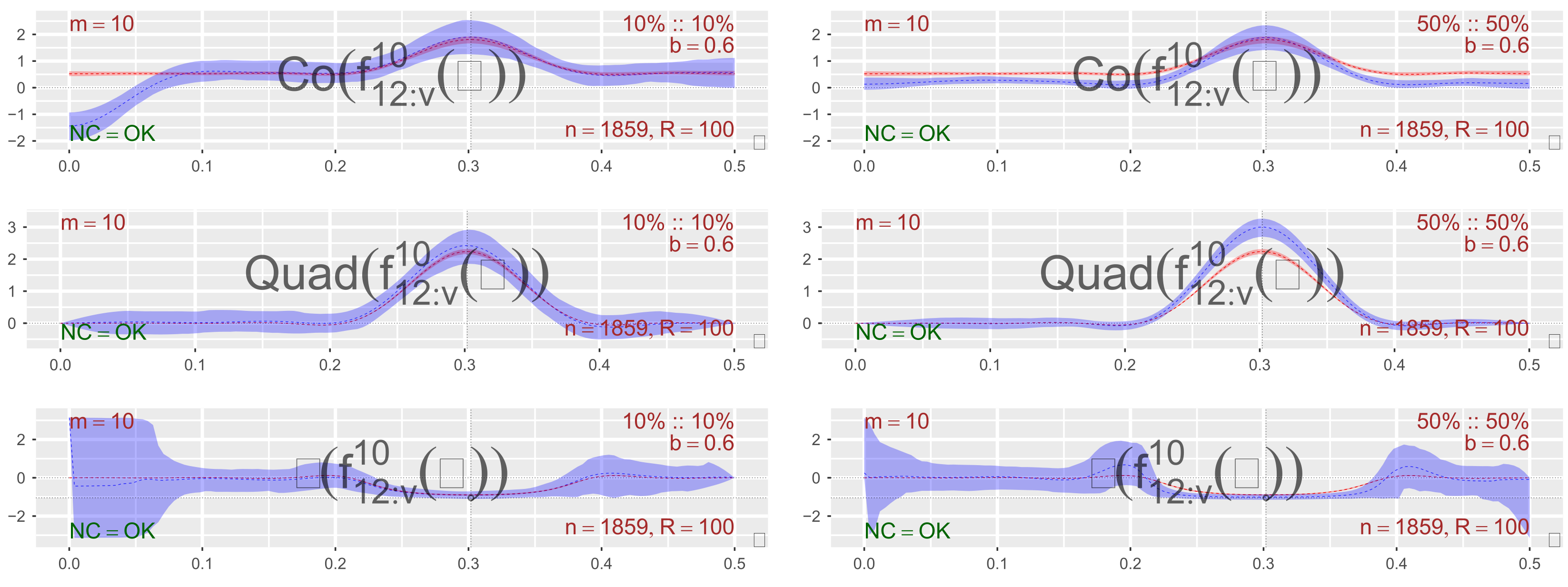
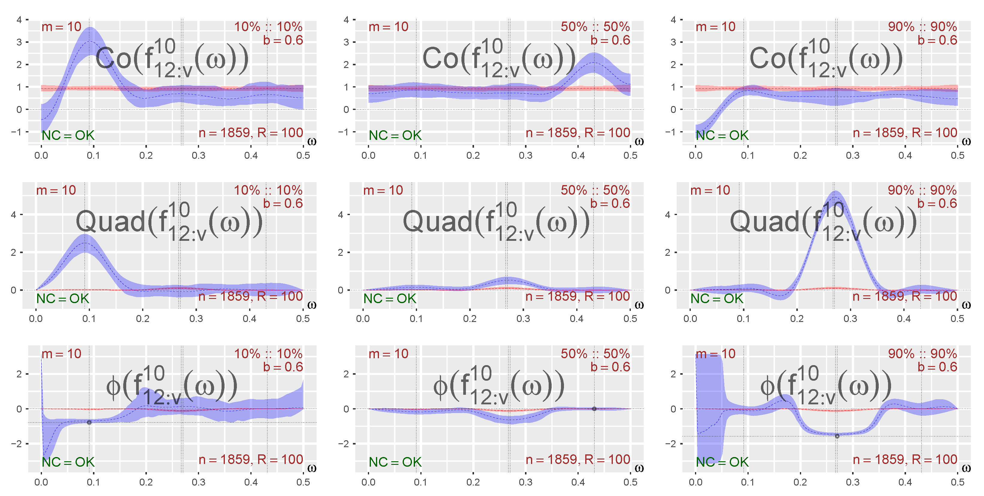
where is Gaussian white noise with mean zero and standard deviation , with and independent, and where, in addition, it is such that and are fixed for all the replicates, whereas is drawn uniformly from for each individual replicate. A realization with , , and is used for the Co-, Quad-, and Phase-plots shown in Figure 1, where 100 independent samples of length 1859 were used to obtain the estimates of the m-truncated spectra and their corresponding 90% pointwise confidence intervals (based on the bandwidth ). Some useful remarks can be based on this plot, before the bivariate local trigonometric case is defined and investigated.
In this particular case, the local Gaussian spectra (in blue)5 in Figure 1 shares many similarities with the corresponding global spectra (in red).6 In particular, the peaks of the Co- and Quad-plots lie, for both the local and global spectra, at the frequency (shown in the plots as a vertical line), and the corresponding Phase-plots at this frequency lie quite close to the phase adjustment (shown as a horizontal line, positioned with an appropriate sign adjustment). This phenomenon is present both for the point at 10%::10% and the point at 50%::50%, i.e., the local information at these quantiles is sufficient to pick up both the spectral peak and the phase adjustment expected from the global model. However, it should be noted that this nice match does not hold for all values of . In fact, experiments with different values for (plots not included in this paper) indicate that the difference between the local and global spectra becomes larger (in particular for the point 10%::10%) when becomes smaller. See JT22 [Appendix G.4.4] for some further comments related to this issue.
Note that the wide pointwise confidence band observed for near 0 in the 10%::10%-Phase-plot in Figure 1 is related to the branch-cut that occurs at in the definition of the phase-spectrum, cf. Definition 2. The simple algorithm used for the creation of the pointwise confidence intervals was not tweaked to properly cover the case where the majority of the estimates lie in the second and third quadrants of the complex plane, which implies that the Co- and Quad-plots should be consulted instead when the Phase-plot misbehaves in this manner.
The values of the Co- and Quad-plots (for a given frequency ) are (for each frequency) related to the corresponding values of the Amplitude- and Phase-plots by the following simple relations:
which follows trivially from the way these spectra are defined relative to Cartesian or polar representations of the complex-valued cross-spectra, cf. Equation (3) and Definition 2. For the example investigated in Figure 1, where the Phase plot is close to at , it thus follows that the peak for the Quad-spectrum should be approximately times larger than the peak of the Co-spectrum.
The plots encountered later in this paper will be based on the abovementioned Cartesian or polar representations of , but it is, in principle, also possible to make plots (and animations) that, for a given value of , show the estimated values of as point clouds in the complex plane. A discussion related to this complex-valued plot approach is given in Section S6.4 in the Supplementary Material (see, in particular, Figure S6.2).
The bivariate local trigonometric case: Two bivariate extensions of the artificial local trigonometric time series from JT22 [Section 3.3.2] are now considered. The key idea is that an artificial bivariate time series can be constructed by the following scheme:
- Select bivariate time series .
- Select a random variable I with values in the set , and use this to sample a collection of indices (that is, for each t, an independent realization of I is taken). Let denote the probabilities for the different outcomes.
- Define by means of the equationThe indicator function 𝟙{·} ensures that only one of the bivariate -components contributes for a given value t, that is, it is also possible to write .
The bivariate local trigonometric time series (needed for the sanity testing of the implemented estimation algorithm) can now be constructed by selecting r cosine-functions that oscillate around different horizontal baselines , that is,
where , and , respectively, represent frequency and phase adjustments occurring in the cosine-function, and where the amplitudes are uniformly distributed in some interval . Note that it is assumed that the phases are uniformly drawn (one time for each realization) from the interval between 0 and , whereas the phases are constants. It is also assumed that the stochastic processes , and are independent of each other.
The auto- and cross-correlations of , as given by Equations (22) and (23), are functions of and . The auto-correlations of the marginal time series were computed in JT22 [Appendix G.4], and the corresponding result for the cross-correlation is given in Section S6.5 in the Supplementary Material. For the purpose of the present section, it is sufficient to know that it is possible to find parameter configurations for which the global spectrum (based on the pseudo-normalized observations) is rather flat (when truncated at ), which implies that it cannot detect the frequencies of the underlying structure. As will be seen in the ensuing simulation experiments, the randomly sampled information for the local versions and of Equation (23) may still be sufficient to recover the local periodic and phase structure.
Note that neither nor are well defined for the bivariate local trigonometric times series, but this is not important since it still is possible to predict (cf. Section S6.5 for details) that the m-truncated estimates for some points (and a given bandwidth ) should resemble Figure 1—and this can be used, cf. Figures 3 and 5, to test the sanity of the implemented estimation algorithm. These plots also reveal that the local Gaussian versions of the Co-, Quad-, and Phase-plots can detect local properties that are undetected by the ordinary version of these spectra.
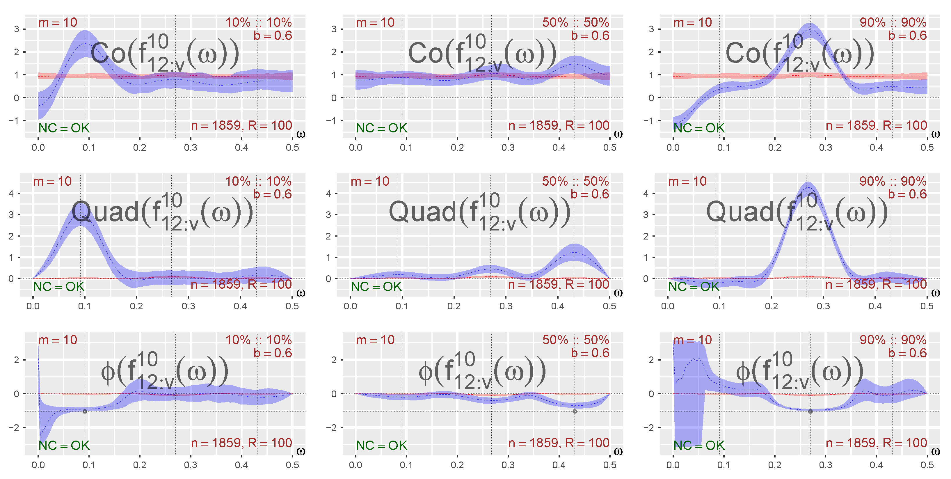
Parameter setup: The models for the two time series presented in this section are based on an extension of the univariate case seen in JT22, that is, both have components, the probabilities are given by , the frequencies are given by , the baselines are given by the values , and the lower and upper ranges for the uniforms sampling of the amplitudes are, respectively, given by and . Note that and should be selected in order to give a minimal amount of overlap between the different components, cf. Section S6.5 for further details.
The distinction between the two models is due to the selection of the additional phase adjustments . The model investigated in Figure 2 and Figure 3 has a constant phase adjustment of , whereas the model investigated in Figure 4 and Figure 5 has individual phase adjustments, given as .
To complete the specification of the setup, note that the 90% pointwise confidence intervals in Figure 3 and Figure 5 all are based on 100 independent samples of length 1859 from the above-described models, and that the bandwidth was used in the computation of the local Gaussian cross-correlations.
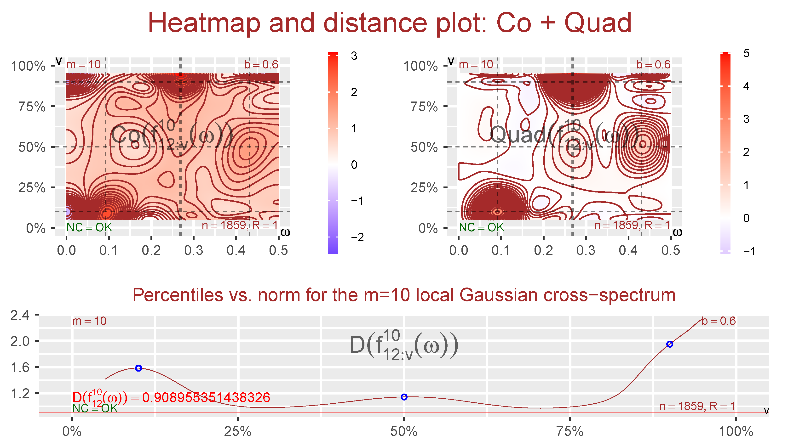
Constant phase adjustment: The case where the phase difference was used for all the is investigated in Figure 2 and Figure 3. This particular example was created in order to test the sanity of the estimation algorithm. The resulting bivariate sample will, by construction, cf. Section S6.5.1 for details, have an ordinary cross-spectrum that looks quite flat (not possible to extract any useful information). Furthermore, cf. the last sentence of the paragraph following the one containing Equation (23), and the heuristic argument given in Section S6.5.2, it is possible to find configurations of bandwidth and point for which the resulting local Gaussian spectra should look a bit similar to those encountered in Figure 1 for the three designated points, 10%::10%, 50%::50%, and 90%::90% (which turns out to be the case, cf. Figure 3).
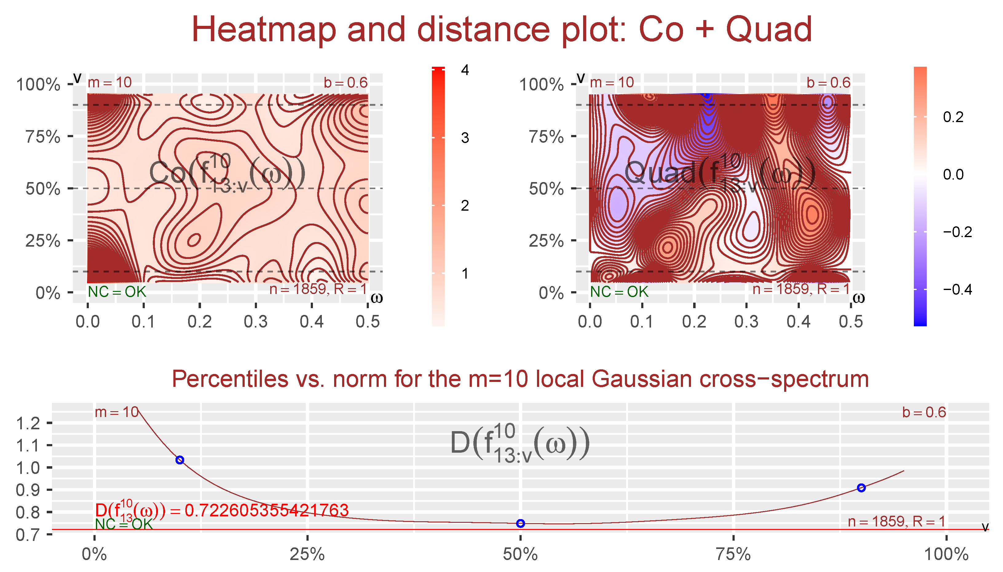
It will, in general, not be known in advance for which points of that local features might be present, and it is thus necessary to use a strategy that can help identify interesting regions. For this purpose, an adjusted version of the combined heatmap and distance plots introduced in JT22 will be used, as seen in Figure 2, where the point varies along the diagonal. The heatmap part of the plot must be adjusted a bit since the estimated m-truncated local Gaussian cross-spectrum is a complex-valued entity, and the solution seen in Figure 2 shows a decomposition into the Co- and Quad-plots. The distance parts of these plots are based on the distance function D that is inherited from the complex Hilbert space of Fourier series on the interval , cf. Section S3.1 for further details. The distance plot can help an investigator see how far the time series of interest is from being i.i.d. observations—and it enables a comparison with the global spectrum that is not possible based only on the heatmap plots.
Note that the heatmap part of the plots can also be based on a polar decomposition into Amplitude- and Phase-plots, but it is easier to digest the information from the Co- and Quad-plots. It is, e.g., easy to see that different local structures are present in the samples investigated by Co- and Quad-based heatmaps in Figure 2 and Figure 4, but this difference is not that clear when Amplitude- and Phase-plots are used instead, cf. Section S3.2.2 for further details.
Keep in mind that the pseudo-normalization step in Algorithm 1 implies that the plots related to only reveal information about the cross-temporal interdependency structures of the sample. An investigator must thus use some supplementing technique in order to extract information from the marginal distributions.
The contours in the heatmap plots seen in Figure 2 reveal that different peaks occur at different combinations of points and frequencies , in agreement with the heuristic argument that motivated the construction of this example. Together with the distance plot part, which shows how much the m-truncated local Gaussian cross-spectrum differs from the corresponding m-truncated ordinary cross-spectrum, this shows that it could be of interest to take a closer look at the three points investigated in Figure 3.
The three points investigated in Figure 3 correspond to the function components in Equation (23) with indices . The point that corresponds to the component would, due to the combination of the low probability and the placement of the level , lie too far out in the tail to be properly investigated by the present sample size. Note that the component is included here in order to show that an exploratory approach based on local Gaussian spectra can fail to detect local signals that are much weaker than the dominating ones, cf. the discussion in Section S6.5.
For the points investigated in Figure 3, it seems to be the case that the local Gaussian parts of the Co-, Quad-, and Phase-plots together reveal local properties in accordance with the outcome expected from the knowledge of the generating model—and these local structures are not detected by the ordinary global spectra, which in this case (due to the values used for and ) are quite close to being flat (i.e., information about the specified frequencies cannot be extracted from the global spectrum, cf. Section S6.5.1). The left column investigates a point at the lower tail of the diagonal, and it can there be observed that both the Co- and Quad-plots have a peak close to the leftmost -value—and the value of the corresponding Phase-plot for frequencies close to this -value lies quite close to the phase difference between the first and second component. A similar situation is present for the three plots shown in the right column, where a point at the upper tail of the diagonal is investigated. Moreover, in accordance with the general discussion related to Equation (21), the peaks of the Quad-plots are higher than those of the Co-plots in this case due to the phase difference that was used in the input parameters.
For the center column of Figure 3, which investigates the point at the center of the diagonal, it can be seen that the Quad- and Phase-plots, in addition to the expected -value, also detect the presence of the other -values. The Phase-plot is, for this point, not that close to the expected value, but that situation changes if the truncation is performed at a higher lag than . The center column thus shows the importance of considering a range of values for the truncation level when such plots are investigated. The additional peaks that are detected in the center column are due to contamination from the neighboring regions.
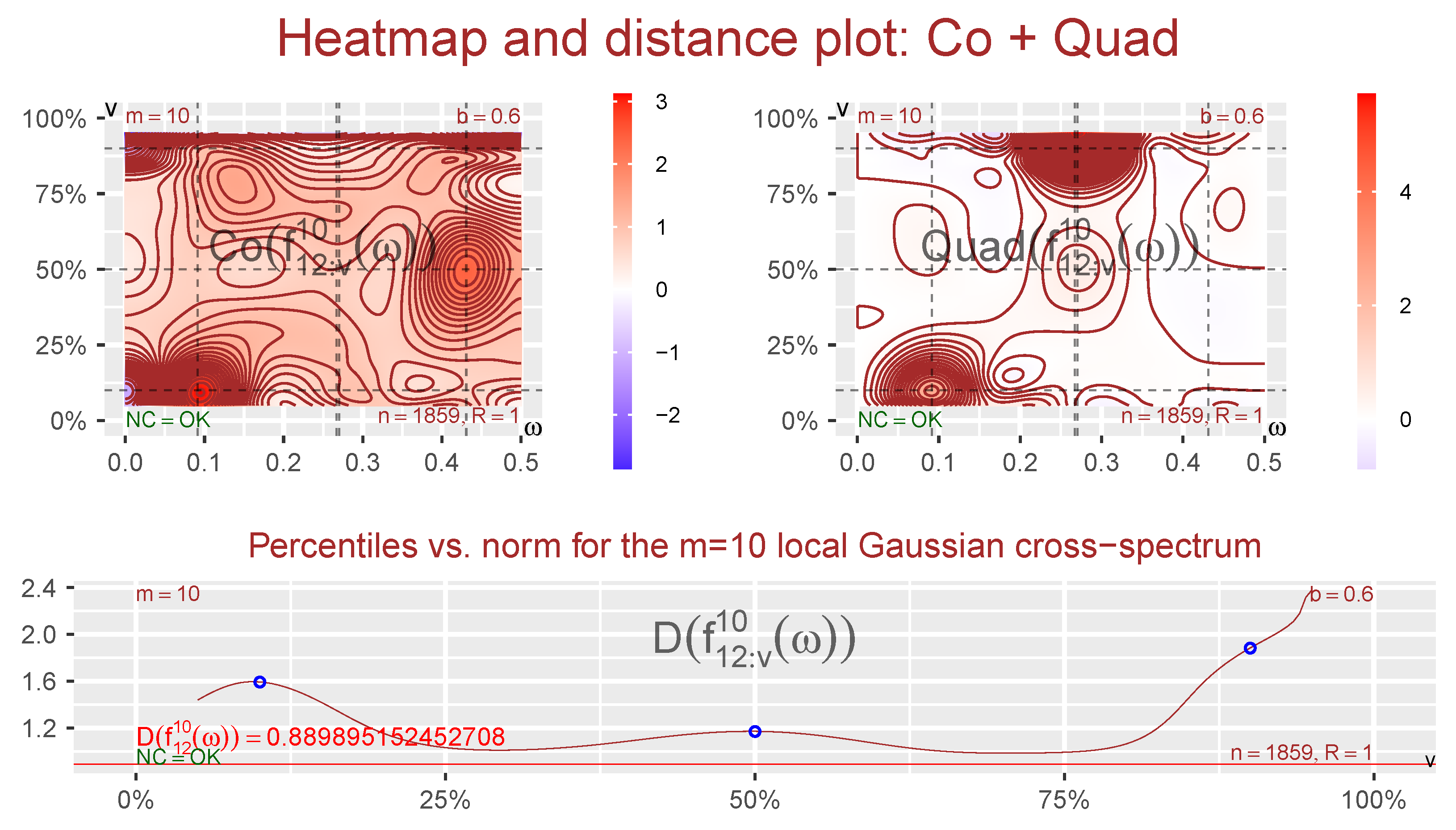
Individual phase adjustment: The phase-spectrum contains information about the lead–lag relationship between two time series. In practice, it is conceivable, as indicated in the third paragraph of the Introduction, that the lead–lag relationships are different at extremes; i.e., in the distributional tails, compared to in the center of the series. In fact, such a difference is indicated in the lower row of Figure 9 of the DAX–CAC index pair to be treated in Section 3.2.1 It is therefore of interest to examine the potential of the local Gaussian analysis to pick up such differences for the bivariate local trigonometric example. We therefore regenerated this example with the following individual phase adjustments: . The heatmap and distance plot seen in Figure 4 reveals, once more, in agreement with the way the example was constructed, that it is natural to look at the three points shown in Figure 5. The horizontal lines seen in the Phase-plots part of Figure 5 show the -values (adjusted to have the correct sign), and for each of the designated points, the intersection with the relevant vertical -line is highlighted to show the expected outcome based on the knowledge of the model.
The Co-, Quad-, and Phase-plots in Figure 5 behave in accordance with what was observed in Figure 3; in particular, the Phase-plots pick up the individual phase adjustments, giving values that lie close to the expected -value when the frequency is near the corresponding -value. However, there are also changes in the Co- and Quad-spectral plots that can be explained. In fact, the height of the corresponding Co- and Quad-peaks are in accordance with the values of the Phase-plots. In particular, the phase-adjustment is for the point 10%::10%, which implies that the Co- and Quad-peaks should rise approximately to the same height above their respective baselines, which seems to be fairly close to the observed result. For the points 50%::50% and 90%::90%, the situation is clearer since the respective local frequencies and then imply that only the Co-plot should have a peak for the point 50%::50% and only the Quad-plot should have a peak for the point 90%::90%, again in agreement with the impression based on Figure 5. The global spectrum in Figure 5 (red line) does not reveal any of this local spectral structure.
The examples investigated in Figure 1, Figure 2, Figure 3, Figure 4 and Figure 5 do not satisfy the requirements needed for the asymptotic results (both for the global and local cases) to hold true; in particular, the local Gaussian cross-correlations will, in these cases, not be absolutely summable.7 Despite this, the examples are still of interest since they show that an exploratory tool based on the local Gaussian spectra in this case (with a truncation at ) can detect information that is in agreement with what could be expected based on the parameters used in the models for .
The underlying model will, of course, not be known when a real multivariate time series is encountered, so it is important to estimate the local Gaussian cross-spectrum at a wide range of points in the plane and a wide range of truncation levels m. This kind of investigation can be performed using the heatmap and distance plots seen in Figure 2, Figure 4 and Figure 7.
Even when it might not be obvious how to interpret the results shown in the Co-, Quad-, and Phase-plots, it should be noted that they can be used as an exploratory tool that can detect nonlinear traits in the observations. Moreover, these plots can also be used to investigate if a model fitted to the data contains elements that can mimic the observed features. The recipe for this approach would then be to first select a model, then estimate parameters based on the available sample, and finally use the resulting fitted model to generate independent samples of the same length as the sample. Section 3.2 will show an example of this approach, cf. Figures 9 and 12. Further details related to this are given in Section S5.1.
3.2. A Real Multivariate Time Series and a Poorly Fitted GARCH-Type Model
This section will show how the Co-, Quad-, and Phase-plots can be used as an exploratory tool on a financial dataset, and then it will be seen how this approach also can be used to obtain a visual impression of the quality of a multivariate GARCH-type model fitted to these data. The multivariate time series sample to be considered in this section will be a bivariate subset of the (log-returns of the) tetravariate EuStockMarkets-sample from the datasets-package of R, R Core Team (2020). This dataset was selected since it has a length that should be large enough to justify the assumption that the observed features in the Co-, Quad-, and Phase-plots are not solely there due to small sample variation.
The EuStockMarkets contains 1860 daily closing prices collected in the period 1991–1998, from the following four major European stock indices: Germany DAX (Ibis), Switzerland SMI, France CAC, and UK FTSE. The data were sampled in business time, i.e., weekends and holidays were omitted. The log-returns of the EuStockMarkets values gives a dataset that seems natural to model with some multivariate GARCH-type model, and the R-package rmgarch, Ghalanos (2022a), was used for that purpose. Note that the present paper only aims to show how this kind of analysis can be performed, so only one very simple model was investigated—which thus gave a rather poor model for the data at hand.
The local Gaussian approach presented here is based on a pseudo-normalization of the marginal distributions. It is thus, in essence, properties of the copula structures of the time series that are revealed here, and a practitioner should supplement this approach by methods that also extract information from the original marginals.
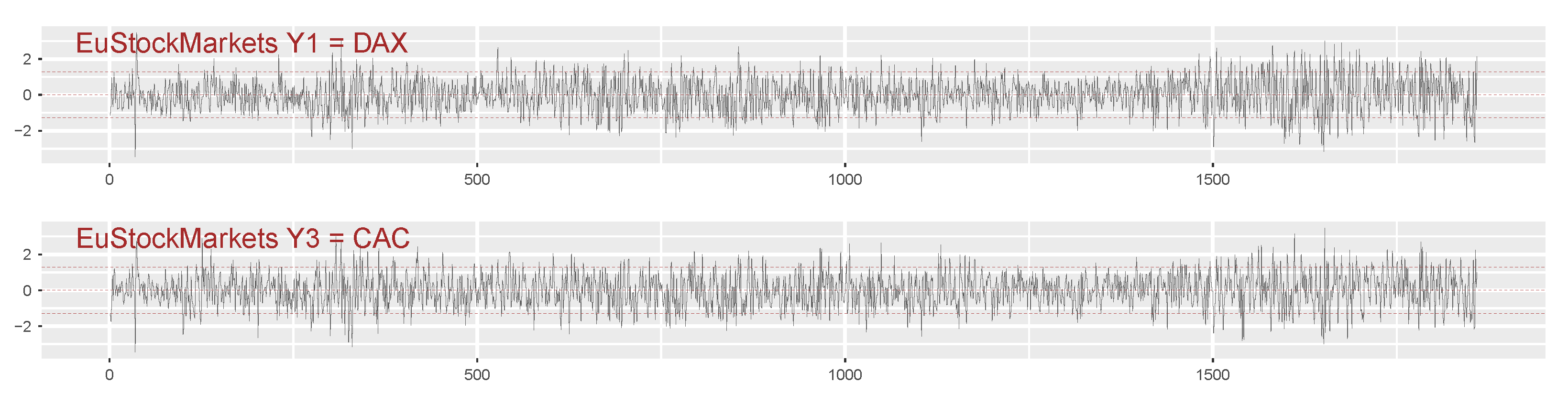
3.2.1. The DAX–CAC Subset of the EuStockMarkets-Log-Returns
The log-returns of the bivariate EuStockMarkets-subset , of length 1859, will now be investigated.8 The individual pseudo-normalized traces of these observations are shown in Figure 6, and it will be from these pseudo-normalized observations that the local Gaussian cross-correlations will be computed.
A local Gaussian investigation requires that some points must be selected, and thereafter an in-depth investigation can be performed for the selected points. The heatmap and distance plots can be useful for the task of identifying interesting points along the diagonal, as seen in the Figure 7, where the truncated Co- and Quad-spectra are presented for the DAX- and CAC-components of the log-returns of the EuStockMarkets-data.
The scale indicators for the heatmap plots in Figure 7 reveal that it is the Co-spectrum that dominates, and it is clear that the situation in the tails is different from the one in the center. The asymmetry between the upper and lower tail is not immediately visible from the heatmap part of Figure 7, but it is easy to see from the distance part of the plot that the local Gaussian interdependency structure is stronger in the lower tail.
From the information in Figure 7, it can now be seen that it could be of interest to compare the behavior in the tails with that at the center. The selected points are highlighted in Figure 7 with the help of added lines (the heatmap part) and circles (the distance part). These points are the same as those used for Figure 3 and Figure 5, i.e., the diagonal points whose coordinates correspond to the 10%, 50%, and 90% percentiles of the standard normal distribution.
The estimates of the local Gaussian cross-correlations might degenerate toward or if the points are too far out in the tails. It is thus of interest to check the behavior of these estimates for the given sample before the computationally costly production of pointwise confidence intervals (based on resampling) is undertaken. The result of this investigation of the estimated local Gaussian cross-correlations is seen in Figure 8, where a wide range of values for h is included. The observed values of indicate that degeneration of the estimates are not a problem for these points.
It seems to be the case that the local Gaussian spectrum can detect nonlinear structures even with a rather low truncation level m, but the value used in this paper is solely selected in order to present a proof-of-principle. For an actual investigation it would be natural to investigate a wider range of different lags h, such as those seen in Figure 8, in order to check what kind of behavior is observed. The interested reader will find a sensitivity analysis of m in Section S3.4, which is based on the values seen in Figure 8.
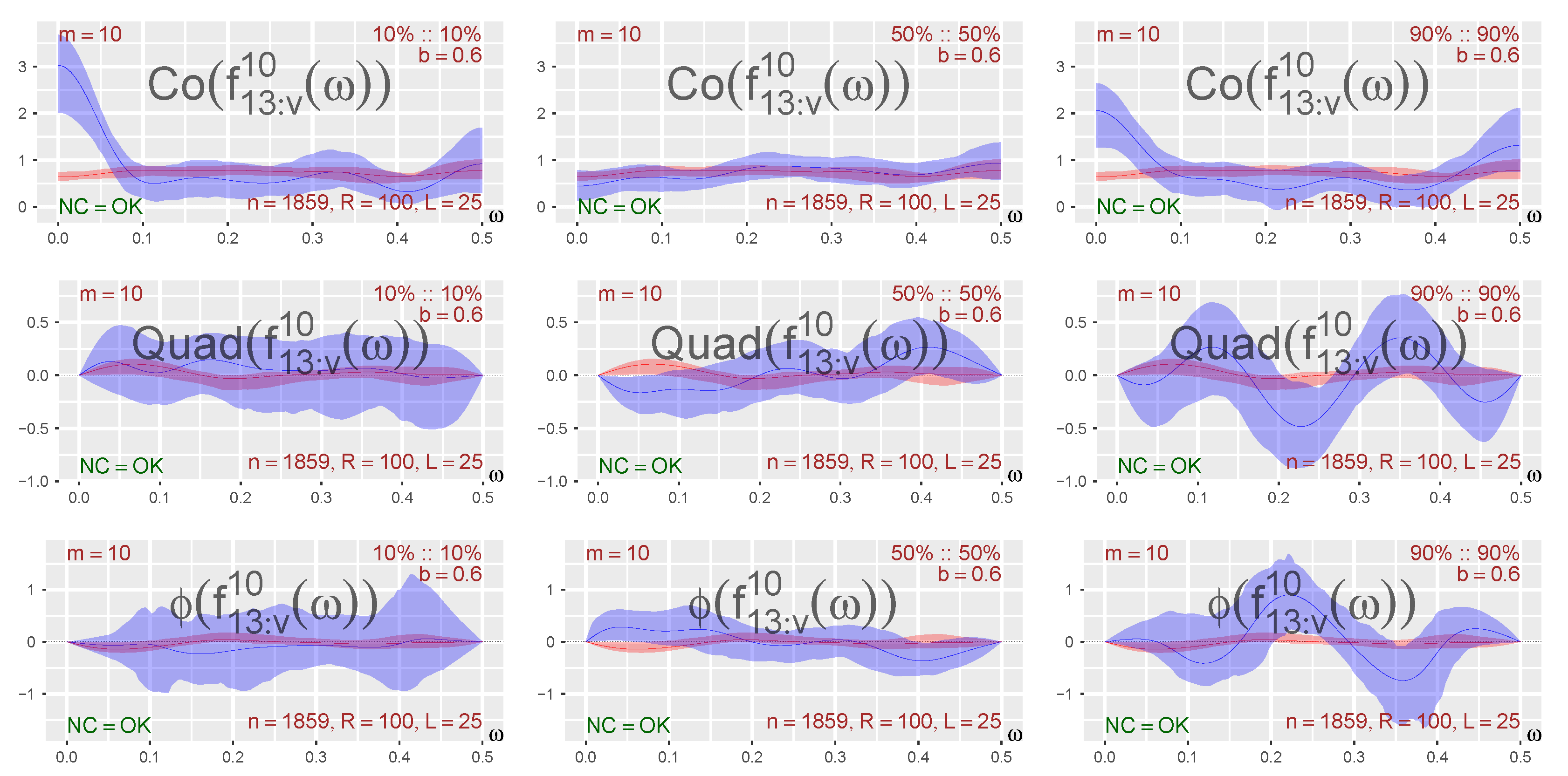
Figure 9 shows the Co-, Quad-, and Phase-spectra obtained from the truncated global and local spectra for the three selected diagonal points. A solid red line represents the estimate of the ordinary cross-spectrum , whereas a solid blue line represents the estimate of the local Gaussian cross-spectrum . The 90% pointwise confidence intervals were created based on block-bootstrap replicates using a block length of for the circular-index-based block bootstrap for tuples resampling strategy developed in JT22. Details related to this resampling strategy are given in Section S5 in the Supplementary Material, and the sensitivity analysis in Section S5.3 reveals that the results in this case are stable over a wide range of block lengths.
The three points considered in Figure 9 all lie on the diagonal, since it seems easier to give an interpretation for those points. In particular, the point 10%::10% represents a situation where the market moves down both in Germany and France, whereas the points 50%::50% and 90%::90% similarly represent cases where the market either is stable or moves up in both countries. For the purpose of the present paper, it suffices to point out that the Co-, Quad-, and Phase-plots of Figure 9 indicate that the data contain nonlinear traits, which in particular is visible in the Co-plot for the point 10%::10% and for all the plots related to the point 90%::90%. It should be noted that the Co-plots at the frequency simply give a weighted sum of the local Gaussian cross-correlations (between ) seen in Figure 8, so the Co-plot peaks at for the points 10%::10% and 90%::90% are thus as expected, and the lack of a Co-plot peak at for the point 50%::50% also seems natural in view of Figure 8. It should also be noted that the peak for the 90%::90% Co-plot is lower than the corresponding peak for 10%::10%, but this seems, in this case, to be due to the low truncation level used for the plots, i.e., these two peaks attain approximately the same height when a higher truncation level is applied.
It seems, for the particular parameter configuration that generated the plots in Figure 9, to be the case that the point 90%::90% has the most interesting Quad- and Phase-plots, but again, as noted above, it may be premature to place too much emphasis on this particular plot given the uncertainties involved in the selection of the bandwidth and the truncation level m. As mentioned before, the effects of changes to the block length L, are quite minimal, cf. the discussion in Section S5.3, in the Supplementary Material.
It should also be noted that a low number of bootstrapped replicates can be a source of small sample variation for the width of the estimated pointwise confidence intervals, and this is important to keep in mind if a minor gap is observed between the pointwise confidence intervals for the local and global spectra. Such gaps could appear or disappear when the algorithm is used to generate new computations based on the same number of bootstrapped replicates, a behavior that, in particular, has been observed for the rightmost peak/trough of the Quad- and Phase-plots at the point 90%::90% in Figure 9. This kind of ambiguity can be countered by increasing the number of bootstrapped replicates, but that was not carried out for the present example due to the increased computational cost.
The peak at the center of the 90%::90% Phase-plot in Figure 9 seems to be significantly different from the global spectrum, which strengthens the impression that something of interest might be present at that frequency. However, it is important to keep in mind that this impression is based on the present combination of bandwidth and truncation level—and there are, at the moment, no data-driven methods for the selection of these parameters. (A positive phase difference is consistent with the 90%::90% cross-correlation plot in Figure 8, which might indicate that the DAX is leading over CAC when the market is going up. We were not able to find similar evidence in the ordinary spectrum-based literature, but there are other methods for determining lead–lag relationships using comparisons in terms of intensity of jumps of the two series involved, cf. Eyjolfsson and Tjøstheim (2023) for the index pair S&P 500 and Nikkei 225, and Aït-Sahalia et al. (2015) in their investigation of financial contagion.)
Note that the shiny-interface in the R-package localgaussSpec should be used if it is of interest to pursue a further analysis of the local Gaussian spectra of the log-returns of the EuStockMarkets-data, since that enables an interactive investigation that shows how the estimates vary based on different bandwidths and truncation levels m. Moreover, as discussed in Section S5.3, it is also possible to check how the selection of the block length L for the bootstrap procedure developed in JT22 influences the widths of the pointwise confidence intervals in the Co-, Quad-, and Phase-plots.
3.2.2. A Simple Copula-GARCH-Model Fitted to the EuStockMarkets Log-Returns
It might not be obvious how to interpret the Co-, Quad-, and Phase spectra based on the log-returns of the EuStockMarkets-data, but they do at least provide an approach where nonlinear dependencies might be detected from a visual inspection of the plots.
Furthermore, it is possible to use this as an exploratory tool in order to investigate whether a model fitted to the original data is capable of reproducing nonlinear traits that match those observed for the data. The procedure is straightforward:
- Fit the selected model to the data.
- Perform a local Gaussian spectrum investigation based on simulated samples from the fitted model. The parameters should match those used in the investigation of the original data.
- Compare the plots based on the original data with corresponding plots based on the simulated data from the model. It can be of interest to not only compare the Co-, Quad-, and Phase-plots, but also include plots that show the traces and the estimated local Gaussian auto- and cross-spectra.
For the present case of interest, Item 2 of the list above implies that 100 independent samples of length 1859 will be used as the basis for the construction of the Co-, Quad-, and Phase-plots of the fitted model, and the bandwidth will be used for the estimation of the local Gaussian cross-correlations at the three diagonal points 10%::10%, 50%::50%, and 90%::90%.
The model: The R-package rmgarch was used to fit a simple multivariate GARCH-type model to the log-returns of the EuStockMarkets-data, in order to exemplify the procedure outlined above, i.e., a copula-GARCH-model (cGARCH) with the simplest available univariate models for the marginals9 was fitted to the data, and the resulting model was then used to produce Figure 10, Figure 11 and Figure 12. See Section S6.3 for further details. Note that this simple model was selected simply in order to provide a proof-of-principle example for the investigations encountered later on. It was, in particular, of interest, as discussed in Section S5.1, to use a “too-simple model” in order to highlight the ideas related to the local Gaussian sanity testing of parametric models fitted to a sample.
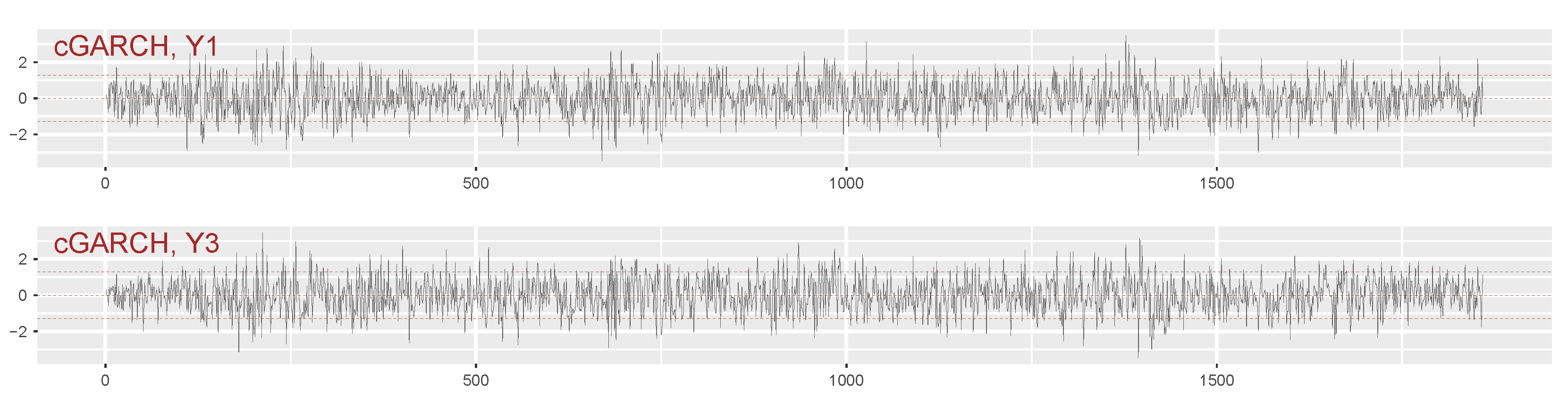
The traces: Figure 10 shows the pseudo-normalized trace of the - and -variables for one sample from the tetravariate cGARCH-model, and this can be compared with the corresponding pseudo-normalized trace of the DAX and CAC plot for the pseudo-normalized log-returns of the EuStockMarkets-data (see Figure 6). Obviously, a comparison of one single simulated trace with the trace of the original data might not reveal much, and it should also be noted that it, in general, might be preferable to compare the traces before they are subjected to the pseudo-normalization, since that could detect if the model might fail to produce sufficiently extreme outliers.
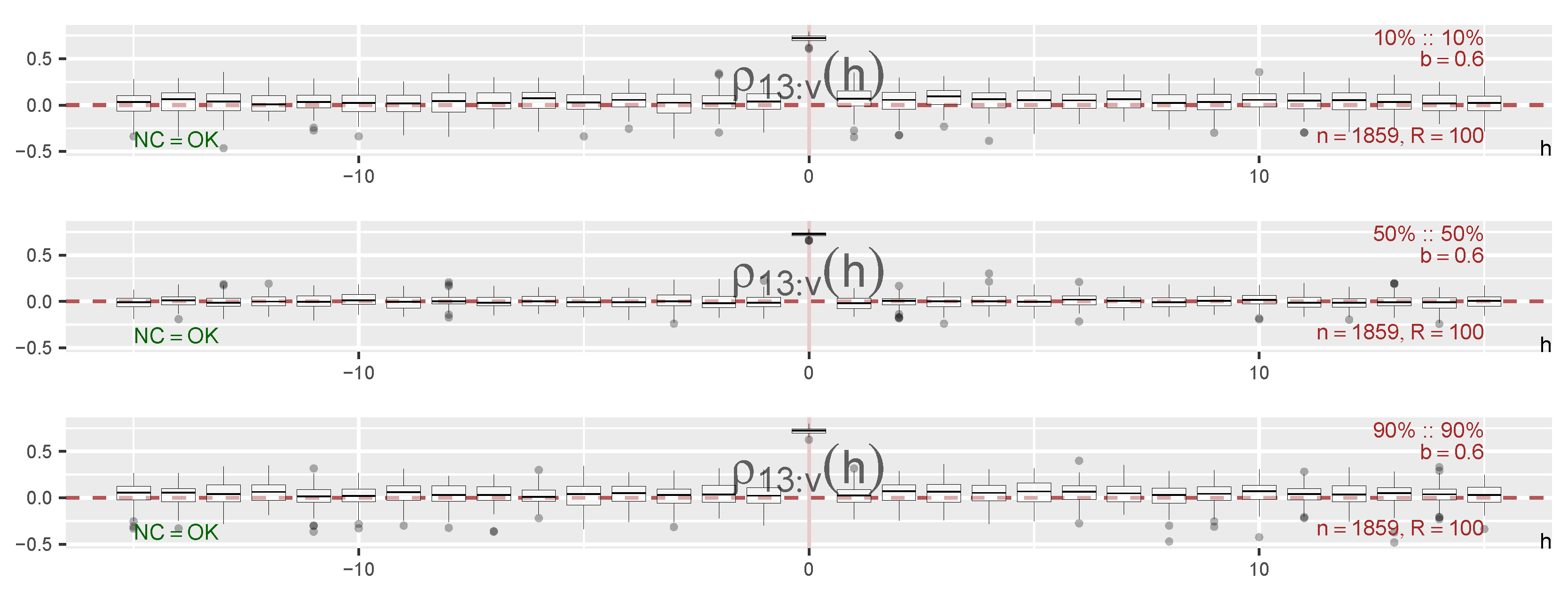
The local Gaussian correlations: Boxplots, based on the 100 independent estimates of the local Gaussian cross-correlations from the cGARCH-model, are shown in Figure 11. These can be compared with the local Gaussian cross-correlations estimated from the original sample, shown in Figure 8. It should be noted that the computational cost for the production of the boxplots in Figure 11 is substantially larger than the cost for the production of the simpler plots shown in Figure 8, so it is preferable to restrict the attention to a shorter range of lags in Figure 11. Note also that the wide range of lags included in Figure 8 is related to the desire for an initial investigation of the sensitivity of the truncation level m, and it is, as seen here, possible to judge the suitability of the fitted model from the shorter range of lags included in Figure 11.
The impression from the lags included in Figure 11 is that the medians of the estimated local Gaussian cross-correlations for the point 50%::50% are quite close to zero, whereas the medians for the points 10%::10% and 90%::90% are mostly slightly above zero. Almost none of the boxes for the two latter points appear to be positioned in a manner consistent with the desired outcome for a good match with the corresponding estimated values in Figure 8, and it might thus be ample reason to suspect that this cGARCH-model might better be replaced with another model instead.
The Co- Quad-, and Phase-plots: Figure 12 shows the local Gaussian spectra for the same points and the same configuration of parameters as those used in Figure 9.
The Co-, Quad-, and Phase-plots of Figure 12 look as if they could originate from i.i.d. white noise—which comes as no surprise in view of the information about the local Gaussian cross-correlations in Figure 11. The Co-plots for the two points 10%::10% and 90%::90% show that the estimates of the m-truncated local Gaussian co-spectra, i.e., the blue dashed lines, might have a peak at —but the 90% pointwise confidence intervals are too wide to support a claim that these peaks are significant. A further comparison of these two Co-plots with the corresponding Co-plots in Figure 9 (beware of different scales for the axes) shows that the confidence intervals from Figure 12 are too narrow (at ) to encompass the peaks observed in Figure 9—which indicates that the selected model might be a rather bad approximation to the log-returns of the EuStockMarkets-data. It thus seems advisable to look for some other model instead, a natural conclusion given that no effort whatsoever was made with regard to finding reasonable marginal distributions for the copula-GARCH-model used in this discussion.
It should be noted that a local Gaussian spectra comparison of the original data and the fitted model in practice also should include a comparison of the local Gaussian auto-spectra of the marginals, as was performed in JT22. These auto-spectra plots (not included in this paper, but see Section S3.2.1 for some related heatmap and distance plots) can provide some additional information useful for the model selection process. In particular, if a model selection algorithm for GARCH-type models is used to pick one marginal model from a given collection of marginal models, then an investigation based on the local Gaussian auto-spectrum might reveal if the selected marginal model captures the local traits of the corresponding marginal observations in a reasonable manner.
The preceding discussion was restricted to three diagonal points, but the local Gaussian sanity testing of a fitted parametric model can also be performed for points outside of the diagonal. Such an approach was discussed for the univariate case in JT22 [Appendix F.2], and a natural extension to the multivariate case is presented in Section S5.1 in the online Supplementary Material.
4. Conclusions
The local Gaussian auto-spectrum from JT22 can, as seen in this paper, be extended to cover the multivariate case, too—and estimates of the m-truncated local Gaussian cross-spectrum can be used to detect nonlinear cross-temporal dependencies between the marginals and of a multivariate time series .
The resulting local Gaussian approach to spectral analysis can, in particular, be used to detect if the interdependency structure of the time series under investigation deviates from being Gaussian. For time series whose ordinary auto- and cross-spectra are flat, any peaks and troughs from the local Gaussian approach can then be considered indicators of local nonlinear traits and local periodicities.
The m-truncated estimates can, as discussed for GARCH-models in Section 3.2, also be of interest with regard to local comparisons of models fitted to a given sample. In particular, it is possible to use this approach to check if a model fitted to the data can reproduce local traits detected in the original sample, and an investigator can thus use a local Gaussian sanity test of the fitted models as a supplement to other model selection methods.
All the examples in this paper can be reproduced with the help of the scripts that are included as a part of the R-package localgaussSpec. The interested reader can run these scripts, and then use the integrated shiny-application from this R-package to investigate how the resulting plots change when the tuning parameters in the estimation algorithm are modified. This enables a much deeper inspection of the results than the static plots contained in this paper. These scripts can also be used as templates for new investigations, and they can hopefully help any interested readers to test out the local Gaussian approach to spectral analysis on their own data.
Supplementary Materials
The following supporting information can be downloaded at: https://www.mdpi.com/article/10.3390/econometrics11020012/s1. The online Supplementary Material, contains the proofs of the theoretical results, discussions related to the sensitivity of the different input parameters in the estimation algorithm, and also a discussion of the sensitivity of the block length in the bootstrapped-based resampling algorithm that was developed in JT22 for the local Gaussian spectral investigation. The Supplementary Material also contains a discussion related to how the local Gaussian spectra (based on samples) of a parametric model can be compared to the local Gaussian spectra from the sample the model was fitted to. The reproduction of all the results in this paper can be achieved with the help of the scripts contained in the R-package localgaussSpec,10 and details about this are also available in the Supplementary Material. The Supplementary Material ends with a discussion related to the construction of the test data used for the sanity testing of the estimation algorithm, and this part also highlights some limitations that a practitioner should keep in mind when the local Gaussian approach is used in the extreme tails of the sample at hand. Note that the references Birr et al. (2019); Bollerslev and Ghysels (1996); Brockwell and Davis (1986); Ghalanos (2022b); Klimko and Nelson (1978); Künsch (1989); Politis and Romano (1992) are cited in the Supplementary Material.
Author Contributions
Conceptualization, L.A.J. and D.T.; methodology, L.A.J. and D.T.; software, L.A.J.; validation, L.A.J.; formal analysis, L.A.J. and D.T.; investigation, L.A.J. and D.T.; writing—original draft preparation, L.A.J.; writing—review and editing, L.A.J. and D.T.; visualization, L.A.J. and D.T.; supervision, D.T. All authors have read and agreed to the published version of the manuscript.
Funding
This research received no external funding.
Institutional Review Board Statement
Not applicable.
Informed Consent Statement
Not applicable.
Data Availability Statement
The EuStockMarkets-dataset is a part of the datasets-package of R, R Core Team (2020). The scripts needed for the reproduction of the examples in this paper is contained in the R-package localgaussSpec, cf. Section S6.1 for further details.
Acknowledgments
The authors are most grateful for the valuable comments and suggestions from the referees and the associate editor.
Conflicts of Interest
The authors declare no conflict of interest.
| 1 | This multivariate approach was initiated in the first author’s Ph.D. thesis, available at https://bora.uib.no/handle/1956/16950. The version in this paper has been extended with new methods and visualizations that were developed due to review comments related to the univariate theory published in JT22. |
| 2 | This is due to the way the local Gaussian correlation is defined; see Tjøstheim and Hufthammer (2013) for details. |
| 3 | The corresponding coordinates are , , and . |
| 4 | The Amplitude-plots are not included here since the interesting details (in most cases) would already have been detected by the other plots. |
| 5 | If you have a black and white copy of this paper, then read “blue” as “light” and “red” as “dark”. |
| 6 | The dotted lines represent the means of the estimated values, whereas the 90% pointwise confidence intervals are based on the 5% and 95% quantiles of these samples. |
| 7 | In this respect, the situation is similar to the detection of a pure sinusoidal for the global spectrum. |
| 8 | The corresponding script in the R-package localgaussSpec enables an investigation of all the combinations between DAX, SMI, CAC, and FTSE, but only the DAX–CAC subset will be discussed here. |
| 9 | |
| 10 | Use remotes::install_github("LAJordanger/localgaussSpec") to install the package. See Section S6.1 in the online Supplementary Material for further details. |
References
- Aït-Sahalia, Yacine, Julio Cacho-Diaz, and Roger J. A. Laeven. 2015. Modeling financial contagion using mutually exciting jump processes. Journal of Financial Economics 117: 585–606. [Google Scholar] [CrossRef]
- Baruník, Jozef, and Tobias Kley. 2019. Quantile coherency: A general measure for dependence between cyclical economic variables. The Econometrics Journal 22: 131–52. [Google Scholar] [CrossRef]
- Berentsen, Geir Drage, Tore Selland Kleppe, and Dag Bjarne Tjøstheim. 2014. Introducing localgauss, an R Package for Estimating and Visualizing Local Gaussian Correlation. j-J-STAT-SOFT 56: 1–18. [Google Scholar] [CrossRef]
- Birr, Stefan, Tobias Kley, and Stanislav Volgushev. 2019. Model assessment for time series dynamics using copula spectral densities: A graphical tool. Journal of Multivariate Analysis 172: 122–46, Dependence Models. [Google Scholar] [CrossRef]
- Bollerslev, Tim, and Eric Ghysels. 1996. Periodic Autoregressive Conditional Heteroscedasticity. Journal of Business & Economic Statistics 14: 139–51. [Google Scholar] [CrossRef]
- Brillinger, David R. 1965. An Introduction to Polyspectra. The Annals of Mathematical Statistics 36: 1351–74. [Google Scholar] [CrossRef]
- Brillinger, David R. 1991. Some history of the study of higher-order moments and spectra. Statistica Sinica 1: 24J. [Google Scholar]
- Brillinger, David R., ed. 1984. The Collected Works of John W. Tukey. Volume I. Time Series: 1949–1964. Introductory Material by William S. Cleveland and Frederick Mosteller. Wadsworth Statistics/Probability Series; Pacific Grove: Wadsworth. [Google Scholar]
- Brockwell, Peter J., and Richard A. Davis. 1986. Time Series: Theory and Methods. New York: Springer, Inc. [Google Scholar]
- Chen, Tianbo, Ying Sun, and Ta-Hsin Li. 2021. A semi-parametric estimation method for the quantile spectrum with an application to earthquake classification using convolutional neural network. Computational Statistics & Data Analysis 154: 107069. [Google Scholar] [CrossRef]
- Chung, Jaehun, and Yongmiao Hong. 2007. Model-free evaluation of directional predictability in foreign exchange markets. Journal of Applied Econometrics 22: 855–89. [Google Scholar] [CrossRef]
- Ciaburro, Giuseppe, and Gino Iannace. 2021. Machine Learning-Based Algorithms to Knowledge Extraction from Time Series Data: A Review. Data 6: 55. [Google Scholar] [CrossRef]
- Eyjolfsson, Heidar, and Dag Tjøstheim. 2023. Multivariate self-exciting jump processes with applications to financial data. Bernoulli, in press. [Google Scholar]
- Ghalanos, Alexios. 2022a. rmgarch: Multivariate GARCH Models. R Package Version 1.3-9. Available online: https://cran.r-project.org/package=rmgarch (accessed on 10 December 2022).
- Ghalanos, Alexios. 2022b. rugarch: Univariate GARCH Models. R Package Version 1.4-9. Available online: https://cran.r-project.org/package=rugarch (accessed on 10 December 2022).
- Hjort, Nils Lied, and M. C. Jones. 1996. Locally parametric nonparametric density estimation. Annals of Statistics 24: 1619–47. [Google Scholar] [CrossRef]
- Hong, Yongmiao. 1999. Hypothesis Testing in Time Series via the Empirical Characteristic Function: A Generalized Spectral Density Approach. Journal of the American Statistical Association 94: 1201–20. [Google Scholar] [CrossRef]
- Hong, Yongmiao, Jun Tu, and Guofu Zhou. 2007. Asymmetries in Stock Returns: Statistical Tests and Economic Evaluation. The Review of Financial Studies 20: 1547–81. [Google Scholar] [CrossRef]
- Jordanger, Lars Arne, and Dag Tjøstheim. 2022. Nonlinear Spectral Analysis: A Local Gaussian Approach. Journal of the American Statistical Association 117: 1010–27. [Google Scholar] [CrossRef]
- Klimko, Lawrence A., and Paul I. Nelson. 1978. On Conditional Least Squares Estimation for Stochastic Processes. Annals of Statistics 6: 629–42. [Google Scholar] [CrossRef]
- Künsch, Hans R. 1989. The Jackknife and the Bootstrap for General Stationary Observations. The Annals of Statistics 17: 1217–41. [Google Scholar] [CrossRef]
- Li, Ta-Hsin. 2020. From zero crossings to quantile-frequency analysis of time series with an application to nondestructive evaluation. Applied Stochastic Models in Business and Industry 36: 1111–30. [Google Scholar] [CrossRef]
- Li, Ta-Hsin. 2021. Quantile-frequency analysis and spectral measures for diagnostic checks of time series with nonlinear dynamics. Journal of the Royal Statistical Society: Series C (Applied Statistics) 2: 270–90. [Google Scholar] [CrossRef]
- Li, Ta-Hsin. 2022a. Quantile Fourier Transform, Quantile Series, and Nonparametric Estimation of Quantile Spectra. Preprint. [Google Scholar] [CrossRef]
- Li, Ta-Hsin. 2022b. Quantile-Frequency Analysis and Deep Learning for Signal Classification. Preprint. [Google Scholar] [CrossRef]
- Li, Zeda. 2023. Robust conditional spectral analysis of replicated time series. Statistics and Its Interface 16: 81–96. [Google Scholar] [CrossRef]
- Otneim, Håkon, and Dag Tjøstheim. 2017. The locally Gaussian density estimator for multivariate data. Statistics and Computing 27: 1595–616. [Google Scholar] [CrossRef]
- Politis, Dimitris N., and Joseph P. Romano. 1992. A General Resampling Scheme for Triangular Arrays of α-Mixing Random Variables with Application to the Problem of Spectral Density Estimation. The Annals of Statistics 20: 1985–2007. [Google Scholar] [CrossRef]
- R Core Team. 2020. R: A Language and Environment for Statistical Computing. Vienna: R Foundation for Statistical Computing. [Google Scholar]
- Teräsvirta, Timo, Dag Tjøstheim, and Clive William John Granger. 2010. Modelling Nonlinear Economic Time Series. Oxford: Oxford University Press. [Google Scholar]
- Tjøstheim, Dag, and Karl Ove Hufthammer. 2013. Local Gaussian correlation: A new measure of dependence. Journal of Econometrics 172: 33–48. [Google Scholar] [CrossRef]
- Tjøstheim, Dag, Håkon Otneim, and Bård Støve. 2021. Statistical Modeling Using Local Gaussian Approximation. Cambridge: Academic Press. [Google Scholar]
- Tukey, John W. 1959. An introduction to the measurement of spectra. In Probability and Statistics, The Harald Cramér Volume. Edited by Ulf Grenander. Stockholm: Almqvist and Wiksell, pp. 300–30. [Google Scholar]
- Zhao, Zifeng, Peng Shi, and Zhengjun Zhang. 2022. Modeling multivariate time series with copula-linked univariate d-vines. Journal of Business & Economic Statistics 40: 690–704. [Google Scholar] [CrossRef]
Figure 1.
Realization of Equation (20), “bivariate global cosine”, with , , and . Similar behavior in lower tail and center, both the global and local Gaussian cross-spectra (truncated at ) detect the frequency and the phase difference .
Figure 1.
Realization of Equation (20), “bivariate global cosine”, with , , and . Similar behavior in lower tail and center, both the global and local Gaussian cross-spectra (truncated at ) detect the frequency and the phase difference .

Figure 2.
Co- and Quad-heatmaps, distance plot: Sample from the bivariate local trigonometric model in Equations (22) and (23), constant phase changes . This shows how varies along the diagonal points . The frequencies are shown as vertical lines. The points used in Figure 3 are indicated with lines/points.

Figure 3.
Co-, Quad-, and Phase-plots for three diagonal points: The bivariate local trigonometric model in Equations (22) and (23), constant phase changes , shown as sign-adjusted horizontal lines. The frequencies are shown as vertical lines. The local Gaussian spectra detect structures that are not detected by the ordinary spectrum.

Figure 4.
Co- and Quad-heatmaps, distance plot: Sample from the bivariate local trigonometric model in Equations (22) and (23), phase changes . This shows how varies along the diagonal points . The frequencies are shown as vertical lines. The points used in Figure 5 are indicated with lines/points.
Figure 4.
Co- and Quad-heatmaps, distance plot: Sample from the bivariate local trigonometric model in Equations (22) and (23), phase changes . This shows how varies along the diagonal points . The frequencies are shown as vertical lines. The points used in Figure 5 are indicated with lines/points.

Figure 5.
Co-, Quad-, and Phase-plots for three diagonal points: The bivariate local trigonometric model in Equations (22) and (23), phase changes , shown as sign-adjusted horizontal lines. The frequencies are shown as vertical lines. The local Gaussian spectra detect structures that are not detected by the ordinary spectrum.

Figure 6.
The pseudo-normalized log-reurns of the DAX- and CAC-components from the EuStockMarkets-data, which will be investigated further in Figure 7, Figure 8 and Figure 9.

Figure 7.
Co- and Quad-heatmaps, distance plot: Based on with and being, respectively, the DAX- and CAC-components shown in Figure 6. Asymmetric situation, with higher values in the lower tail. The diagonal points used in Figure 8 and Figure 9 are indicated with lines/points.

Figure 8.
Local Gaussian cross-correlations for three diagonal points: between , where and are the DAX- and CAC-components shown Figure 6.
Figure 8.
Local Gaussian cross-correlations for three diagonal points: between , where and are the DAX- and CAC-components shown Figure 6.

Figure 9.
Co-, Quad-, and Phase-plots for three diagonal points: between , where and are the DAX- and CAC-components shown in Figure 6. The local Gaussian spectra detect structures that are not detected by the ordinary spectrum.
Figure 9.
Co-, Quad-, and Phase-plots for three diagonal points: between , where and are the DAX- and CAC-components shown in Figure 6. The local Gaussian spectra detect structures that are not detected by the ordinary spectrum.

Figure 10.
The pseudo-normalized pairs from a sample from the cGARCH model fitted to the EuStockMarkets-data, where and correspond to the DAX- and CAC-components shown in Figure 6.
Figure 10.
The pseudo-normalized pairs from a sample from the cGARCH model fitted to the EuStockMarkets-data, where and correspond to the DAX- and CAC-components shown in Figure 6.

Figure 11.
Local Gaussian cross-correlations for three diagonal points, based on samples of the pseudo-normalized pairs from the cGARCH model fitted to the EuStockMarkets-data, where and correspond to the DAX- and CAC-components shown in Figure 6. These values were used for the construction of Figure 12.

Figure 12.
Co-, Quad-, and Phase-plots for three diagonal points, based on samples of the pseudo-normalized pairs from the cGARCH model fitted to the EuStockMarkets-data, where and correspond to the DAX- and CAC-components shown in Figure 6. A comparison with Figure 9 reveals that this model failed to pick up some of the local interdependency structures seen in the EuStockMarkets-data.

Disclaimer/Publisher’s Note: The statements, opinions and data contained in all publications are solely those of the individual author(s) and contributor(s) and not of MDPI and/or the editor(s). MDPI and/or the editor(s) disclaim responsibility for any injury to people or property resulting from any ideas, methods, instructions or products referred to in the content. |
© 2023 by the authors. Licensee MDPI, Basel, Switzerland. This article is an open access article distributed under the terms and conditions of the Creative Commons Attribution (CC BY) license (https://creativecommons.org/licenses/by/4.0/).
Share and Cite
MDPI and ACS Style
Jordanger, L.A.; Tjøstheim, D. Local Gaussian Cross-Spectrum Analysis. Econometrics 2023, 11, 12. https://doi.org/10.3390/econometrics11020012
AMA Style
Jordanger LA, Tjøstheim D. Local Gaussian Cross-Spectrum Analysis. Econometrics. 2023; 11(2):12. https://doi.org/10.3390/econometrics11020012
Chicago/Turabian StyleJordanger, Lars Arne, and Dag Tjøstheim. 2023. "Local Gaussian Cross-Spectrum Analysis" Econometrics 11, no. 2: 12. https://doi.org/10.3390/econometrics11020012
Note that from the first issue of 2016, this journal uses article numbers instead of page numbers. See further details here.