Article

Parameter Estimation of the Heston Volatility Model with Jumps in the Asset Prices

by
Jarosław Gruszka 
* and
Janusz Szwabiński
Hugo Steinhaus Center, Faculty of Pure and Applied Mathematics, Wrocław University of Science and Technology, Wyspiańskiego 27, 50-370 Wrocław, Poland
*
Author to whom correspondence should be addressed.
Econometrics 2023, 11(2), 15; https://doi.org/10.3390/econometrics11020015
Submission received: 10 December 2022 / Revised: 11 May 2023 / Accepted: 29 May 2023 / Published: 2 June 2023

Abstract

:
The parametric estimation of stochastic differential equations (SDEs) has been the subject of intense studies already for several decades. The Heston model, for instance, is based on two coupled SDEs and is often used in financial mathematics for the dynamics of asset prices and their volatility. Calibrating it to real data would be very useful in many practical scenarios. It is very challenging, however, since the volatility is not directly observable. In this paper, a complete estimation procedure of the Heston model without and with jumps in the asset prices is presented. Bayesian regression combined with the particle filtering method is used as the estimation framework. Within the framework, we propose a novel approach to handle jumps in order to neutralise their negative impact on the estimates of the key parameters of the model. An improvement in the sampling in the particle filtering method is discussed as well. Our analysis is supported by numerical simulations of the Heston model to investigate the performance of the estimators. In addition, a practical follow-along recipe is given to allow finding adequate estimates from any given data.

1. Introduction

The problem of the parameter estimation of mathematical models applied in the fields of economy and finance is of critical importance. In order to use most of the models, such as the ones for pricing financial instruments or finding an optimal investment portfolio, one needs to provide values for the model parameters, which are often not easily available. For example, a famous Nobel-prize winning Black–Scholes model for pricing European options Black and Scholes (1973) assumes that the dynamics of the underlying asset is what we now call the Geometric Brownian Motion (GBM)—a stochastic process, which has two parameters commonly called the drift and the volatility. Knowing the values of those parameters for a particular underlying instrument is required to make use of the model, as they need to be plugged into the formulas the model provides.
Over the last decades, mathematical models describing the behaviour of observed market quantities (e.g., prices of assets, interest rates, etc.) have become more complicated to be able to reflect some particular characteristics of their dynamics. For instance, the phenomenon called the volatility smile is widely observed across various types of options and in different markets; however, it is not possible to “configure” the classical Black–Scholes model to reproduce it Meissner and Kawano (2001). Similarly, financial markets occasionally experience sudden drops in the value of assets traded, which can be treated as discontinuities in their trajectories; yet, the GBM, as a model having time-continuous sample paths, would never display any kind of a jump in the value of the modelled asset. Therefore, a need for more complex models emerges, such as the ones of Heston (1993) and Bates (1996), which were designed to address those two specific issues, respectively. The problem is that more complicated models typically use more parameters, which need to be estimated; moreover, standard estimation techniques, such as the Maximum Likelihood Estimators (MLE) or the Generalised Method of Moments (GMM), fail very often for them Johannes and Polson (2010). Apart from that, most existing methods for estimating the parameters of more complex financial models, such as the ones of Heston or Bates work in the context of derivative instruments only, and as such, they require options prices as an input, despite the fact that the models themselves actually describe the dynamics of the underlying instruments. This presents two major problems. The first one is that the mentioned models are not always used in the context of derivative instruments, as sometimes we are only interested in modelling stock price dynamics (e.g., in research related to stock portfolio management). The other problem is that the historical values of basic instruments such as indices, stocks, or commodities are much more easily found publicly on the Internet, compared to the options prices. Thus, from the data availability perspective, the estimation tools based on the values of underlying instrument outcompete the ones that require prices of derivatives as an input.
There is a wide range of methods that use the prices of the actual instruments, instead of the prices of the derivatives for parameter estimation, but the Bayesian approach Lindley and Smith (1972) seems to be especially effective in that field. Among the methods based on Bayesian inference, the ones using Monte Carlo Markov chains (MCMC) are the most prominent for complex financial models. In this group of methods, one assumes some distribution for the value of each of the parameters of a model (called the priordistribution) and uses it, along with the data, to produce what is called the posteriordistribution, samples that we can treat as possible values of our parameters (see Johannes and Polson (2010) for a great overview of the MCMC methods used for financial mathematics).
The MCMC concept can be applied in multiple ways and by utilising various different algorithms, including Gibbs sampling or the Metropolis–Hastings algorithm Chib and Greenberg (1995), depending on the complexity of the problem. Both are generally very useful for the effective estimation of “single” parameters, i.e., those parameters that only have one constant number as their value. However, some models assume that the directly observable dynamic quantities (e.g., prices) are dependent on other dynamically changing properties of the model. The latter are often called latent variables or state variables. In case of the Heston model, for example, the volatility process is a state variable. Estimation of the state variables is inherently more complicated than that of the regular parameters, as each value, which is observed directly, is partly determined by the value of the state variable at that particular point in time. A very elegant solution to this complication is a methodology called particle filtering. It is based on the idea of creating a collection of values (called particles), which are meant to represent the distribution of the latent variable at a given point in time. Each particle then has a probability assigned to it, which serves as a measure of how likely it is that a given value of the state variable generated the outcome observed at a given moment of time. For an overview of particle filtering methods, we recommend Johannes et al. (2009) and Doucet and Johansen (2009).
The methods outlined above have been studied quite thoroughly in recent years. However, the research articles and the literature focused on the theoretical aspect of the estimation process and often lacked precision and concreteness. This is, in fact, a serious issue, since applying the results of theoretical research in practice almost always requires estimation in one way or another. In our last paper, we studied the performance of various investment portfolios depending on the assets they contained, which were represented by trajectories of the Heston model Gruszka and Szwabiński (2021). The behaviour of those portfolios turned out to be dependent on some of the assets’ characteristics, which are captured by the values of certain parameters of the Heston model. Hence, an estimation scheme would allow us to determine whether a given strategy is suitable for a particular asset portfolio. This is just one example of how the estimation of a financial market model can be utilised.
In this paper, we present a complete setup for parameter estimation of the Heston model, using only the prices of the basic instrument one wants to study using the model (an index, a stock, a commodity, etc., no derivative prices needed). We provide the estimation process for both the pure Heston model and its extended version, with the inclusion of Merton-style jumps (discontinuities), which is then known as the Bates model. In Section 2, we present the Heston model as well as its extension allowing for the appearance of jumps. We also present a way of changing the time-character of the model from a continuous in time one to a discrete one. In Section 3, we describe in detail the posterior distributions from which one can sample to obtain the parameters of the model. We also provide a detailed description of the particle filtering scheme needed to reconstruct the volatility process. The whole procedure is summarised in an easy-to-follow pseudo-code algorithm. An exemplary estimation, as well as the analysis of the factors that impact the quality of the estimation in general, is presented in Section 4. Finally, some conclusions are drawn in the last section.

2. Heston Model without and with Jumps

2.1. Model Characterisation

The Heston model can be described using two stochastic differential equations, one for the process of prices and one for the process of volatility Heston (1993)
d S ( t ) = μ S ( t ) d t + v ( t ) S ( t ) d B S ( t ) ,
d v ( t ) = κ ( θ v ( t ) ) d t + σ v ( t ) S ( t ) d B v ( t ) ,
where t [ 0 , T ] . In Equation (1), the parameter μ represents the drift of the stock price. Equation () is widely known as the CIR (Cox–Ingersoll–Ross) model, featuring an interesting quality called mean reversion Cox et al. (1985). Parameter θ is the long-term average from which the volatility diverges and to which it then returns, and κ is the rate of those fluctuations (the larger the κ , the longer it takes to return to θ ). Parameter σ is called the volatility of the volatility, and it is generally responsible for the “scale” of randomness of the volatility process.
Both stochastic processes are based on their respective Brownian motions— B s ( t ) and B v ( t ) . The Heston model allows for the possibility of those two processes being correlated with an instantaneous correlation coefficient ρ ,
d B S ( t ) d B v ( t ) = ρ d t .
To complete the setup, deterministic initial conditions for S and v need to be specified.
S ( 0 ) = S 0 > 0 ,
v ( 0 ) = v 0 > 0 .
It is worth highlighting that the description of the Heston model outlined above is expressed via the physical probability measure, often denoted by P , which should not be confused with the risk-neutral measure (also called the martingale measure), often denoted by Q  Wong and Heyde (2006). Using the risk-neutral version is especially important when the model is used for pricing derivative instruments, as the goal is to make the discounted process of prices a martingale and hence eliminate arbitrage opportunities. Versions of the same model under those two measures usually differ in regard to the parameters that they feature. The classical example is the Geometric Brownian Motion, mentioned in the introduction, which has two parameters, the drift and the volatility. During the procedure of changing the measure, the drift variable is replaced by the risk-free interest rate, and the volatility parameter remains in place unchanged. In case of the Heston model, the interdependence between the parameters of the models under the P and Q measures are more subtle and depend on additional assumptions made during the measure-changing procedure itself; however, in most cases, there are explicit formulas to calculate the parameter values under Q having them under P and vice versa. However, the transformations often require some additional inputs, related to the particular derivative instrument being priced (e.g., its market price of risk). Throughout this work, we are only interested in the values of the model parameters under the physical probability measure P . For more in-depth analysis of the change in the measure problem in stochastic volatility models, we recommend Wong and Heyde (2006).
The trajectories coming from the Heston model are continuous, although the model itself can easily be extended to include discontinuities. The most common type of jump, which can easily be incorporated into the model, is called the Merton log-normal jump. To add it, one needs to augment Equation (1) with an additional term,
d S ( t ) = μ S ( t ) d t + v ( t ) S ( t ) d B S ( t ) + ( e Z ( t ) 1 ) S ( t ) d q ( t ) ,
where Z ( t ) is a series of independent and identically distributed normally distributed random variables with mean μ J and standard deviation σ J , whereas q ( t ) is a Poisson counting process with constant intensity λ . The added term turns the Heston model into the Bates model Bates (1996). The above extension has an easy real-life interpretation. Namely, e Z ( t ) is the actual (absolute) rate of the difference between the price before the jump at time t and right after it, i.e., S ( t ) · e Z ( t ) = S ( t + ) . So if, for example, for a given t, e Z ( t ) 0.85 , that means the stock experienced ∼15% drop in value at that moment.

2.2. Euler–Maruyama Discretisation

In order to make the model applicable in practice, one needs to discretise it, that is, to rewrite the continuous (theoretical) equations in such a way that the values of the process are given in specific equidistant points of time. To this end, we split the domain [ 0 , T ] , into n short intervals, each of length Δ t . Thus, n · Δ t = T . To properly transform the SDEs of the model into this new time domain, a discretisation scheme is necessary. We use the Euler–Maruyama discretisation scheme for that purpose Kloeden and Platen (1992). The stock price Equation (1) can be discretised as
S ( k Δ t ) S ( k 1 ) Δ t = μ S ( k 1 ) Δ t Δ t + S ( k 1 ) Δ t v ( k 1 ) Δ t ε S ( k Δ t ) Δ t ,
where k { 1 , , n } , and ε S is a series of n independent and identically distributed standard normal random variables.
To highlight the ratio between two consecutive values of the stock price, Equation (7) is often rewritten as
S ( k Δ t ) S ( k 1 ) Δ t = μ Δ t + 1 + v ( k 1 ) Δ t ε S ( k Δ t ) Δ t .
The same discretisation scheme can be applied to Equation (2) to obtain:
v ( k Δ t ) v ( k 1 ) Δ t = κ θ v ( k 1 ) Δ t Δ t + σ v ( k 1 ) Δ t ε v ( k Δ t ) Δ t .
If ρ = 0 , then ε v in the above formula is also a series of n independent and identically distributed standard normal random variables. However, if ρ 0 , then to ensure the proper dependency between S and v, we take
ε v ( k Δ t ) = ρ ε S ( k Δ t ) + 1 ρ 2 ε a d d ( k Δ t ) ,
where ε a d d is an additional series of n independent and identically distributed standard normal random variables, which are “mixed” with the ones from ε S and, hence, become dependent on them.

3. Estimation Framework

The estimation of the Heston model consists of two major parts. The first part is estimating the parameters of the model, i.e., μ , κ , θ , σ , and ρ , for the basic version of the model and, additionally, λ , μ J , and σ J after the inclusion of jumps. The second part is estimating the state variable, volatility v ( t ) . For all the estimation procedures we present here, we use the Bayesian inference methodology, in particular, Monte Carlo Markov chains (for parameter estimation within the base model) and particle filtering (for estimation of the volatility as well as the jump-related parameters).

3.1. Regular Heston Model

In order to estimate the Heston model with no jumps, we mainly use the principles of Bayesian inference, in particular, Bayesian regression O’Hagan and Kendall (1994).

3.1.1. Estimation of μ

We start by finding a way to estimate the drift parameter μ . First, Equation (8) is transformed to a regression form. To this end, we introduce several additional variables. The first, η , is defined as
η = μ Δ t + 1 .
Let R ( t ) be a series of ratios between consecutive prices of assets,
R ( k Δ t ) = S ( k Δ t ) S ( k 1 ) Δ t ) ,
for k { 1 , 2 , , n } . Taking the above definitions into consideration, Equation (8) can be rewritten as:
R ( k Δ t ) = η + v ( k 1 ) Δ t ε S ( k Δ t ) Δ t .
Now, let us divide both sides of this equation by v ( k 1 ) Δ t Δ t , as Δ t is known, and at this stage, we consider v ( t ) to be known too. Let us now introduce another two new variables, y S ( t ) as
y S ( k Δ t ) = 1 v ( k 1 ) Δ t Δ t R ( k Δ t )
and x S ( t ) as
x S ( k Δ t ) = 1 v ( k 1 ) Δ t Δ t .
Inserting them into Equation (13) gives
y S ( k Δ t ) = η x S ( k Δ t ) + ε S ( k Δ t ) .
The last expression has the form of a linear regression with y S ( t ) explained by x S ( t ) . We want to treat it with the Bayesian regression framework. To this end, we first collect all the discretised values of y S ( t ) and x S ( t ) into n-element column vectors— y S and x S , respectively,
y S = 1 Δ t R ( Δ t ) v ( 0 ) R ( 2 Δ t ) v ( Δ t ) R ( n Δ t ) v ( n 1 ) Δ t ,
x S = 1 Δ t 1 v ( 0 ) 1 v ( Δ t ) 1 v ( n 1 ) Δ t ,
where the prime symbol is used for the transpose.
Assuming a prior distribution for η to be normal with mean μ 0 η and standard deviation σ 0 η , it follows from the Bayesian regression general results O’Hagan and Kendall (1994) that the posterior distribution for η is also normal with precision (inverse of variance) τ η , which can be calculated as
τ η = x S · x S + τ 0 η .
Here, τ 0 η is the precision of the prior distribution, i.e., τ 0 η = 1 σ 0 η 2 . The mean μ η of the posterior distribution is of the following form
μ η = 1 τ η τ 0 η μ 0 η + x S · x S η ^ ,
where η ^ is a classical ordinary-least-square (OLS) estimator of η , i.e.,
η ^ = x S · x S 1 x S y S .
Hence, we can sample the realisations of η as follows:
η i N μ η , 1 τ η ,
where i indicates the i-th sample from the posterior distribution, which has been found for η . Having a realisation of η in form of η i , we can quickly turn it into a realisation of the μ parameter itself by a simple transform, inverse to Equation (11)
μ i = η i 1 Δ t .

3.1.2. Estimation of κ , θ , and σ

In order to estimate the parameters related to the volatility process, i.e., κ , θ , and σ , we conduct a similar exercise but this time using the volatility process. Let us first rewrite Equation (9) as
v ( k Δ t ) = κ θ Δ t + ( 1 κ Δ t ) v ( k 1 ) Δ t + σ v ( k 1 ) Δ t ε v ( k Δ t ) Δ t .
Now, let us introduce two new parameters,
β 1 = κ θ Δ t
and
β 2 = 1 κ Δ t .
From Equations (24)–(26), we obtain
v ( k Δ t ) = β 1 + β 2 v ( k 1 ) Δ t + σ v ( k 1 ) Δ t ε v ( k Δ t ) Δ t .
In a fashion similar to the equation for the stock price, we can rewrite this last expression as
v ( k Δ t ) Δ t v ( k 1 ) Δ t = β 1 Δ t v ( k 1 ) Δ t + β 2 v ( k 1 ) Δ t Δ t v ( k 1 ) Δ t + σ ε v ( k Δ t ) .
Introducing the following vectors,
β = β 1 β 2 ,
y v = 1 Δ t v ( 2 Δ t ) v ( Δ t ) v ( 3 Δ t ) v ( 2 Δ t ) v ( n Δ t ) v ( n 1 ) Δ t ,
x 1 v = 1 Δ t 1 v ( Δ t ) 1 v ( 2 Δ t ) 1 v ( n 1 ) Δ t ,
x 2 v = 1 Δ t v ( Δ t ) v ( Δ t ) v ( 2 Δ t ) v ( 2 Δ t ) v ( n 1 ) Δ t v ( n 1 ) Δ t = 1 Δ t v ( Δ t ) v ( 2 Δ t ) v ( n 1 ) Δ t ,
allows us to rewrite the original volatility equation in form of a linear regression
y v = X v β + σ ε v ,
where
X v = x 1 v x 2 v ,
and
ε v = ε v ( Δ t ) ε v ( 2 Δ t ) ε v ( n 1 ) Δ t .
Using the formulas for Bayesian regression and assuming a multivariate (two- dimensional) normal prior for β with a mean vector μ 0 β and a precision matrix Λ 0 β , we obtain the conjugate posterior distribution that is also multivariate normal with a precision matrix given by
Λ β = X v · X v + Λ 0 β
and mean vector given by
μ β = Λ β 1 Λ 0 β μ 0 β + X v · X v β ^ ,
where again β ^ is a standard OLS estimator of β ,
β ^ = X v · X v 1 X v y v .
We can then use this posterior distribution of β for sampling
β i N ( μ β , σ i 1 2 ( Λ β ) 1 ) .
It is worth noting that the realisation of σ appears in Equation (39); however, we have not defined it yet. This is because the distribution of β is dependent on σ , and the distribution of σ is dependent on β . Hence, we suggest taking the realisation of σ from the previous iteration here (which is indicated by the i 1 subscript). We address the order of performing calculations in more detail later in this article.
Obtaining realisations of the actual parameters is very easy; one simply needs to inverse the equations defining β 1 and β 2 :
κ i = 1 β i [ 2 ] Δ t ,
and
θ i = β i [ 1 ] κ i Δ t ,
where β i [ 1 ] and β i [ 2 ] are, respectively, the first and the second component of the β i vector.
The most common approach for estimating σ is assuming the inverse-gamma prior distribution for σ 2 . If the parameters of the prior distribution are a 0 σ and b 0 σ , then the conjugate posterior distribution is also inverse gamma
( σ i ) 2 I G a σ , b σ ,
where
a σ = a 0 σ + n 2 ,
and
b σ = b 0 σ + 1 2 y v · y v + μ 0 β Λ 0 β μ 0 β μ β Λ β μ β .

3.1.3. Estimation of ρ

For the estimation of ρ , we follow an approach presented in Jacquier et al. (2004). We first define the residuals for the stock price equation.
e 1 ρ ( k Δ t ) = R ( k Δ t ) μ i Δ t 1 Δ t v ( k 1 ) Δ t ,
and for the volatility equation,
e 2 ρ ( k Δ t ) = v ( k Δ t ) v ( k 1 ) Δ t κ i θ i v ( k 1 ) Δ t Δ t Δ t v ( k 1 ) Δ t .
By calculating those residuals, we try to retrieve the error terms from Equations (1) and (2), ε S ( t ) and σ ε v ( t ) , respectively, as we know they are tied with each other by a relationship given by Equation (10). Taking this fact into consideration, we end up with the following equation
e 2 ρ ( k Δ t ) = σ ρ e 1 ρ ( k Δ t ) + σ 1 ρ 2 ε a d d ( k Δ t ) .
We now introduce two new variables, traditionally called ψ = σ ρ and ω = σ 2 ( 1 ρ 2 ) . It is not difficult to deduce that the relationship between ρ and the newly-introduced variables ψ and ω is
ρ = ψ ψ 2 + ω .
Then, Equation (47) becomes
e 2 ρ ( k Δ t ) = ψ e 1 ρ ( k Δ t ) + ω ε a d d ( k Δ t ) ,
which is again a linear regression of e 2 ρ ( t ) on e 1 ρ . Thus, we can use the exact same estimation scheme as in case of the previously described regressions. We first collect the values of e 1 ρ and e 2 ρ in two n-element vectors:
e 1 ρ = e 1 ρ ( Δ t ) e 1 ρ ( 2 Δ t ) e 1 ρ n Δ t ,
e 2 ρ = e 2 ρ ( Δ t ) e 2 ρ ( 2 Δ t ) e 2 ρ n Δ t .
Then we appose both vectors, forming them into an n-by-2 matrix:
e ρ = e 1 ρ e 2 ρ .
Next, we define a 2-by-2 matrix A ρ as
A ρ = ( e ρ ) · e ρ .
If we assume a normal prior for ψ with mean μ 0 ψ and precision τ 0 ψ , the posterior distribution for ψ is also normal with the mean μ ψ given by
μ ψ = A 12 ρ + μ 0 ψ τ 0 ψ A 11 ρ + τ 0 ψ
and the precision τ ψ equal to
τ ψ = A 11 ρ + τ 0 ψ ,
where A 11 ρ , A 12 ρ , and A 22 ρ are the elements of the matrix A ρ on positions ( 1 , 1 ) , ( 1 , 2 ) , and ( 2 , 2 ) respectively.
Assuming the inverse gamma prior with parameters a 0 ω and b 0 ω for ω , the conjugate posterior distribution is also the inverse gamma with parameters
a ω = a 0 ω + n 2
and
b ω = b 0 ω + 1 2 A 22 ρ ( A 12 ρ ) 2 A 11 ρ .
Thus, sampling from the posterior distribution of ω can be summarised as
ω i I G a ω , b ω ,
while when it comes to sampling from ψ it is
ψ i N μ ψ , ω i τ ψ .
To obtain ρ , we simply make use of Equation (48).

3.1.4. Estimation of v ( t ) —Particle Filtering

For all the estimation procedures shown in the previous sections, we assumed v ( t ) to be known. However, in practice, the volatility is not a directly observable quantity, it is “hidden” in the process of prices, to which we have access. Hence, we need a way to extract the volatility from the price process, and the particle filtering methodology is extremely useful for that purpose. Here, we only sketch the outline of the particle filtering logic, namely the SIR algorithm, which we utilise to obtain the volatility estimator. For a more in-depth review of particle filtering, we suggest the works of Johannes et al. (2009) and Doucet and Johansen (2009). Here, we follow a procedure similar to the one presented in Christoffersen et al. (2007).
We start by fixing the number of particles N. In each moment of time t = k Δ t , we produce N particles, which represent various possible values of the volatility at that point in time. By averaging out all of those particles, we obtain an estimate of the true volatility v ( t ) . The process of creating the particles is as follows: at the time t = 0 , we create N initial particles, all with the initial value of the volatility, which we assume to be the long-term average θ . Denoting each of the particles by V j , for j { 1 , 2 , N } , we have
V j ( 0 ) = θ i .
For any subsequent moment of time, except the last one t = k Δ t , k { 0 , n } , we define three sequences of size N. ε j is a series of independent standard normal random variables
ε j ( k Δ t ) N 0 , 1 .
The series z j contains residuals from the stock price process, where the past values of volatility are replaced by the values of the particles from the previous time step
z j ( k Δ t ) = R ( k Δ t ) μ i Δ t 1 Δ t V j ( k 1 ) Δ t .
Finally, the series w j , which incorporates the possible dependency between the stock process and the volatility particles, is
w j ( k Δ t ) = z j ( k Δ t ) ρ i + ε j ( k Δ t ) 1 ( ρ i ) 2 .
Having all that, the candidates for the new particles V ˜ j are created as follows
V ˜ j ( k Δ t ) = V j ( k 1 ) Δ t + κ i θ i V j ( k 1 ) Δ t Δ t + σ i Δ t V j ( k 1 ) Δ t w j .
Each candidate for a particle is evaluated based on how probable it is that such a value of the volatility would generate the return that was actually observed. The measure of this probability W ˜ j is a value of a normal distribution PDF function designed specifically for this purpose1,
W ˜ j ( k Δ t ) = 1 2 π V ˜ j ( k Δ t ) Δ t exp 1 2 R ( k + 1 ) Δ t μ i Δ t 1 2 V ˜ j ( k Δ t ) Δ t .
To be able to treat the values of the proposed measure along with the values of particles as a proper probability distribution on its own, we normalise them, so that their sum is equal to 1,
W ˘ j ( k Δ t ) = W ˜ j ( k Δ t ) j = 1 N W ˜ j ( k Δ t ) 1 .
Now, we combine the particles with their respective probabilities, forming two-element vectors U j
U j ( k Δ t ) = V ˜ j ( k Δ t ) , W ˘ j ( k Δ t ) .
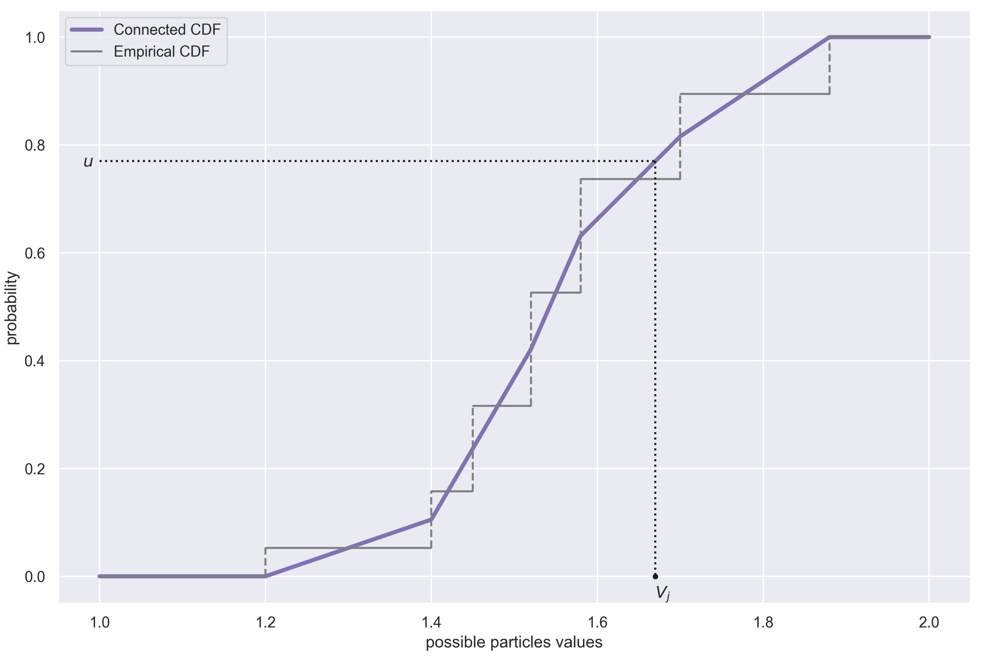
We now want to sample from the probability distribution described by U j to obtain the true “refined” particles. Most sources suggest drawing from it, treating it as a multinomial distribution. However, this makes all the “refined” particles have the same values as the “raw” ones, with just the proportions changed (the same “raw” particle can be drawn several times, if it has a higher probability than the others). To address this problem, we conduct the sampling in a different way. We first need to sort the values of particles in ascending order. Mathematically speaking, we create another sequence and call it V ˜ j s o r t , ensuring that the following conditions are all met:
  • The particle with the smallest value is the first in the new sequence, i.e.,
    V ˜ 1 s o r t ( k Δ t ) = min j { 1 , 2 , , N } { V ˜ j ( k Δ t ) } ,
  • The particle with the largest value is the last in the new sequence, i.e.,
    V ˜ N s o r t ( k Δ t ) = max j { 1 , 2 , , N } { V ˜ j ( k Δ t ) } ,
  • For any j { 2 , 3 , N 1 } , we have
    V ˜ j 1 s o r t ( k Δ t ) < V ˜ j s o r t ( k Δ t ) < V ˜ j + 1 s o r t ( k Δ t ) .
We also want to keep track of the probabilities of our sorted particles; so, we order the probabilities in the same way, by defining another probability sequence W ˘ j s o r t ,
W ˘ j s o r t ( k Δ t ) = W ˘ m ( k Δ t ) for m , such that V ˜ j s o r t ( k Δ t ) U m ( k Δ t ) .
This step is necessary to ensure that each element of the sorted sequence of particle values V ˜ j s o r t still has an original normalised probability W ˘ j s o r t assigned to it. This is why it was necessary to pair up the particles and their normalised probabilities into two-element vectors, under Equation (67). These pairs now help us approximate a continuous distribution, from which we can sample the refined particles. The “extreme” particles, V ˜ 1 s o r t and V ˜ N s o r t , will become the edges of the support of this new continuous distribution. The CDF function is given by the formula below (the time labels have been dropped for the sake of legibility, as all the variables are evaluated at t = k Δ t ):
F V ˜ s o r t ( v ) = 0 if v V ˜ 1 s o r t v V ˜ 1 s o r t V ˜ 2 s o r t V ˜ 1 s o r t ( W ˘ 1 s o r t + 1 2 W ˘ 2 s o r t ) if v ( V ˜ 1 s o r t , V ˜ 2 s o r t ] m = 1 j 1 W ˘ m s o r t + 1 2 W ˘ j s o r t + v V ˜ j s o r t V ˜ j + 1 s o r t V ˜ j s o r t 1 2 W ˘ j s o r t + 1 2 W ˘ j + 1 s o r t if v ( V ˜ j s o r t , V ˜ j + 1 s o r t ] for j { 2 , 3 , N 2 } m = 1 N 2 W ˘ m s o r t + 1 2 W ˘ N 1 s o r t + v V ˜ N 1 s o r t V ˜ N s o r t V ˜ N 1 s o r t 1 2 W ˘ N 1 s o r t + W ˘ N s o r t if v ( V ˜ N 1 s o r t , V ˜ N s o r t ] 1 if v ( V ˜ N s o r t .
The formula might seem overwhelming, but there is a very easy-to-follow interpretation behind it (see Figure 1). The new “refined” particles can be generated by drawing from the distribution given by F V ˜ s o r t ; the simplest way to do so is to use the inverse transform sampling.
V j ( k Δ t ) F V ˜ s o r t .
After following the described procedure for each k { 1 , 2 , , n 1 } , we can specify the actual estimate of the volatility process as the mean of the “refined” particles.
v ( k Δ t ) = 1 N j = 1 N V j ( k Δ t ) .
For k = n , we can simply assume v ( n Δ t ) = v ( n 1 ) Δ t , which should not have any tangible negative impact on any procedure using the v ( t ) estimate for a sufficiently dense time discretisation grid.

3.2. Heston Model with Jumps

The above estimation framework can be used with minor changes to also estimate the Heston model with jumps. The model’s SDE is defined in Equation (6). After the incorporation of jumps, changes are needed particularly in the particle filtering part of the estimation procedure. The particles need to be created not only for various possible values of volatility V j ( t ) but also for the possibility of a jump at that particular moment in time, J j ( t ) , and the size of that jump, Z j ( t ) . So, one can think of a particle as of a three-element “tuple” ( V j , J j , Z j ) . Generating “raw” values for J j and Z j is easy; for each j { 0 , 1 , , N } , J j is simply a random variable from a Bernoulli distribution with parameter λ t h ,
J ˜ j ( k Δ t ) B ( λ t h ) .
Parameter λ t h [ 0 , 1 ) can be thought of as a “threshold” value—a proportion of the number of particles that encodes the occurrence of a jump to all the particles. If the number of jumps is expected to be significant, it is good to increase the value of λ t h , hence increasing the number of particles suggesting the jump in each step. The values of λ t h , which we observe to work reasonably well for most datasets, are between 0.1 and 0.35 . There is a multitude of ways in which one can assess a rational value of this parameter, and one of the most basic ones is visualising the returns of the asset in question and assessing the number of distinct downward spikes on the plot. The ratio of this number and the length of the sample should be a good indication of the region of the interval [ 0.1 , 0.35 ] from which λ t h should be taken.
The raw particles for Z j are simply independent normal random variables with mean μ 0 J and standard deviation σ 0 J , which depict our “prior” beliefs about the size and variance of the jumps
Z ˜ j ( k Δ t ) N ( μ 0 J , σ 0 J ) .
Assigning probabilities to the particles is different as well, since the normal PDF function that we use is different when there is a jump. Hence, Equation (65) needs to be updated to
W ˜ j ( k Δ t ) = 1 2 π V ˜ j ( k 1 ) Δ t Δ t × exp 1 2 R ( k Δ t ) μ i Δ t 1 2 V ˜ j ( k 1 ) Δ t Δ t if J ˜ j = 0 1 exp Z ˜ j ( k Δ t ) 2 π V ˜ j ( k 1 ) Δ t Δ t × exp 1 2 R ( k Δ t ) exp Z ˜ j ( k Δ t ) ( μ i Δ t + 1 ) 2 exp 2 Z ˜ j ( k Δ t ) V ˜ j ( k 1 ) Δ t Δ t if J ˜ j = 1 .
We then normalise W ˜ j so that it sums to 1 and resample V ˜ j , as in the case with no jumps; additionally, we resample Z ˜ j in the exact same way as V ˜ j , i.e., we sort the particles and draw from the distribution F Z ˜ s o r t to obtain the “refined” particles Z j ,
Z j ( k Δ t ) F Z ˜ s o r t .
Finally, for the estimate of λ , for each k { 1 , 2 , n } , one needs to sum the cumulative value of all particles declaring a jump. That way, we obtain a probability that a jump took place at the time t = k Δ t ,
λ ( k Δ t ) = j = 1 N J j ( k Δ t ) W ˘ j ( k Δ t ) .
To obtain the actual estimate of λ , one needs to average λ ( t ) across all the time points obtained for different values of k,
λ i = 1 T k = 1 n λ ( k Δ t ) .
Similarly, to obtain the estimate of μ J and σ J , for each k, one needs to first calculate the average size of a jump from the refined particles,
Z ( k Δ t ) = 1 N j = 1 N Z j ( k Δ t ) ,
and then calculate the mean and standard deviation of the results, weighed by the probability of a jump at time moment t indicated by λ ( t ) . For the weighted mean of the jumps, we obtain
μ i J = k = 1 n Z ( k Δ t ) λ ( k Δ t ) k = 1 n λ ( k Δ t ) 1 ,
and for the standard deviation, we obtain
σ i J = k = 1 n λ ( k Δ t ) Z ( k Δ t ) μ i J 2 n 1 n k = 1 n λ ( k Δ t ) 1 .
The presence of jumps also influences the estimation of other parameters; some of the procedures presented in the previous subsection are not equally applicable, as jumps added to the stock price will additionally increase or more likely decrease the returns. To improve that, a correction of the definitions of R ( t ) is needed in order to “neutralise” the impact of the jumps on the parameters. In other words, Equation (12) should be replaced with
R ( k Δ t ) = S ( k Δ t ) S ( k 1 ) Δ t ) 1 λ ( k Δ t ) 1 exp Z ( k Δ t ) .
Note that the added term has a value very close to 1 when λ ( t ) is close to 0, which indicates there was no jump at time t; so, the correction to the “original” value of R ( t ) is very minor. However, if λ ( t ) is close to 1, which means there was a jump, the value of the term becomes close to exp Z ( t ) , which is an inverse of the jump factor (with the estimated jump size Z ( t ) ). Multiplying by that inverse brings the value of R ( t ) to a level as if there was no jump at time t (see Figure 2), and the estimation of the parameters of the model can be carried out as before.

3.3. Estimation Procedure

The Bayesian estimation framework presented above relies on several parameters for the prior distributions that cannot be calculated within the procedure itself. They are often referred to as metaparameters. For example, for the estimation of the μ parameter, the values of two metaparameters are required, μ 0 η and τ 0 η (see Equations (19) and (20)). Their values should reflect our preexisting beliefs regarding the value of the parameter that we are trying to estimate, μ in this case. Let us say that for a given trajectory of the Heston model process, we assume the value of μ to be around 0.5 . What values should we then choose for the metaparameters? First of all, we need to note that μ 0 η and τ 0 η are not the parameters of the prior distribution for μ directly. They are parameters of another random variable, which we introduced to utilise the Bayesian framework, namely η . The connection between μ and η is known and given by Equation (11). Hence, if we assume μ to be around a certain value, then using this relationship, we can deduce the value of η . In addition, since the prior distibution of η is normal, with the mean μ 0 η and the variance σ 0 η = 1 τ 0 η , we can propose the value of the mean of this distribution to be whatever η is for the supposed value of μ . Selecting a value for σ 0 η (and thus τ 0 η ) is even more equivocal; it should reflect the level of confidence that we have for choosing a mean parameter. That is, if we feel that the value we chose for μ 0 η would bring us close to the true μ , we should choose a smaller value for σ 0 η . However, if we are not as sure about it, a larger value of σ 0 η should be used. A similar analysis can be repeated for choosing the values of the other metaparameters. We need to be aware that the prior used always in some way influences the final estimate of a given parameter. More detailed analysis on this topic is given in Section 4.2.
Another problem that emerges when applying Bayesian inference (especially for more complex models) is that estimating one parameter often requires knowing the value of some of the others and vice versa. Hence, there is not an obvious way of how to start the whole procedure. One way to address this problem is to provide the initial guesses for the values of all the parameters (as described in the paragraph above) and use them in the first round of samplings. A well-designed MCMC estimation algorithm should bring us closer to the true values of parameters with each new round of samplings. In Algorithms 1 and 2, our procedure for the Heston model without and with jumps is shown, respectively. The meaning of all symbols is briefly summarised in Appendix A.
Algorithm 1:Estimating the Heston model
Require:
  • number of samples: n s
  • time step Δ t
  • maturity T
  • prices S ( k Δ t ) for k { 0 , 1 , , n } , so that n Δ t = T
  • number of particles N
  • initial value of μ : μ 0
  • initial value of κ : κ 0
  • initial value of θ : θ 0
  • initial value of σ : σ 0
  • initial value of ρ : ρ 0
  • prior distribution parameters for η : μ 0 η and τ 0 η
  • prior distribution parameters for β : μ 0 β and Λ 0 β
  • prior distribution parameters for σ 2 : a 0 σ and b 0 σ
  • prior distribution parameters for ψ : μ 0 ψ and τ 0 ψ
  • prior distribution parameters for ω : a 0 ω and b 0 ω
Ensure:
  • estimate of parameter μ : μ ^
  • estimate of parameter κ : κ ^
  • estimate of parameter θ : θ ^
  • estimate of parameter σ : σ ^
  • estimate of parameter ρ : ρ ^
  • estimate of the volatility process: v ( t )
  • for  k = 1 n  do
  •     set R ( k Δ t ) , as shown in Equation (12)
  • end for
  • for  i = 0 n s  do
  •     for  k = 1 n 1  do             ▹ particle filtering procedure
  •         for  j = 1 N  do
  •            obtain V j ( k Δ t ) , as shown in Equations (60)–(73)
  •         end for
  •         obtain v ( k Δ t ) , as shown in Equation (74)
  •     end for
  •     obtain μ i , as shown in Equations (13)–(23)
  •     obtain κ i , θ i , and σ i , as shown in Equations (25)–(44)
  •     obtain ρ i , as shown in Equations (45)–(59)
  • end for
  • set μ ^ = 1 n s i = 1 n s μ i
  • set κ ^ = 1 n s i = 1 n s κ i
  • set θ ^ = 1 n s i = 1 n s θ i
  • set σ ^ = 1 n s i = 1 n s σ i
  • set ρ ^ = 1 n s i = 1 n s ρ i
Algorithm 2:Estimating the Heston model with jumps
Require:
  • number of samples: n s
  • time step Δ t
  • maturity T
  • prices S ( k Δ t ) for k { 0 , 1 , , n } , so that n Δ t = T
  • number of particles N
  • initial value of μ : μ 0
  • initial value of κ : κ 0
  • initial value of θ : θ 0
  • initial value of σ : σ 0
  • initial value of ρ : ρ 0
  • prior distribution parameters for η : μ 0 η and τ 0 η
  • prior distribution parameters for β : μ 0 β and Λ 0 β
  • prior distribution parameters for σ 2 : a 0 σ and b 0 σ
  • prior distribution parameters for ψ : μ 0 ψ and τ 0 ψ
  • prior distribution parameters for ω : a 0 ω and b 0 ω
  • ratio of particle indicating jumps: λ t h
  • prior distribution parameters for Z: μ 0 J and σ 0 J
Ensure:
  • estimate of parameter μ : μ ^
  • estimate of parameter κ : κ ^
  • estimate of parameter θ : θ ^
  • estimate of parameter σ : σ ^
  • estimate of parameter ρ : ρ ^
  • estimate of the volatility process: v ( t )
  • for  k = 1 n  do
  •     set R ( k Δ t ) , as shown in Equation (12)
  • end for
  • for  i = 0 n s  do
  •     for  k = 1 n  do             ▹ particle filtering procedure
  •         for  j = 1 N  do
  •            generate J ˜ j ( k Δ t ) , as shown in Equation (75)
  •            generate Z ˜ j ( k Δ t ) , as shown in Equation (76)
  •            obtain V j ( k 1 ) Δ t , as shown in Equations (61)–(73) and (77)
  •         end for
  •         obtain v ( k Δ t ) , as shown in Equation (74)
  •         obtain Z ( k Δ t ) and λ ( k Δ t ) , as shown in Equations (78)–(79) and (81)
  •     end for
  •     for  k = 1 n  do
  •         update R ( k Δ t ) , as shown in Equation (84)
  •     end for
  •     obtain μ i , as shown in Equations (13)–(23)
  •     obtain κ i , θ i , and σ i as shown in Equations (25)–(44)
  •     obtain ρ i , as shown in Equations (45)–(59)
  •     obtain λ i , as shown in Equation (80)
  •     obtain μ i J , as shown in Equation (82)
  •     obtain σ i J , as shown in Equation (83)
  • end for
  • set μ ^ = 1 n s i = 1 n s μ i
  • set κ ^ = 1 n s i = 1 n s κ i
  • set θ ^ = 1 n s i = 1 n s θ i
  • set σ ^ = 1 n s i = 1 n s σ i
  • set ρ ^ = 1 n s i = 1 n s ρ i
  • set λ ^ = 1 n s i = 1 n s λ i
  • set μ J ^ = 1 n s i = 1 n s μ i J
  • set σ J ^ = 1 n s i = 1 n s σ i J

4. Analysis of the Estimation Results

4.1. Exemplary Estimation

We present here an exemplary estimation of the Heston model with jumps, to show the outcomes of the entire procedure. We assumed relatively noninformative prior distributions, with expected values shifted from the true parameters to make the task more challenging for the algorithm and to better reflect the real-life situation in which the priors used do not match the true parameters exactly most of the time, but they should be rather close to them. Table 1 lists all the values of the priors we used. Table 2 summarises the results obtained, and Figure 3 elaborates on those results by showing the empirical distributions of the samples for all parameters of the model.
Analysing the sample estimates for each of the parameters (presented in Figure 3), one can observe that for most of them (Figure 3a–e,h), the true value of the parameter was within the support of the distribution of all samples. However, in case of two parameters, λ and μ J (Figure 3f and Figure 3g, respectively), the scope of the samples generated by the estimation procedure seemed not even to include the parameter’s true value. This was due to the fact that those parameters were related to the intensity and size of the jumps, and for the simulation parameters we chose, those jumps did not occur frequently (as in case of real-life price falls). Hence, even though the procedure correctly identified the moments of the jumps and estimated their sizes, those estimates were relatively far from the true values, simply because there was very little source material for the estimation in the first place. To be precise, the stock price simulated for our exemplary estimation experienced four jumps, and the times of those jumps were easily identified by our procedure with almost 100% certainty. Thus, since the length of time of the price observation (in years) was T = 3 , the most probable value of the jump intensity λ was around 4 3 (compared to the actual result in Table 2), although, obviously, the other values of λ (slightly smaller or larger) could also have led to four jumps, and this was exactly what happened in our case, as our true intensity was λ = 1 (again, see Table 2). Similarly, in the case of μ J , the reason for the estimated average jump to be larger (in terms of magnitude) than the actual one was that the four jumps, which were simulated, all happened to be more severe than the true value of μ J would suggest (by pure chance), and this “pushed” the procedure towards overestimating the (absolute) size of the jump.

4.2. Important Findings

Although estimation through the joint forces of Bayesian inference, Monte Carlo Markov chains, and particle filtering is generally considered very effective Johannes and Polson (2010), it has several areas the user needs to be aware of while using this estimation scheme. One of the issues worth considering is the impact of the prior parameters. A Bayesian estimator of any kind needs to be fed with the parameters of the prior distribution, which should reflect our preexisting beliefs of what the value of the actual estimated parameter could be. The amount of information conveyed by a prior can be different, depending on several factors. One of these is the parameters of the prior distribution itself. Consider μ 0 η and σ 0 η , mentioned already in the previous section. They are the prior parameters for η , the predecessor for the μ estimates. The larger the σ 0 η we take, the more volatile the estimates of η and μ are going to be. This is a pretty intuitive fact, being a direct consequence of the Bayesian approach itself. A more subtle influence of priors is hidden in the alternation between the MCMC sampling and particle filtering procedures.
As mentioned in the previous section, the MCMC and particle filtering depend on one another. As can be seen in Algorithms 1 and 2, we took the approach that the particle filtering procedure should be conducted first, and the singular parameters that it needed should be the expected values of the prior distributions that we assumed. Having the volatility estimated this way, we can estimate the parameters and, based on them, re-estimate the volatility process, and so on. Although we can keep alternating that way as many times as we want, until the planned end of the estimation procedure, one might be tempted to perform the particle filtering procedure fewer times, as it is much more computationally expensive than the MCMC draws. The premise for this would be that after several trials, the volatility estimate becomes “good enough”, and from that point onward, one could solely generate more MCMC samples. A critical observation that we have made is that the quality of the initial volatility estimates depends very highly on the prior parameters that were used to initiate it. With a small number of particle filtering procedures followed by multiple MCMC draws, the entire scheme does not have “enough time” to properly calibrate, and the results tend to stick to the priors that are used. That means for a prior leading exactly to the true value of the parameter, the estimator returns almost error-free results; however, if one uses a prior leading to value of the true parameter, e.g., 20% larger than it really is, the estimate will probably be off by roughly 20%, which does not make the estimator very useful. A counterproposal can then be made to perform particle filtering as long as possible. This, however, is not an ideal solution either. Firstly, as we said, it is very computationally expensive, and secondly, a very long chain of samples increases the probability that the estimation procedure would at some point return an “outlier”, i.e., an estimate far away from the true value of the parameter, which is especially likely if we use metaparameters responsible for such a parameter’s larger variance (e.g., σ 0 η for η ). The appearance of such “outliers” is especially unfavourable in case of the MCMC methods, since its nature is that each sample is directly dependent on the previous one; so, the whole procedure is likely to “stay” in the given “region” of the parameter space for some number of subsequent simulations, thus impacting the final estimate of the parameter (which is the mean of all the observed samples). Therefore, a clear tradeoff appears. If we believe strongly that the prior we use is rather correct and only needs some “tweaking” to adjust it to the particular dataset, a modest amount of particle filtering can be applied2, followed by an arbitrary number of MCMC draws. If, however, we do not know much about our dataset and do not want to convey too much information through the prior, even at the cost of slightly worse final results, we should run particle filtering for a larger number of times. The visual interpretation of this rule is presented in Figure 4 and Figure 5.
Another factor which should be taken into consideration using the Bayesian approach for estimating the Heston model is that the quality of results depends highly on the very parameters we try to estimate. The σ parameter seems to play a critical role for the Heston model, in particular. This can be observed in Figure 6. To produce it, an identical estimation procedure was performed for two sample paths (which we can think of as of two different stocks). They were simulated with the same parameters, except for σ . Path no. 1 was simulated with σ = 0.01 and path no. 2 with σ = 0.1 , ten times larger. The histograms present the distribution of the estimated values of the κ parameter; the true κ was κ = 1 , and the red vertical line illustrates this true value. It is clearly visible that for the value of σ = 0.01 , the samples were much more concentrated around the true value, while for a larger value of σ = 0.1 , they were more dispersed, and the variance of the distribution was significantly larger. This incommodity cannot be easily resolved, as the true values of the parameters of the trajectories are idiosyncratic; they cannot be influenced by the estimation procedure itself. However, we wanted to sensitise the reader to the fact that the larger the value of σ , the less trustworthy the results of the estimation of the other parameters might be.

4.3. Towards Real-Life Applications

At the end, we wanted to emphasise the applicability of the methods described above to real market data. We briefly mentioned in the Introduction that the results yielded by some investment strategies are dependent on the character of the asset, which might be accurately captured by parameters of the models we used to model this asset (see Gruszka and Szwabiński (2021) for more details). Having a tool for obtaining the values of those parameters from the data opens up a new field of investigation relying on comparing synthetically generated stock price trajectories to the real ones and selecting optimal portfolio management strategies based on the results of such comparisons. We explore the possibility of utilising parameter estimates this exact way in our other work; see Gruszka and Szwabiński (2023).

5. Conclusions

In this paper, a complete estimation procedure of the Heston model without and with jumps in the asset prices was presented. Bayesian regression combined with the particle filtering method was used as the estimation framework. Although some parts of the procedure have been used in the past, our work provides the first complete follow-along recipe of how to estimate the Heston model for real stock market data. Moreover, we presented a novel approach to handle jumps in order to neutralize their negative impact on the estimates of the key parameters of the model. In addition, we proposed an improvement of the sampling in the particle filtering method to obtain a better estimate of the volatility.
We extensively analysed the impact of the prior parameters as well as the number of MCMC samplings and particle filtering iterations on the performance of our procedure. Our findings may help to avoid several difficulties related with the Bayesian methods and apply them successfully to the estimation of the model.
Our results have an important practical impact. In one of our recent papers, Gruszka and Szwabiński (2021), we showed that the relative performance of several investment strategies within the Heston model varied with the values of its parameters. In other words, what turned out to be the best strategy in one range of the parameter values may have been the worst one in the others. Thus, determining which parameter of the model corresponds to a given stock market will allow one to choose the optimal investment strategy for that market.

Author Contributions

Conceptualization, J.G. and J.S.; methodology, J.G.; software, J.G.; validation, J.S.; formal analysis, J.S.; investigation, J.G.; resources, J.G.; data curation, J.G.; writing—original draft preparation, J.G.; writing—review and editing, J.S.; visualization, J.G.; supervision, J.S.; project administration, J.S. All authors have read and agreed to the published version of the manuscript.

Funding

This research received no external funding.

Data Availability Statement

All the data used throughout the article was synthetically simulated using models and methods outlined in the content of the article, no real-life data was used. Authors will respond to the individual requests for sharing the exact data sets simulated for the purpose of this article raised via e-mail to the corresponding author.

Conflicts of Interest

The authors declare no conflict of interest.

Appendix A. Table of Symbols

Table A1. Table of symbols used throughout the article.
QuantityExplanation
Tmax time (i.e., t [ 0 , T ] )
S ( t ) asset price (with S ( 0 ) S 0 )
v ( t ) volatility (with v ( 0 ) v 0 )
B S ( t ) Brownian motion for the price process
B v ( t ) Brownian motion for the volatility process
μ drift
κ rate of return to the long-time average
θ long-time average
σ volatility of the volatility
ρ correlation between prices and volatility
Z ( t ) size of the jump
μ J mean of the jump size
σ J standard deviation of the jump size
q ( t ) Poisson process counting jumps
λ intensity of jumps
Δ t time step (also known as the discretisation constant)
nnumber of time steps (also known as the length of data)
ε S ( t ) price process random component
ε v ( t ) volatility process random component
ε a d d ( t ) additional random component—see Equation (10))
η regression parameter for drift estimation—see Equation (11)
R ( t ) ratio between neighbouring prices—see Equations (12) and (84)
y S ( t ) series of dependent variables for the drift estimation—see Equation (14)
x S ( t ) series of independent variables for the drift estimation—see Equation (15)
y S vector of the dependent variable for the drift estimation—see Equation (17)
x S vector of the independent variable for the drift estimation—see Equation (18)
μ 0 η mean of the prior distribution of η
σ 0 η standard deviation of the prior distribution of η
Table A2. Table of symbols used throughout the article (continued).
QuantityExplanation
τ 0 η precision of the prior distribution of η
η ^ OLS estimator of η —see (21)
μ η mean of the posterior distribution of η —see (20)
τ η precision of the posterior distribution of η —see (19)
η i i-th sample of η —see (22)
μ i i-th estimate of the drift—see (23)
β 1 regression parameter for volatility parameters estimation—see Equation (25)
β 2 regression parameter for volatility parameters estimation—see Equation (26)
β vector of regression parameters for volatility parameters estimation—see Equation (29)
y v vector of the dependent variable for the volatility parameter estimation—see Equation (30)
x 1 v vector of the independent variable for the volatility parameter estimation—see Equation (31)
x 2 v vector of the independent variable for the volatility parameter estimation—see Equation (32)
X v matrix of the independent variable for the volatility parameter estimation—see Equation (34)
ε v noise vector of the volatility parameter estimation—see Equation (35)
μ 0 β mean vector of the prior distribution of β
Λ 0 β precision matrix of the prior distribution of β
μ β mean vector of the posterior distribution of β —see Equation (37)
Λ β precision matrix of the posterior distribution of β —see (36)
β ^ OLS estimator of β —see (38)
β i i-th sample of β —see (39)
κ i i-th estimate of κ —see (40)
θ i i-th estimate of θ —see (41)
a 0 σ shape parameter of the prior distribution of σ 2
b 0 σ scale parameter of the prior distribution of σ 2
a σ shape parameter of the posterior distribution of σ 2
b σ scale parameter of the posterior distribution of σ 2
σ i i-th estimate of the σ —see (42)
e 1 ρ ( t ) series of residuals of the price equation—see (45)
e 2 ρ ( t ) series of residuals of the volatility equation—see (46)
ψ regression parameter for ρ estimation, ψ = σ ρ —see (47)
ω regression parameter for ρ estimation, ω = σ 2 ( 1 ρ 2 ) —see (47)
e 1 ρ ( t ) series of independent variables for the estimation of ρ —see (45)
e 2 ρ ( t ) series of dependent variables for the estimation of ρ —see (46)
e 1 ρ vector of the independent variables for the estimation of ρ —see (50)
e 2 ρ vector of the dependent variables for the estimation of ρ —see (51)
e ρ matrix of residuals—see (52)
A ρ auxiliary matrix for solving ρ regression—see (53)
μ 0 ψ mean of the prior distribution of ψ
τ 0 ψ precision of the prior distribution of ψ
μ ψ mean of the posterior distribution of ψ —see (54)
τ ψ precision of the posterior distribution of ψ —see (55)
a 0 ω shape parameter of the prior distribution of ω
b 0 ω scale parameter of the prior distribution of ω
a ω shape parameter of the posterior distribution of ω —see (56)
b ω scale parameter of the posterior distribution of ω —see (57)
ψ i i-th sample of ψ —see (59)
ω i i-th sample of ω —see (58)
ε j ( t ) j-th sample of particle filtering independent errors—see (61)
z j ( t ) j-th sample of particle filtering residuals—see (62)
w j ( t ) j-th sample of particle filtering correlated—see (62)
V ˜ j ( t ) j-th raw volatility particle—see (64)
W ˜ j ( t ) j-th particle likelihood measure—see (65) and (77)
W ˘ j ( t ) j-th particle probability—see (66)
U j ( t ) j-th particle-probability vector—see (67)
V ˜ j s o r t ( t ) j-th raw volatility particle in a sorted sequence—see (68), (69), and (70)
W ˘ j s o r t ( t ) probability of the j-th particle in the sorted sequence—see (71)
F V ˜ s o r t ( v ) continuous CDF of resampled particles—see (72)
Table A3. Table of symbols used throughout the article (continued).
QuantityExplanation
V j ( t ) j-th final volatility particle—see (73)
λ t h proportion of particles encoding a jump
J ˜ j ( t ) j-th raw moment-of-a-jump particle—see (75)
μ 0 J mean of the raw size-of-a-jump particle
σ 0 J standard deviation of the raw size-of-a-jump particle
Z ˜ j ( t ) j-th raw size-of-a-jump particle—see (76)
Z j ( t ) j-th resampled size-of-a-jump particle—see (78)
λ ( t ) probability of a jump—see (79)
λ i i-th estimate of λ —see (80)
Z ( t ) estimate of an average size of a jump—see (81)
μ i J i-th estimate of μ J —see (82)
σ i J i-th estimate of σ J —see (83)

Notes

1
Equation (65) is the reason we cannot run this procedure for k = n , as we would not be able to obtain R ( n + 1 ) Δ t , since the last available value is R ( n Δ t ) .
2
For applications in finance, this task is sometimes easier than for some other fields of science, as numerous works have been published already, presenting the results of the estimates of well-known stocks or market indices within various models. See, e.g., Eraker et al. (2003)

References

  1. Bates, David S. 1996. Jumps and Stochastic Volatility: Exchange Rate Processes Implicit in Deutsche Mark Options. The Review of Financial Studies 9: 69–107. [Google Scholar] [CrossRef]
  2. Black, Fischer, and Myron Scholes. 1973. The Pricing of Options and Corporate Liabilities. Journal of Political Economy 81: 637–54. [Google Scholar] [CrossRef] [Green Version]
  3. Chib, Siddhartha, and Edward Greenberg. 1995. Understanding the Metropolis-Hastings Algorithm. The American Statistician 49: 327–35. [Google Scholar] [CrossRef] [Green Version]
  4. Christoffersen, Peter, Kris Jacobs, and Karim Mimouni. 2007. Volatility Dynamics for the S&P500: Evidence from Realized Volatility, Daily Returns and Option Prices. Rochester: Social Science Research Network. [Google Scholar] [CrossRef]
  5. Cox, John C., Jonathan E. Ingersoll, and Stephen A. Ross. 1985. A Theory of the Term Structure of Interest Rates. Econometrica 53: 385–407. [Google Scholar] [CrossRef]
  6. Doucet, Arnaud, and Adam Johansen. 2009. A Tutorial on Particle Filtering and Smoothing: Fifteen Years Later. Handbook of Nonlinear Filtering 12: 3. [Google Scholar]
  7. Eraker, Bjørn, Michael Johannes, and Nicholas Polson. 2003. The Impact of Jumps in Volatility and Returns. The Journal of Finance 58: 1269–300. [Google Scholar] [CrossRef]
  8. Gruszka, Jarosław, and Janusz Szwabiński. 2021. Advanced strategies of portfolio management in the Heston market model. Physica A: Statistical Mechanics and Its Applications 574: 125978. [Google Scholar] [CrossRef]
  9. Gruszka, Jarosław, and Janusz Szwabiński. 2023. Portfolio optimisation via the heston model calibrated to real asset data. arXiv arXiv:2302.01816. [Google Scholar]
  10. Heston, Steven. 1993. A Closed-Form Solution for Options with Stochastic Volatility with Applications to Bond and Currency Options. The Review of Financial Studies 6: 327–43. [Google Scholar] [CrossRef] [Green Version]
  11. Jacquier, Eric, Nicholas G. Polson, and Peter E. Rossi. 2004. Bayesian analysis of stochastic volatility models with fat-tails and correlated errors. Journal of Econometrics 122: 185–212. [Google Scholar] [CrossRef]
  12. Johannes, Michael, and Nicholas Polson. 2010. CHAPTER 13—MCMC Methods for Continuous-Time Financial Econometrics. In Handbook of Financial Econometrics: Applications. Edited by Yacine Aït-Sahalia and Lars Peter Hansen. San Diego: Elsevier, vol. 2, pp. 1–72. [Google Scholar] [CrossRef]
  13. Johannes, Michael, Nicholas Polson, and Jonathan Stroud. 2009. Optimal Filtering of Jump Diffusions: Extracting Latent States from Asset Prices. Review of Financial Studies 22: 2559–99. [Google Scholar] [CrossRef]
  14. Kloeden, Peter, and Eckhard Platen. 1992. Numerical Solution of Stochastic Differential Equations, 1st ed. Stochastic Modelling and Applied Probability. Berlin/Heidelberg: Springer. [Google Scholar]
  15. Lindley, Dennis. V., and Adrian F. M. Smith. 1972. Bayes Estimates for the Linear Model. Journal of the Royal Statistical Society: Series B (Methodological) 34: 1–18. [Google Scholar] [CrossRef]
  16. Meissner, Gunter, and Noriko Kawano. 2001. Capturing the volatility smile of options on high-tech stocks—A combined GARCH-neural network approach. Journal of Economics and Finance 25: 276–92. [Google Scholar] [CrossRef]
  17. O’Hagan, Anthony, and Maurice George Kendall. 1994. Kendall’s Advanced Theory of Statistics: Bayesian Inference. Volume 2B. London: Arnold. [Google Scholar]
  18. Wong, Bernard, and Chris C. Heyde. 2006. On changes of measure in stochastic volatility models. International Journal of Stochastic Analysis 2006: 018130. [Google Scholar] [CrossRef]
Figure 1. Visualisation of the process of resampling particles according to their probabilities. The values of the raw particles are the places, where the empirical cumulative distribution function (ECDF in short) jumps, and each jump size represents the probability of a respective raw particle. The connected CDF is a continuous modification of the ECDF, built according to Formula (72). In order to resample, a uniform random variable u is generated, and then its inverse through the connected CDF function becomes a new resampled particle, V j .
Econometrics 11 00015 g001
Figure 2. Comparison of the returns for a process with jumps calculated based on Formula (12) (blue line) and (84) (orange line). It can be clearly seen that the jumps have been “neutralised” in the latter case.
Econometrics 11 00015 g002
Figure 3. Empirical PDFs of the exemplary Heston parameter estimates. (a) parameter μ . (b) parameter κ . (c) parameter θ . (d) parameter σ . (e) parameter ρ . (f) parameter λ . (g) parameter μ J . (h) parameter σ J .
Econometrics 11 00015 g003
Figure 4. Empirical distributions of the estimate samples for the θ parameter in the case when the mean of the prior distribution exactly matches the true parameter and when it is twice as large. The distributions in (a) were based on 10 sampling cycles and in (b) on 500 cycles. One can observe that for the first figure, the distribution with the exact prior gives very good results, much better than the shifted one. In the second figure, both distributions are comparable.
Econometrics 11 00015 g004
Figure 5. Sequences of estimate samples for a procedure in which particle filtering was conducted only for the first 5% of samplings and another one in which the particle filtering was conducted for all the samplings. In both cases, the mean of the prior distribution was shifted by 100% compared to its true value. It can be observed that the samples of the first procedure remained around the value close to the one dictated by the prior, whereas the samples of the other procedure converged to the true value of the parameter, which led to the better final result, less dependent on the prior parameters.
Econometrics 11 00015 g005
Figure 6. Empirical distributions of the estimate samples for the κ parameter of two different trajectories of the Heston model—one with σ = 0.01 and the other with σ = 0.1 . The distribution of the estimate samples of the trajectory with a smaller value of σ is narrower and more concentrated; hence, it is likely to give less variable final estimates.
Econometrics 11 00015 g006
Table 1. Priors for the exemplary estimation procedure.
Prior ParameterValue
μ 0 η 1.00125
σ 0 η 0.001
Λ 0 10 0 0 5
μ 0 35 × 10 6 0.988
a 0 σ 149
b 0 σ 0.025
μ 0 ψ 0.45
σ 0 ψ 0.3
a 0 ω 1.03
b 0 ω 0.05
λ t h 0.15
μ 0 J 0.96
σ 0 J 0.3
Table 2. Results of the exemplary estimation procedure.
ParameterTrue ValueEstimated ValueRelative Error [%]
μ 0.10.098291.77
κ 11.219021.90
θ 0.050.04931.92
σ 0.010.01088.55
ρ −0.50.437912.40
λ 11.334933.49
μ J −0.8−0.965120.64
σ J 0.20.229814.88
Disclaimer/Publisher’s Note: The statements, opinions and data contained in all publications are solely those of the individual author(s) and contributor(s) and not of MDPI and/or the editor(s). MDPI and/or the editor(s) disclaim responsibility for any injury to people or property resulting from any ideas, methods, instructions or products referred to in the content.

