Nonfractional Long-Range Dependence: Long Memory, Antipersistence, and Aggregation

Abstract

This paper used cross-sectional aggregation as the inspiration for a model with long-range dependence that arises in actual data. One of the advantages of our model is that it is less brittle than fractionally integrated processes. In particular, we showed that the antipersistent phenomenon is not present for the cross-sectionally aggregated process. We proved that this has implications for estimators of long-range dependence in the frequency domain, which will be misspecified for nonfractional long-range-dependent processes with negative degrees of persistence. As an application, we showed how we can approximate a fractionally differenced process using theoretically-motivated cross-sectional aggregated long-range-dependent processes. An example with temperature data showed that our framework provides a better fit to the data than the fractional difference operator.

1. Introduction

Long-range dependence has been a topic of interest in econometrics since Granger’s study on the shape of the spectrum of economic variables (Granger 1966). The author found that long-term fluctuations in economic variables, if decomposed into frequency components, are such that the amplitudes of the components decrease smoothly with decreasing period. As shown by Adenstedt (1974), this type of behavior implies long-lasting autocorrelations, that is they exhibit long-range dependence. In finance, long-range dependence has been estimated in volatility measures, inflation, and energy prices; see, for instance, Baillie et al. (2019), Vera-Valdés (2021b), Hassler and Meller (2014), and Ergemen et al. (2016).

In the time series literature, the fractional difference operator has become one of the most popular methods to model long-range dependence. Notwithstanding its popularity, Granger argued that processes generated by the fractional difference operator fall into the area of “empty boxes”, about theory—either economic or econometric—on topics that do not arise in the actual economy (Granger 1999). Moreover, Veitch et al. (2013) showed that fractionally differenced processes are brittle in the sense that small deviations such as adding small independent noise change the asymptotic variance structure qualitatively.

This paper developed an econometric-based model for long-range dependence to alleviate these concerns. One of the most cited theoretical explanations behind the presence of long-range dependence in real data is cross-sectional aggregation (Granger 1980). We used cross-sectional aggregation as the inspiration for a nonfractional long-range-dependent model that arises in the actual economy.

The proposed model is simple to implement in real applications. In particular, we present two algorithms to generate long-range dependence by cross-sectional aggregation with similar computational requirements as the fractional difference operator. One is based on the linear convolution form of the process, while the second uses the discrete Fourier transform. The proposed algorithms are exact in the sense that no approximation to the number of aggregating units is needed. We showed that the algorithms can be used to reduce computational times for all sample sizes.

Moreover, we proved that cross-sectionally aggregated processes do not possess the antipersistent properties. We argue that these are restrictions imposed by the fractional difference operator that may not hold in real data. In this regard, the proposed model relaxes these restrictions, and it is thus less brittle than fractional differencing.

We showed that relaxing the antipersistent restrictions has implications for semiparametric estimators of long-range dependence in the frequency domain. In particular, we proved that estimators based on the log-periodogram regression are misspecified for long-range-dependent processes generated by cross-sectional aggregation. To solve the misspecification issue, we developed the maximum likelihood estimator for cross-sectionally aggregated processes. We used the recursive nature of the Beta function to speed up the computations. The estimator inherits the statistical properties of the maximum likelihood.

Finally, as an application, this paper illustrated how we can approximate a fractionally differenced process with a theoretically-based cross-sectionally aggregated one. Thus, we demonstrated that we can model similar behavior as the one induced by the fractional difference operator while providing theoretical support. Moreover, we used temperature data to show that the model provides a better, theoretically supported, fit to real data than the fractional difference operator when the source of long-range dependence is cross-sectional aggregation.

This paper proceeds as follows. In Section 2, we present two distinct ways to generate long-range-dependent processes. Section 3 discusses three different ways to generate cross-sectionally aggregated processes, two of them with similar computational requirements as for the fractional difference operator. Section 4 discusses the antipersistence properties. Section 5 develops the maximum likelihood estimator for cross-sectionally aggregated processes. Section 6 shows a way to generate cross-sectionally aggregated processes that closely mimic the ones generated using the fractional difference operator and shows that the model provides a better fit to real data when the source of long-range dependence is cross-sectional aggregation. Section 7 concludes.

2. Long-Range-Dependent Models

This section presents two mechanisms to generate long-range dependence: the fractional difference operator and cross-sectional aggregation.

2.1. The Fractional Difference Operator

References Granger and Joyeux (1980) and Hosking (1981) proposed to use the fractional difference operator to model long-range dependence in the time series literature. It is defined as:

$$x_t={(1-L)}^d{\epsilon }_t,$$

(1)

where ${\epsilon }_t$ is a white noise process with variance ${\sigma }^2$ and $d\in (-1/2,1/2)$. Following the standard binomial expansion, the fractional difference operator, ${(1-L)}^d$, is decomposed to generate a series given by:

$$x_t=\sum _{k=0}^{\infty }{\pi }_k{\epsilon }_{t-k},$$

(2)

with coefficients ${\pi }_k=\mathsf{\Gamma }(k+d)/\left(\mathsf{\Gamma }\left(d\right)\mathsf{\Gamma }(k+1)\right)$ for $k\in \mathbb{N}$, where $\mathsf{\Gamma }\left(\right)$ denotes the Gamma function. We write $x_t\sim I\left(d\right)$ to denote a process generated by the fractional difference operator (1), that is a fractionally integrated process with parameter d.

For $d\in (0,1/2)$, we call $x_t$ a long memory process, while for $d\in (-1/2,0)$, we call $x_t$ an antipersistent process. To avoid confusion, in this paper, we maintained that a series shows long-range dependence if it has hyperbolic decaying autocorrelations, while we reserved the long memory and antipersistent terminology to specific signs of the parameter d; see Haldrup and Vera-Valdés (2017) for a discussion about the different long-range dependence definitions.

Using Stirling’s approximation, it can be shown that the coefficients in (2) decay at a hyperbolic rate, ${\pi }_k\approx k^{d-1}$ as $k\to \infty$, where we used the notation $f\left(k\right)\approx g\left(k\right)$ as $k\to k_0$ to denote that ${lim}_{k\to k_0}f\left(k\right)/g\left(k\right)=1$. In turn, the autocorrelation function for a fractionally integrated process, ${\gamma }_{I\left(d\right)}\left(k\right)$, is given by:

$${\gamma }_{I\left(d\right)}\left(k\right)=\frac{\mathsf{\Gamma }(k+d)\mathsf{\Gamma }(1-d)}{\mathsf{\Gamma }(k-d+1)\mathsf{\Gamma }\left(d\right)}.$$

(3)

Thus, ${\gamma }_{I\left(d\right)}\left(k\right)\approx k^{2d-1}$ as $k\to \infty$, so that $I\left(d\right)$ processes exhibit long-range dependence regardless of the sign of the parameter d.

The properties of the fractional difference operator have been well documented in, among others, Baillie (1996) and Beran et al. (2013). Moreover, fractionally integrated models obtain good forecasting performance when working with series that exhibit long-range dependence regardless of their generating process; see Bhardwaj and Swanson (2006) and Vera-Valdés (2020). Furthermore, fast algorithms have been developed to generate series using the fractional difference operator; see Jensen and Nielsen (2014). Thus, the fractional difference operator has become the canonical construction for long-range dependence modeling in the time series literature.

Even though the fractional difference operator provides a representation of long-range dependence, there are insufficient theoretical arguments linking the fractional difference operator with the long-range dependence found in real data. Chevillon et al. (2018) presented the only argument to date linking fractional integration to economic models. The authors showed that a large-dimensional vector autoregressive model can generate fractional integration in the marginalized univariate series. Nonetheless, the argument requires strong assumptions regarding the form of the system, and it is only capable of generating fractionally integrated processes with positive degrees of long-range dependence, that is antipersistence is omitted in the analysis.

Granger commented on the lack of theoretical support by arguing that fractionally integrated processes fall in the “empty box” category of topics that do not arise in the real economy. In this regard, the next subsection discusses cross-sectional aggregation, the most common theoretical motivation behind long-range dependence in real data.

2.2. Cross-Sectional Aggregation

Robinson (1978) was the first to analyze the statistical properties of autoregressive processes with random coefficients. He considered a series given by:

$$x_{j,t}={\alpha }_j{x}_{j,t-1}+{ϵ}_{j,t}$$

(4)

where ${\epsilon }_{j,t}$ is an independent identically distributed process with $E\left[{ϵ}_{j,t}\right]=0$ and $E\left[{ϵ}_{j,t}^2\right]={\sigma }^2$, $\forall t\in \mathbb{Z}$. Furthermore, ${\alpha }_j^2$ is sampled from the Beta distribution, independent of ${\epsilon }_{j,t}$, with the following density:

$$\mathcal{B}(\alpha ;a,b)=\frac{1}{B(a,b)}{\alpha }^{a-1}{(1-\alpha )}^{b-1}\mathrm{for}\alpha \in (0,1),$$

(5)

with $a,b>0$ and where $B(a,b)$ is the Beta function. Then, the autocorrelations of $x_{j,t}$ exhibit hyperbolic decay instead of the standard geometric one.

One inconvenience of the model studied by Robinson is that the process defined by (4) is not ergodic. A sample from the process has a different autocorrelation function than the one from the generating process. Once the autoregressive coefficient, ${\alpha }_j$, is realized, the autocorrelation function simplifies to the one from a standard $AR\left(1\right)$ process with a constant coefficient.

The lack of ergodicity was solved by Granger (1980) by considering the cross-sectional aggregation of N independent autoregressive processes with random coefficients. The author considered a process given by:

$$x_t=\frac{1}{\sqrt{N}}\sum _{j=1}^N{x}_{j,t},$$

(6)

where $j=1,\cdots ,N\in \mathbb{N}$, and $x_{j,t}$ are given by (4). Taking a large number in the cross-sectional dimension, the resulting process will have the same autocorrelation function as the autoregressive process with a random coefficient. Hence, cross-sectional aggregated processes are ergodic by construction.

Haldrup and Vera-Valdés (2017) obtained the autocorrelation function of $x_t$ in (6) for $b\in (1,2)$ as $N\to \infty$. For completeness, Proposition 1 extends their result to $b\in (1,3)$.

Proposition 1.

Let $x_t$ be defined as in (6) for $a\in (0,3)$, $b\in (1,3)$, and let ${\gamma }_{CSA(a,b)}\left(k\right)$ be its autocorrelation function. Then, as $N\to \infty$, ${\gamma }_{CSA(a,b)}\left(k\right)$ can be computed as:

$${\gamma }_{CSA(a,b)}\left(k\right)=\frac{B(a+k/2,b-1)}{B(a,b-1)}.$$

(7)

Proof. 

Appendix A shows the proof.    □

Using Stirling’s approximation, Proposition 1 proves that the autocorrelations of $x_t$ decay at a hyperbolic rate with parameter $1-b$. Thus, $x_t$ shows long-range dependence for $b\in (1,3)$. By making $b=2(1-d)$, the hyperbolic rate is the same as the one from an $I\left(d\right)$ process. Moreover, note that for $b\in (2,3)$, the hyperbolic decay is quite slow, corresponding o the rate of decay of the autocorrelation function of an antipersistent process generated using the fractional difference operator, $d=1-b/2\in (-1/2,0)$.

The cross-sectional aggregation result has been extended in several directions, including to allow for general $ARMA$ processes, as well as to other distributions; see, for instance, Linden (1999), Oppenheim and Viano (2004), and Zaffaroni (2004). As argued by Haldrup and Vera-Valdés (2017), we obtain closed-form representations by maintaining the Beta distribution.

In economic data, cross-sectional aggregation plays a significant role in the generation of long-range dependence. For example, cross-sectional aggregation has been cited as the source of long-range dependence for inflation, output, and volatility; see Balcilar (2004), Diebold and Rudebusch (1989), Altissimo et al. (2009), and Osterrieder et al. (2019). In this regard, we argue that long-range dependence by cross-sectional aggregation does arise in the actual economy, and it is thus not in the “empty box.”

Haldrup and Vera-Valdés (2017) proved that processes generated by cross-sectional aggregation do not belong to the class of processes generated using the fractional difference operator. Thus, fractionally integrated models are misspecified for long-range dependence generated by cross-sectional aggregation. This paper solved the misspecification issue by developing a framework to model long-range dependence by cross-sectional aggregation. Our framework has similar computational requirements as the ones for the fractional difference operator.

Moreover, Haldrup and Vera-Valdés (2017) did not analyze the antipersistent range of long-range dependence. We showed that the antipersistence property does not occur for cross-sectionally aggregated processes. Hence, this paper argues that the antipersistent properties are a restriction imposed by the use of the fractional difference operator. An example with temperature data showed that the framework provides a better fit to the data than the fractional difference operator while providing theoretical support for the presence of long-range dependence.

3. Nonfractional Long-Range Dependence Generation

We denote by $x_t\sim CSA(a,b)$ a series generated by cross-sectional aggregation with autoregressive parameters sampled from the Beta distribution, $B(a,b)$. The notation makes explicit the origin of the long-range dependence by cross-sectional aggregation and its dependence on the two parameters of the Beta distribution.

One practical difficulty of generating long-range dependence by cross-sectional aggregation is its high computational demands. For each cross-sectionally aggregated process, we need to simulate a vast number of $AR\left(1\right)$ processes; see (6). Haldrup and Vera-Valdés (2017) suggested that the cross-sectional dimension should increase with the sample size to obtain a good approximation to the limiting process. The computational demands are thus particularly large for long-range dependence generation by cross-sectional aggregation. We argue that the large computational demand may be one of the reasons behind the current reliance on using the fractional difference operator to model long-range dependence. In what follows, we present two algorithms to generate long-range-dependent processes by cross-sectional aggregation with similar computational requirements as fractional differencing.

Haldrup and Vera-Valdés (2017) obtained the infinite moving average representation of the limiting process in (6) for the long memory case, that is $d\in (0,1/2)$ or $b\in (1,2)$. Proposition 2 extends their results to the long-range-dependent case with a negative parameter.

Proposition 2.

Let $x_t\sim CSA(a,b)$ for $a\in (0,3)$ and $b\in (1,3)$ be defined as in (6). Then, as $N\to \infty$, $x_t$ can be computed as:

$$x_t=\sum _{k=0}^t{\varphi }_k{\epsilon }_{t-k},$$

(8)

where ${\varphi }_k={[B(a+k,b)/B(a,b)]}^{1/2}$ and ${\epsilon }_{t-k}\sim i.i.d.\mathcal{N}(0,{\sigma }^2)$, for $k\in \mathbb{N}$.

Proof. 

Appendix A shows the proof.    □

The moving average representation for cross-sectionally aggregated processes obtained in Proposition 2 compares to the moving average representation of the fractional difference operator (2), that is Proposition 2 shows that cross-sectional aggregation can be computed as a linear convolution of the sequences $\mathsf{\Phi }={\left\{{\varphi }_k\right\}}_{k=1}^T$ and $\mathcal{E}={\left\{{\epsilon }_k\right\}}_{k=1}^T$. A practitioner could use this formulation to generate long-range-dependent processes with similar computational requirements as the one for the fractional difference operator.

Furthermore, Theorem 1 presents a way to use the discrete Fourier transform to speed up computations for large sample sizes.

Theorem 1.

Let ${\left\{x_t\right\}}_{t=0}^{T-1}$ be a sample of size $T\in \mathbb{N}$ of a $CSA(a,b)$ process with $a\in (0,3)$ and $b\in (1,3)$, that is let $x_t$ be defined as in (8), then $x_t$ can be computed as the first T elements of the $(2T-1)\times 1$ vector:

$$F^{-1}(F\tilde{\mathsf{\Phi }}\odot F\tilde{\mathcal{E}}),$$

where F is the discrete Fourier transform, $F^{-1}$ is the inverse transform, ⊙ denotes multiplication element-by-element, and $\tilde{\mathsf{\Phi }}={[{\mathsf{\Phi }}^{\prime },{\mathbf{0}}_{T-1}]}^{\prime }$, $\tilde{\mathcal{E}}={[{\mathcal{E}}^{\prime },{\mathbf{0}}_{T-1}]}^{\prime }$, where ${\mathbf{0}}_{T-1}$ is a vector of zeros of size $T-1$. Furthermore, $\mathcal{E}={\left\{{\epsilon }_k\right\}}_{k=0}^{T-1}$, $\mathsf{\Phi }={\left\{{\varphi }_k\right\}}_{k=0}^{T-1}$, where ${\epsilon }_k\sim i.i.d.N(0,{\sigma }_{ϵ}^2)$ and ${\varphi }_k={\left[B(a+k,b)/B(a,b)\right]}^{1/2}$, $\forall k\in \mathbb{N}$.

Proof. 

Let ${\left\{x_t\right\}}_{t=0}^{T-1}$ be the sample of size T of a $CSA(a,b)$ process with $a\in (0,3)$ and $b\in (1,3)$, that is let $x_t$ be the linear convolution of the series $\mathsf{\Phi }={\left\{{\varphi }_j\right\}}_{j=0}^{T-1}$ and $\mathcal{E}={\left\{{\epsilon }_j\right\}}_{j=0}^{T-1}$. Define $\tilde{\mathsf{\Phi }}={[{\mathsf{\Phi }}^{\prime },{\mathbf{0}}_{T-1}]}^{\prime }$ and $\tilde{\mathcal{E}}={[{\mathcal{E}}^{\prime },{\mathbf{0}}_{T-1}]}^{\prime }$, where ${\mathbf{0}}_{T-1}$ is a vector of zeros of size $T-1$, and consider them as periodic sequences of period $2T-1$, that is we consider the circular convolution of $\tilde{\mathsf{\Phi }}$ and $\tilde{\mathcal{E}}$. First, note that by construction:

$$x_t=\sum _{j=0}^t{\tilde{\varphi }}_j{\tilde{\epsilon }}_{t-j}=\sum _{j=0}^t{\tilde{\varphi }}_j{\tilde{\epsilon }}_{t-j}+\sum _{j=t+1}^{T-1}{\tilde{\varphi }}_j{\tilde{\epsilon }}_{2T+t-j-1}+\sum _{j=T}^{2T-2}{\tilde{\varphi }}_j{\tilde{\epsilon }}_{2T+t-j-1}=\sum _{j=0}^{2T-2}{\tilde{\varphi }}_j{\tilde{\epsilon }}_{t-j},$$

where the second equality arises given that ${\tilde{\varphi }}_j=0$ for $j=T,\cdots ,2T-2$ and ${\tilde{\epsilon }}_{2T+t-j-1}=0$ for $j=t+1,\cdots ,T-1$. The last equality is true due to the periodicity of $\tilde{\mathcal{E}}$.

Now, let $\tilde{\xi }=F\tilde{\mathcal{E}}$ and $\tilde{\Psi }=F\tilde{\mathsf{\Phi }}$ be the discrete Fourier transform of $\tilde{\mathcal{E}}$ and $\tilde{\mathsf{\Phi }}$, respectively, that is:

$${\tilde{\varphi }}_j={(2T-1)}^{-1}\sum _{k=0}^{2T-2}{\tilde{\psi }}_k{\lambda }^{jk},{\tilde{\epsilon }}_{t-j}=(2T-1)\sum _{s=0}^{2T-2}{\tilde{\xi }}_s{\lambda }^{(t-j)s},$$

where $\lambda =e^{i2\pi /(2T-1)}$ with $i=\sqrt{-1}$. Then, for $t=0,1,\cdots ,T-1$, we obtain:

$$\begin{array}{cc}\hfill x_t& =\sum _{j=0}^{2T-2}{\tilde{\varphi }}_j{\tilde{\epsilon }}_{t-j+1}=\sum _{j=0}^{2T-2}\left({(2T-1)}^{-1}\sum _{k=0}^{2T-2}{\tilde{\psi }}_k{\lambda }^{jk}\right)\left({(2T-1)}^{-1}\sum _{s=0}^{2T-2}{\tilde{\xi }}_s{\lambda }^{(t-j)s}\right)\hfill \\ \hfill & ={(2T-1)}^{-2}\sum _{j=0}^{2T-2}\sum _{k=0}^{2T-2}\sum _{s=0}^{2T-2}{\tilde{\psi }}_k{\tilde{\xi }}_s{\lambda }^{jk+(t-j)s}={(2T-1)}^{-2}\sum _{k=0}^{2T-2}\sum _{s=0}^{2T-2}{\tilde{\psi }}_k{\tilde{\xi }}_s\sum _{j=0}^{2T-2}{\lambda }^{ts+j(k-s)}\hfill \\ \hfill & ={(2T-1)}^{-2}\sum _{k=0}^{2T-2}\sum _{s=0}^{2T-2}{\tilde{\psi }}_k{\tilde{\xi }}_s{\lambda }^{ts}\sum _{j=0}^{2T-2}{\lambda }^{j(k-s)}={(2T-1)}^{-1}\sum _{s=0}^{2T-2}{\tilde{\psi }}_s{\tilde{\xi }}_s{\lambda }^{ts},\hfill \end{array}$$

(9)

where the last equality follows from:

$$\sum _{j=0}^{2T-2}{\lambda }^{jr}=\left\{\begin{array}{cc}2T-1\hfill & \mathrm{if}r\equiv 0\mathrm{mod}2T-1\hfill \\ 0\hfill & \mathrm{if}r\not\equiv 0\mathrm{mod}2T-1.\hfill \end{array}\right.$$

Hence, (9) proves that we can compute the coefficients of the discrete Fourier transform of $x_t$ via element-by-element multiplication of the coefficients of the discrete Fourier transforms of $\tilde{\mathsf{\Phi }}$ and $\tilde{\mathcal{E}}$. We obtain the desired result by applying the inverse Fourier transform.    □

Theorem 1 is an application of the periodic convolution theorem; see Cooley et al. (1969), and Oppenheim and Schafer (2010). In this sense, it is in line with the discrete Fourier transform algorithm of Jensen and Nielsen (2014) for the fractional difference operator, and thus, it achieves similar computational efficiency. Moreover, the algorithm is exact in the sense that no approximation regarding the number of cross-sectional units is required.

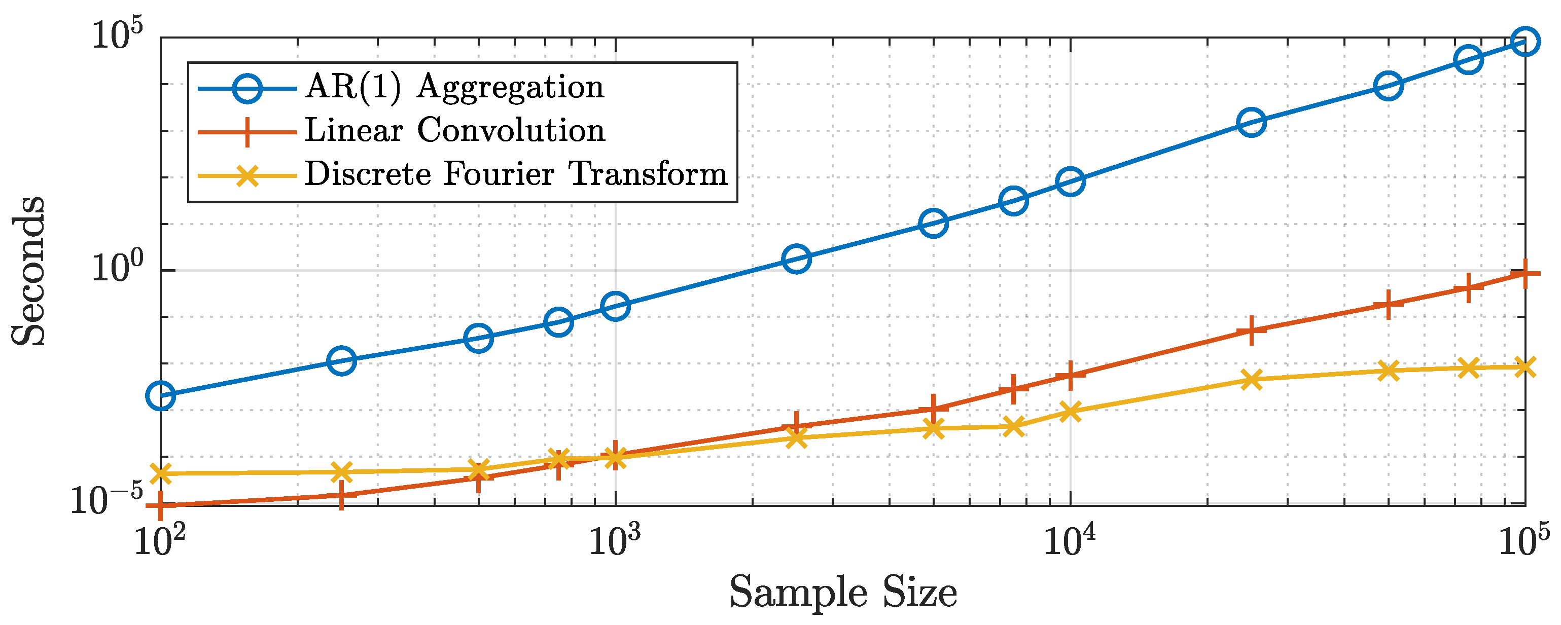
Figure 1 shows the computational times for a MATLAB implementation of the algorithms presented in this paper. The algorithms were run on a computer with an Intel Core i7-7820HQ at 2.90GHz running Windows 10 Enterprise and using the MATLAB 2019b release. Following the results of Haldrup and Vera-Valdés (2017), we generated the same number of $AR\left(1\right)$ processes as the sample size for the standard aggregation algorithm (6). To make fair comparisons, we used MATLAB’s built-in filter function to generate the individual $AR\left(1\right)$ processes and in the linear convolution algorithm. We generated the coefficients in the moving average representation using the recursive form instead of relying on the built-in Beta function, that is:

$${\varphi }_k=\frac{{(a+k-2)}^{1/2}}{{(a+k-2+b)}^{1/2}}{\varphi }_{k-1},$$

where ${\varphi }_0=1$.

The figure shows that the linear convolution and discrete Fourier transform algorithms are several times faster than aggregating independent $AR\left(1\right)$ processes for all sample sizes. In particular, the figure shows that generating long-range-dependent processes by aggregating $AR\left(1\right)$ series becomes computationally infeasible as the sample size increases. Regarding the two proposed methods, the figure shows that the discrete Fourier transform algorithm is faster than the linear convolution algorithm for sample sizes greater than 750 observations. Moreover, the relative performance of the discrete Fourier transform algorithm increases with the sample size.

Table 1. Computational times in seconds of the MATLAB implementation of the different algorithms to generate long-range dependence. $LC$ and $DFT$ stand for Linear Convolution and Discrete Fourier Transform, respectively. The reported times are the average of 100 replications for all sample sizes for the $LC$ and $DFT$ algorithms and for sample sizes up to 1000 for the $AR\left(1\right)$ aggregation algorithm. For larger sample sizes, the $AR\left(1\right)$ aggregation algorithm was computed once due to computational restrictions.

	$\mathit{T}={10}^2$	$\mathit{T}={10}^3$	$\mathit{T}={10}^4$	$\mathit{T}=5\times {10}^4$	$\mathit{T}={10}^5$
$AR\left(1\right)$ Agg.	$2.02\times {10}^{-3}$	$1.70\times {10}^{-1}$	$8.08\times {10}^1$	$9.23\times {10}^3$	$8.29\times {10}^4$
$LC$	$1.00\times {10}^{-5}$	$1.10\times {10}^{-4}$	$5.51\times {10}^{-3}$	$1.86\times {10}^{-1}$	$8.60\times {10}^{-1}$
$DFT$	$4.00\times {10}^{-5}$	$9.00\times {10}^{-5}$	$9.30\times {10}^{-4}$	$7.04\times {10}^{-3}$	$8.46\times {10}^{-3}$

presents a subset of the computational times for all algorithms considered.

It took approximately $0.17$ s to generate one long-range-dependent series of size $T={10}^3$ by aggregating independent $AR\left(1\right)$ processes, while more than 80 s to generate a sample of size $T={10}^4$. These computational times make it impractical to use this algorithm for Monte Carlo experiments or bootstrap procedures. The computational times for the discrete Fourier transform and the linear convolution algorithms were approximately the same for sample sizes of around ${10}^3$ observations. Nonetheless, the former was ${10}^2$-times faster than the latter for ${10}^5$ observations. These results suggested using the discrete Fourier transform to generate large samples of long-range-dependent processes by cross-sectional aggregation. Moreover, note that these results are much in line with the ones obtained by Jensen and Nielsen (2014) for the fractional difference operator. In this regard, the proposed algorithms to generate long-range dependence have similar computational requirements as those of the fractional difference operator. Codes implementing the discrete Fourier transform algorithm for long-range dependence generation by cross-sectional aggregation in R (

Listing A1. R Code.

csadiff <- function(x, a, b){

iT <- length(x)

n <- nextn(2*iT - 1, 2)

k <- 0:(iT-1)

coefs <- (beta(a+k,b)/beta(a,b))^(1/2)

csax <- fft(fft(c(x, rep(0, n - iT))) *

fft(c(coefs, rep(0, n - iT))), inverse = T) / n;

return(Re(csax[1:iT]))

}

) and MATLAB (

Listing A2. MATLAB code.

function [csax] = csa_diff(x,a,b)

iT = size(x,1);

n = 2.^nextpow2(2*iT-1);

coefs = ( beta(a+(0:iT-1),b) ./ beta(a,b) ).^(1/2);

csax = ifft(fft(x, n).*fft(coefs’, n));

csax = cx(1:iT, :);

end

) are available in Appendix B.

4. Nonfractional Long-Range Dependence and the Antipersistent Property

It is well known in the long memory literature that the fractional difference operator implies that the autocorrelation function is negative for negative degrees of the parameter d. The sign of the autocorrelation function for a fractionally differenced process, ${\gamma }_{I\left(d\right)}\left(k\right)$, depends on $\mathsf{\Gamma }\left(d\right)$ in the denominator, which is negative for $d\in (-1/2,0)$; see (3). Furthermore, let $x_t\sim I\left(d\right)$, and let $f_X\left(\lambda \right)$ be its spectral density, then:

$$f_X\left(\lambda \right)=\frac{{\sigma }^2}{2\pi }{\left|\sum _{k=0}^{\infty }{\pi }_k{e}^{-ik\lambda }\right|}^2=\frac{{\sigma }^2}{2\pi }{\left|1-e^{-i\lambda }\right|}^{-2d}\approx \frac{{\sigma }^2}{2\pi }{\lambda }^{-2d}\mathrm{as}\lambda \to 0,$$

(10)

where ${\pi }_k$ are given as in (2); see Beran et al. (2013). Thus, $f_X\left(\lambda \right)\to 0$ as $\lambda \to 0$ for $d\in (-1/2,0)$, that is the fractional difference operator for negative values of the parameter implies a spectral density collapsing to zero at the origin. Moreover, note that the behavior of the spectral density at the origin implies that the coefficients of the moving average representation of a fractionally differenced process with negative degree of long-range dependence sum to zero.

These properties have been named antipersistence in the literature. It is thus necessary to distinguish between long memory and antipersistence for fractionally differenced processes depending on the sign of the long-range dependence parameter. We argue that the antipersistent properties are a restriction imposed by the use of the fractional difference operator. In this regard, the restriction on the sum of the coefficients in the moving average representation may be too strict for real data. It takes but a small deviation on any of the infinite coefficients to violate this restriction, providing further evidence of the brittleness of fractionally differenced processes; see Veitch et al. (2013). We showed that $CSA(a,b)$ processes do not share these restrictions and are thus less brittle.

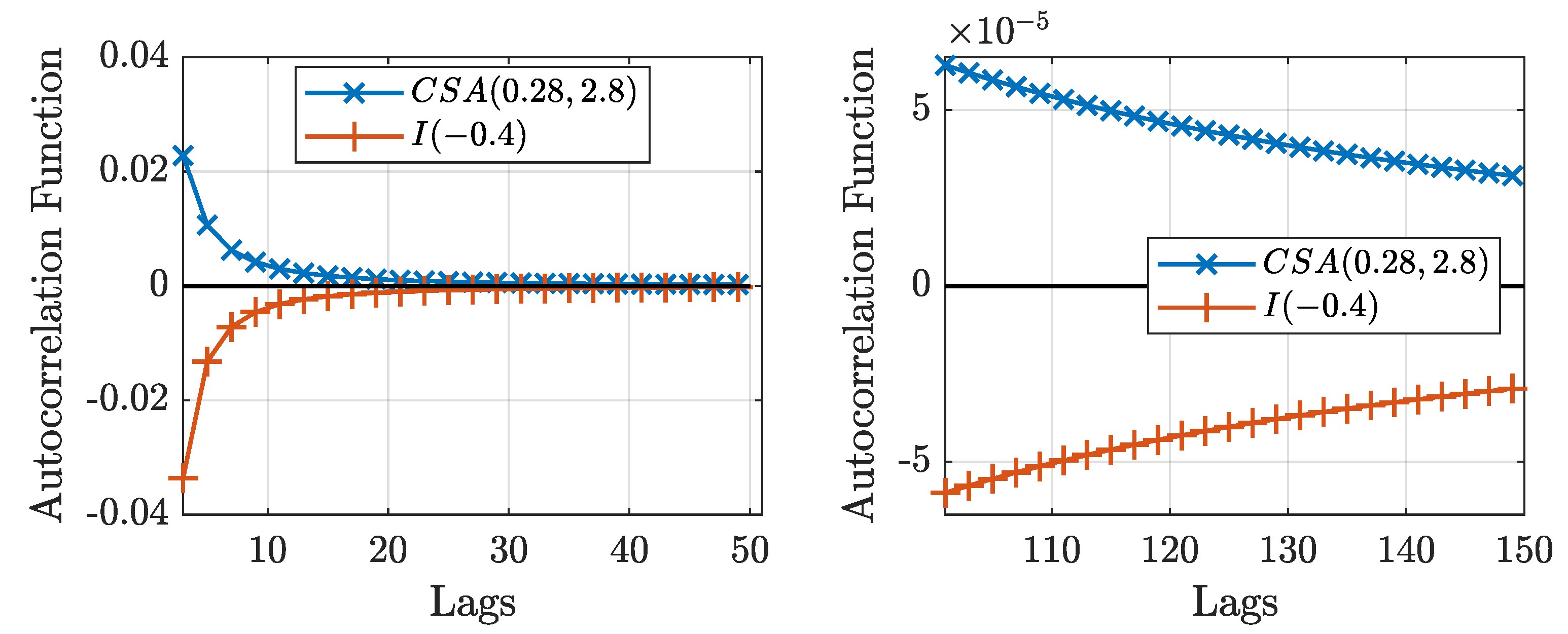
First, (7) demonstrates that the autocorrelation function for $CSA(a,b)$ processes only depends on the Beta function, which is always positive. Figure 2 shows the autocorrelation function for an $I(-0.4)$ process and a $CSA(0.28,2.8)$ process. The figure shows that both processes show the same rate of decay in their autocorrelation functions, but opposite signs.

Then, Theorem 2 proves that the spectral density for $CSA(a,b)$ processes with $b\in (2,3)$ converges to a positive constant as the frequency goes to zero.

Theorem 2.

Let $x_t\sim CSA(a,b)$ be defined as in (8) with $b\in (2,3)$, and let $f_X\left(\lambda \right)$ be its spectral density, then:

$$f_X\left(0\right)=c_{a,b}>0,$$

where $c_{a,b}$ depends on the parameters of the Beta distribution.

Proof. 

Let $x_t\sim CSA(a,b)$ be defined as in (8) with $a\in (0,3)$ and $b\in (2,3)$; the spectral density of $x_t$ at the origin is given by:

$$f_X\left(0\right)=\frac{{\sigma }^2}{2\pi }{\left|\sum _{k=0}^{\infty }{\varphi }_k\right|}^2,$$

where ${\varphi }_k=B{(a+k,b)}^{1/2}/B{(a,b)}^{1/2}$. Thus, $f_X\left(0\right)$ can be written as:

$$\begin{array}{cc}\hfill f_X\left(0\right)& =\frac{{\sigma }^2}{2\pi }{\left|\sum _{k=0}^{\infty }{\varphi }_k\right|}^2=\frac{{\sigma }^2}{2\pi B(a,b)}{\left|\sum _{k=0}^{\infty }B{(a+k,b)}^{1/2}\right|}^2=\frac{{\sigma }^2}{2\pi B(a,b)}{\left|\sum _{k=0}^{\infty }{\left[\frac{\mathsf{\Gamma }(a+k)\mathsf{\Gamma }\left(b\right)}{\mathsf{\Gamma }(a+k+b)}\right]}^{1/2}\right|}^2\hfill \\ \hfill & =\frac{{\sigma }^2\mathsf{\Gamma }\left(b\right)}{2\pi B(a,b)}{\left|\sum _{k=0}^{\infty }{\left[\frac{\mathsf{\Gamma }(a+k)}{\mathsf{\Gamma }(a+k+b)}\right]}^{1/2}\right|}^2=\frac{{\sigma }^2\mathsf{\Gamma }\left(b\right)}{2\pi B(a,b)}{\left|\sum _{k=0}^{\infty }{\left[k^{-b}+O\left(k^{-(b+1)}\right)\right]}^{1/2}\right|}^2\hfill \\ \hfill & =\frac{{\sigma }^2\mathsf{\Gamma }\left(b\right)}{2\pi B(a,b)}\sum _{k=0}^{\infty }\left[k^{-b}+O\left(k^{-(b+1/2)}\right)\right]<\infty ,\hfill \end{array}$$

where in the previous to last equality, we used the large k asymptotic formula for the ratios of Gamma functions:

$$\frac{\mathsf{\Gamma }(a+k)}{\mathsf{\Gamma }(a+k+b)}=k^{-b}\left[1+O\left(k^{-1}\right)\right],$$

(see Phillips (2009)) and the convergence of the series is guaranteed from the Euler–Riemann Zeta function. Moreover, note that all terms in the expression are positive.    □

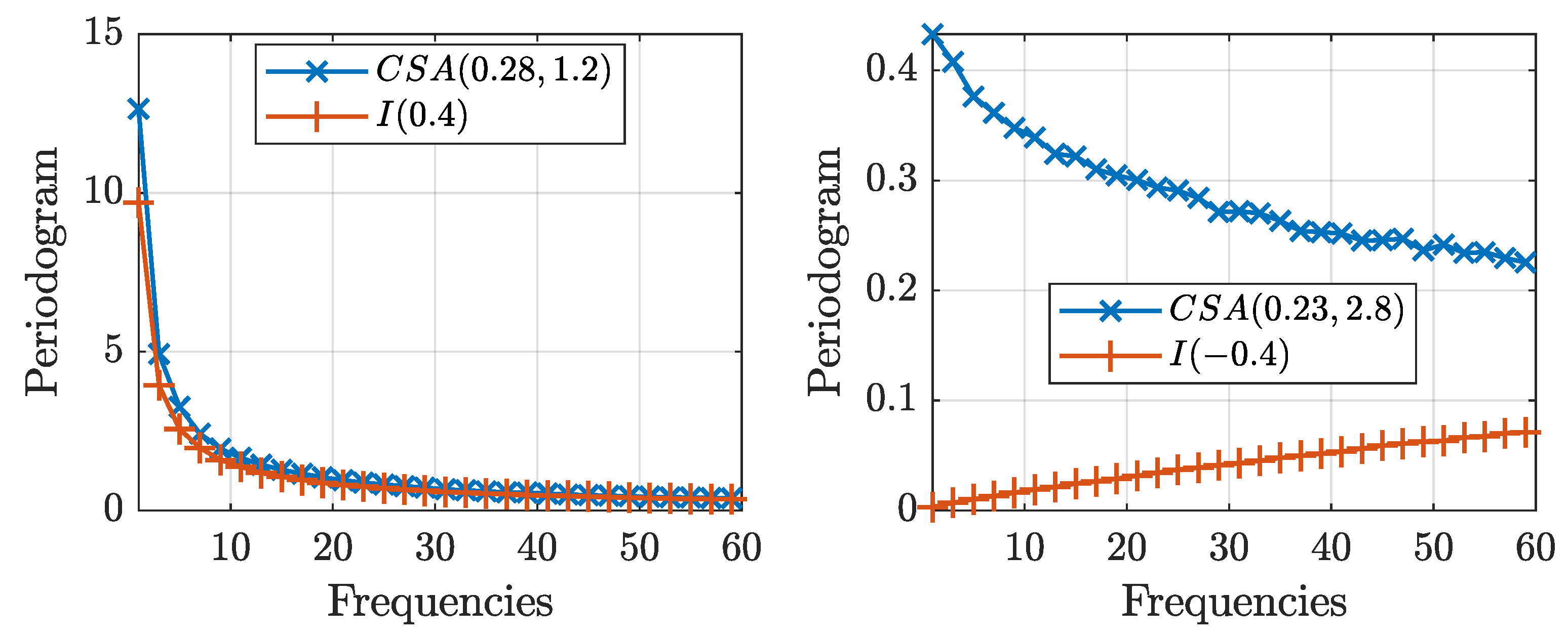
Figure 3 shows the periodogram, an estimate of the spectral density, for the $CSA(a,b)$ and $I\left(d\right)$ processes of size $T={10}^4$ averaged for ${10}^4$ replications. The figure shows that the periodograms for both processes exhibit similar behavior for positive values of the long-range dependence parameter, $d=1-b/2\in (0,1/2)$, diverging to infinity at the same rate. Nonetheless, for negative values of the long-range dependence parameter, $d=1-b/2\in (-1/2,0)$, the periodogram collapses to zero as the frequency goes to zero for $I\left(d\right)$ processes, while it converges to a constant for $CSA(a,b)$ processes. Following the discussion on the definitions for long memory in Haldrup and Vera-Valdés (2017), note that Theorem 2 implies that $CSA(a,b)$ processes with $b\in (2,3)$ are not long memory processes in the spectral sense. Nonetheless, $CSA(a,b)$ processes remain long-range-dependent in the covariance sense.

The behavior of the spectral density near zero has implications for estimation and inference. Pointedly, tests for long-range dependence in the frequency domain are affected. These types of tests are based on the behavior of the periodogram as the frequency goes to zero. Tests for long-range dependence in the frequency domain include the log-periodogram regression (see Geweke and Porter-Hudak (1983) and Robinson (1995b)) and the local Whittle approach (see Künsch (1987) and Robinson (1995a)).

On the one hand, the log-periodogram regression is given by:

$$log\left(I\left({\lambda }_k\right)\right)=c-2dlog\left({\lambda }_k\right)+u_k,k=1,\cdots ,m;$$

where $I\left({\lambda }_k\right)$ is the periodogram, ${\lambda }_k=e^{ik2\pi /T}$ are the Fourier frequencies, c is a constant, $u_k$ is the error term, and m is a bandwidth parameter that grows with the sample size. On the other hand, the local Whittle estimator minimizes the function:

$$R\left(H\right)=log\left(G\left(H\right)\right)-(2H-1)\frac{1}{m}\sum _{k=1}^{m}log\left({\lambda }_k\right),G\left(H\right)=\frac{1}{m}\sum _{k=1}^m{\lambda }_j^{2H-1}I\left({\lambda }_k\right),$$

where $H=d+1/2$ is the Hurst parameter, $I\left({\lambda }_k\right)$ is the periodogram, and m is the bandwidth. From (10), note that the log-periodogram regression provides an estimate of the long-range dependence parameter for $I\left(d\right)$ processes regardless of its sign. As Theorem 2 and Figure 3 show, these tests will be misspecified for $CSA(a,b)$ processes with $b\in (2,3)$.

To illustrate the misspecification problem,

Table 2. Mean and standard deviation (in parentheses) of estimated long-range dependence parameters by the $GPH$, $BR$, and $LW$ methods for the $CSA(a,b)$ and $I\left(d\right)$ processes where $b=2(1-d)$ so that they show the same degree of long-range dependence. Furthermore, the parameter a was selected following (12) below with $k=10$, and only a quadratic term was added for the bias-reduced method. We used the $MSE$ optimal bandwidth of $T^{4/5}$ (see Hurvich et al. (1998)) and a sample size of $T={10}^3$ with ${10}^4$ replications.

	$\mathit{d}=0.4$		$\mathit{d}=0.2$		$\mathit{d}=-0.2$		$\mathit{d}=-0.4$
	$\mathit{CSA}(\mathit{a},\mathit{b})$	$\mathit{I}\left(\mathit{d}\right)$	$\mathit{CSA}(\mathit{a},\mathit{b})$	$\mathit{I}\left(\mathit{d}\right)$	$\mathit{CSA}(\mathit{a},\mathit{b})$	$\mathit{I}\left(\mathit{d}\right)$	$\mathit{CSA}(\mathit{a},\mathit{b})$	$\mathit{I}\left(\mathit{d}\right)$
$GPH$	0.425	0.391	0.260	0.195	0.177	−0.194	0.211	−0.387
	(0.042)	(0.043)	(0.043)	(0.042)	(0.042)	(0.042)	(0.042)	(0.043)
$BR$	0.434	0.402	0.264	0.201	0.159	−0.198	0.172	−0.395
	(0.066)	(0.066)	(0.066)	(0.066)	(0.066)	(0.065)	(0.065)	(0.067)
$LW$	0.424	0.390	0.258	0.194	0.178	−0.196	0.213	−0.389
	(0.033)	(0.034)	(0.034)	(0.033)	(0.033)	(0.033)	(0.034)	(0.034)

reports the long-range dependence parameter estimated by the method of Geweke and Porter-Hudak 1983, $GPH$, the bias-reduced version of Andrews and Guggenberger 2003, $BR$, and the local Whittle approach by Künsch (1987), $LW$, for several values of the long-range dependence parameter for both fractionally differenced and cross-sectionally aggregated processes.

Table 2 shows that the estimator is relatively close to the true parameter for both processes when $d=1-b/2\in (0,1/2)$, if slightly overshooting it for the cross-sectionally aggregated process, as reported by Haldrup and Vera-Valdés (2017). This contrasts the $d=1-b/2\in (-1/2,0)$ case. The table shows that the estimator remains precise for the $I\left(d\right)$ series, while it incorrectly estimates a value $b\in (1,2)$ for the $CSA(a,b)$ processes. This is of course not surprising in light of Theorem 2.

In sum, the lack of the antipersistent property in $CSA(a,b)$ processes shows that care must be taken when estimating the long-range dependence parameters if the fractional difference operator does not generate the long-range dependence. We proved that wrong conclusions can be obtained when estimating the long-range dependence parameter using tests based on the frequency domain if the true nature of the long-range dependence is not the fractional difference operator. This result is particularly relevant in light of Granger’s argument of the fractional difference operator being in the “empty box” of econometric models that do not arise in the actual economy. To correctly estimate the long-range dependence parameter, the next section presents the maximum likelihood estimator, $MLE$, for the $CSA(a,b)$ processes.

5. Nonfractional Long-Range Dependence Estimation

Let $X={[x_0,\cdots ,x_{T-1}]}^{\prime }$ be a sample of size T of a $CSA(a,b)$ process, and let $\theta ={[a,b,{\sigma }^2]}^{\prime }$. Under the assumption that the error terms follow a normal distribution, X follows a normal distribution with the probability density given by:

$$f\left(\theta \right|X)={\left(2\pi \right)}^{-T/2}{\left|\Sigma \right|}^{-1/2}exp\left(-\frac{1}{2}{X}^{\prime }{\Sigma }^{-1}X\right),$$

where $\Sigma$ is given by:

$$\Sigma ={\sigma }^2{\gamma }_{CSA(a,b)}\left(0\right){\left[{\gamma }_{CSA(a,b)}\left(\right|j-k\left|\right)\right]}_{j,k=1}^T,$$

with ${\gamma }_{CSA(a,b)}\left(k\right)$ the autocorrelation function in (7).

Consider the log-likelihood function given by:

$$\mathcal{L}\left(\theta \right|X)=log(f\left(\theta \right|X\left)\right),$$

and estimate the parameters by:

$$\widehat{\theta }=\underset{\theta }{max}\mathcal{L}\left(\theta \right|X).$$

(11)

The standard asymptotic theory for maximum likelihood estimation, $MLE$, applies. We have the following theorem.

Theorem 3.

Let $X={[x_0,\cdots ,x_{T-1}]}^{\prime }$ be a sample of size T of a $CSA(a,b)$ process with normally distributed error terms, and let $\theta ={[a,b,{\sigma }^2]}^{\prime }$. Furthermore, let $\widehat{\theta }$ be given by (11). Then:

$$\mathit{plim}\widehat{\theta }=\theta ,$$

where $plim$ stands for the limit in probability.

Proof. 

Notice that ${\sigma }_1^2{\gamma }_{CSA(a_1,b_1)}\left(k\right)\ne {\sigma }_2^2{\gamma }_{CSA(a_2,b_2)}\left(k\right)$ for $a_1\ne a_2$, $b_1\ne b_2$, or ${\sigma }_1^2\ne {\sigma }_2^2$, which shows that the log-likelihood function is identified. Moreover, the log-likelihood function is continuous and twice differentiable. Thus, $MLE$ satisfies the standard regularity conditions, and it is thus a consistent estimator; see Davidson and MacKinnon (2004).    □

Theorem 3 shows that $MLE$ is a consistent estimator of the true parameters. Nonetheless, the finite sample properties may differ from the asymptotic ones, especially for smaller sample sizes (

Table 3. $MLE$ estimates of $CSA(a,b)$ processes. Standard deviations are shown in brackets. We used ${10}^3$ replications, and all random vector were sampled from an $\mathcal{N}(0,{\sigma }^2)$ distribution.

$(\mathit{a},\mathit{b},{\mathit{\sigma }}^2)$	$\mathit{T}=50$	$\mathit{T}={10}^2$	$\mathit{T}={10}^3$
$(0.2,1.2,1)$	$(0.403,1.772,0.870)$	$(0.344,1.599,0.873)$	$(0.247,1.239,0.896)$
	$[0.369,0.722,0.187]$	$[0.229,0.577,0.124]$	$[0.049,0.140,0.042]$
$(0.4,1.8,0.5)$	$(0.575,2.089,0.440)$	$(0.517,1.954,0.443)$	$(0.404,1.673,0.447)$
	$[0.481,0.755,0.095]$	$[0.320,0.661,0.063]$	$[0.089,0.230,0.021]$
$(1.2,2.2,1.5)$	$(0.993,1.864,1.365)$	$(1.233,2.155,1.336)$	$(1.202,2.219,1.351)$
	$[0.842,0.730,0.291]$	$[0.691,0.676,0.193]$	$[0.265,0.341,0.066]$
$(0.8,2.4,0.2)$	$(0.690,1.977,0.181)$	$(0.855,2.233,0.178)$	$(0.812,2.278,0.179)$
	$[0.649,0.728,0.039]$	$[0.492,0.667,0.025]$	$[0.171,0.336,0.009]$

). For implementation purposes, concentrating for ${\sigma }^2$ in the log-likelihood reduces the computational burden by reducing the number of parameters to estimate. Let $\Sigma ={\sigma }^2\mathsf{\Gamma }$, and differentiate the log-likelihood with respect to ${\sigma }^2$ to obtain:

$${\sigma }^2=T^{-1}{X}^{\prime }{\mathsf{\Gamma }}^{-1}X.$$

Thus, the concentrated log-likelihood is given by:

$${\mathcal{L}}_c\left({[a,b]}^{\prime }\right|X)=\frac{1}{2T}log\left|\mathsf{\Gamma }\right|+\frac{1}{2}log\left(T^{-1}{X}^{\prime }{\mathsf{\Gamma }}^{-1}X\right),$$

where we discarded the constant and divided by T to reduce the effect of the sample size on the convergence criteria. Hence, we estimate the parameters by:

$${[\widehat{a},\widehat{b}]}^{\prime }=\underset{a,b}{max}{\mathcal{L}}_c(X;a,b),$$

and the variance of the error term by:

$${\widehat{\sigma }}^2=T^{-1}{X}^{\prime }{\widehat{\mathsf{\Gamma }}}^{-1}X,$$

where we obtain $\widehat{\mathsf{\Gamma }}$ by substituting the values of $\widehat{a},\widehat{b}$.

Moreover, we used the recursive nature of the Beta function to reduce the computational burden. Table 3 presents a Monte Carlo experiment for the $MLE$. We used ${10}^3$ replications with sample sizes $T=50$, $T={10}^2$, and $T={10}^3$. As the table shows, the $MLE$ estimates become closer to the true values as the sample size increases, in line with Theorem 3.

6. Application

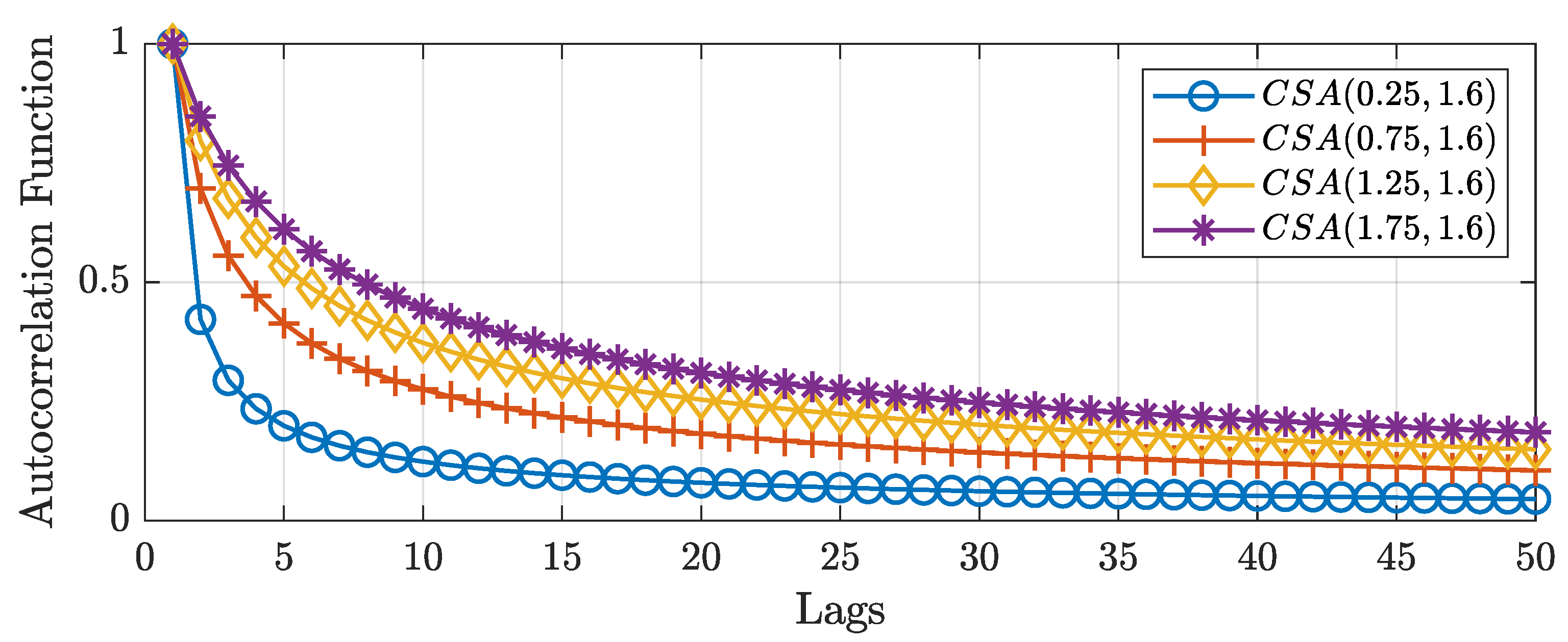
As an application, we show that we can use the extra flexibility of the cross-sectionally aggregated process to approximate a process generated using the fractional difference operator. Figure 4 shows the autocorrelation function of cross-sectional aggregated processes for different values of the first parameter of the Beta distribution. The figure shows that as the first parameter increases, so does the autocorrelation function for the initial lags, while maintaining the same long-term behavior. Hence, the first argument models the short-term dynamics. In this regard, cross-sectionally aggregated processes are capable of capturing both short- and long-term dynamics in a single theoretically based framework.

Consider the function given by:

$$L(k,a,d):=\sum _{j=0}^k{\left({\gamma }_{I\left(d\right)}\left(j\right)-{\gamma }_{CSA(a,2(1-d\left)\right)}\left(j\right)\right)}^2,$$

(12)

which measures the squared difference between autocorrelations at the first k lags for $CSA(a,b)$ and $I\left(d\right)$ processes with the same long-range dynamics. Minimizing (12) with respect to the parameter a, we find the $CSA(a,b)$ process that best approximates a long memory $I\left(d\right)$ process up to lag k, while having the same long-range dependence. Given the different forms of the autocorrelation functions, there is in general no value of the parameter a that minimizes (12) for all values of k. For instance, ${min}_a\mathcal{L}(2,a,0.2)=0.118$, while ${min}_a\mathcal{L}(30,a,0.2)=0.121$.

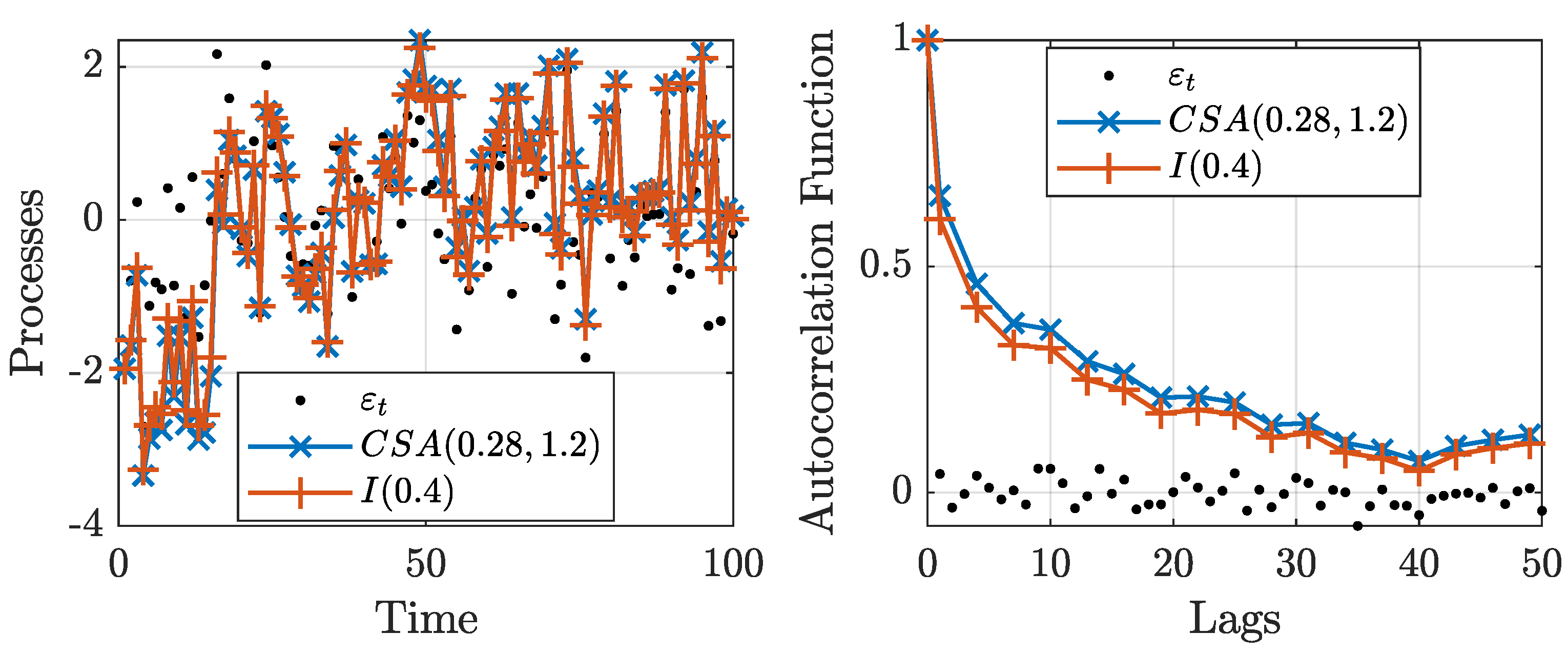
Nonetheless, selecting a medium-sized k, say $k=10$, the approximation turns out to be quite satisfactory in general. In Figure 5, we present a white noise process, ${\left\{{\epsilon }_t\right\}}_{t=1}^{{10}^3}\sim N(0,1)$, and long-range-dependent processes. These processes are obtained by using the fractional difference operator with parameter $d=0.4$ and using the cross-sectional aggregated algorithm with parameters $a=0.28$ and $b=1.2$.

The figure shows that the filtered series are almost identical. Moreover, the autocorrelation functions exhibit similar dynamics. In this context, the fractional difference operator can be viewed as another example of models that generate processes with similar properties to their theoretical explanations, but are not equivalent; see Portnoy (2019) for an example with the $AR\left(1\right)$ model. Thus, the figure shows that it is possible to generate cross-sectionally aggregated processes that closely mimic the ones due to fractional differencing while providing theoretical support for the presence of long-range dependence.

In real data, series such as inflation, output, and volatility have been shown to possess long-range dependence. One of the explanations behind the presence of the long-range dependence is cross-sectional aggregation; see Diebold and Rudebusch (1989), Balcilar (2004), and Altissimo et al. (2009). Climate data have also been shown to possess long-range dependence. Several authors have argued that aggregation may be the reason behind the presence of long-range dependence in temperature data; see Baillie and Chung (2002); Gil-Alana (2005); Mills (2007); Vera-Valdés (2021a).

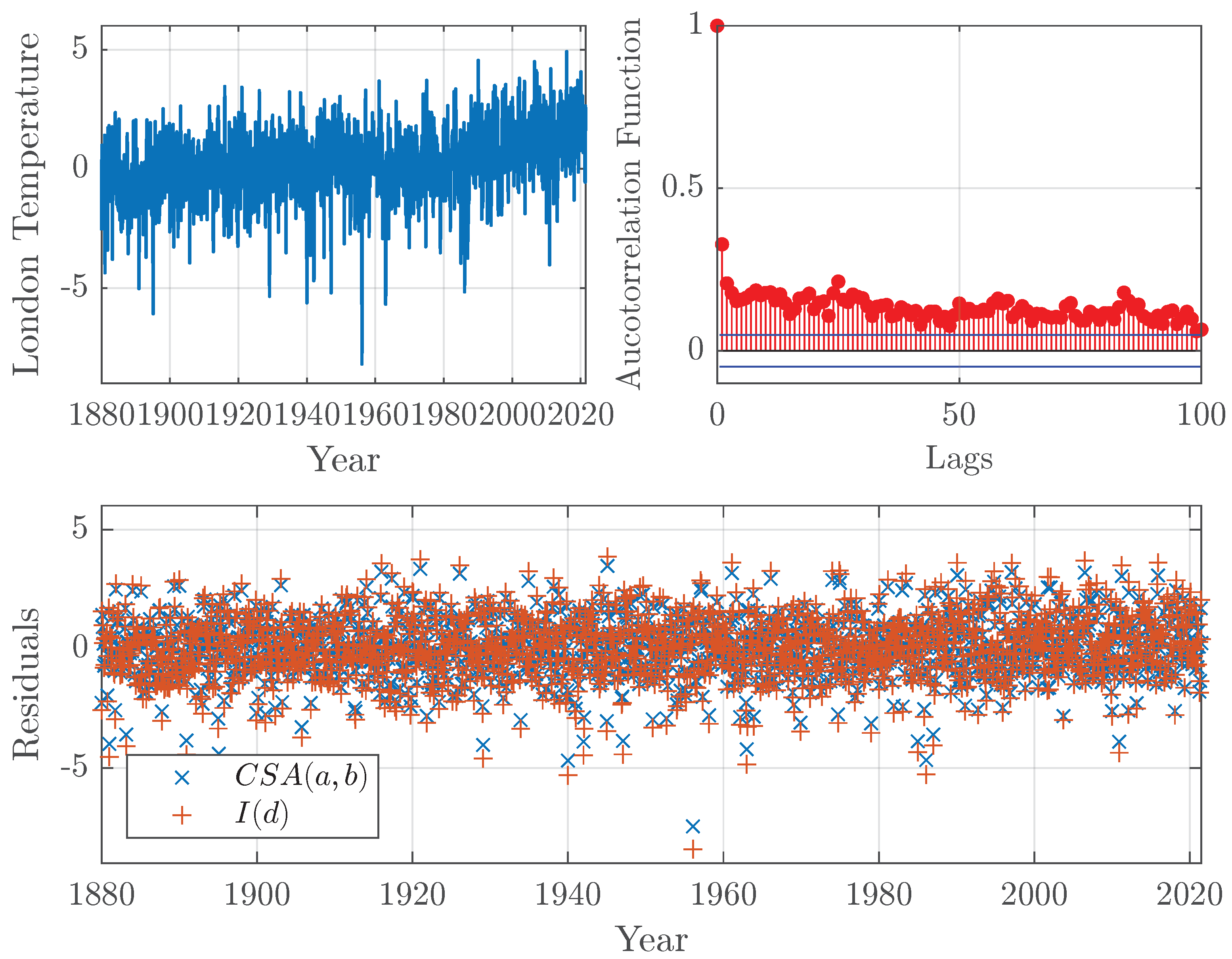
Figure 6 shows an example using temperature data. The data came from GISTEMP, an estimate of global surface temperature change constructed by the NASA Goddard Institute for Space Studies. GISTEMP specifies the temperature anomaly at a given location as the weighted average of the anomalies for all stations located in close proximity. The data are updated monthly and combine data from land and ocean surface temperatures; see GISTEMP (2020); Lenssen et al. (2019).

The figure shows temperature anomalies for the grid near London, the United Kingdom. The data possess long-range dependence, as seen in their autocorrelation function. To model the long-range dependence, we fit the $CSA(a,b)$ and $I\left(d\right)$ models to the data. On the one hand, the estimated long-range dependence parameter for the fractional difference model is $\widehat{d}=0.226$. On the other hand, the estimated parameters for the $CSA(a,b)$ model using the $MLE$ developed in Section 5 are $\widehat{a}=0.074$ and $\widehat{b}=1.229$, which correspond to a long-range dependence parameter of $0.385$. The residuals from the estimated models are also shown. Note that the residuals from the $CSA(a,b)$ model are, on average, smaller than the residuals from the $I\left(d\right)$ model. The residual sum squares for the $CSA(a,b)$ and $I\left(d\right)$ models are 2405 and 3076, respectively. The example shows that the $CSA(a,b)$ model extracts more of the dynamics in the data than the fractional difference operator. Hence, given how the data were generated, as the aggregation of temperature series at different stations, the $CSA(a,b)$ model provides a better, theoretically supported fit to the data.

7. Conclusions

Granger argued that fractionally integrated processes fall into the “empty box” category of theoretical developments that do not arise in the real economy. Moreover, Veitch et al. (2013) argued that “time series whose long-range dependence scaling derives directly from fractional differencing [...] are far from typical when it comes to their long-range dependence character”. Thus, this paper developed a long-range dependence framework based on cross-sectional aggregation, the most predominant theoretical explanation for the presence of long-range dependence in data. In this regard, this paper developed a framework to model long-range dependence that arises in the real economy, and it is thus not in the “empty box”.

This paper built on the long-range dependence literature by presenting two novel algorithms to generate long-range dependence by cross-sectional aggregation. The algorithms have a similar computational burden as the one for the fractional difference operator. They are exact in the sense that no approximation regarding the number of aggregating units is needed.

Moreover, we studied the antipersistent properties and proved that the autocorrelation function for $CSA(a,b)$ processes is positive, and the spectral density does not collapse to zero as the frequency goes to zero. We argued that the antipersistent properties are a restriction imposed by the use of the fractional difference operator. We showed that $CSA(a,b)$ processes do not share these restrictions, and are thus less brittle. The paper showed that the lack of antipersistence has implications for long-range dependence estimators in the frequency domain, which will be misspecified.

To solve the misspecification issue, we developed the maximum likelihood estimator for long-range dependence by cross-sectional aggregation to obtain a consistent estimator. Furthermore, we proposed to reduce the computational burden of the $MLE$ by taking advantage of the recursive nature of the autocorrelation function of cross-sectionally aggregated processes. As an application, we showed that cross-sectionally aggregated processes can approximate a fractionally differenced process.

Our results have implications for applied work with long-range-dependent processes where the source of the long-range dependence is cross-sectional aggregation. We showed on an example using temperature data that the model provides a better fit to the data than the fractional difference operator. We argued that cross-sectionally aggregation is a clear theoretical justification for the presence of long range-dependence. In this regard, this paper backs the case of Portnoy (2019) to employ models only when the underlying model assumptions have clear and convincing scientific justification.

References

- Adenstedt, Rolf K. 1974. On Large-Sample Estimation for the Mean of a Stationary Random Sequence. The Annals of Statistics 2: 1095–107. [Google Scholar] [CrossRef]
- Altissimo, Filippo, Benoit Mojon, and Paolo Zaffaroni. 2009. Can Aggregation Explain the Persistence of Inflation? Journal of Monetary Economics 56: 231–41. [Google Scholar] [CrossRef]
- Andrews, Donald W. K., and Patrik Guggenberger. 2003. A Bias-Reduced Log-Periodogram Regression Estimator For The Long-Memory Parameter. Econometrica 71: 675–712. [Google Scholar] [CrossRef]
- Baillie, Richard T. 1996. Long Memory Processes and Fractional Integration in Econometrics. Journal of Econometrics 73: 5–59. [Google Scholar] [CrossRef]
- Baillie, Richard T., Fabio Calonaci, Dooyeon Cho, and Seunghwa Rho. 2019. Long Memory, Realized Volatility and Heterogeneous Autoregressive Models. Journal of Time Series Analysis, 1–20. [Google Scholar] [CrossRef]
- Baillie, Richard T., and Sang Kuck Chung. 2002. Modeling and forecasting from trend-stationary long memory models with applications to climatology. International Journal of Forecasting 18: 215–26. [Google Scholar] [CrossRef]
- Balcilar, Mehmet. 2004. Persistence in Inflation: Does Aggregation Cause Long Memory? Emerging Markets Finance and Trade 40: 25–56. [Google Scholar] [CrossRef]
- Beran, Jan, Yuanhua Feng, Sucharita Ghosh, and Rafal Kulik. 2013. Long-Memory Processes: Probabilistic Theories and Statistical Methods. Berlin/Heidelberg, Germany: Springer. [Google Scholar] [CrossRef]
- Bhardwaj, Geetesh, and Norman R. Swanson. 2006. An Empirical Investigation of the Usefulness of ARFIMA Models for Predicting Macroeconomic and Financial Time Series. Journal of Econometrics 131: 539–78. [Google Scholar] [CrossRef] [Green Version]
- Chevillon, Guillaume, Alain Hecq, and Sébastien Laurent. 2018. Generating Univariate Fractional Integration Within a Large VAR(1). Journal of Econometrics 204: 54–65. [Google Scholar] [CrossRef]
- Cooley, James W., Peter A. W. Lewis, and Peter D. Welch. 1969. The Fast Fourier Transform and its Applications. IEEE Transactions on Education 12: 27–34. [Google Scholar] [CrossRef] [Green Version]
- Davidson, Russell, and James G. MacKinnon. 2004. Econometric Theory and Methods. Oxford: Oxford University Press. [Google Scholar]
- Diebold, Francis X., and Glenn D. Rudebusch. 1989. Long Memory and Persistence in Agregate Output. Journal of Monetary Economics 24: 189–209. [Google Scholar] [CrossRef] [Green Version]
- Ergemen, Yunus Emre, Niels Haldrup, and Carlos Vladimir Rodríguez-Caballero. 2016. Common long-range dependence in a panel of hourly Nord Pool electricity prices and loads. Energy Economics 60: 79–96. [Google Scholar] [CrossRef]
- Geweke, John, and Susan Porter-Hudak. 1983. The Estimation and Application of Long Memory Time Series Models. Journal of Time Series Analysis 4: 221–38. [Google Scholar] [CrossRef]
- Gil-Alana, Luis A. 2005. Statistical modeling of the temperatures in the Northern Hemisphere using fractional integration techniques. Journal of Climate 18: 5357–69. [Google Scholar] [CrossRef]
- GISTEMP. 2020. GISS Surface Temperature Analysis (GISTEMP), Version 4. Available online: https://data.giss.nasa.gov/gistemp/ (accessed on 30 August 2021).
- Granger, Clive W. J. 1966. The Typical Spectral Shape of an Economic Variable. Econometrica 34: 150–61. [Google Scholar] [CrossRef]
- Granger, Clive W. J. 1980. Long Memory Relationships and the Aggregation of Dynamic Models. Journal of Econometrics 14: 227–38. [Google Scholar] [CrossRef]
- Granger, Clive W. J. 1999. Aspects of Research Strategies for Time Series Analysis. In Presentation to the Conference on New Developments in Time Series Economics. New Haven: Yale University. [Google Scholar]
- Granger, Clive W. J., and Roselyne Joyeux. 1980. An Introduction to Long Memory Time Series Models and Fractional Differencing. Journal of Time Series Analysis 1: 15–29. [Google Scholar] [CrossRef]
- Haldrup, Niels, and J. Eduardo Vera-Valdés. 2017. Long Memory, Fractional Integration, and Cross-Sectional Aggregation. Journal of Econometrics 199: 1–11. [Google Scholar] [CrossRef] [Green Version]
- Hassler, Uwe, and Barbara Meller. 2014. Detecting multiple breaks in long memory the case of U.S. inflation. Empirical Economics 46: 653–80. [Google Scholar] [CrossRef] [Green Version]
- Hosking, Jonathan R. M. 1981. Fractional Differencing. Biometrika 68: 165–76. [Google Scholar] [CrossRef]
- Hurvich, Clifford M., Rohit Deo, and Julia Brodsky. 1998. The Mean Squared Error of Geweke and Porter-Hudak’s Estimator of the Memory Parameter of a Long-Memory Time Series. Journal of Time Series Analysis 19: 19–46. [Google Scholar] [CrossRef]
- Jensen, Andreas Noack, and Morten Ørregaard Nielsen. 2014. A Fast Fractional Difference Algorithm. Journal of Time Series Analysis 35: 428–36. [Google Scholar] [CrossRef] [Green Version]
- Künsch, Hans. 1987. Statistical Aspects of Self-Similar Processes. Bernouli 1: 67–74. [Google Scholar]
- Lenssen, Nathan J. L., Gavin A. Schmidt, James E. Hansen, Matthew J. Menne, Avraham Persin, Reto Ruedy, and Daniel Zyss. 2019. Improvements in the GISTEMP Uncertainty Model. Journal of Geophysical Research: Atmospheres 124: 6307–26. [Google Scholar] [CrossRef]
- Linden, Mikael. 1999. Time Series Properties of Aggregated AR(1) Processes with Uniformly Distributed Coefficients. Economics Letters 64: 31–36. [Google Scholar] [CrossRef]
- Mills, Terence C. 2007. Time series modeling of two millennia of northern hemisphere temperatures: Long memory or shifting trends? Journal of the Royal Statistical Society. Series A: Statistics in Society 170: 83–94. [Google Scholar] [CrossRef]
- Oppenheim, Alan V., and Ronald W. Schafer. 2010. Discrete-Time Signal Processing. London: Pearson. [Google Scholar]
- Oppenheim, Georges, and Marie Claude Viano. 2004. Aggregation of Random Parameters Ornstein-Uhlenbeck or AR Processes: Some Convergence Results. Journal of Time Series Analysis 25: 335–50. [Google Scholar] [CrossRef]
- Osterrieder, Daniela, Daniel Ventosa-Santaulària, and J. Eduardo Vera-Valdés. 2019. The VIX, the Variance Premium, and Expected Returns. Journal of Financial Econometrics 17: 517–58. [Google Scholar] [CrossRef] [Green Version]
- Phillips, Peter C. B. 2009. Long Memory and Long Run Variation. Journal of Econometrics 151: 150–58. [Google Scholar] [CrossRef] [Green Version]
- Portnoy, Stephen. 2019. Edgeworth’s Time Series Model: Not AR(1) but Same Covariance Structure. Journal of Econometrics 213: 281–88. [Google Scholar] [CrossRef]
- Robinson, Peter M. 1978. Statistical Inference for a Random Coefficient Autoregressive Model. Scandinavian Journal of Statistics 5: 163–68. [Google Scholar] [CrossRef]
- Robinson, Peter M. 1995a. Gaussian Semiparametric Estimation of Long Range Dependence. The Annals of Statistics 23: 1630–61. [Google Scholar] [CrossRef]
- Robinson, Peter M. 1995b. Log-Periodogram Regression of Time Series with Long Range Dependence. The Annals of Statistics 23: 1048–72. [Google Scholar] [CrossRef]
- Veitch, Darryl, Anders Gorst-Rasmussen, and Andras Gefferth. 2013. Why FARIMA Models are Brittle. Fractals 21: 1–12. [Google Scholar] [CrossRef] [Green Version]
- Vera-Valdés, J. Eduardo. 2021a. Temperature Anomalies, Long Memory, and Aggregation. Econometrics 9: 9. [Google Scholar] [CrossRef]
- Vera-Valdés, J. Eduardo. 2021b. The persistence of financial volatility after COVID-19. Finance Research Letters. [Google Scholar] [CrossRef]
- Vera-Valdés, J. Eduardo. 2020. On long memory origins and forecast horizons. Journal of Forecasting 39: 811–26. [Google Scholar] [CrossRef] [Green Version]
- Zaffaroni, Paolo. 2004. Contemporaneous Aggregation of Linear Dynamic Models in Large Economies. Journal of Econometrics 120: 75–102. [Google Scholar] [CrossRef]
Figure 1.
Computational times at several sample sizes for a MATLAB implementation of the algorithms. Axes are logarithmic. The reported times are the average of 100 replications for all sample sizes for the linear convolution and discrete Fourier transform algorithms and for sample sizes up to 1000 for the aggregation algorithm. For larger sample sizes, the aggregation algorithm was computed once due to computational restrictions.
Figure 2.
Autocorrelation functions for an process and a one. The right plot shows lags 100 to 150.
Figure 3.
Mean periodograms of the and processes for long-range dependence parameters (left) and (right). A sample size of was used and replications.
Figure 4.
Autocorrelation function for a processes for different values of the parameter a while having the same asymptotic behavior.
Figure 5.
White noise series, , and filtered processes using cross-sectional aggregation, , and the fractional difference operator, (left). Autocorrelation functions for the white noise series and filtered processes (right).
Figure 6.
London temperature anomalies obtained from GISTEMP (top left) and its autocorrelation function (top right). Residuals from fitted and models to the series (bottom).