A Modeling Framework to Frame a Biological Invasion: Impatiens glandulifera in North America

Abstract

Biological invasions are a major component of global environmental change with severe ecological and economic consequences. Since eradicating biological invaders is costly and even futile in many cases, predicting the areas under risk to take preventive measures is crucial. Impatiens glandulifera is a very aggressive and prolific invasive species and has been expanding its invasive range all across the Northern hemisphere, primarily in Europe. Although it is currently spread in the east and west of North America (in Canada and USA), studies on its fate under climate change are quite limited compared to the vast literature in Europe. Hybrid models, which integrate multiple modeling approaches, are promising tools for making projections to identify the areas under invasion risk. We developed a hybrid and spatially explicit framework by utilizing MaxEnt, one of the most preferred species distribution modeling (SDM) methods, and we developed an agent-based model (ABM) with the statistical language R. We projected the I. glandulifera invasion in North America, for the 2020–2050 period, under the RCP 4.5 scenario. Our results showed a predominant northward progression of the invasive range alongside an aggressive expansion in both currently invaded areas and interior regions. Our projections will provide valuable insights for risk assessment before the potentially irreversible outcomes emerge, considering the severity of the current state of the invasion in Europe.

1. Introduction

Global environmental change is an ongoing and anthropogenic issue involving various components [1]. Biological invasions, together with climate change, are the leading drivers [2,3] of severe ecological consequences such as species extinctions, which are irreversible, and biodiversity loss, which takes millions of years to return to the former levels known from the periods following big extinction events, according to fossil records [4,5]. An invasive species causes, or is likely to cause, ecological and economic consequences alongside harm to human and animal well-being [6,7,8]. Ecosystem impacts caused by biological invasions, such as altering the function and structure of ecosystems [9], homogenization of biotas [10,11], and changing disturbance regimes [12,13,14], are diverse in severity and sometimes idiosyncratic [15]. Economic costs are also tremendous [16] and are expected to rise [17]. The impacts on ecosystem services [18], and especially threats to food security, constitute an important source of concern [19].

Today, invasive species introductions continue to increase without any sign of saturation worldwide [20]. In the face of this ever-growing problem, the most important lessons learned from the long history of biological invasions can be summarized as: the eradication of an established biological invader is virtually impossible [21], prevention is the most effective strategy [22], and the first step of prevention is to identify high-risk areas [23]. Consequently, model projections for potential range expansions play a crucial role in the prevention and controlling of biological invasions, since they can serve as early warning systems [24].

Over the last decades, owing to the increasing computational power and availability of biogeographic [25] and environmental data [26,27], correlative species distribution models (SDMs) have become widely popular due to their ability to produce credible, defensible, and repeatable information for conservation, management, and risk assessment [28,29,30]. Biological invasions have been a major application field of SDMs to be utilized for making two types of projections: the determination of the areas under invasion risk and prediction of the possible outcomes of an invasion under environmental change [31,32] via their spatial and temporal transferability [33]. Despite a vast number of studies involving different SDM methods, some of which with strategies to improve the results [34,35,36,37], the applicability of SDMs on biological invasions has been a source of controversy due to the potential violation of the basic assumptions of equilibrium, niche conservatism, and lack of dispersal limitation [38]. Hybrid modeling, the integration of distinct modeling approaches to represent complex, integrated systems [39,40], stands out as an alternative for modeling biological invasions to overcome the inherent limitations of SDMs [31,41,42] and incorporate the processes and interactions that SDMs cannot address to make more reliable projections with various promising examples [43,44,45,46]. Agent-based models (ABMs), which simulate populations or systems of populations as being composed of discrete agents [47] and have been used in many biological invasion studies [48,49,50,51], are a useful potential component for such hybrid models. In this regard, a hybrid model, which consists of SDM and ABM, can be highly useful in simulating biological invasions. While SDM provides suitability layers to be utilized by ABM, ABM simulates the essential processes such as dispersal, establishment, and biotic relations.

Impatiens glandulifera is native to the Western Himalayas and is considered one of the most prolific invasive species across the Northern Hemisphere [52]. It was introduced to Europe in the first half of the 19th century as an ornamental garden plant and for its high-quality nectar to be used in beekeeping [53,54]. While its primary habitats in the native range are forests and forest gaps [55], it primarily invades riparian habitats and only in recent decades has it been observed to colonize forests [56]. As rivers and water streams are its main dispersal vectors, anthropogenic means and animals are also known contributors to its seed dispersal [57].

Although I. glandulifera is defined as a transformer species [58], conclusions about its impact on species composition, diversity, and richness vary from “insignificant” [59,60,61] to “prominent” [62,63,64,65,66]. However, the differences can be attributed to factors such as the initial conditions of the invasion sites [67], the residence time in the invasion site [68], and local species composition [62]. Among other problems, I. glandulifera may cause erosion [69] due to its extremely shallow root system [70], increased eutrophication risk as a result of erosion [58], and problems related to stream management [53,59].

The invasive range of I. glandulifera currently extends across the Northern Hemisphere due to the combined effects of factors such as its wide environmental tolerance, the release from coevolved natural enemies [71,72], and opportunities caused by anthropogenic-land-use change [56]. Its invasive range in the Southern Hemisphere somewhat mirrors the northern pattern by the equator. I. glandulifera occurrence is currently recorded in more than 40 countries and registered as invasive in 30 countries [73].

Currently, the invasive range of I. glandulifera in North America is mainly concentrated in the Great Lakes, New England, and Canadian Maritimes regions in the East, Pacific Northwest, and British Columbia, along with Alaska and California as latitudinal extremes in the West. Occurrences are reported in at least 15 states in the U.S.A. and all provinces of Canada [73,74,75,76,77], and the species is considered “naturalized” in several of them [70,78,79]. The earliest records in North America date back to 1883 in Norwich, Connecticut [80]; 1901 in Ottawa, Ontario [70]; and 1912 in Port Huron, Michigan [81] in the East and 1937 in Burnaby, British Columbia [70]; and 1944 in Washington State [79] in the West. Its first occurrence in Alaska, where it is considered naturalized, was as recent as 2004 [82]. Despite its known presence in Mexico, occurrence records are not available through online databases [75,83]. Yet, for North America, literature on I. glandulifera is quite limited ([70,80] are some examples) compared to the vast number of studies for Europe (e.g., [53,66,84,85,86,87,88]). Consequently, there is still much to be understood about the fate of I. glandulifera in North America under climate change, considering the history and severity of the current state of the invasion in Europe.

We developed a hybrid and spatially explicit framework that consists of: (i) a correlative component (CC) utilizing species distribution modeling and (ii) an agent-based component (ABC) using agent-based modeling methods. These components are highly interconnected and work in a loop. In this loop, ABC is responsible for the generation, dispersal, and constraining of the establishment of agents in a dynamic heterogeneous environment, and CC uses these agents as occurrences to produce bioclimatic suitability layers. The occurrence of an invasion is only possible with the proper combination of the conditions in the recipient region [89], which is coined with the concept of invasion windows [90]. Additionally, the invasion law of minimum states that the least favorable one can be the determinant that makes the timing of introduction crucial alongside the place of introduction in a dynamic environment, since the invasion’s success is dependent on multiple factors [91,92]. Accordingly, while the framework proceeds in yearly time steps, the established success of agents relies on the invasion windows that are simulated via the environmental data layers. For the implementation presented here, we constructed species-specific procedures for ABC and utilized MaxEnt, one of the most preferred SDM methods [93], in the CC. This study aimed to project the I. glandulifera invasion in North America for the period 2020–2050 under the RCP 4.5 scenario and provide continental scale projections for an overview of the potential range expansion. Our projections will be one of the few studies conducted on I. glandulifera in North America, and thus will be a valuable contribution to the literature in addition to providing synoptic insights for preventive management, control, and conservation plans.

2. Materials and Methods

The framework was developed with the statistical language R (R version; 3.6.1, [94]) in the RStudio development environment (RStudio version; 1.2.1335, [95]). The MaxEnt algorithm was incorporated into the framework with the MaxEnt software for modeling species niches and distributions [96] via the Dismo package in R [97].

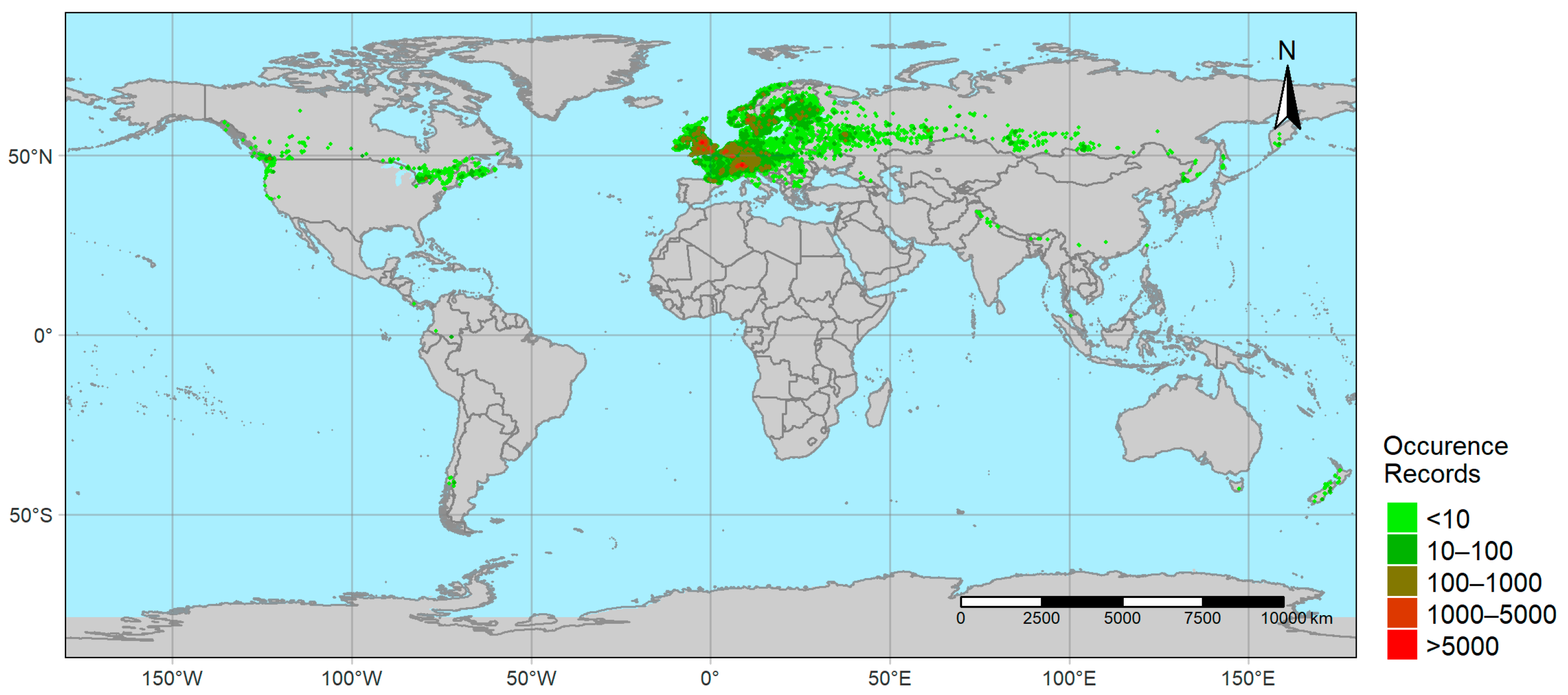
2.1. Occurrence Data

Occurrence records of I. glandulifera were obtained from the website of the Global Biodiversity Information Facility (GBIF) [98]. The data were cleaned by excluding the duplicate records and records without georeferencing and was filtered to contain only the observational data on the “basis of record” criteria (recorded as “human observation” in the basisOfRecord column). With this step, more than 300,000 occurrence records globally and 1522 from the region of interest, North America (respectively Occ_Global and Occ_NA hereafter), were obtained (Figure 1). While Occ_NA was used as the input for the simulations for correlative model training and initial agent generation, Occ_Global was utilized during the determination of the values of ABC variables.

2.2. Environmental Data Layers

Environmental layers can be categorized into three types: static, yearly, and emergent. Static environmental layers contain the data, which are assumed to be unchanged over the study period, such as elevation, slope, and soil pH. The yearly environmental data layers were pre-calculated for the years in the simulation period to be used in the corresponding time steps (e.g., climatic and land use data layers). Lastly, the emergent layers, unlike the static and yearly layers, were generated by the framework during the simulations, such as occurrence maps and climatic suitability maps.

2.2.1. Climatic Data Layers

The raw climatic dataset constitutes the basis of all climatic layers used in the model. It contains daily maximum temperature, minimum temperature, and precipitation for the period between 1990 and 2050, with a spatial resolution of 0.25°.

The raw climate dataset was constructed from two data sets to cover historical data and projections. The historical part was the ERA5 climate reanalysis data set [99] of the European Centre for Medium-Range Weather Forecasts (ECMWF), obtained from the Copernicus Climate Change Service Data Store [100]. The projections part was the downscaled projections under the RCP 4.5 scenario of MIROC5 General Circulation Model (GCM) [101], included in The NASA Earth Exchange Global Daily Downscaled Projections (NEX-GDDP) dataset [102,103]. Linear scaling, a common method to minimize the bias between GCM outputs and observed data, was applied to the projections to make these two data sets compatible [104,105]. Yearly bioclimatic variable (BCY) data layers, long-term bioclimatic variable (BCL) data layers, and accumulated chilling hours (ACHs) data layers were derived from the raw climatic data set.

BCY data layers were calculated from temporally upscaled (from daily to monthly) climatic raw data for the period of 1990–2050 via the Dismo package in R [97]. Then, the 30-year means were calculated from BCYs for the period 2020–2050 to obtain long-term bioclimatic variable data layers, and each layer was named with the last year of the period (e.g., BCL₂₀₂₀ is the mean of BCYs between 1991 to 2020).

Bioclimatic variables were selected based on the permutation importance, a measure that depended on the final MaxEnt model instead of the path to obtain the model itself, and it determined the contribution of each variable by permuting the values of the variables among the presence and background training points by measuring the decrease in the training area under the curve (AUC) [106]. This operation was conducted via the ENMeval package of R [107]. The block method was selected for spatial partitioning because of its known merits in cases involving temporal and spatial transfer [107].

Based on the mean permutation importance for each bioclimatic variable, which was calculated from the results of 50 repetitions conducted with Occ_NA and BCL₂₀₂₀, eight bioclimatic variables with a sum of 87.57% permutation importance were determined to narrow down the BCY and BCL: BIO13 (Precipitation of Wettest Month), BIO11 (Mean Temperature of Coldest Quarter), BIO15 (Precipitation Seasonality), BIO1 (Annual Mean Temperature), BIO9 (Mean Temperature of Driest Quarter), BIO6 (Min Temperature of Coldest Month), BIO18 (Precipitation of Warmest Quarter), and BIO4 (Temperature Seasonality). Permutation importance percentages of predictors are given in the Supplementary Materials, Table S1.

The ACHs in the February–March period (from day-of-year 32 to 90) were calculated for the period of 2005–2020 to construct the ACH data layers with a base temperature of 5 °C. Since chill hours calculations require hourly data, the temporal resolution of raw daily climatic data was temporally downscaled (from daily to hourly) via the chillR package in R [108].

2.2.2. Land Use Data Layers

Land use layers were derived from The Land-Use Harmonization 2 (LUH2) datasets for RCP 4.5 scenarios, with a spatial resolution of 0.25° [109,110]. Yearly layers were composited with the five classes of agricultural projections, including C3 annual crops, C3 nitrogen-fixing crops, C3 perennial crops, C4 annual crops, and C4 perennial crops.

2.2.3. Elevation and Slope Data Layers

The Median Statistic product with a 15 arc seconds resolution, from Global Multi-resolution Terrain Elevation Data 2010 (GMTED2010), developed by The U.S. Geological Survey (USGS) and the National Geospatial-Intelligence Agency (NGA), was selected as the elevation layer and downloaded from the Earth Resources Observation and Science (EROS) Center [111,112]. The slope layer was derived from the elevation layer via the terrain function of the raster package in R [113].

2.2.4. Soil pH Data Layers

Soil pH data at a depth of 0.15 m with a 7.5 arc seconds resolution was obtained from SoilGrids—a data set generated at the International Soil Reference and Information Centre (ISRIC)—to be utilized as the soil pH layer [114,115].

2.3. Structure of the Framework

As aforementioned, the framework consists of an ABC and a CC. The ABC generates and evaluates the agent populations to be utilized as occurrence records for model training by the CC. The CC makes projections for the ABC to be utilized as bioclimatic suitability layers. The processes of both components operate in a loop that spans consecutive time steps during the simulations (Figure 2). In a hierarchical sense, the CC primarily works at the population level by making projections based on the productive agent populations, while the ABC operates at the individual level by generating and processing agents.

2.3.1. Correlative Component

The CC performs model training with the long-term climatic conditions, which gradually change throughout the simulation period, and the latest occurrence is recorded to make projections for the upcoming year. Accordingly, BCL and the productive agent population of the previous time step are used to train a MaxEnt model as predictors and occurrence records, respectively. Then, the trained MaxEnt model is transferred to the BCY of the current time step to make projections in the form of bioclimatic suitability (BCS) layers, which the ABC will utilize.

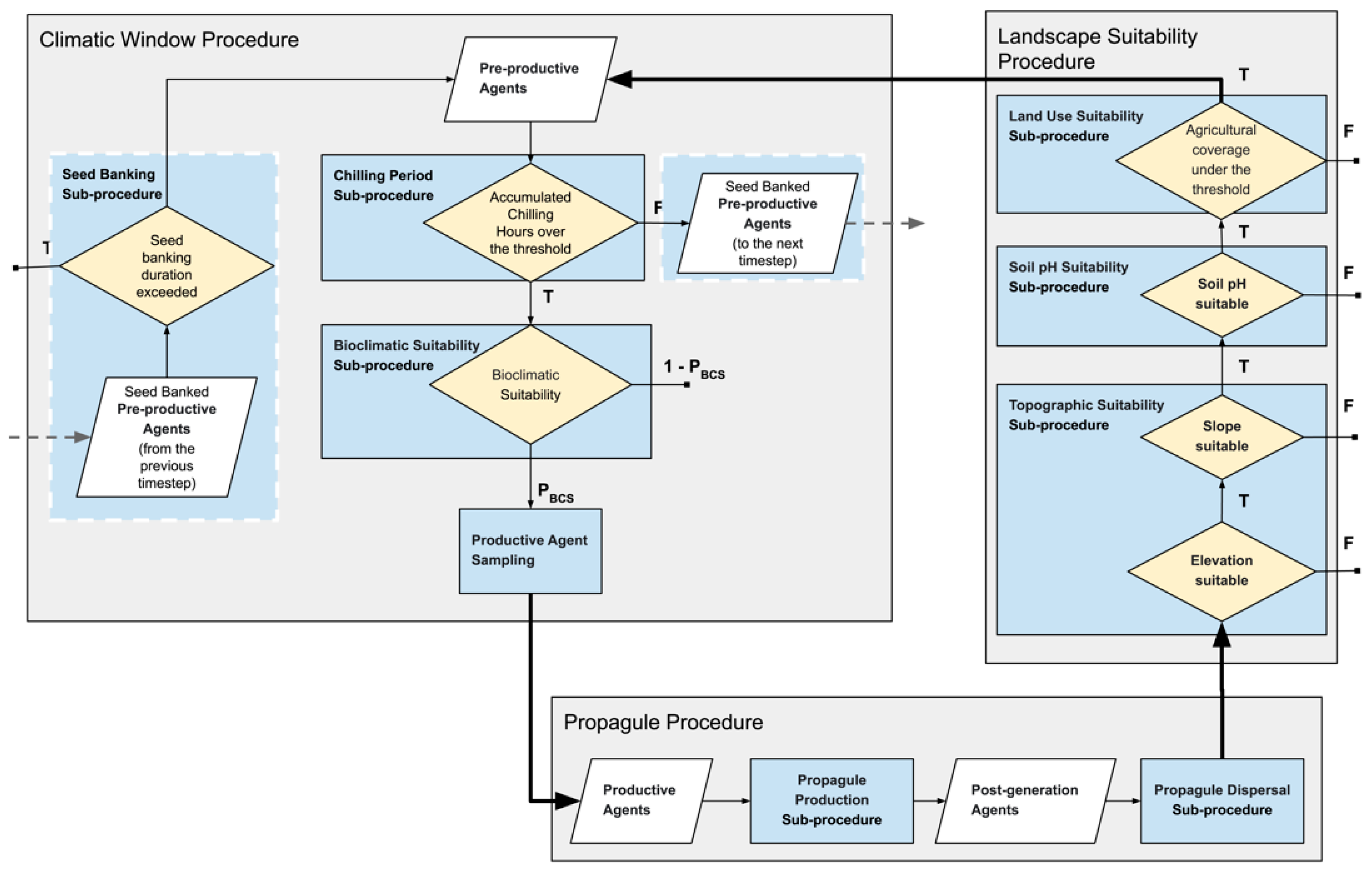
2.3.2. Agent Based Component

The ABC has three procedures, the Climatic Window Procedure, Propagule Procedure, and Landscape Suitability Procedure, in order of execution in a time step, and operates with three types of agents: productive agents, post-generation agents, and pre-productive agents. The workflow of the ABC is given in Figure 3. Productive agents represent the mature units with the capacity for seed production and correspond to the occurrence records. The initial productive agents are sampled from occurrence data with the assumption that all occurrence records were captured in their mature form. Post-generation agents are the generated and dispersed seeds produced by mature agents to germinate in the next time step. Pre-productive agents consist of ungerminated seeds and seed-banked pre-productive agents from previous time steps.

Climatic Window Procedure

The first phase of the ABC, in order of execution in a time step, is the Pre-productive Phase, which consists of: the chilling period, seed banking, bioclimatic suitability, and productive agent sampling sub-procedures. All environmental layers in this phase are yearly environmental layers.

I. glandulifera needs a chilling period in order to break dormancy and germinate [116], which occurs between February and March period [117]. Despite the required duration and temperature for proceeding of germination, reported as longer than 45 days at 4 °C [118] and one month at 5 °C [119], it is known that the parameters are highly variable depending on the seed properties and chilling period consistency. The chilling period was added to the framework with the following approach.

To determine a threshold based on the ACHs in the February–March period, 1234 occurrence records between 2005 to 2020 were assessed with the ACH layers of the respective years, with thresholds ranging between 600 to 1080 chilling hours. The threshold was determined as 720 chilling hours (30 days), since ~96% of the occurrences were observed to be recorded in the cells with ACH values over this threshold, which does not push the suitable zone unrealistically northward or southward. Occurrence records in the cells below the threshold may result from local habitat conditions that could not be captured by the coarse resolution of the ACH layers or other factors that are known to affect the germination process [120]. The chilling period sub-procedure uses the ACH layer of the corresponding year in accordance with the threshold value to assess the pre-productive agents. If the ACH value of the cell is above the threshold, the pre-productive agent proceeds to the Bioclimatic Suitability sub-procedure. If not, the agent is evaluated by seed the banking sub-procedure.

I. glandulifera is not known to form persistent and long-lasting seed banks [121], yet the seeds can survive longer than a year [86]. Accordingly, the seed banking duration variable, which determines in how many time steps a banked pre-productive agent is kept to be evaluated in the case of failure to pass the chilling period sub-procedure, was set as 1 year. The first seed banking is performed in the second time step, and the first evaluation of a seed-banked pre-productive agent occurs in the third time step, since the first time step starts with the propagule procedure.

The BCS layer of the corresponding time step, which the CC generates, is utilized in Bioclimatic Suitability sub-procedure. Although these layers can be thresholded to transform the probability/suitability data to presence/absence data with various methods [122], they were kept “as is” in the simulations. The cell values were used as probabilities to take advantage of the continuous and probabilistic nature of the projections to capture the gradients instead of sharp boundaries [123].

The pre-productive agents that can pass the sub-procedures of the Climatic Window Procedure are considered productive agents and correspond to the simulated occurrence records to be utilized by the CC. The Productive Agent Sampling sub-procedure involves a grid sampling operation with a 0.25° resolution occurrence map and is conducted in accordance with the sample per cell variable, which was set to 1 per cell for the simulations to identify the productive agents to proceed to the Propagule Procedure. While the grid sampling operation of the first step is performed with the initial occurrence records to reduce the inherent sampling bias in the occurrence data [45], which can lead to bias towards more intensively surveyed cells [124], it is responsible for scaling the population processed by the framework by determining the maximum number of productive agents on a cell in the occurrence map. In this regard, it must be noted that the population densities in the cells do not represent real populations due to the applied scaling.

Propagule Procedure

The second procedure of the ABC is the Propagule Procedure. It is mainly responsible for simulating the propagule pressure via its sub-procedures: Propagule Production and Propagule Dispersal. Propagule Procedure is the only procedure that does not use environmental layers due to its relatively generic structure.

The propagule Production sub-procedure performs the production of post-generation agents. The seed production of I. glandulifera is a well-documented subject both qualitatively and quantitatively [125,126,127]. However, determining the number of propagules produced by productive agents is not a straightforward task, as scaling is a common challenge of ABM applications. Thus, calibration simulations were conducted for different values of the propagule count to observe the model’s behavior. Consequently, 50 was determined as the propagule count, since further increments did not show drastic changes on the projected final invasive range and its latitudinal extremes, despite becoming computationally demanding with considerably longer runtimes.

Determination of dispersal direction and distance for the post-generation agents is performed in the Propagule Dispersal sub-procedure. For this implementation, an unsophisticated method was followed to simulate the short and mid-distance dispersal, and dispersal vectors were not explicitly distinguished. A random dispersal direction, drawn from the uniform distribution, was assigned to each post-generation agent; the dispersal distance for each post-generation agent was determined via a truncated negative exponential distribution. Maximum and mean dispersal distances were set as 38 km and 5 km, respectively [117], and the latter was used to determine the rate parameter of the negative exponential distribution.

Landscape Suitability Procedure

The third procedure of the ABC is the Landscape Suitability Procedure, which contains the Topographic Suitability, Soil pH Suitability, and Land Use Suitability sub-procedures. Since the successful transformation from post-generation agents to pre-productive agents is only possible if all the conditions are met, the execution order of the sub-procedures is not important.

The topographic Suitability sub-procedure evaluates the post-generation agents by using the elevation and slope layers. The elevational distribution of I. glandulifera differs between its native and invaded ranges. While it can grow on elevations exceeding 4000 m in its native range [55,117,128], it mostly occurs on lower elevations up to 600 m [59,125,126,127] in the invaded ranges. I. glandulifera mostly occurs on flat or slightly sloped terrains, up to 40° from horizontal, yet it is also known to be recorded on steeply sloping banks exceeding 40° [55]. The analysis conducted based on the Occ_Global and Occ_NA with elevation and slope data layers showed that 98.3% and 99.9% of the occurrences were under 1000 m elevation, respectively, and 99.9% of the occurrences were recorded on terrains with less than 20° median slope. Thus, the simulations were realized with a 1000 m maximum elevation and a 20° maximum slope limit. While the determined maximum slope limit was lower than that of the reports in the literature, the difference can be attributed to the coarse resolution of the slope data.

The Soil pH Suitability sub-procedure assesses the post-generation agents by using the soil pH data layer in accordance with the known soil pH tolerance of I. glandulifera, which is between 4.5 and 7.7 [129]. If the value of the cell is above or below the tolerance interval, the establishment is inhibited. Soil pH at 15 cm depth was selected, based on the shallow root length of I. glandulifera, which is about 10–20 cm [70,130].

The Land Use Suitability sub-procedure evaluates the post-generation agents by using the land use data layer of the corresponding time step and inhibits the establishment on the cells containing agricultural land over the threshold value. I. glandulifera is not known to infest agricultural lands, yet it is observed to occur on the field margins in its native range [55,128]. The same pattern has also been reported in its invaded range [70,131]. The analysis, conducted based on the Occ_Global and Occ_NA with 2020 land use data layers, showed that all the occurrence records were distributed over the cells with less than 80% agricultural coverage, except for one record. Consequently, 80% was determined as the maximum agricultural coverage limit for the simulations.

2.4. Initialization

All 50 simulations conducted for the study began with the grid sampling of the occurrence data from Occ_NA to determine the initial agents, which are the productive agents of the first time step. These agents were kept throughout the simulations to be processed by the ABC and CC, alongside the generated agents. Thus, the first time step did not include the first two sub-procedures of the Climatic Window Procedure and proceeded to the Propagule Procedure after the grid-sampling was performed by the Agent Sampling sub-procedure. Accordingly, every simulation was initialized with an equal number of invaded cells. However, due to the stochasticity, which resulted from sampling, the initial distribution of the agents was slightly different for each simulation. All defined variables and the assigned values used in the simulations are given in the Supplementary Materials, Table S2.

The initial extent of the simulations was determined based on the minimum bounding rectangle of the initial agent’s coordinates. Minimum and maximum longitude and latitudes were rounded with floor and ceiling functions. Then, a margin of 2° was added to obtain the initial extent. Following the first time step, the yearly extents were determined dynamically with the productive agent coordinates in the corresponding previous time step with the same method. The geographic extents were utilized for cropping the environmental layers and background point sampling.

2.5. Output

The yearly and 5-year inter-simulation agreement maps were constructed based on productive agents in the corresponding period to show the percentage of the simulations predicting the invasion of a particular cell. While the 5-year agreement maps were utilized for analysis to avoid the yearly fluctuation (Figure 4), the yearly agreement maps were presented as an animation, given in the Supplementary Materials (see Supplementary Animation).

The invaded cells or cell cumulations, which were initially present or formed during the simulations via merging and isolated from the others, are described with a loose term “focus” (plural foci) in the analysis. This naming is due to their role as the propagule source while expanding to the suitable areas. State, province, or geographic region and direction were used to signify the spatial context where they occur/were found (e.g., Ohio focus, Intermountain Region foci).

The foci, which the framework could not process throughout the simulations, were described as “irresponsive”. By the exclusion of the irresponsive California (3 cells), Newfoundland and Labrador (1 cell), and Northwest Territories (1 cell) foci, the analysis’ extent was determined as 140° W–60° W and 40° N–60° N. Due to reasons such as the somewhat independent invasion histories and the differences observed during the analysis, the extent was separated as east (60° W to 100° W) and west (100° W to 140° W) halves. All analyses were conducted based on moderate-agreement (>50%) cells.

Alongside the simulations, One-factor-at-a-time (OFAT) sensitivity analysis was also conducted. The OFAT sensitivity analysis method, which is performed by changing one parameter from a selected base parameter set (nominal set), while all other parameters are fixed to their nominal values, is used to determine the relationship between the varied parameter and output. OFAT provides an understanding of model mechanisms by demonstrating if the response is linear or nonlinear of the tipping points and whether there are tipping points where drastic responses occur with small parameter changes [132]. For the analysis, six parameters of ABC (Mean Dispersal Distance, Maximum Dispersal Distance, Propagule Production, Maximum Agricultural Coverage, Accumulated Chilling Hours, and Maximum Elevation) were used for five values with 10 simulations per case to detect the relationship between the variables and the invaded cell counts in the final 5-year period (Supplementary Table S3). The plots were constructed from the results, and the agreement maps for the final 5-year period of each case are given in the Supplementary Figures S1–S4.

3. Results

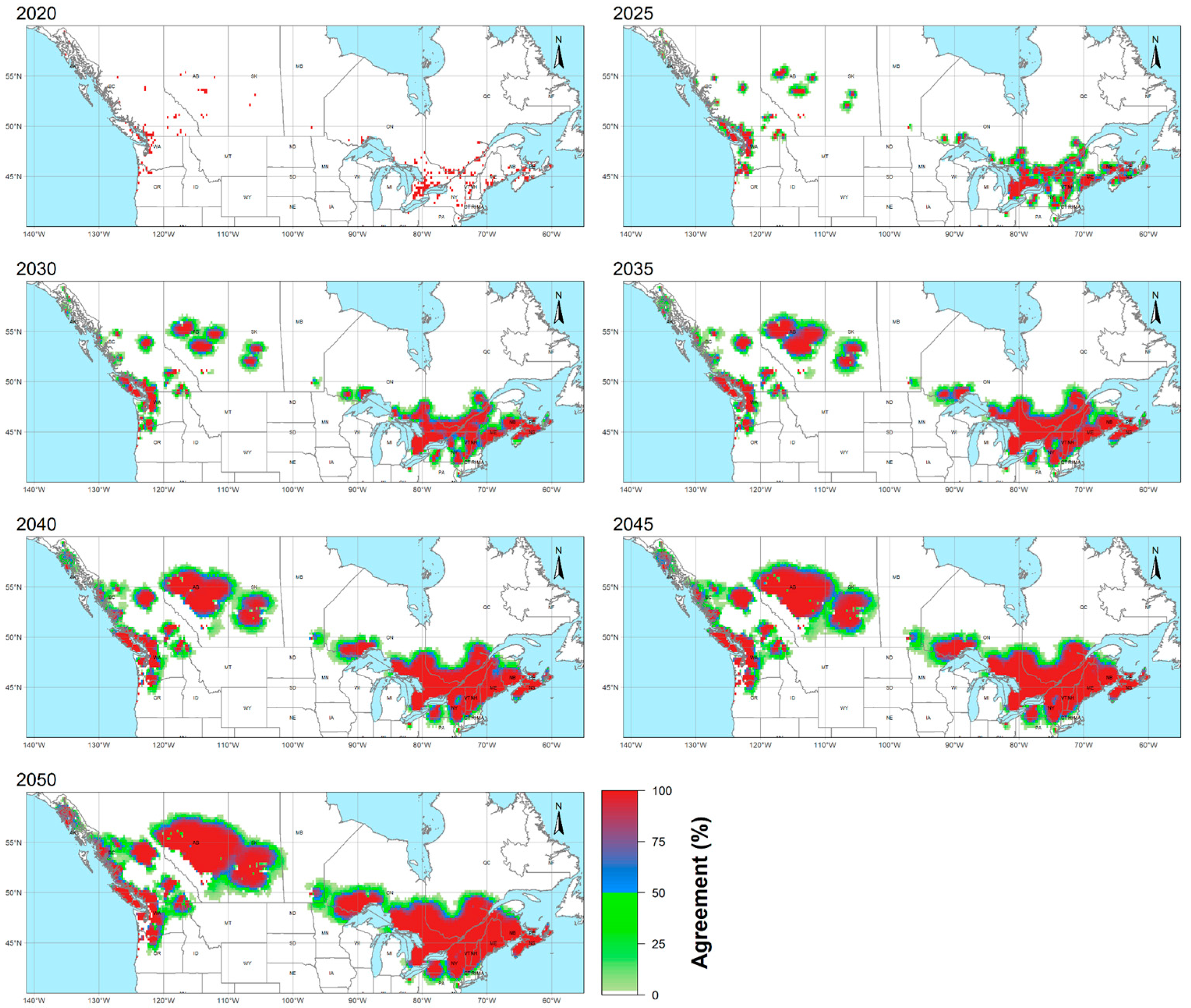
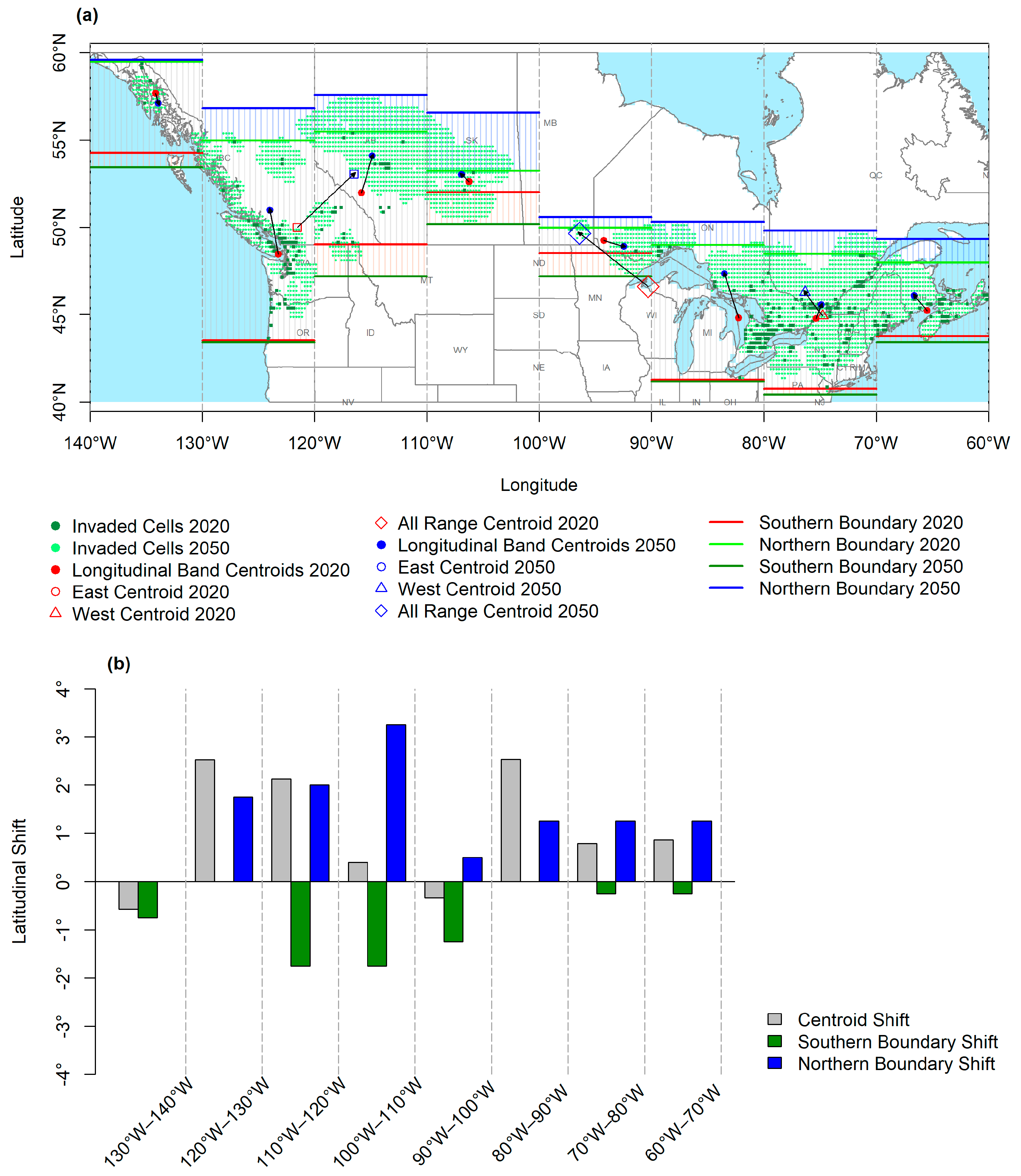
3.1. Geographic Overview

In the eastern half of the analysis’ extent, the projected invasive range was observed to cover provinces of the Maritimes (New Brunswick, Prince Edward Island, Nova Scotia), the northern states of the New England region (Vermont, New Hampshire, and Maine), the majority of New York, and the southern parts of Ontario and Quebec, with a high agreement. The southern boundary was observed to cross the northern parts of southern New England (Connecticut, Rhode Island, and Massachusetts), and Pennsylvania and was formed by the expansion of the neighboring areas. The Ohio and New Jersey foci, both located on the southern border of the invasive range in the eastern half, were observed to be stagnant and isolated from the rest of the high agreement zone of the invasive range. The northern boundary was formed by the northward expansion of the Quebec and Ontario foci, which were initially scattered on the shores of the Saint Lawrence River and Great Lakes, respectively.

The projected invasive range on the western half was primarily determined by the Pacific mountain ranges and was, consequently, more fragmented in comparison to the eastern half. The narrow range on the shores of British Columbia and Washington, which was limited by coastal ranges, was observed to continue to the north of Oregon, following the Cascades. No expansion was projected on the shores starting from the south of the Olympic Peninsula. In the Intermountain region of British Columbia, an expansion of several distinct foci, which were between the Rockies and coastal ranges, was observed. While the Fraser Plateau’s focus was the most prominent of these foci, the southernmost focus was slightly expanded to the north of Oregon, Idaho, and Montana. In Alaska, although the spread on the shores was limited, the Alexander Archipelago, especially the Admiralty, Baranof, and Chichagof Islands, was observed to be severely impacted. Arguably, the most striking projection obtained from the simulations was the formation that originated from the scattered foci of Alberta and Saskatchewan. The southern boundary was observed to be an arch crossing the north of Oregon, the southernmost focus of the Intermountain region, and south of Alberta–Saskatchewan. The northern boundary was determined primarily by Alaska and the north of Alberta–Saskatchewan.

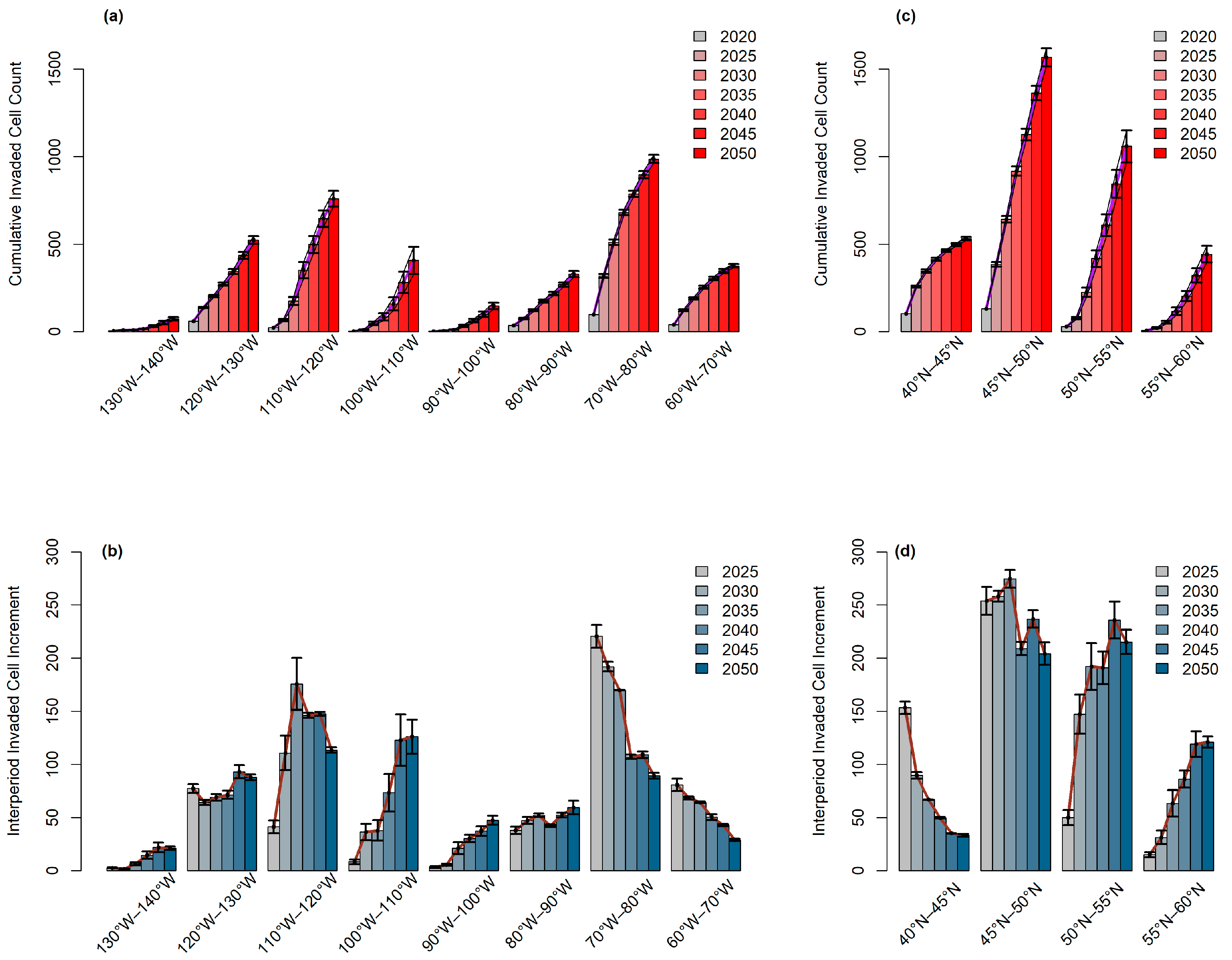
3.2. Longitudinal and Latitudinal Gradients

For detecting the changes in longitudinal and latitudinal gradients over the simulation period, results were also assessed regarding their Invaded Cell Count (ICC), the number of the invaded cells over each of the five-year periods (with the expectation of 2020, which was showing the initially invaded cell count), and Interperiod Invaded Cell Increment (IPI) difference between ICC values of consecutive periods, within longitudinal bands of 10° and latitudinal bands of 5°.

As seen in Figure 5a,b, 60° W–70° W and 70° W–80° W longitudinal bands, located in the easternmost of the invasive range and containing the East Coasts of Canada and the U.S.A., were the only bands to show an IPI decrease, which led to a prominent slowing trend in ICC throughout the simulation period. The 110° W–120° W band, which had the second highest final ICC, following the 60° W–70° W band, and primarily contained Alberta, was observed to show a slowing trend in ICC after mid-simulation in accordance with decreasing IPI. The 100° W–110° W band, which mainly contains Saskatchewan, did not show any significant slowing trend in ICC or IPI decrease. The linear ICC increase, due to IPI without a significant trend throughout the simulation period, was observed in the bands: 80° W–90° W, which contains the northern shores of the Great Lakes, and 120° W–130° W, which contains the west shores and the Intermountain region. In 90° W–100° W, containing Alaska, and 130° W–140° W, which contains Lake Superior, ICC was observed to increase after a lag period, albeit being relatively weak.

As for the latitudinal bands (see Figure 5c,d), the southernmost band, 40° N–45° N, demonstrated the most significant IPI decrease and ICC-slowing trend among all bands, including the longitudinal bands. IPI was also observed to have a negative trend for the 45° N–50° N band, which had the highest final ICC, despite being far less significant. For the 50° N–55° N and 55° N–60° N bands, primarily due to the increase in the Canadian Prairies, an accelerating ICC was observed, while IPI showed a slight decrease at the end of the period.

3.3. Latitudinal Shifts

The extent of the range shift was determined by evaluating the centroids and latitudinal extremes of the initial (2020) and final 5-year period (2050) distributions. Centroids were calculated with a rather unsophisticated method by calculating the mean values of latitudes and longitudes of invaded cells (see Figure 6a,b). Through the simulation period, the centroid of all invaded cells in the entire range was shifted 3.04° northward, while the shift for the eastern half was 1.35° and the west was 3.05°. Similarly, latitudes of the northern and southern extremes of each band were determined for the initial and final period distributions. Then, their respective differences were calculated to evaluate the shifts in the latitudinal boundaries. The mean shift of the northern boundary was observed to be 1.4° for the entire range, 1.06° for the eastern half, and 1.75° for the western half. The mean shift of the southern boundary was observed to be 0.75° for the entire range, 0.43° for the eastern half, and 1.06° for the western half.

When the latitudinal bands were examined individually, progression of the northern boundary, except the 140° W–130° W band, was observed to be common and pronounced compared to the progression of the southern boundary, which was primarily more pronounced for the bands initially containing foci on the higher latitudes. Individual centroids of the bands paralleled the progression of the northward boundaries, and all centroids were observed to shift northward, except the 140° W–130° W and 90° W–100° W bands.

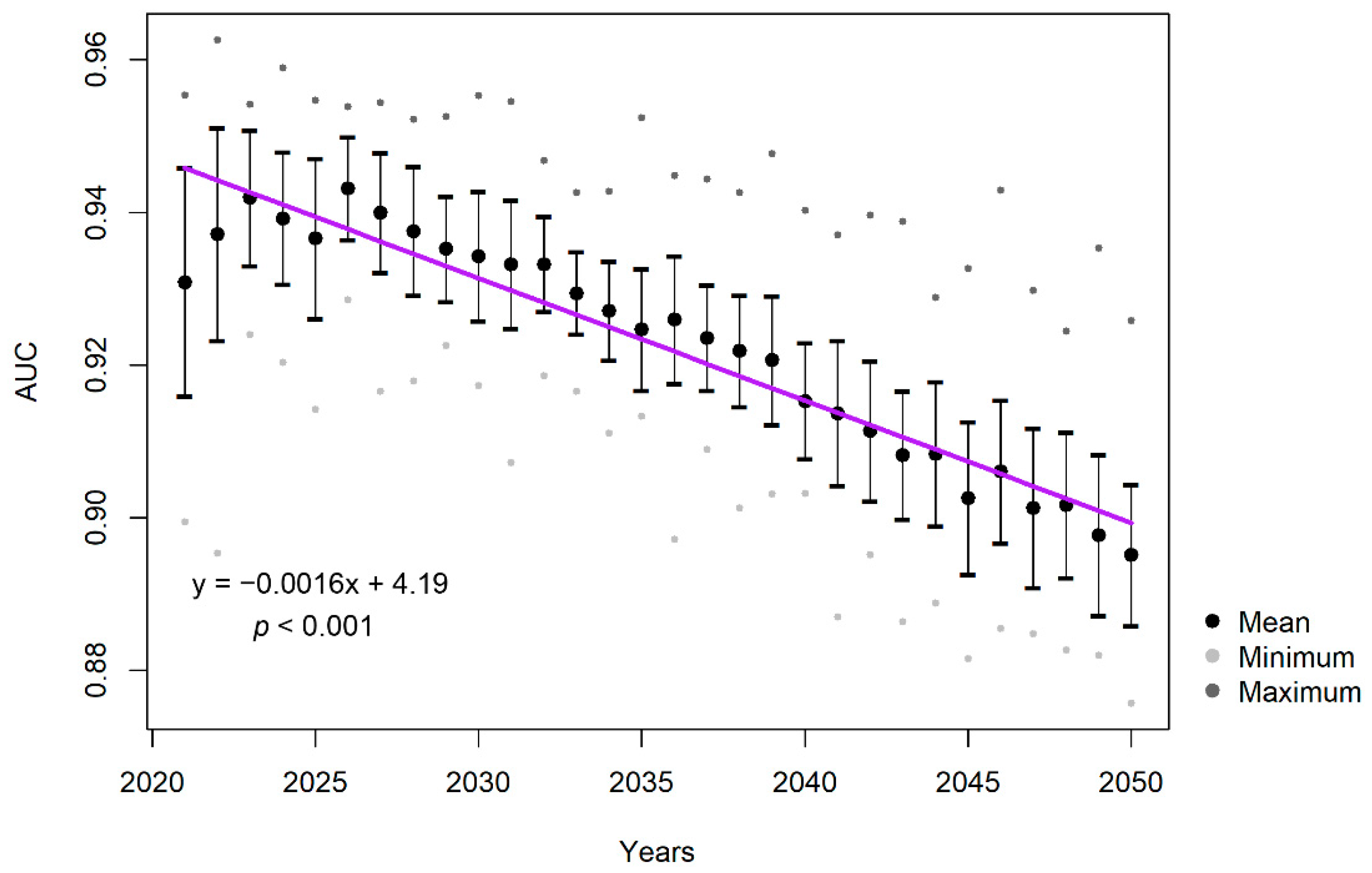
3.4. Predictive Performance of Correlative Component

The predictive performance of the CC, MaxEnt, was evaluated with AUC. AUC is one of the most extensively used statistics, measuring the ability of a model to discriminate the sites in which species are present from which the species are absent. AUC score ranges between 0 and 1, while 1 shows perfect discrimination and 0.5 implies the discrimination is not different from any random guess [133]. The mean AUC values of all simulations were observed to decrease through the simulation period with a significant trend (p < 0.01). However, considering the mean AUC for the first and last time step were 0.93 and 0.89, respectively, that decrease is acceptable for the time frame of the simulations (see Figure 7).

4. Discussion

The results from the simulations showed that I. glandulifera would increase its occurrence in the regions where it was currently present/reported in both the east and west parts, alongside an aggressive expansion in the interior regions in North America under the RCP 4.5 scenario. In particular, Alberta and Saskatchewan in the Canadian Prairies were projected to be a major invasive range, despite the currently limited I. glandulifera distribution. Many studies reported wide-scale poleward shift patterns due to climate change for a wide range of species (e.g., [134,135]). Invasive plants are not an exception (e.g., [136,137]), as this pattern was also projected for various invasive plants (e.g., [138,139,140,141]. Beerling [142] projected a northward invasive range expansion for I. glandulifera in Europe under climate change (solely the minimum winter temperature and growing degree days were used as predictors) [87], and these projections were supported by the increasing occurrence reports from higher latitudes in Europe in recent decades [73]. Following that, Tabak and von Wettberg [80] stated that the emergence of a similar pattern, i.e., a northward expansion, may also be expected for North America. Considering these, the northward expansion pattern shown by our results corresponded with the predictions in the reviewed literature.

The northern border of the projected invasive range was observed as roughly following the deciduous-boreal forest ecotone [143] in the East and the prairie-forest biome border [144] in the Alberta–Saskatchewan region in the West. The rapid warming in the boreal forests (approximately twice as fast as the global average [145]) and the projected northward shifts of warmer climate zones [146], e.g., the climatic shifts from prairies to the boreal forests [147,148], are expected to cause significant disturbances that can affect individual species and ecosystems and can lead to biome-level changes [149]. Partial or widespread removal of resident communities due to these disturbances [150], e.g., the formation of treefall gaps in ecotones, can increase the establishment and recruitment success of northward migrating temperate species [151]. Since I. glandulifera commonly occurs in ecotones [57], such conditions can increase invasion success. I. glandulifera seedlings are known to establish quickly in disturbed woodland sites [120], including woodland clearings and sparse woodlands [60] and, under some circumstances, to suppress woodland regeneration by facilitating the establishment of other species [58,152].

Drought stress, which has been more severe and frequent due to climate change, can affect I. glandulifera negatively by surpassing its physiological resistance strategies [153]. This finding is also supported by Beerling’s [142] predictions on the relationship between the southern boundary of I. glandulifera and summer droughts and the limited distribution of I. glandulifera in the south of Europe [56,73,87]. Consequently, the limited southward expansion of the projected invasive range and its geographical pattern is in accordance with the predicted increase in the drought severity and frequency with climate change for the USA and Canada [154,155,156,157].

I. glandulifera was recorded in Europe in the mountainous regions [66,88] in some cases at elevations exceeding 1000 m [53,158]. Additionally, recent studies reported an I. glandulifera spread in forests up to the timberline [60]. Moreover, elevational shifts of suitable habitats for tree populations due to climate change were also predicted [159]. Considering these facts, the projected expansion of invasive range in the mountainous regions in the west could be more severe by reaching elevations higher than the 1000 m elevation limit in our simulations. Another potential risk in recent decades is the increased impact of bark beetles with direct and indirect effects of climate change in the region [160], as the disturbances caused by bark beetle outbreaks facilitate a faster spread of I. glandulifera in forests [56,161].

The dispersal mechanism implemented in our framework simulated short and mid-distance dispersal, which led to the formation of patterns representing the spreading of invasive species with diffusion-like processes in short distances [162]. On the other hand, long-distance dispersal is typically connected to anthropogenic activities [163], and determining the potential consequences of these activities would constitute a limitation for the framework. I. glandulifera was observed to spread with forest machinery, river gravel, and topsoil, which is used for construction projects [56,164], ship ballasts [70], etc. Roads and railways are also known as its dispersal vectors [165,166]. However, trade is the most crucial factor in the spread of invasive species [167], and, as an ornamental, this is very true for I. glandulifera. The rise in the trading of invasive plants via e-commerce [168] in recent decades without effective biosecurity measures [169] constitutes a serious problem in many cases. It may serve the spread of invasive plants in an unpredictable and uncontrolled fashion. Given that the introduction of I. glandulifera outside of its native range was for horticultural purposes [117] and is still considered a popular ornamental with a remarkable economic value [170], anthropogenic impacts can drastically change the course of the invasion we projected.

To some extent, all SDMs are affected by the quality and completeness of, or biases in, the data [171,172]. Our study is not an exception and may be affected by such bias. Wallacean shortfalls [173], the incompleteness of species distribution data, and spatial and temporal biases are inherent in occurrence data [174,175]. Importantly, in the case of invasive species, lacking information such as whether the occurrences are recorded from an early stage of invasion [176] or whether they still reflect a stable relationship with the environment [177], constitute a source of potential problems in the context of equilibrium, which leads to bold yet unavoidable assumptions. Despite its crucial role as the largest initiative that provides occurrence data [178], GBIF is known to have pronounced biases [179]. As an example of the mentioned incompleteness, the reported presence of I. glandulifera in Anchorage, Alaska [82] was not included in the simulations, which may constitute a potential source of underestimation in the corresponding region, since it was absent in the data obtained from GBIF.

While our projections can be considered satisfactory as a preliminary attempt to provide an invasive range outline on a continental scale for North America, the framework, in its current state, does not include every factor that affects I. glandulifera invasion. The inclusion of these factors, e.g., biotic interactions, which can improve the accuracy of results, is planned for the further steps of our study. In consideration with the high competitive abilities of I. glandulifera, primarily due to allelopathic effects on co-occurring plant species, including dominant ones [180], soil fungal and bacterial communities [63], and even aquatic species in riparian habitats [181], are striking examples that emphasize the importance of such interactions on the invasion process. Although our approach is mainly centered around constraining the establishment and dispersal, in accordance with the modular structure, the framework can be extended to simulate the processes facilitating establishment. Additionally, implementing a more sophisticated dispersal mechanism to simulate the dispersal vectors (such as animals [57,117]) explicitly, especially the inclusion of river networks alongside higher resolution environmental data in finer geographic scales, can be highly beneficial to make more accurate projections. It is also worth mentioning that the approach we follow can be adapted to be utilized for other species after the generalization of the design, which we plan for the upcoming steps of the study, regardless of the current ad hoc structure of the framework.

Eradication of I. glandulifera is costly [182] and even futile after its spread in interconnected lowland watercourses [52]. Eradication efforts can lead to an invasional meltdown, as the sites after the removal are much more prone to be invaded by other invasive plants [62]. Thus, habitat restoration is a must, along with removal [58]. Chemical control is an available [75] but a not yet viable choice for riparian habitats [183]. Mechanical control is expensive and laborious [184]. The effects of fungal pathogens on biological control vary between the populations [185]. I. glandulifera, as Bieberich suggests [186], is a back-seat driver facilitated by previous ecosystem changes and also a driver of further changes. Thus, habitat stability is more important than the habitat type to explain its impacts [58]. In this respect, management and conservation strategies should be evaluated for local conditions. Preventive measures and monitoring are needed to keep the current distribution under control and prevent further spread to habitats that are already under the impact of global environmental change.

References

1. Vitousek, P.M. Beyond global warming: Ecology and global change. Ecology 1994, 75, 1861–1876. [Google Scholar] [CrossRef]
2. Mainka, S.A.; Howard, G.W. Climate. change and invasive species: Double jeopardy. Integr. Zool. 2010, 5, 102–111. [Google Scholar] [CrossRef] [PubMed]
3. Masters, G.; Norgrove, L. Climate Change and Invasive Alien Species; CABI Working Paper 1; CABI: Wallingford, UK, 2010; p. 30. [Google Scholar]
4. Vitousek, P.M. Global environmental change: An introduction. Annu. Rev. Ecol. Syst. 1992, 23, 1–14. [Google Scholar] [CrossRef]
5. Novacek, M.J.; Cleland, E.E. The current biodiversity extinction event: Scenarios for mitigation and recovery. Proc. Natl. Acad. Sci. USA 2001, 98, 5466–5470. [Google Scholar] [CrossRef] [Green Version]
6. Evans, E.A. Economic dimensions of invasive species. Choices 2003, 18, 5–9. [Google Scholar] [CrossRef]
7. Ziska, L.H.; Blumenthal, D.M.; Runion, G.B.; Hunt, E.R.; Diaz-Soltero, H. Invasive species and climate change: An agronomic perspective. Clim. Chang. 2011, 105, 13–42. [Google Scholar] [CrossRef]
8. IUCN. Invasive Alien Species and Climate Change. 2021. Available online: https://www.iucn.org/resources/issues-briefs/invasive-alien-species-and-climate-change (accessed on 7 December 2021).
9. Ehrenfeld, J.G. Ecosystem consequences of biological invasions. Annual review of ecology, evolution, and systematics. Annu. Rev. 2010, 41, 59–80. [Google Scholar] [CrossRef] [Green Version]
10. Rahel, F.J. Homogenization of freshwater faunas. Annu. Rev. Ecol. Syst. 2002, 33, 291–315. [Google Scholar] [CrossRef] [Green Version]
11. Olden, J.D.; Lockwood, J.L.; Parr, C.L. Biological invasions and the homogenization of faunas and floras. Conserv. Biogeogr. 2011, 9, 224–244. [Google Scholar] [CrossRef]
12. Brooks, M.L.; Pyke, D.A. Invasive plants and fire in the deserts of North America. In Proceedings of the Invasive Species Workshop: The Role of Fire in the Control and Spread of Invasive Species. Fire Conference 2000: The First National Congress on Fire Ecology, Prevention and Management, San Diego, CA, USA, 27 November–1 December 2000; Miscellaneous Publication No. 11. Galley, K.E.M., Wilson, T.P., Eds.; Tall Timbers Research Station: Tallahassee, FL, USA, 2001; pp. 1–14. [Google Scholar]
13. Brooks, M.L.; D’antonio, C.M.; Richardson, D.M.; Grace, J.B.; Keeley, J.E.; DiTomaso, J.M.; Hobbs, R.J.; Pellant, M.; Pyke, D. Effects of invasive alien plants on fire regimes. BioScience 2004, 54, 677–688. [Google Scholar] [CrossRef] [Green Version]
14. Keeley, J.E. Fire and invasive species in Mediterranean-climate ecosystems of California. In Proceedings of the Invasive Species Workshop: The Role of Fire in the Control and Spread of Invasive Species. Fire Conference 2000: The First National Congress on Fire Ecology, Prevention and Management, San Diego, CA, USA, 27 November–1 December 2000; Miscellaneous publication: 11. Galley, K.E.M., Wilson, T.P., Eds.; Tall Timbers Research Station: Tallahassee, FL, USA, 2001; pp. 81–94. [Google Scholar]
15. Simberloff, D. How common are invasion-induced ecosystem impacts? Biol. Invasions 2011, 13, 1255–1268. [Google Scholar] [CrossRef]
16. Crystal-Ornelas, R.; Hudgins, E.J.; Cuthbert, R.N.; Haubrock, P.J.; Fantle-Lepczyk, J.; Angulo, E.; Kramer, A.M.; Ballesteros-Mejia, L.; Leroy, B.; Leung, B.; et al. Economic costs of biological invasions within North America. NeoBiota 2021, 67, 485. [Google Scholar] [CrossRef]
17. Diagne, C.; Leroy, B.; Vaissière, A.C.; Gozlan, R.E.; Roiz, D.; Jarić, I.; Salles, J.M.; Bradshaw, C.J.; Courchamp, F. High and rising economic costs of biological invasions worldwide. Nature 2021, 592, 571–576. [Google Scholar] [CrossRef]
18. Pejchar, L.; Mooney, H.A. Invasive species, ecosystem services and human well-being. Trends Ecol. Evol. 2009, 24, 497–504. [Google Scholar] [CrossRef] [PubMed]
19. Cook, D.C.; Fraser, R.W.; Paini, D.R.; Warden, A.C.; Lonsdale, W.M.; De Barro, P.J. Biosecurity and yield improvement technologies are strategic complements in the fight against food insecurity. PLoS ONE 2011, 6, e26084. [Google Scholar] [CrossRef] [PubMed] [Green Version]
20. Seebens, H.; Blackburn, T.M.; Dyer, E.E.; Genovesi, P.; Hulme, P.E.; Jeschke, J.M.; Pagad, S.; Pyšek, P.; Winter, M.; Arianoutsou, M.; et al. No saturation in the accumulation of alien species worldwide. Nat. Commun. 2017, 8, 14435. [Google Scholar] [CrossRef] [PubMed]
21. Mack, R.N.; Simberloff, D.; Mark Lonsdale, W.; Evans, H.; Clout, M.; Bazzaz, F.A. Biotic invasions: Causes, epidemiology, global consequences, and control. Ecol. Appl. 2000, 10, 689–710. [Google Scholar] [CrossRef]
22. Thomas, S.M.; Moloney, K.A. Combining the effects of surrounding land-use and propagule pressure to predict the distribution of an invasive plant. Biol. Invasions 2015, 17, 477–495. [Google Scholar] [CrossRef]
23. Petitpierre, B.; Kueffer, C.; Broennimann, O.; Randin, C.; Daehler, C.; Guisan, A. Climatic niche shifts are rare among terrestrial plant invaders. Science 2012, 335, 1344–1348. [Google Scholar] [CrossRef] [PubMed] [Green Version]
24. Thuiller, W. Climate change and the ecologist. Nature 2007, 448, 550–552. [Google Scholar] [CrossRef]
25. Ladle, R.J.; Malhado, A.C.; Correia, R.A.; dos Santos, J.G.; Santos, A.M. Research trends in biogeography. J. Biogeogr. 2015, 42, 2270–2276. [Google Scholar] [CrossRef]
26. Soberón, J.; Peterson, T. Biodiversity informatics: Managing and applying primary biodiversity data. Philos. Trans. R. Soc. Lond. Ser. B Biol. Sci. 2004, 359, 689–698. [Google Scholar] [CrossRef] [PubMed]
27. Blair, G.S.; Henrys, P.; Leeson, A.; Watkins, J.; Eastoe, E.; Jarvis, S.; Young, P.J. Data science of the natural environment: A research roadmap. Front. Environ. Sci. 2019, 7, 121. [Google Scholar] [CrossRef] [Green Version]
28. Jiménez-Valverde, A.; Peterson, A.T.; Soberón, J.; Overton, J.M.; Aragón, P.; Lobo, J.M. Use of niche models in invasive species risk assessments. Biol. Invasions 2011, 13, 2785–2797. [Google Scholar] [CrossRef]
29. Araújo, M.B.; Anderson, R.P.; Márcia Barbosa, A.; Beale, C.M.; Dormann, C.F.; Early, R.; Garcia, R.A.; Guisan, A.; Maiorano, L.; Naimi, B.; et al. Standards for distribution models in biodiversity assessments. Sci. Adv. 2019, 5, eaat4858. [Google Scholar] [CrossRef] [Green Version]
30. Sofaer, H.R.; Jarnevich, C.S.; Pearse, I.S.; Smyth, R.L.; Auer, S.; Cook, G.L.; Edwards, T.C., Jr.; Guala, G.F.; Howard, T.G.; Morisette, J.T.; et al. Development and delivery of species distribution models to inform decision-making. BioScience 2019, 69, 544–557. [Google Scholar] [CrossRef]
31. Elith, J.; Leathwick, J.R. Species distribution models: Ecological explanation and prediction across space and time. Annu. Rev. Ecol. Evol. Syst. 2009, 40, 677–697. [Google Scholar] [CrossRef]
32. Beale, C.M.; Lennon, J.J. Incorporating uncertainty in predictive species distribution modelling. Philos. Trans. R. Soc. B Biol. Sci. 2012, 367, 247–258. [Google Scholar] [CrossRef] [PubMed]
33. Werkowska, W.; Márquez, A.L.; Real, R.; Acevedo, P. A practical overview of transferability in species distribution modeling. Environ. Rev. 2017, 25, 127–133. [Google Scholar] [CrossRef]
34. Bradley, B.A.; Wilcove, D.S.; Oppenheimer, M. Climate change increases risk of plant invasion in the Eastern United States. Biol. Invasions 2010, 12, 1855–1872. [Google Scholar] [CrossRef]
35. Padalia, H.; Srivastava, V.; Kushwaha, S.P.S. Modeling potential invasion range of alien invasive species, Hyptis suaveolens (L.) Poit. in India: Comparison of MaxEnt and GARP. Ecol. Inform. 2014, 22, 36–43. [Google Scholar] [CrossRef]
36. Mainali, K.P.; Warren, D.L.; Dhileepan, K.; McConnachie, A.; Strathie, L.; Hassan, G.; Karki, D.; Shrestha, B.B.; Parmesan, C. Projecting future expansion of invasive species: Comparing and improving methodologies for species distribution modeling. Glob. Chang. Biol. 2015, 21, 4464–4480. [Google Scholar] [CrossRef] [Green Version]
37. West, A.M.; Kumar, S.; Brown, C.S.; Stohlgren, T.J.; Bromberg, J. Field validation of an invasive species Maxent model. Ecol. Inform. 2016, 36, 126–134. [Google Scholar] [CrossRef] [Green Version]
38. Jeschke, J.M.; Strayer, D.L. Usefulness of bioclimatic models for studying climate change and invasive species. Ann. N. Y. Acad. Sci. 2008, 1134, 1–24. [Google Scholar] [CrossRef]
39. Guillaumot, C.; Belmaker, J.; Buba, Y.; Fourcy, D.; Dubois, P.; Danis, B.; Le Moan, E.; Saucède, T. Classic or hybrid? The performance of next generation ecological models to study the response of Southern Ocean species to changing environmental conditions. Divers. Distrib. 2022, 28, 2286–2302. [Google Scholar] [CrossRef]
40. Parrott, L. Hybrid modelling of complex ecological systems for decision support: Recent successes and future perspectives. Ecol. Inform. 2011, 6, 44–49. [Google Scholar] [CrossRef]
41. 41] Gallien, L.; Münkemüller, T.; Albert, C.H.; Boulangeat, I.; Thuiller, W. Predicting potential distributions of invasive species: Where to go from here? Divers. Distrib. 2010, 16, 331–342. [Google Scholar] [CrossRef]
42. Srivastava, V.; Lafond, V.; Griess, V.C. Species distribution models (SDM): Applications, benefits and challenges in invasive species management. CAB Rev. 2019, 14, 1–13. [Google Scholar] [CrossRef]
43. Engler, R.; Guisan, A. MigClim: Predicting plant distribution and dispersal in a changing climate. Divers. Distrib. 2009, 15, 590–601. [Google Scholar] [CrossRef]
44. Smolik, M.; Dullinger, S.; Essl, F.; Kleinbauer, I.; Leitner, M.; Peterseil, J.; Stadler, L.-M.; Vogl, G. Integrating species distribution models and interacting particle systems to predict the spread of an invasive alien plant. J. Biogeogr. 2010, 37, 411–422. [Google Scholar] [CrossRef]
45. Williams, R.J.; Dunn, A.M.; Mendes da Costa, L.; Hassall, C. Climate and habitat configuration limit range expansion and patterns of dispersal in a non-native lizard. Ecol. Evol. 2021, 11, 3332–3346. [Google Scholar] [CrossRef] [PubMed]
46. Meier, E.S.; Dullinger, S.; Zimmermann, N.E.; Baumgartner, D.; Gattringer, A.; Hülber, K. Space matters when defining effective management for invasive plants. Divers. Distrib. 2014, 20, 1029–1043. [Google Scholar] [CrossRef]
47. DeAngelis, D.L.; Grimm, V. Individual-based models in ecology after four decades. F1000Prime Rep. 2014, 6, 39. [Google Scholar] [CrossRef] [PubMed] [Green Version]
48. Buckley, Y.M.; Briese, D.T.; Rees, M. Demography and management of the invasive plant species Hypericum perforatum. II. Construction and use of an individual-based model to predict population dynamics and the effects of management strategies. J. Appl. Ecol. 2003, 40, 494–507. [Google Scholar] [CrossRef]
49. Rebaudo, F.; Crespo-Pérez, V.; Silvain, J.F.; Dangles, O. Agent-based modeling of human-induced spread of invasive species in agricultural landscapes: Insights from the potato moth in Ecuador. J. Artif. Soc. Soc. Simul. 2011, 14, 7. [Google Scholar] [CrossRef]
50. Fraser, E.J.; Lambin, X.; Travis, J.M.; Harrington, L.A.; Palmer, S.C.; Bocedi, G.; Macdonald, D.W. Range expansion of an invasive species through a heterogeneous landscape–the case of American mink in Scotland. Divers. Distrib. 2015, 21, 888–900. [Google Scholar] [CrossRef] [Green Version]
51. Aurambout, J.P.; Endress, A.G. A model to simulate the spread and management cost of kudzu (Pueraria montana var. lobata) at landscape scale. Ecol. Inform. 2018, 43, 146–156. [Google Scholar] [CrossRef]
52. Pattison, Z.; Vallejo-Marín, M.; Willby, N. Riverbanks as battlegrounds: Why does the abundance of native and invasive plants vary? Ecosystems 2019, 22, 578–586. [Google Scholar] [CrossRef] [Green Version]
53. Pyšek, P.; Prach, K. Invasion dynamics of Impatiens glandulifera—A century of spreading reconstructed. Biol. Conserv. 1995, 74, 41–48. [Google Scholar] [CrossRef]
54. Millane, M.; Caffrey, J.M. Risk Assessment of Impatiens Glandulifera. Inland Fisheries Ireland; National Biodiversity Centre: Dublin, Ireland, 2014; 29p. Available online: http://nonnativespecies.ie/wp–content/uploads/2014/03/Impatiens-glandulifera-Himalayan-balsam1.pdf (accessed on 7 August 2022).
55. Drescher, A.; Prots, B. Warum breitet sich das Drüsen-Springkraut (Impatiens glandulifera Royle) in den Alpen aus? Wulfenia 2000, 7, 5–26. [Google Scholar]
56. Čuda, J.; Skálová, H.; Pyšek, P. Spread of Impatiens glandulifera from riparian habitats to forests and its associated impacts: Insights from a new invasion. Weed Res. 2020, 60, 8–15. [Google Scholar] [CrossRef]
57. Čuda, J.; Rumlerová, Z.; Brůna, J.; Skálová, H.; Pyšek, P. Floods affect the abundance of invasive Impatiens glandulifera and its spread from river corridors. Divers. Distrib. 2017, 23, 342–354. [Google Scholar] [CrossRef] [Green Version]
58. Coakley, S.; Petti, C. Impacts of the invasive Impatiens glandulifera: Lessons learned from one of Europe’s top invasive species. Biology 2021, 10, 619. [Google Scholar] [CrossRef]
59. Hejda, M.; Pyšek, P. What is the impact of Impatiens glandulifera on species diversity of invaded riparian vegetation? Biol. Conserv. 2006, 132, 143–152. [Google Scholar] [CrossRef]
60. Čuda, J.; Vítková, M.; Albrechtová, M.; Guo, W.Y.; Barney, J.N.; Pyšek, P. Invasive herb Impatiens glandulifera has minimal impact on multiple components of temperate forest ecosystem function. Biol. Invasions 2017, 19, 3051–3066. [Google Scholar] [CrossRef]
61. Diekmann, M.; Effertz, H.; Baranowski, M.; Dupré, C. Weak effects on plant diversity of two invasive Impatiens species. Plant Ecol. 2016, 217, 1503–1514. [Google Scholar] [CrossRef]
62. Hulme, P.E.; Bremner, E.T. Assessing the impact of Impatiens glandulifera on riparian habitats: Partitioning diversity components following species removal. J. Appl. Ecol. 2006, 43, 43–50. [Google Scholar] [CrossRef]
63. Gaggini, L.; Rusterholz, H.P.; Baur, B. The invasive plant Impatiens glandulifera affects soil fungal diversity and the bacterial community in forests. Appl. Soil Ecol. 2018, 124, 335–343. [Google Scholar] [CrossRef]
64. Hejda, M.; Pyšek, P.; Jarošík, V. Impact of invasive plants on the species richness, diversity and composition of invaded communities. J. Ecol. 2009, 97, 393–403. [Google Scholar] [CrossRef]
65. Jamin, J.; Diehl, D.; Meyer, M.; David, J.; Schaumann, G.E.; Buchmann, C. Physico-Chemical Soil Properties Affected by Invasive Plants in Southwest Germany (Rhineland-Palatinate)—A Case Study. Soil Syst. 2022, 6, 93. [Google Scholar] [CrossRef]
66. Kiełtyk, P.; Delimat, A. Impact of the alien plant Impatiens glandulifera on species diversity of invaded vegetation in the northern foothills of the Tatra Mountains, Central Europe. Plant Ecol. 2019, 220, 1–12. [Google Scholar] [CrossRef] [Green Version]
67. Dassonville, N.; Vanderhoeven, S.; Vanparys, V.; Hayez, M.; Gruber, W.; Meerts, P. Impacts of alien invasive plants on soil nutrients are correlated with initial site conditions in NW Europe. Oecologia 2008, 157, 131–140. [Google Scholar] [CrossRef]
68. Rusterholz, H.P.; Küng, J.; Baur, B. Experimental evidence for a delayed response of the above-ground vegetation and the seed bank to the invasion of an annual exotic plant in deciduous forests. Basic Appl. Ecol. 2017, 20, 19–30. [Google Scholar] [CrossRef]
69. Greenwood, P.; Kuhn, N.J. Does the invasive plant, Impatiens glandulifera, promote soil erosion along the riparian zone? An investigation on a small watercourse in northwest Switzerland. J. Soils Sediments 2014, 14, 637–650. [Google Scholar] [CrossRef]
70. Clements, D.R.; Feenstra, K.R.; Jones, K.; Staniforth, R. The biology of invasive alien plants in Canada. 9. Impatiens glandulifera Royle. Can. J. Plant Sci. 2008, 88, 403–417. [Google Scholar] [CrossRef] [Green Version]
71. Burkhart, K.; Nentwig, W. Control of Impatiens glandulifera (Balsaminaceae) by antagonists in its invaded range. Invasive Plant Sci. Manag. 2008, 1, 352–358. [Google Scholar] [CrossRef]
72. Tanner, R.A.; Jin, L.; Shaw, R.; Murphy, S.T.; Gange, A.C. An Ecological Assessment of Impatiens glandulifera in its Introduced and Native Range and the Potential for its Classical Biological Control. Ph.D. Thesis, Royal Holloway, University of London, London, UK, 2012. [Google Scholar] [CrossRef]
73. Global Biodiversity Information Facility (GBIF). Impatiens Glandulifera Royle. 2022. Available online: https://www.gbif.org/species/2891770 (accessed on 12 August 2022).
74. GLANSIS. Impatiens Glandulifera Royle. Available online: https://nas.er.usgs.gov/queries/GreatLakes/FactSheet.aspx?Species_ID=2695 (accessed on 10 August 2022).
75. CABI Digital Library. Impatiens Glandulifera (Himalayan Balsam). Available online: https://www.cabidigitallibrary.org/doi/10.1079/cabicompendium.28766 (accessed on 12 August 2022).
76. USDA. Impatiens Glandulifera Royle. Available online: https://plants.usda.gov/home/plantProfile?symbol=IMGL (accessed on 13 August 2022).
77. Invasive Species Centre. Himalayan Balsam (Impatiens Glandulifera). Available online: https://www.invasivespeciescentre.ca/invasive-species/meet-the-species/invasive-plants/himalayan-balsam/ (accessed on 12 August 2022).
78. IPANE. Impatiens Glandulifera. Available online: https://www.invasive.org/weedcd/pdfs/ipane/Impatiensglandulifera.pdf (accessed on 14 August 2022).
79. Toney, J.C.; Rice, P.M.; Forecella, F. Exotic plant records in the northwest United States 1950–1996: An ecological assessment. Northwest Sci. 1998, 72, 198–213. [Google Scholar] [CrossRef]
80. Tabak, N.M.; von Wettberg, E. Native and introduced jewelweeds of the Northeast. Northeast. Nat. 2008, 15, 159–176. [Google Scholar] [CrossRef]
81. Mills, E.L.; Leach, J.H.; Carlton, J.T.; Secor, C.L. Exotic species in the Great Lakes: A history of biotic crises and anthropogenic introductions. J. Great Lakes Res. 1993, 19, 1–54. [Google Scholar] [CrossRef]
82. Alaska Center for Conservation Science (ACCS). Available online: https://accs.uaa.alaska.edu/invasive-species/non-native-plant-species-list/ (accessed on 11 December 2022).
83. Adamowski, W. Status of Impatiens Genus in Mexico—Research Proposal. 2019. Available online: https://www.researchgate.net/publication/331210846_Status_of_Impatiens_genus_in_Mexico_-_research_proposal (accessed on 1 October 2022).
84. Kurtto, A. Impatiens glandulifera (Balsaminaceae) as an ornamental and escape in Finland, with notes on the other Nordic countries. Acta Univ. Ups. Symb. Bot. Ups. 1996, 31, 221–228. [Google Scholar]
85. Prots, B.; Drescher, A. Role of dispersal agents for the spread of Impatiens glandulifera in Transcarpathia. J. Biol. Syst. 2010, 2, 42–46. [Google Scholar]
86. Perrins, J.; Fitter, A.; Williamson, M. Population biology and rates of invasion of three introduced Impatiens species in the British Isles. J. Biogeogr. 1993, 20, 33–44. [Google Scholar] [CrossRef]
87. Helsen, K.; Diekmann, M.; Decocq, G.; De Pauw, K.; Govaert, S.; Graae, B.J.; Hagenblad, J.; Liira, J.; Orczewska, A.; Sanczuk, P.; et al. Biological flora of Central Europe: Impatiens glandulifera Royle. Perspect. Plant Ecol. Evol. Syst. 2021, 50, 125609. [Google Scholar] [CrossRef]
88. Vorstenbosch, T.; Essl, F.; Lenzner, B. An uphill battle? The elevational distribution of alien plant species along rivers and roads in the Austrian Alps. NeoBiota 2020, 63, 1–24. [Google Scholar] [CrossRef]
89. Carlton, J.T. Pattern, process, and prediction in marine invasion ecology. Biol. Conserv. 1996, 78, 97–106. [Google Scholar] [CrossRef]
90. Johnstone, I.M. Plant invasion windows: A time-based classification of invasion potential. Biol. Rev. 1986, 61, 369–394. [Google Scholar] [CrossRef]
91. Crawley, M.J. Chance and timing in biological invasions. In Biological Invasions: A Global Perspective; Wiley: New York, NY, USA, 1989; pp. 407–424. [Google Scholar]
92. Ehrlich, P. Attributes of invaders and the invading processes vertebrates. In Biological Invasions: A Global Perspective; Wiley: New York, NY, USA, 1989; pp. 315–328. [Google Scholar]
93. Kramer-Schadt, S.; Niedballa, J.; Pilgrim, J.D.; Schröder, B.; Lindenborn, J.; Reinfelder, V.; Stillfried, M.; Heckmann, I.; Scharf, A.K.; Augeri, D.M.; et al. The importance of correcting for sampling bias in MaxEnt species distribution models. Divers. Distrib. 2013, 19, 1366–1379. [Google Scholar] [CrossRef]
94. R Core Team. R: A Language and Environment for Statistical Computing; R Foundation for Statistical Computing: Vienna, Austria, 2022. [Google Scholar]
95. RStudio Team. RStudio: Integrated Development for R; RStudio, PBC: Boston, MA, USA, 2022; Available online: http://www.rstudio.com/ (accessed on 22 April 2018).
96. Phillips, S.J.; Dudík, M.; Schapire, R.E. Maxent Software for Modeling Species Niches and Distributions (Version 3.4.1). 2022. Available online: http://biodiversityinformatics.amnh.org/open_source/maxent/ (accessed on 3 December 2018).
97. Hijmans, R.J.; Phillips, S.; Leathwick, J.; Elith, J. Dismo: Species Distribution Modeling. R-Package Version 1.3-3. 2020. Available online: https://CRAN.R-project.org/package=dismo (accessed on 5 December 2018).
98. GBIF.org. GBIF Occurrence Download. 2022. Available online: https://www.gbif.org/occurrence/download/0265702-210914110416597 (accessed on 5 May 2022).
99. Hersbach, H.; Bell, B.; Berrisford, P.; Biavati, G.; Horányi, A.; Muñoz Sabater, J.; Nicolas, J.; Peubey, C.; Radu, R.; Rozum, I.; et al. ERA5 Hourly Data on Single Levels from 1940 to Present. Copernicus Climate Change Service (C3S) Climate Data Store (CDS). 2021. Available online: https://cds.climate.copernicus.eu/cdsapp#!/dataset/reanalysis-era5-single-levels?tab=overview (accessed on 10 June 2021).
100. ERA5-Land Monthly Averaged Data from 1950 to Present. Available online: https://cds.climate.copernicus.eu/cdsapp#!/dataset/reanalysis-era5-land-monthly-means?tab=overview (accessed on 15 June 2021).
101. Watanabe, M.; Suzuki, T.; O’ishi, R.; Komuro, Y.; Watanabe, S.; Emori, S.; Takemura, T.; Chikira, M.; Ogura, T.; Sekiguchi, M.; et al. Improved climate simulation by MIROC5: Mean states, variability, and climate sensitivity. J. Clim. 2010, 23, 6312–6335. [Google Scholar] [CrossRef]
102. Thrasher, B.; Maurer, E.P.; McKellar, C.; Duffy, P.B. Bias correcting climate model simulated daily temperature extremes with quantile mapping. Hydrol. Earth Syst. Sci. 2012, 16, 3309–3314. [Google Scholar] [CrossRef] [Green Version]
103. NASA Earth Exchange Global Daily Downscaled Projections (NEX-GDDP). Available online: https://ds.nccs.nasa.gov/thredds/catalog/NEX-GDDP/IND/BCSD/rcp45/day/atmos/catalog.html (accessed on 11 February 2018).
104. Teutschbein, C.; Seibert, J. Bias correction of regional climate model simulations for hydrological climate-change impact studies: Review and evaluation of different methods. J. Hydrol. 2012, 456, 12–29. [Google Scholar] [CrossRef]
105. Santos, C.A.; Rocha, F.; Ramos, T.B.; Alves, L.M.; Mateus, M.; Oliveira, R.P.D.; Neves, R. Using a hydrologic model to assess the performance of regional climate models in a semi-arid watershed in Brazil. Water 2019, 11, 170. [Google Scholar] [CrossRef] [Green Version]
106. Phillips, S.J. A brief tutorial on Maxent. ATT Res. 2005, 190, 231–259. [Google Scholar]
107. Kass, J.M.; Muscarella, R.; Galante, P.J.; Bohl, C.L.; Pinilla-Buitrago, G.E.; Boria, R.A.; Soley-Guardia, M.; Anderson, R.P. ENMeval 2.0: Redesigned for customizable and reproducible modeling of species’ niches and distributions. Methods Ecol. Evol. 2021, 12, 1602–1608. [Google Scholar] [CrossRef]
108. Luedeling, E. chillR: Statistical Methods for Phenology Analysis in Temperate Fruit Trees. R Package (Version 0.54, 2013). 2020. Available online: https://CRAN.R-project.org/package=chillR (accessed on 16 February 2021).
109. Hurtt, G.C.; Chini, L.; Sahajpal, R.; Frolking, S.; Bodirsky, B.L.; Calvin, K.; Doelman, J.C.; Fisk, J.; Fujimori, S.; Klein Goldewijk, K.; et al. Harmonization of global land use change and management for the period 850–2100 (LUH2) for CMIP6. Geosci. Model Dev. 2020, 13, 5425–5464. [Google Scholar] [CrossRef]
110. Land-Use Harmonization 2. Available online: https://luh.umd.edu/data.shtml (accessed on 30 May 2019).
111. Danielson, J.J.; Gesch, D.B. Global Multi-Resolution Terrain Elevation Data 2010 (GMTED2010); US Department of the Interior, Geological Survey: Washington, DC, USA, 2011; p. 26. [CrossRef] [Green Version]
112. Global Multi-Resolution Terrain Elevation Data (GMTED2010). Available online: http://edcintl.cr.usgs.gov/downloads/sciweb1/shared/topo/downloads/GMTED/Grid_ZipFiles/md15_grd.zip (accessed on 5 December 2022).
113. Hijmans, R.J.; van Etten, J. Raster: Geographic Data Analysis and Modeling. R Package Version, 2. 2016. Available online: https://CRAN.R-project.org/package=raster (accessed on 5 December 2018).
114. Poggio, L.; De Sousa, L.M.; Batjes, N.H.; Heuvelink, G.; Kempen, B.; Ribeiro, E.; Rossiter, D. SoilGrids 2.0: Producing soil information for the globe with quantified spatial uncertainty. Soil 2021, 7, 217–240. [Google Scholar] [CrossRef]
115. International Soil Reference and Information Centre (ISRIC) Soil Data Hub. Available online: https://data.isric.org/geonetwork/srv/eng/catalog.search#/metadata/4c59ee58-a24e-4154-912e-0ff18395ac0d (accessed on 25 December 2022).
116. Jouret, M.F. Écologie de la dormance séminale et de la germination chez diverses espèces du genre Impatiens. L. In Bulletin de la Société Royale de Botanique de Belgique; Société Royale de Botanique de Belgique: Brussels, Belgium, 1976; pp. 213–225. [Google Scholar]
117. Beerling, D.J.; Perrins, J.M. Impatiens glandulifera royle (impatiens Roylei Walp.). J. Ecol. 1993, 81, 367–382. [Google Scholar] [CrossRef]
118. Mumford, P.M. Alleviation and induction of dormancy by temperature in Impatiens glandulifera Royle. New Phytol. 1988, 109, 107–110. [Google Scholar] [CrossRef]
119. Grime, J.P.; Mason, G.; Curtis, A.V.; Rodman, J.; Band, S.R. A comparative study of germination characteristics in a local flora. J. Ecol. 1981, 69, 1017–1059. [Google Scholar] [CrossRef]
120. Andrews, M.; Maule, H.G.; Hodge, S.; Cherrill, A.; Raven, J.A. Seed dormancy, nitrogen nutrition and shade acclimation of Impatiens glandulifera: Implications for successful invasion of deciduous woodland. Plant Ecol. Divers. 2009, 2, 145–153. [Google Scholar] [CrossRef] [Green Version]
121. Skálová, H.; Moravcová, L.; Čuda, J.; Pyšek, P. Seed-bank dynamics of native and invasive Impatiens species during a five-year field experiment under various environmental conditions. NeoBiota 2019, 50, 75. [Google Scholar] [CrossRef]
122. Liu, C.; Berry, P.M.; Dawson, T.P.; Pearson, R.G. Selecting thresholds of occurrence in the prediction of species distributions. Ecography 2005, 28, 385–393. [Google Scholar] [CrossRef]
123. Merow, C.; Smith, M.J.; Silander, J.A., Jr. A practical guide to MaxEnt for modeling species’ distributions: What it does, and why inputs and settings matter. Ecography 2013, 36, 1058–1069. [Google Scholar] [CrossRef]
124. Hunter-Ayad, J.; Hassall, C. An empirical, cross-taxon evaluation of landscape-scale connectivity. Biodivers. Conserv. 2020, 29, 1339–1359. [Google Scholar] [CrossRef] [Green Version]
125. Willis, S.G.; Hulme, P.E. Does temperature limit the invasion of Impatiens glandulifera and Heracleum mantegazzianum in the UK? Funct. Ecol. 2002, 16, 530–539. [Google Scholar] [CrossRef]
126. Willis, S.G.; Hulme, P.E. Environmental severity and variation in the reproductive traits of Impatiens glandulifera. Funct. Ecol. 2004, 18, 887–898. [Google Scholar] [CrossRef]
127. Kollmann, J.; Bañuelos, M.J. Latitudinal trends in growth and phenology of the invasive alien plant Impatiens glandulifera (Balsaminaceae). Divers. Distrib. 2004, 10, 377–385. [Google Scholar] [CrossRef]
128. Nasir, Y.J.; Rafiq, R.A.; Roberts, T.J. Wild Flowers of Pakistan; Oxford University Press: Oxford, UK, 1995. [Google Scholar]
129. Global Invasive Species Database. Species Profile: Impatiens Glandulifera. 2022. Available online: http://www.iucngisd.org/gisd/species.php?sc=942 (accessed on 11 December 2022).
130. Ennos, A.R.; Crook, M.J.; Grimshaw, C. A comparative study of the anchorage systems of Himalayan balsam Impatiens glandulifera and mature sunflower Helianthus annuus. J. Exp. Bot. 1993, 44, 133–146. [Google Scholar] [CrossRef]
131. Pacanoski, Z.; Saliji, A. The invasive Impatiens glandulifera Royle (Himalayan balsam) in the Republic of Macedonia: First record and forecast. EPPO Bull. 2014, 44, 87–93. [Google Scholar] [CrossRef]
132. Ten Broeke, G.; Van Voorn, G.; Ligtenberg, A. Which sensitivity analysis method should I use for my agent-based model? J. Artif. Soc. Soc. Simul. 2016, 19, 5. [Google Scholar] [CrossRef]
133. Elith, J.; Graham, C.H.; Anderson, R.P.; Dudík, M.; Ferrier, S.; Guisan, A.; Hijmans, R.J.; Huettmann, F.; Leathwick, J.R.; Lehmann, A.; et al. Novel methods improve prediction of species’ distributions from occurrence data. Ecography 2006, 29, 129–151. [Google Scholar] [CrossRef] [Green Version]
134. Parmesan, C.; Yohe, G. A globally coherent fingerprint of climate change impacts across natural systems. Nature 2003, 421, 37–42. [Google Scholar] [CrossRef] [PubMed]
135. Hickling, R.; Roy, D.B.; Hill, J.K.; Fox, R.; Thomas, C.D. The distributions of a wide range of taxonomic groups are expanding polewards. Glob. Chang. Biol. 2006, 12, 450–455. [Google Scholar] [CrossRef]
136. Hellmann, J.J.; Byers, J.E.; Bierwagen, B.G.; Dukes, J.S. Five potential consequences of climate change for invasive species. Conserv. Biol. 2008, 22, 534–543. [Google Scholar] [CrossRef]
137. Clements, D.R.; Ditommaso, A. Climate change and weed adaptation: Can evolution of invasive plants lead to greater range expansion than forecasted? Weed Res. 2011, 51, 227–240. [Google Scholar] [CrossRef]
138. Wang, A.; Melton, A.E.; Soltis, D.E.; Soltis, P.S. Potential distributional shifts in North America of allelopathic invasive plant species under climate change models. Plant Divers. 2022, 44, 11–19. [Google Scholar] [CrossRef]
139. Chai, S.L.; Zhang, J.; Nixon, A.; Nielsen, S. Using risk assessment and habitat suitability models to prioritise invasive species for management in a changing climate. PLoS ONE 2016, 11, e0165292. [Google Scholar] [CrossRef] [PubMed] [Green Version]
140. Heikkinen, R.; Leikola, N.; Fronzek, S.; Lampinen, R.; Toivonen, H. Predicting distribution patterns and recent northward range shift of an invasive aquatic plant: Elodea canadensis in Europe. BioRisk 2009, 2, 1–32. [Google Scholar] [CrossRef] [Green Version]
141. Guan, B.C.; Guo, H.J.; Chen, S.S.; Li, D.M.; Liu, X.; Gong, X.I.; Ge, G. Shifting ranges of eleven invasive alien plants in China in the face of climate change. Ecol. Inform. 2020, 55, 101024. [Google Scholar] [CrossRef]
142. Beerling, D.J. The impact of temperature on the northern distribution limits of the introduced species Fallopia japonica and Impatiens glandulifera in north-west Europe. J. Biogeogr. 1993, 20, 45–53. [Google Scholar] [CrossRef]
143. Goldblum, D.; Rigg, L.S. The deciduous forest–boreal forest ecotone. Geogr. Compass 2010, 4, 701–717. [Google Scholar] [CrossRef]
144. Frelich, L.E.; Reich, P.B. Will environmental changes reinforce the impact of global warming on the prairie–forest border of central North America? Front. Ecol. Environ. 2010, 8, 371–378. [Google Scholar] [CrossRef]
145. Scheffer, M.; Hirota, M.; Holmgren, M.; Van Nes, E.H.; Chapin III, F.S. Thresholds for boreal biome transitions. Proc. Natl. Acad. Sci. USA 2012, 109, 21384–21389. [Google Scholar] [CrossRef] [PubMed] [Green Version]
146. King, M.; Altdorff, D.; Li, P.; Galagedara, L.; Holden, J.; Unc, A. Northward shift of the agricultural climate zone under 21st-century global climate change. Sci. Rep. 2018, 8, 7904. [Google Scholar] [CrossRef] [PubMed] [Green Version]
147. Koven, C.D. Boreal carbon loss due to poleward shift in low-carbon ecosystems. Nat. Geosci. 2013, 6, 452–456. [Google Scholar] [CrossRef] [Green Version]
148. New Study: As Climate Changes, Boreal Forests to Shift North and Relinquish More Carbon than Expected. Available online: https://newscenter.lbl.gov/2013/05/05/boreal/ (accessed on 20 December 2022).
149. Gauthier, S.; Bernier, P.; Kuuluvainen, T.; Shvidenko, A.Z.; Schepaschenko, D.G. Boreal forest health and global change. Science 2015, 349, 819–822. [Google Scholar] [CrossRef]
150. Brice, M.H.; Vissault, S.; Vieira, W.; Gravel, D.; Legendre, P.; Fortin, M.J. Moderate disturbances accelerate forest transition dynamics under climate change in the temperate–boreal ecotone of eastern North America. Glob. Chang. Biol. 2020, 26, 4418–4435. [Google Scholar] [CrossRef]
151. Leithead, M.D.; Anand, M.; Silva, L.C. Northward migrating trees establish in treefall gaps at the northern limit of the temperate–boreal ecotone, Ontario, Canada. Oecologia 2010, 164, 1095–1106. [Google Scholar] [CrossRef]
152. Andrews, M.; Maule, H.G.; Raven, J.A.; Mistry, A. Extension growth of Impatiens glandulifera at low irradiance: Importance of nitrate and potassium accumulation. Ann. Bot. 2005, 95, 641–648. [Google Scholar] [CrossRef] [PubMed] [Green Version]
153. Descamps, C.; Boubnan, N.; Jacquemart, A.L.; Quinet, M. Growing and Flowering in a Changing Climate: Effects of Higher Temperatures and Drought Stress on the Bee-Pollinated Species Impatiens glandulifera Royle. Plants 2021, 10, 988. [Google Scholar] [CrossRef]
154. PaiMazumder, D.; Sushama, L.; Laprise, R.; Khaliq, M.N.; Sauchyn, D. Canadian RCM projected changes to short-and long-term drought characteristics over the Canadian Prairies. Int. J. Climatol. 2013, 33, 1409–1423. [Google Scholar] [CrossRef]
155. Gamelin, B.L.; Feinstein, J.; Wang, J.; Bessac, J.; Yan, E.; Kotamarthi, V.R. Projected US drought extremes through the twenty-first century with vapor pressure deficit. Sci. Rep. 2022, 12, 8615. [Google Scholar] [CrossRef] [PubMed]
156. Jeong, D.I.; Sushama, L.; Naveed Khaliq, M. The role of temperature in drought projections over North America. Clim. Chang. 2014, 127, 289–303. [Google Scholar] [CrossRef]
157. Seager, R.; Ting, M.; Held, I.; Kushnir, Y.; Lu, J.; Vecchi, G.; Huang, H.-P.; Harnik, N.; Leetmaa, A.; Lau, N.-C.; et al. Model projections of an imminent transition to a more arid climate in southwestern North America. Science 2007, 316, 1181–1184. [Google Scholar] [CrossRef] [PubMed]
158. Stanojevic, M.; Trailovic, M.; Dubljanin, T.; Krivošej, Z.; Nikolic, M.; Nikolic, N. Sewage Pollution Promotes the Invasion-Related Traits of Impatiens glandulifera in an Oligotrophic Habitat of the Sharr Mountain (Western Balkans). Plants 2021, 10, 2814. [Google Scholar] [CrossRef]
159. Gray, L.K.; Hamann, A. Tracking suitable habitat for tree populations under climate change in western North America. Clim. Chang. 2013, 117, 289–303. [Google Scholar] [CrossRef]
160. Fettig, C.J.; Asaro, C.; Nowak, J.T.; Dodds, K.J.; Gandhi, K.J.; Moan, J.E.; Robert, J. Trends in bark beetle impacts in North America during a period (2000–2020) of rapid environmental change. J. For. 2022, 120, 693–713. [Google Scholar] [CrossRef]
161. Ammer, C.; Schall, P.; Wördehoff, R.; Lamatsch, K.; Bachmann, M. Does tree seedling growth and survival require weeding of Himalayan balsam (Impatiens glandulifera)? Eur. J. For. Res. 2011, 130, 107–116. [Google Scholar] [CrossRef] [Green Version]
162. Suarez, A.V.; Holway, D.A.; Case, T.J. Patterns of spread in biological invasions dominated by long-distance jump dispersal: Insights from Argentine ants. Proc. Natl. Acad. Sci. USA 2001, 98, 1095–1100. [Google Scholar] [CrossRef] [Green Version]
163. Lenda, M.; Skórka, P.; Knops, J.M.; Moroń, D.; Sutherland, W.J.; Kuszewska, K.; Woyciechowski, M. Effect of the internet commerce on dispersal modes of invasive alien species. PLoS ONE 2014, 9, e99786. [Google Scholar] [CrossRef] [Green Version]
164. Drescher, A.; Prots, B. Distribution patterns of himalayan balsam (Impatiens glandulifera royale) in Austria. Kanitzia 2003, 11, 85–96. [Google Scholar]
165. Lachman, L.; Šerá, B. Alien plant species growing near traffic line structures in the protected landscape area. Ann. Bot. 2022, 12, 11–22. [Google Scholar]
166. Kapitonova, O.A. Additions to the vascular flora of the Tyumen region, Western Siberia. Acta Biol. Sib. 2020, 6, 339. [Google Scholar] [CrossRef]
167. Hulme, P.E. Unwelcome exchange: International trade as a direct and indirect driver of biological invasions worldwide. One Earth 2021, 4, 666–679. [Google Scholar] [CrossRef]
168. Walters, L.J.; Brown, K.R.; Stam, W.T.; Olsen, J.L. E-commerce and Caulerpa: Unregulated dispersal of invasive species. Front. Ecol. Environ. 2006, 4, 75–79. [Google Scholar] [CrossRef]
169. Humair, F.; Humair, L.; Kuhn, F.; Kueffer, C. E-commerce trade in invasive plants. Conserv. Biol. 2015, 29, 1658–1665. [Google Scholar] [CrossRef]
170. Jerardo, A. Floriculture and Nursery crops Situation and Outlook Yearbook; Economic Research Service, United States Department of Agriculture, FLO-2005: Washington, DC, USA, 2005. [Google Scholar]
171. Fourcade, Y.; Engler, J.O.; Rödder, D.; Secondi, J. Mapping species distributions with MAXENT using a geographically biased sample of presence data: A performance assessment of methods for correcting sampling bias. PLoS ONE 2014, 9, e97122. [Google Scholar] [CrossRef] [Green Version]
172. Jarnevich, C.S.; Stohlgren, T.J.; Kumar, S.; Morisette, J.T.; Holcombe, T.R. Caveats for correlative species distribution modeling. Ecol. Inform. 2015, 29, 6–15. [Google Scholar] [CrossRef]
173. Hortal, J.; de Bello, F.; Diniz-Filho, J.A.F.; Lewinsohn, T.M.; Lobo, J.M.; Ladle, R.J. Seven shortfalls that beset large-scale knowledge of biodiversity. Annu. Rev. Ecol. Evol. Syst. 2015, 46, 523–549. [Google Scholar] [CrossRef] [Green Version]
174. Braunisch, V.; Suchant, R. Predicting species distributions based on incomplete survey data: The trade-off between precision and scale. Ecography 2010, 33, 826–840. [Google Scholar] [CrossRef]
175. Boakes, E.H.; McGowan, P.J.; Fuller, R.A.; Chang-qing, D.; Clark, N.E.; O’Connor, K.; Mace, G.M. Distorted views of biodiversity: Spatial and temporal bias in species occurrence data. PLoS Biol. 2010, 8, e1000385. [Google Scholar] [CrossRef]
176. Václavík, T.; Meentemeyer, R.K. Equilibrium or not? Modelling potential distribution of invasive species in different stages of invasion. Divers. Distrib. 2012, 18, 73–83. [Google Scholar] [CrossRef]
177. Elith, J.; Kearney, M.; Phillips, S. The art of modelling range-shifting species. Methods Ecol. Evol. 2010, 1, 330–342. [Google Scholar] [CrossRef]
178. Beck, J.; Ballesteros-Mejia, L.; Nagel, P.; Kitching, I.J. Online solutions and the ‘W allacean shortfall’: What does GBIF contribute to our knowledge of species’ ranges? Divers. Distrib. 2013, 19, 1043–1050. [Google Scholar] [CrossRef]
179. Beck, J.; Böller, M.; Erhardt, A.; Schwanghart, W. Spatial bias in the GBIF database and its effect on modeling species’ geographic distributions. Ecol. Inform. 2014, 19, 10–15. [Google Scholar] [CrossRef]
180. Gruntman, M.; Pehl, A.K.; Joshi, S.; Tielbörger, K. Competitive dominance of the invasive plant Impatiens glandulifera: Using competitive effect and response with a vigorous neighbour. Biol. Invasions 2014, 16, 141–151. [Google Scholar] [CrossRef]
181. Diller, J.G.P.; Hüftlein, F.; Lücker, D.; Feldhaar, H.; Laforsch, C. Allelochemical run-off from the invasive terrestrial plant Impatiens glandulifera decreases defensibility in Daphnia. Sci. Rep. 2023, 13, 1207. [Google Scholar] [CrossRef] [PubMed]
182. Wood, S.V.; Maczey, N.; Currie, A.F.; Lowry, A.J.; Rabiey, M.; Ellison, C.A.; Jackson, R.W.; Gange, A.C. Rapid impact of Impatiens glandulifera control on above-and belowground invertebrate communities. Weed Res. 2021, 61, 35–44. [Google Scholar] [CrossRef]
183. Oliver, B.W.; Berge, T.W.; Solhaug, K.A.; Fløistad, I.S. Hot water and cutting for control of Impatiens glandulifera. Invasive Plant Sci. Manag. 2020, 13, 84–93. [Google Scholar] [CrossRef] [Green Version]
184. Leblanc, M.; Lavoie, C. Controlling purple jewelweed (Impatiens glandulifera): Assessment of feasibility and costs. Invasive Plant Sci. Manag. 2017, 10, 254–261. [Google Scholar] [CrossRef]
185. Tanner, R.A.; Gange, A.C. Himalayan balsam, Impatiens glandulifera: Its ecology, invasion and management. Weed Res. 2020, 60, 4–7. [Google Scholar] [CrossRef]
186. Bieberich, J.; Müller, S.; Feldhaar, H.; Lauerer, M. Invasive Impatiens glandulifera: A driver of changes in native vegetation? Ecol. Evol. 2021, 11, 1320–1333. [Google Scholar] [CrossRef] [PubMed]
Figure 1. Occurrence records of Impatiens glandulifera (based on GBIF data).
Plants 12 01433 g001
Figure 2. Workflow of the framework throughout the simulation period 2020–2050. (ABC: Agent-Based Component; CC: Correlative Component; OccNA: Initial Occurrence Records in North America; BCL: long term bioclimatic variables; BCT: Yearly bioclimatic variables).
Plants 12 01433 g002
Figure 3. Workflow of the Agent-Based Component in a time step (PBCS: Bioclimatic Suitability of a cell).
Plants 12 01433 g003
Figure 4. 5-year inter-simulation agreement maps for the projected invasive range of I. glandulifera in North America.
Plants 12 01433 g004
Figure 5. Invaded Cell Counts (ICC) and Interperiod Invaded Cell Increment (IPI) of 10° Longitudinal and 5° latitudinal bands for 5-year periods. (a) ICC of 10° longitudinal bands, (b) IPI of 10° longitudinal bands, (c) ICC of 5° latitudinal bands, (d) IPI of 5° latitudinal bands.
Plants 12 01433 g005
Figure 6. Shifts of centroids and boundaries for 10° longitudinal bands. (a) Initial (2020) and final (2050) centroids and northern/southern boundaries. The black arrows show the shift direction of the centroids. (b) Zero-centered shifts of centroids and southern/northern boundaries. Positive values of the y axis represent northward, negative values of the y axis represent southward shifts.
Plants 12 01433 g006
Figure 7. The area under the curve (AUC) values of MaxEnt models over the simulation period 2021–2050.
Plants 12 01433 g007
Disclaimer/Publisher’s Note: The statements, opinions and data contained in all publications are solely those of the individual author(s) and contributor(s) and not of MDPI and/or the editor(s). MDPI and/or the editor(s) disclaim responsibility for any injury to people or property resulting from any ideas, methods, instructions or products referred to in the content.