Nonlinear Hierarchical Effects of Housing Prices and Built Environment Based on Multiscale Life Circle—A Case Study of Chengdu

Abstract

Determining the optimal planning scale for urban life circles and analyzing the associated built environment factors are crucial for comprehending and regulating residential differentiation. This study aims to bridge the current research void concerning the nonlinear hierarchical relationships between the built environment and residential differentiation under the multiscale effect. Specifically, six indicators were derived from urban crowdsourcing data: diversity of built environment function (DBEF1), density of built environment function (DBEF2), blue–green environment (BGE), traffic accessibility (TA), population vitality (PV), and shopping vitality (SV). Then, a gradient boosting decision tree (GBDT) was applied to derive the analysis of these indicators. Finally, the interpretability of machine learning was leveraged to quantify the relative importance and nonlinear relationships between built environment indicators and housing prices. The results indicate a hierarchical structure and inflection point effect of the built environment on residential premiums. Notably, the impact trend of the built environment on housing prices within a 15 min life circle remains stable. The effect of crowd behavior, as depicted by PV and SV, on housing prices emerges as the most significant factor. Furthermore, this study also categorizes housing into common and high-end residences, thereby unveiling that distinct residential neighborhoods exhibit varying degrees of dependence on the built environment. The built environment exerts a scale effect on the formation of residential differentiation, with housing prices exhibiting increased sensitivity to the built environment at a smaller life circle scale. Conversely, the effect of the built environment on housing prices is amplified at a larger life circle scale. Under the dual influence of the scale and hierarchical effect, this framework can dynamically adapt to the uncertainty of changes in life circle planning policies and residential markets. This provides strong theoretical support for exploring the optimal life circle scale, alleviating residential differentiation, and promoting group fairness.

1. Introduction

To address the imbalance in urban and rural development resulting from rapid urbanization, countries, such as Japan, South Korea, and China, have successively proposed the planning perspective known as the life circle. It aims to optimize the allocation of public serves and refine the structure of spatial functions, with the goal of achieving decentralization [1,2,3]. The degree of development within the daily life circle, centered on residences, significantly impacts residents’ quality of life [2,3], and residents’ perception of the built environment is reflected in land rent or housing prices [3,4,5]. Therefore, through an analysis of the relationships between the built environment and housing prices at the scale of the life circle, we can optimize the allocation of public service facilities based on the humanism concept, enhance residents’ quality of life, and improve human welfare [1,2,6].

From the perspective of the life circle, in the “Community Life Circle Planning Technical Guide (TD/T 1062-2021)” issued by the Ministry of Natural Resources of China [7], the function of the 15 min life circle is defined as guaranteeing basic living needs. From the macro-scale of the city, the 15 min life circle can cover the service needs of residents [8,9]. However, when the scale is reduced to individual residential units, due to the influence of technological advancements in the communication and transportation fields [10,11], significant differences exist in their behavioral preferences [12], facility accessibility [8], and opportunity costs [13]. Guided by behavioral geography [14], and influenced by the built environment, travel modes, and income differences, the 15 min life circle faces the challenge of elastic adaptability across different regions [15]. Moreover, due to the scale effect, the scale of the built environment and the level of facility services vary with the coverage of the life circle [16]. Hence, when considering a sole life circle perspective, it becomes challenging to accurately depict the impact of the built environment on residential neighborhoods and fails to support the attainment of equitable resource outcomes. Conversely, adopting the multiscale life circle approach allows for the dynamic identification of the scale effect of the built environment while promoting the diversification of residential neighborhood planning.

From the perspective of the urban built environment, with the massive generation of urban crowdsourcing data, research based on the built environment within the life circle has gradually become enriched. Its content has expanded from traditional planning data such as land use type [17,18] to the functional properties represented by points of interest (POI) [19,20], traffic network data [21,22], pedestrian vitality data based on location-based services (LBSs) [23,24], blue–green space areas [25], etc. With the increased popularity of various social media application, “checking in” at scenic spots and places of consumption has become a trend among young people, which has yielded a new type of open source data with a strong tendency toward consumption behavior, such as from Weibo, Xiaohongshu, Meituan, etc. [26]. The resulting internet celebrity effect has significant positive guidance on the regional consumption market and street vitality [27,28], so this study defines these data as “shopping vitality” and includes them in the built environment indicators.

From the perspective of group attributes, individuals of differing social strata and income brackets tend to congregate within distinct spatial realms, thereby engendering autonomous differentiations in societal structure and spatial arrangements and even culminating in residential segregation [29,30,31]. These differentiations in residential spatial arrangements are frequently emblematic of the comprehensive manifestation of uneven geographical dispersion in resource allocation. High-value residential space usually lays claim to a more favorable built environment and societal resources [31,32]. Therefore, housing price is not only an important indicator to measure the level of living space but also an important identifier of class polarization and residential differentiation [31,33]. The scale and speed of urban renewal cannot easily offset the degree of social differentiation, especially under the urban–suburban–rural residential space in metropolitan areas, where the differentiated landscape and class self-stratification phenomenon presented by the complex evolution of the urban housing system are becoming more and more serious [33,34]. Therefore, exploration of the differentiation and formation mechanisms of residential space morphology across different levels, focusing on residential differentiation and considering multiple scales, has emerged as a prominent topic in the realms of urban spatial governance, urban system renewal, and rural geography [33,35].

In fact, there is no shortage of research on the correlation between housing prices and the urban built environment, both domestically and internationally. In terms of the spatial scale, most of the settings for the impact range of housing prices rely on buffer distance [36,37] and grid size execution [38,39]. However, this kind of spatial range delineation based on regular shapes easily blurs the accurate expression of crowd travel behavior and the real path associated with pedestrian streets. In terms of analysis methods, the traditional spatial Durbin model can be applied to the study of housing price impacts at a larger city scale [40,41], but it only fits well with panel data. Relative to the built environment composed of complex urban crowdsourcing data, classical linear relationships have difficulty in fitting spatial scales [42]. In this context, the hedonic price model (HPM), primarily rooted in the ordinary least squares (OLS) framework, stands as the most extensively employed paradigm. It elucidates the commoditized attributes of dwellings from the vantage of housing economics [43]. However, this theory posits uniform influences of factors across an entire region [44], thereby overlooking considerations of spatial heterogeneity and spatial autocorrelation in the discourse of housing heterogeneity [45]. While there have been endeavors to circumvent these endogenous relationships through the application of nonlinear hedonic models as measurement tools [46,47], the multifaceted market dynamics and the constrained public resources engender diverse-mode housing conditions, thereby rendering the estimation of price functions within the model arduous [48]. Furthermore, the HPM amalgamates the inherent architectural attributes of residences with locational attributes within the same framework, inadvertently overlooking the discernment of the impact of constructed environments on property valuations at a realm as granular as the life circle. Quantifying this influence necessitates the exclusion of the structural attributes of the dwelling itself. With the rise in exploratory spatial data analysis (ESDA), methods, such as geographically weighted regression (GWR) [36,42] and geographical detectors (GDs) [33,49], have been applied to the study of housing price impact mechanisms. Although their parameter optimization and fitting degree are better than those of previous multiple linear regression models, they still cannot escape the category of linear relationships, and they are inadequate in explaining the original variables and clarifying the impact mechanism.

The rapid development of artificial intelligence (AI) has led to the application of neural networks (NNs) in the field of spatial information mining, which has led to a new method suitable for analyzing, mining, and extracting crowdsourcing data, i.e., machine learning (ML). Machine learning has matured in geoscience research, and the gradient boosting decision tree (GBDT) algorithm has shown excellent applicability for the information mining of urban crowdsourcing data and nonlinear relationships in the living environment [18,50]. On the one hand, its parameter variability can overcome the difficulty in fitting the hedonic model under multimodality [22,51]. Simultaneously, it also serves to markedly attenuate the spatial autocorrelation inherent in housing prices, thereby redressing the predicament of multicollinearity among variables. This, in turn, circumvents the constraints associated with variable selection owing to collinearity [45,52,53]; on the other hand, the hierarchical effect of GBDT can overcome the non-observability of exploratory spatial analysis [50,54]. In addition, when the spatial scale changes, GBDT is better able to capture the impact effect under a dynamic perspective than classical correlation models [22].

In light of this setting, our study is based on multiscale life circles, exploring the nonlinear and hierarchical effect of the built environment on housing prices. Specifically, taking the Chengdu metropolitan area as an example, we obtain housing prices from online housing sales platforms. The built environment is considered from six dimensions: functional mix, quantity of life service facilities, living environment, traffic accessibility, consumption vitality, and crowd vitality. We integrate the actual housing sales situation in Chengdu, following the principle of minimizing within-group variance and maximizing between-group variance, and the balance of the built environment in living spaces under price differences is further verified by binning the housing price data. This study attempts to answer the following research issues: (1) What kind of relationship exists between built environment factors and housing prices? (2) How do disparities in built environment indicators influence residential differentiation? (3) How do built environment indicators, in the event of alterations in the scale of the life circle, substantively influence both housing prices and residential differentiation? This research provides strong theoretical support for life circle planning and improvements in public welfare.

2. Materials and Methods

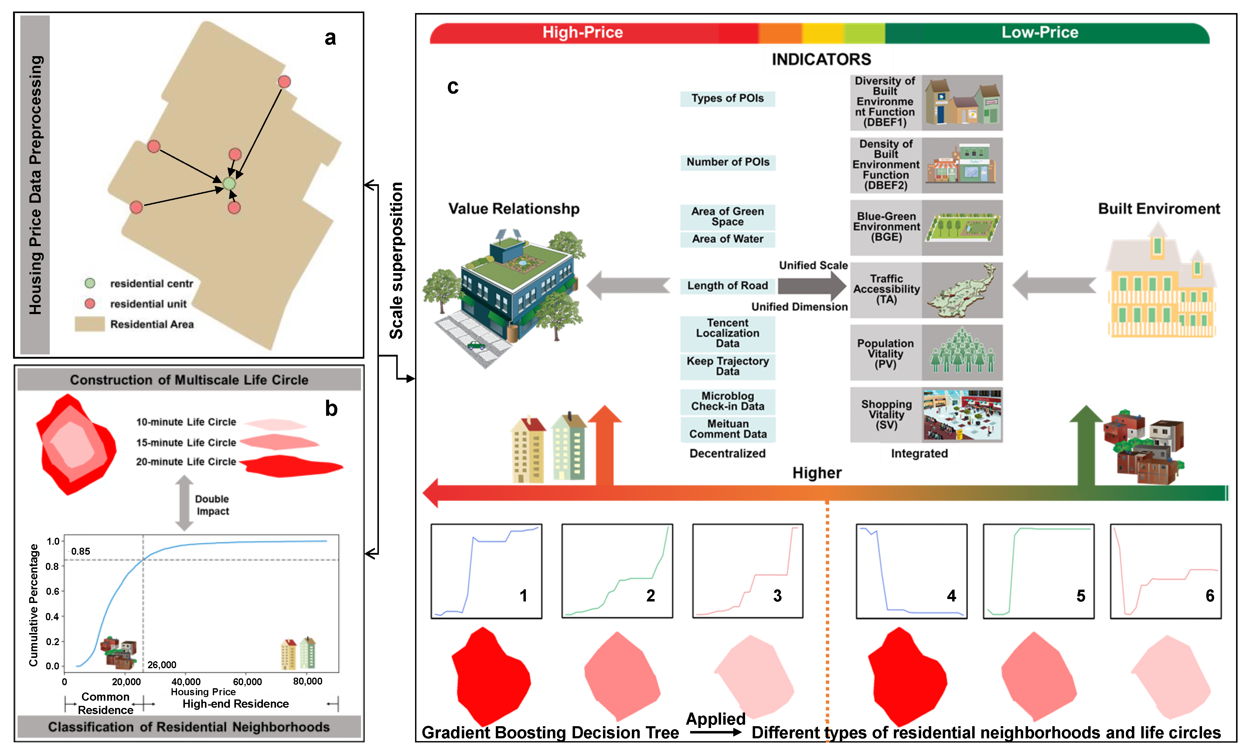
2.1. Research Design

To explore the nonlinear relationship between residential housing prices and the built environment, this study proposes a nonlinear model based on machine learning and examines the contributions and hierarchical effects of various built environment indicators from the perspectives of multiscale life circles and residential differentiation (Figure 1). With the support of urban crowdsourcing data, we unify the scale and dimension of similar multisource data and integrate them into six categories of indicators: diversity of built environment functions (DBEF1), density of built environment functions (DBEF2), blue–green environment (BGE), traffic accessibility (TA), population vitality (PV), and shopping vitality (SV) (Figure 1c). In terms of scale, with changes in walking time and distance, there will be significant differences in people’s perception and experience of the surrounding environment [22,55]. Elias Willberg et al. [8] verified that the 10 min access experience is most affected by differences in age and season sensitivity, while the 20 min difference is the smallest; Li Linbo et al. [56] confirmed this view in a study of public transport station accessibility. Therefore, this study uses the geometric center of the residential neighborhoods to design 10 min, 15 min, and 20 min multiscale life circle catchment areas (the actual travel distances are approximately 660 m, 990 m, and 1320 m, respectively), and according to the cumulative percentage of housing prices and data differences (Figure 1b), the results are divided into common residences and high-end residences. Finally, using the machine learning method of GBDT, we explore the effects of the built environment on housing prices under different life circles and different types of residences (Figure 1c).

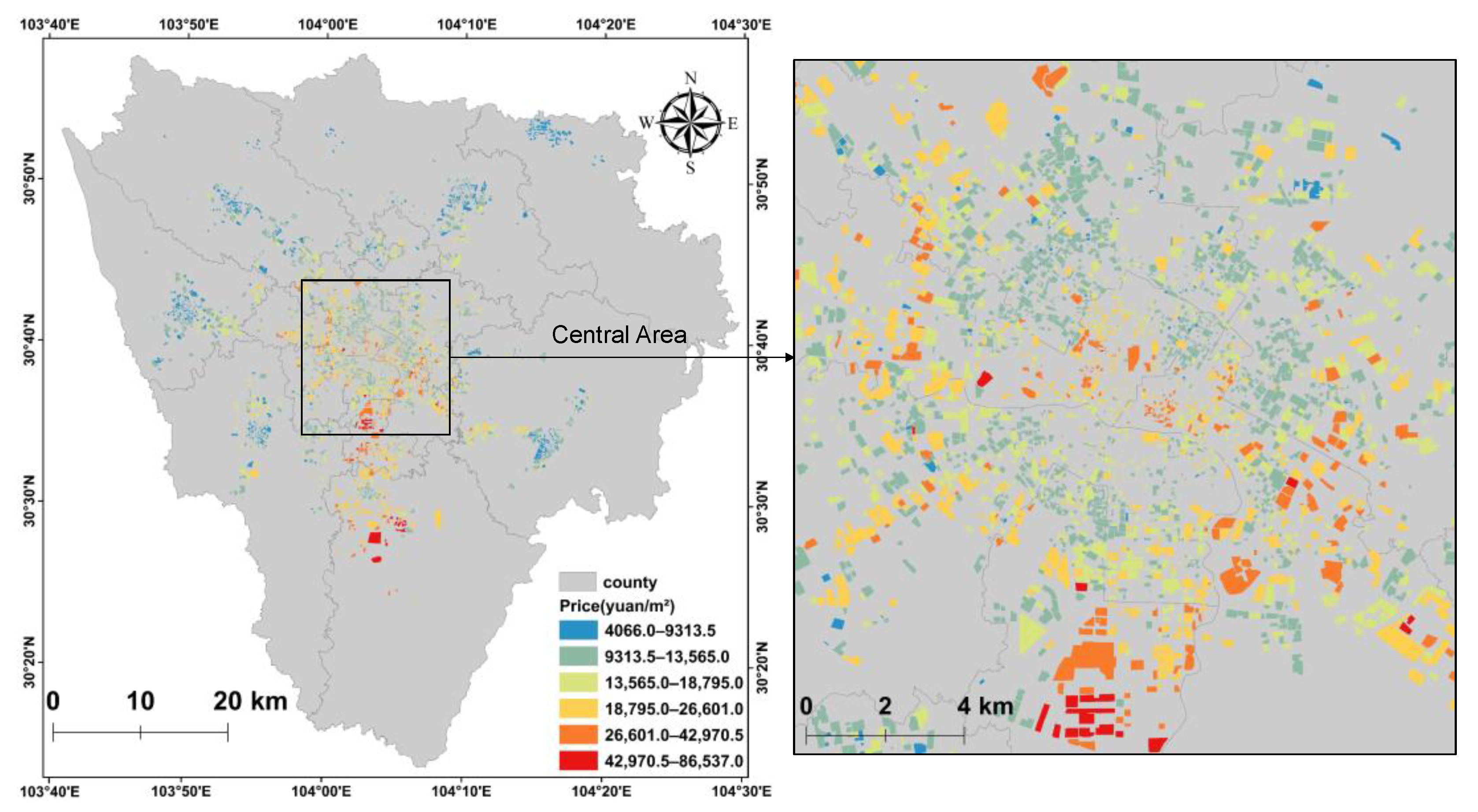
2.2. Overview of the Study Area

Chengdu, a national central city in Western China, has a permanent population of 21.268 million and a built-up area of 1331.1 km², with an average residential building area of 36.57 m² per person. As of 2022, the sales area of commercial housing reached 27.73 million m². The annular spatial configuration of Chengdu city offers significant utility in the establishment of a habitable life circle within rapidly expanding urban landscapes across China. Utilizing Chengdu as a case study, insights garnered therein stand poised to furnish a point of reference for the development of an optimal neighborhood-centric life circle in central hub cities, such as Zhengzhou, Xi’an, Beijing, Shanghai, and others. According to statistics from the Beike housing sales website (https://cd.ke.com/(accessed on 18 November 2022)), the transaction volume of second-hand houses in 2022 was 151,300 units, 8380 units higher than that of new houses in the same period, indicating a high level of activity in the second-hand housing market. Considering that the income gap between the metropolitan and suburban area of Chengdu has significant impacts on housing prices, and that the vast majority of transaction records are concentrated in the metropolitan area, the metropolitan area of Chengdu serves as the study area (Figure 2). This area includes 11 administrative districts, Jinjiang, Qingyang, Jinniu, Wuhou, Chenghua, Xindu, Pidu, Wenjiang, Shuangliu, Longquanyi, and Qingbaijiang, and 2 functional districts, High-tech Zone and Tianfu New Area. Additionally, the varying construction timelines of second-hand houses and new houses introduce inaccuracies to the research findings. Therefore, we opt to focus our research on second-hand houses with higher transaction volumes.

2.3. Data Sources and Processing

2.3.1. Housing Price Data Collection and Processing

The housing price data were sourced from Beike (https://cd.ke.com/ (accessed on 18 November 2022)), China’s largest second-hand housing trading platform, using Python to call the API. Data entries without price attributes were removed, leaving a total of 8083 housing price data entries. Since the transaction prices are recorded on a per-property basis, there are cases where a residential neighborhood has multiple units, but they all belong to the same neighborhood, i.e., the built environment of the living space should be consistent. However, due to differences in construction time, layout, and other factors, price variations can arise. To eliminate this impact, the prices of these residential units were averaged and assigned to the geometric center point of the neighborhoods as the final price (Figure 1a). After processing, there were a total of 5290 residential communities with price attributes (Figure 2). Figure 3 encapsulates the coefficient of variation (CV) of housing prices during the process of data amalgamation for these residential complexes. The mean CV registers at 0.05, with”mere’y 1% of the samples manifesting a CV exceeding 0.5 and 5% of the samples exhibiting a CV surpassing 0.25. This collective profile serves to ensure a notable degree of stability in the property prices across various residential communities, thereby efficaciously mitigating the potential impact stemming from inherent idiosyncrasies of individual developments on pricing dynamics.

2.3.2. Multiscale Life Circle Construction

The construction of a life circle first requires the acquisition of AOI data of the residential area. These data were sourced from Amap (https://www.amap.com/ (accessed on 16 October 2022)), and the geometric center point was extracted using ArcGIS 10.6. QGIS 3.0 software can directly call the isochrone API in the open route service (https://openrouteservice.org/ (accessed on 24 May 2023)). This study used this information to create 10 min, 15 min, and 20 min walking life circles for residential communities with housing price attributes.

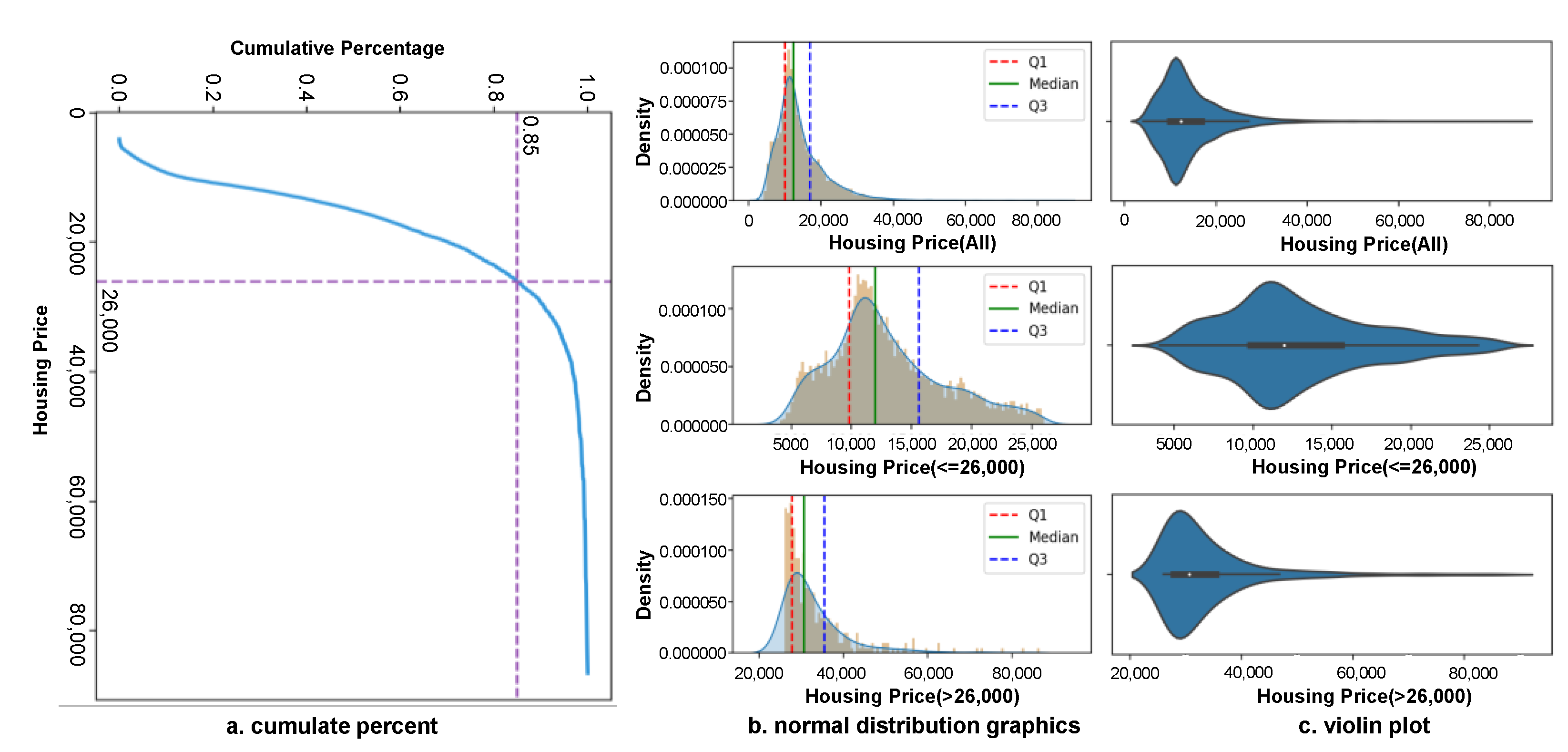
2.3.3. Classification of Residential Neighborhoods

The spillover effect brought about by a prosperous real estate market is crucial to the differentiation of residential spaces [57]. On the one hand, real estate market behavior is strongly influenced by the decision preferences of developers [58], especially the location choices of the built environment [59]. On the other hand, the regulation of housing prices is not entirely controlled by the supply volume of developers but depends on the demand volume of users [60]. Under the dual drive of the market and demand, the housing preferences of different social strata show differentiation, thereby exacerbating the spillover of housing prices [61]. Existing research has decomposed the housing market level from the perspective of data quantile grading [62]. This study comprehensively considers the actual housing market in the Chengdu metropolitan area and finds that when the ratio of houses for sale is close to 85%, the number of houses tends to saturate with increasing housing prices. At this time, the price is approximately RMD 26,000 (Figure 4). Therefore, the dataset is divided into common residences (≤26,000) and high-end residences (>26,000) based on this threshold. Before binning, the overall variance was approximately 7160; after binning, the variance within common residences was approximately 4717, while that within high-end residences was approximately 9015. Additionally, the variance between groups was approximately 5126. Therefore, the binning results preserve the price characteristics of common residences while blurring the uncertainty of the high-end residence group.

2.3.4. Selection of Built Environment Indicators

Open data platforms have enriched the city’s crowdsourced datasets, providing multiple perspectives for the exploration of the urban built environment. In the design of built environment indicators, this paper centers its attention on the formulation of life circle, striving for a semblance of uniformity in the composition of these indicators. This approach not only facilitates the establishment of nonlinear relationships with pragmatic planning significance but also enhances the feasibility of rendering substantive evaluations of the built environment quality tailored to the specific geographical context. Therefore, this study, with residents’ behavioral trajectories as the main focus, pedestrian streets as the dimension, and the scope of the life circle as the guide, comprehensively considers six types of objects: density and types of living facilities, environmental perception, travel ability, shopping vitality, and human flow activities. Living facilities refer to facilities directly related to residents’ production and life, presented in the form of POIs (points of interest), including seven categories: tourism, sports, education, medical, shopping, dining, and transportation [63,64]. Environmental perception uses the area of water bodies and green spaces (blue–green spaces) as an indicator. The blue–green space shows the natural landscape of the living space, which is very important for improvements in the quality of life and the experience of travel [25,65]. Traffic accessibility is exclusively quantified as the total length of road according to the actual range of the life circle. The creation of a life circle is predicated upon isochrones (zones reachable within stipulated timeframes). Hence, the aggregated road length efficaciously mirrors both the connectivity and accessibility of road networks [8,56]. Shopping vitality is based on data collected from China’s mainstream social website Weibo and consumer website Meituan [38,66]. The former reflects the “check-in” consumption behavior of popular places, while the latter provides dining consumption information. Combining the two yields a more comprehensive coverage of consumer trajectories across demographics. Finally, human flow activities are reflected by Tencent’s location data and Keep’s running trajectory data. These data record location information via software. From the perspective of usage frequency, Tencent’s location data collect information at a large scale and the macro level [23,24], while Keep’s data are targeted at micro human flow information at the community neighborhood scale [67,68]. Moreover, the phenomena of morning and evening peaks in fitness jogging behavior enhance the time dimension of the study [19]. Data collection was conducted in the year 2022, encompassing the life circle of various residential communities as the sampling scope.

Table 1. Selection of built environment indicators and data description.

Aspect	Variables	Variables Description	Meaning of Building	Data Sources
Diversity of Built Environment Function (DBEF1)	Types of POIs	Shannon diversity index (SHDI) of tourism, sports, education, medical, shopping, catering and transportation facilities	Measure the supply capacity of service facilities in the life circle [63,64]	Amap open platform (https://lbs.amap.com/ (accessed on 16 October 2022))
Density of Built Environment Function (DBEF2)	Number of POIs	The point density of tourism, sports, education, medical, shopping, catering and transportation facilities (/km2)	Measure the richness of service facilities in the life circle [24,64]
Blue-Green Environment (BGE)	Proportion of Blue-Green Spaces	Proportion of green and water area (km2)	Measure the amount of natural landscape enjoyed in the life circle [25,65]	Map World development platform (https://www.tianditu.gov.cn/ (accessed on 10 August 2022))
Traffic Accessibility (TA)	Road Network Length	Total length of roads within the life circle (km)	Measure the convenience of travel in the life circle [8,56]
Population Vitality (PV)	Tencent Localization Data	Activity density per km2 (/km2)	Measure the spatial vitality in the life circle [24,68]	Tencent map location service platform (https://lbs.qq.com/ (accessed on 14 March 2023))
	Keep Trajectory Data			Keep open platform (https://keep.com/ (accessed on 8 May 2023))
Shopping Vitality (SV)	Weibo Check-in Data		Measure the consumption tendency in the life circle [38,66]	Weibo open platform (https://open.weibo.com/ (accessed on 23 March 2023))
	Meituan Comments Data			Meituan open platform (https://developer.meituan.com/ (accessed on 19 April 2023))

records the descriptions and specific sources of these data, and

Table 2. Index status under multiscale life circle.

Aspect	10-min Life Circle		15-min Life Circle		20-min Life Circle
	Mean	Std	Mean	Std	Mean	Std
Diversity of Built Environment Function (DBEF1)	4.06	0.32	4.19	0.23	4.26	0.18
Density of Built Environment Function (DBEF2)	1276.48	756.93	1188.19	658.30	1116.08	594.29
Blue-Green Environment (BGE)	0.18	0.08	0.18	0.07	0.18	0.06
Traffic Accessibility (TA)	13.80	3.81	13.25	2.93	12.83	2.42
Population Vitality (PV)	335.02	390.18	331.54	367.20	326.07	343.50
Shopping Vitality (SV)	626.81	343.83	621.70	338.08	614.26	332.46

presents the basic situation of the indicators under the 10 min, 15 min, and 20 min multiscale life circles.

2.4. Modeling Method

2.4.1. Kernel Density Estimation

This study first developed a method to convert location data and social media data into spatial vitality based on kernel density estimation. Given the significant population aggregation in shopping malls, especially in central business districts (CBDs), kernel density estimation reflects the spatial density distribution of pedestrian traffic and shopping activities.

To smooth the vitality measurement, we performed kernel density estimation (KDE) on location data, trajectory data, review data, and social media data, outputting the point density in each grid pixel [69]. The calculation of density $\widehat{f}\left(x,h\right)$ is typically based on the bandwidth $h$ and the kernel function, as expressed by Formula (1):

$$\widehat{f}\left(x\right)=\frac{1}{nh}{{\displaystyle \sum }}_{i=1}^n{K}_h\left(x-x_i\right)$$

(1)

where $x_i$ represents various types of point datasets containing coordinates $X$, $Y$, where $i$ takes values 1, 2,…, $n$; $x$ is the center of $X$, $Y$ in each pixel grid; and $h$ is the search bandwidth, i.e., the smoothing parameter. Considering the range of 10–20 min life circles, the bandwidth $h$ is set to 1500 m; $K_h$ is the distance decay kernel function, which can be expressed by Formula (2):

$$K_h\left(x\right)=\frac{exp\left(-\frac{1}{2}{x}^T,x\right)}{\sqrt{2\pi }h}$$

(2)

Given the variations in life circle areas across different scales, the vitality density coverage rate will naturally diverge gradually, potentially undermining the model’s robustness. Furthermore, the data collection time intervals may not be completely consistent. Considering the population’s mobility, density accumulates greater influence over time. As a result, the density is treated as dimensionless and adjusted based on the life circle areas and the collection time, as shown in Formula (3):

$$V=\frac{\widehat{f_S}}{St}$$

(3)

where $\widehat{f_S}$ is the total vitality density within the life circle; $S$ is the area of the life circle; and $t$ is the duration of data collection.

2.4.2. Gradient Boosting Decision Tree

The study also uses the GBDT model to explore the relationship between housing prices and the built environment. GBDT divides samples into multiple subgroups and uses the average value of observations in each subgroup for prediction. Its goal is to simulate real values through the minimum loss function, iterate multiple times, and reduce the prediction error. Compared to ordinary regression models, GBDT has two advantages [18]: (1) it does not demand normality of data and can accommodate variables with missing values; (2) it solves the problem of multicollinearity within the data serves to avert the intercorrelation among the built environment indicators.

GBDT can be used to construct multiple decision trees and, under their joint action, establish an approximate function of response variable y for a set of explanatory variables x, that is, f(x) [24,50]. This method is based on the accumulation of multiple single decision trees h(x; am) to achieve f(x):

$$F\left(x\right)={\displaystyle \sum }_{m=1}^M{f}_m\left(x\right)={\displaystyle \sum }_{m=1}^M{\beta }_{m}h\left(x;a_m\right)$$

(4)

where $a_m$ is the average value of the starting and ending nodes of each split variable in the single decision tree $h\left(x; a_m\right)$ and ${\beta }_m$ is estimated by minimizing the loss L:

$$L\left(y,F\left(x\right)\right)={\left(y-F\left(x\right)\right)}^2$$

(5)

To reduce the possibility of overfitting, a learning rate parameter $\xi$(0 < $\xi$ ≤ 1) is introduced to control the contribution of each base tree:

$$f_m\left(x\right)=f_{m-1}\left(x\right)+\xi {\beta }_{m}h\left(x; a_m\right)$$

(6)

To obtain robust model results, fivefold cross-validation is used during model training, with the main parameters including the number of trees, learning rate, and tree depth. Under the overall sample (housing price data not stratified), this study selected up to 5000 trees, kept the shrinkage parameter at 0.001, and set the maximum depth to 5. After 2000 iterations, the model results were stable and achieved the best effect, with the pseudo R² of the three life circle samples all exceeding 0.5. In the design of housing price hierarchical effect, since the sample was divided into two portions and the data volume decreased, the model was tested in the same way, and, finally, 1000 trees were used. The learning rate was still kept at 0.001, the maximum depth was 4, and the pseudo R² of both common residences and high-end residences exceeded 0.6.

In addition, among many machine learning methods, the decision tree model is particularly outstanding in terms of interpretability [20]. It establishes nonlinear relationships between variables by creating partial dependencies (PDPs), overcoming the inherent “black–box” characteristic of many machine learning models [20,22].

Breiman et al. [70] adopted a method to evaluate the relative importance of factor $x_k$ in predicting responses:

$$I_k^2\left(T\right)={\displaystyle \sum }_{t=1}^{J-1}{\widehat{\tau }}_t^{2}I\left(v\left(t\right)=k\right)$$

(7)

where the sum term is the nonterminal node of the J-end node number; $x_k$ is the split variable associated with node t; and as the number of training iterations increases, ${\widehat{\tau }}_t^2$ continuously reduces the square error value of the prediction result. For the set of decision trees ${\left\{T_m\right\}}_1^M$ obtained via the gradient enhancement method, the average of all additive trees is taken as follows:

$$I_k^2=\frac{1}{M}{\displaystyle \sum }_{m=1}^M{I}_k^2\left(T_m\right)$$

(8)

3. Results

3.1. The Nonlinear Effects of the Built Environment on Housing Prices in a Multiscale Life Circle

3.1.1. The Relative Importance of Multiscale Built Environment Factors

The GBDT model can be used to identify the relative importance of various indicators of the built environment to urban housing prices, that is, the relative contribution of each indicator to the prediction of housing prices during the modeling process. This result serves as a quantitative indicator of the impact. A higher value signifies a greater effect on housing prices. The GBDT model findings demonstrate that all six indicators impact housing prices (

Table 3. The relative importance of built environment factors of multiscale life circle to housing prices.

Independent Features	Relative Importance (%)
	10-min	15-min	20-min	Mean
Diversity of Built Environment Function (DBEF1)	10.67	10.88	15.85	12.47
Density of Built Environment Function (DBEF2)	20.83	19.88	15.59	18.77
Blue–Green Environment (BGE)	15.29	17.14	11.33	14.58
Traffic Accessibility (TA)	4.23	4.27	10.71	6.40
Population Vitality (PV)	14.61	13.79	30.39	19.60
Shopping Vitality (SV)	34.37	34.04	16.12	28.18

), with PV and SV being the most important. In the 10 min life circle, SV exhibits the highest relative importance to housing prices, followed by DBEF2, while TA has the weakest effects. Within the 15 min life circle, SV retains the most important indicator, and the relative importance and order of each indicator are essentially the same as those for the 10 min life circle. Within the 20 min life circle, the relative importance and order of indicators change substantially, with PV becoming the most important. The relative importance of SV, DBEF2, and DBEF1 remains consistent at approximately 16%, while the weakest indicator is BGE.

Overall, SV (28.18%), PV (19.60%), and DBEF2 (18.77%) are the most important indicators within life circles of different scales. Although many studies have confirmed the impact of various built environment factors on housing prices, in the life circle scale, population and consumption affect housing prices most strongly. Within the 10–15 min life circles, the importance of SV and DBEF2 is significantly higher than that within the 20 min life circle. As the life circle expands, the significance of PV grows, and the underlying human flow activities become an important indicator supporting regional housing prices. Conversely, the importance of SV and DBEF2 diminishes, while the importance of DBEF1 rises. This suggests that as the life circle scale expands, DEBEF1 becomes more important than density. A richer built environment function enhances its capacity to cater to the varied living needs of different populations on a larger scale.

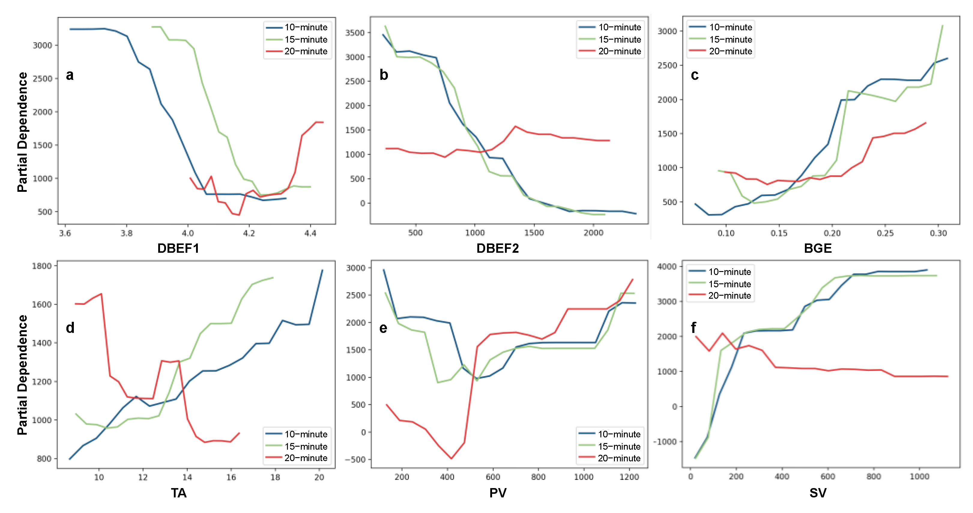
3.1.2. The Nonlinear Relationships between the Multiscale Built Environment and the Housing Prices

The partial dependence plot (PDP) visualizes the nonlinear relationship between different built environment factors and housing prices at different life circle scales (Figure 5), and its trend is consistent with the results of the relative importance analysis. The overall trend of the nonlinear relationship at the three life circle scales is consistent, but there are significant differences in the nonlinear relationship between the 20 min life circle and the 10–15 min life circles at local points.

The partial dependence (PD) analysis reveals a declining trend in the effects of the built environment function diversity and density on housing prices (Figure 5). In the 10–15 min life circles (Figure 5a,b), both DBEF1 and DBEF2 exhibit similar downward trends, starting with a rapid decline and eventually stabilizing with reduced impact. This suggests a threshold hierarchical effect, indicating that the impact on housing prices is greater when the DBEF1 and DBEF2 are at lower levels. As the function density and diversity gradually increase, the impact on housing prices quickly declines until reaching a certain threshold, after which it stabilizes. In the 20 min life circle, the influence of DBEF1 on housing prices slightly increases with the increasing diversity, while the influence of DBEF2 remains stable. In other words, increasing function density does not significantly augment the impact on housing prices. Although the diversity and density of the built environment function have an important impact on housing prices, there is a hierarchical threshold effect. This impact is clearly manifested only when the function diversity and density are insufficient. As the function diversity and density increase, this impact weakens.

The impact of the BGE on housing prices demonstrates an overall upward trend, maintaining a similar trend across the three life circles (Figure 5c). This suggests that as the proportion of BGE area increases, its impact on housing prices gradually strengthens. The most pronounced strengthening trend is observed in the 10 min life circle, followed by that in the 15 min life circle and the 20 min life circle. Notably, the scale difference of BGE local dependence is noticeable. When the BGE area proportion is in the 0.15~0.22 interval, the impact of BGE on housing prices quickly strengthens, and its area proportion increase significantly affects housing prices in the 10–15 min life circles. This result indicates that there is a strong and significant dependence and scarcity effect of BGE on housing prices. It implies that the demand for BGE within the life circle remains unfulfilled, and an increase in BGE can swiftly and significantly affect the changes in housing prices, highlighting the current rigid demand for BGE in life circles. This underscores the rigid demand for BGE in life circles, most notably in smaller-scale ones. Residents envision a highly accessible green environment within a 10 min life circle, where nearby BGE can greatly enhance residents’ happiness and livability. However, the impact of distant large-scale BGE on livability is relatively weak.

The impacts of TA, PV, and SV on housing prices exhibit notable nonlinear relationships (Figure 5d–f), and the local characteristics of dependence are clear. In the 10–15 min life circles, the impact trends of TA, PV, and SV on housing prices are relatively consistent, and the nonlinear trend of the impact in the 20 min life circle changes significantly, indicating a scale effect. In the 10–15 min life circles, the impacts of TA and SV on housing prices show a gradually strengthening trend. The strengthening trend of TA’s impact on housing prices is relatively consistent throughout the value range, among which the strengthening trend of TA in the 15 min life circle is the most significant, suggesting that the relationship between transportation accessibility and housing prices is the most significant at this scale. In the 20 min life circle, the influence of TA shows a weakening trend, indicating that an increase in transportation accessibility beyond a certain distance range will actually reduce its impact on housing prices. This implies that the demand for transportation accessibility for living needs is limited to a specific neighborhood. The impact of SV on housing prices gradually strengthens in the 10–15 min life circles, but its strengthening trend has obvious stages. When SV is in the low-value range (<250), the influence quickly increases; in the middle-value range (250~700), the strengthening trend slows; and in the high-value range (>700), the relationship remains stable. This result suggests that an increase in SV can significantly affect housing prices, particularly when the impact trend is more pronounced in the low-vitality stage. However, as SV continues to increase, the marginal effect on the impact weakens; that is, SV has a high hierarchical threshold effect. The influence of PV on housing prices exhibits a trend of first decreasing and then gradually increasing. The turning point of the impact occurs at approximately 500 in the 10–15 min life circles and approximately 400 in the 20 min life circle. This change implies that there is a threshold in the impact of PV on housing prices. In other words, the impact of low-density PV on housing prices tends to be weaker, while the impact of high-density PV tends to be stronger. This relationship trend holds true across all three life circle scales.

3.2. The Hierarchical Effect of the Relationship between the Built Environment and Housing Prices in a Multiscale Life Circle

3.2.1. Nonlinear Relationship and Hierarchical Effect of the Built Environment

The local dependence of various indicators of the built environment on housing prices varies greatly in the 10 min life circle (Figure 6). The impact of DBEF1 and DBEF2 on high-end residential housing prices is relatively stable, with the impact of functional diversity greater than that of functional density. However, both DBEF1 and DBEF2 exhibit a downward trend in local dependence on common residences and, overall, it is weaker than their impact on high-end residences. Similarly, for BGE and TA, their impact on high-end residential housing prices is stronger than their impact on common residences, and the fluctuation in the trend is also weaker. PV and SV show evident nonlinear trends in their impact on common residences and high-end residences. Overall, as PV and SV strengthen, their impact on housing prices increases, especially the impact of SV on common residences, which increases substantially and quickly surpasses its impact on high-end residences. Overall, within the 10-minute life circle, the impact of different built environment factors on different types of housing shows nonlinear and stratified trends, among which high-end residence housing prices are more dependent on DBEF1, DBEF2, BGE, and TA, while common residence housing prices are more dependent on SV and PV.

Within the 15 min life circle, the differences in the dependence of different types of housing prices on built environment indicators are further highlighted (Figure 7). The impact of DBEF2 on high-end residences is significantly stronger than its impact on common residences, while the impact of DBEF1 on both types of housing prices is similar; the BGE exhibits a nonlinear strengthening trend on the prices of common and high-end residences, while the dependence of high-end residences on BGE is significantly stronger than that of common residences. The impact of TA on high-end residences showcases an overall downward trend, while its impact on common residences is weaker and maintains a stable trend. The impacts of PV and SV on common residences and high-end residences both illustrate a nonlinear strengthening trend, among which the impact trend of SV on the two types of housing prices is relatively similar, both quickly strengthening and then maintaining a stable trend. The impact of PV on high-end residential housing prices is significantly stronger than its impact on common residences, but its impact trend is relatively stable. The impact of PV on common residences showcases a typical nonlinear strengthening trend, indicating that common residential housing prices have a strong dependence on high-density PV.

Within the 20 min life circle, the differences in the local dependence of common and high-end residential housing prices on various indicators of the built environment become more pronounced (Figure 8). Comparatively, except for DBEF1, the impact trends of the remaining built environment factors on housing prices are relatively stable. The impact of DBEF1 on the prices of the two types of housing expresses a stepwise upward trend, with its impact on high-end residences significantly stronger than its impact on common residences. The impact of DBEF2 on housing prices tends to be stable, but it showcases a clear hierarchical effect. This reveals that its impact on high-end residences is stronger than its impact on common residences. Similarly, within the 20 min life circle, the impact of the BGE and TA on housing prices tends to be stable, but the differentiation of their impact on different types of housing prices becomes more pronounced. The impacts of SV and PV on high-end housing prices both sharply decline initially and then become stable. The difference is that the impact of SV on high-end residences is significantly stronger than its impact on common residences, and as the PV increases, its trends with respect to high-end residences and common residences gradually converge.

By comparing the nonlinear relationships between the built environment and the prices of different residences across different life circles (

Table 4. Coefficient of variation of nonlinear relationship between multiscale life circle built environmental indicators and housing prices.

Independent Features	10-min			15-min			20-min
	Unstratified	Common Residence	High-End Residence	Unstratified	Common Residence	High-End Residence	Unstratified	Common Residence	High-End Residence
DBEF1	0.59	0.61	0.63	0.16	0.60	0.11	1.44	0.12	0.48
DBEF2	0.56	0.55	0.56	0.14	0.24	0.21	2.05	0.09	0.75
BGE	0.44	0.29	0.31	0.54	0.15	0.29	0.41	0.24	1.33
TA	0.51	0.67	0.73	1.22	0.20	0.27	0.99	0.44	0.35
SV	0.54	0.37	0.66	1.11	0.23	0.29	1.57	0.54	0.19
PV	1.30	0.08	0.11	0.14	0.22	0.77	0.29	0.03	1.31
Mean	0.65	0.43	0.50	0.55	0.27	0.32	1.13	0.25	0.74

), it can be observed that there is a significant hierarchical effect in the nonlinear relationship between the built environment and housing prices at different life circle scales. Namely, the dependence of prices on the built environment gradually differentiates between grades of housing, and as the research scale expands, the differentiation becomes more pronounced. However, the effects of the built environment on different types of residences tend to be consistent. Specifically, within the 10 min life circle, the trend lines of the impacts of various indicators of the built environment on the prices of both types of residences are generally similar. However, as we expand to the 15 min and 20 min life circles, the differentiation is highlighted and emphasized. For example, for BGE and TA, the difference in their impact within the 10 min life circle is approximately 500, and this difference increases to approximately 1000 within the 15–20 min life circles. This indicates that within the small-scale life circle, the performance of the built environment on housing premiums is not prominent; as the life circle scale expands, after the built environment becomes more diverse and complex, its impact on housing prices shows a clear hierarchical effect. This hierarchical effect is mainly reflected in DBEF2, BGE, TA, and SV. As DBEF2, SV, BGE, and TA increase, this hierarchical effect becomes more pronounced. Furthermore, as the scale expands, the nonlinear relationship between the built environment and housing prices tends to be consistent. For example, DBEF1 and BGE in the 15 min and 20 min life circles have basically the same curve shape, and TA and SV in the 20 min life circle maintain a consistent nonlinear trend.

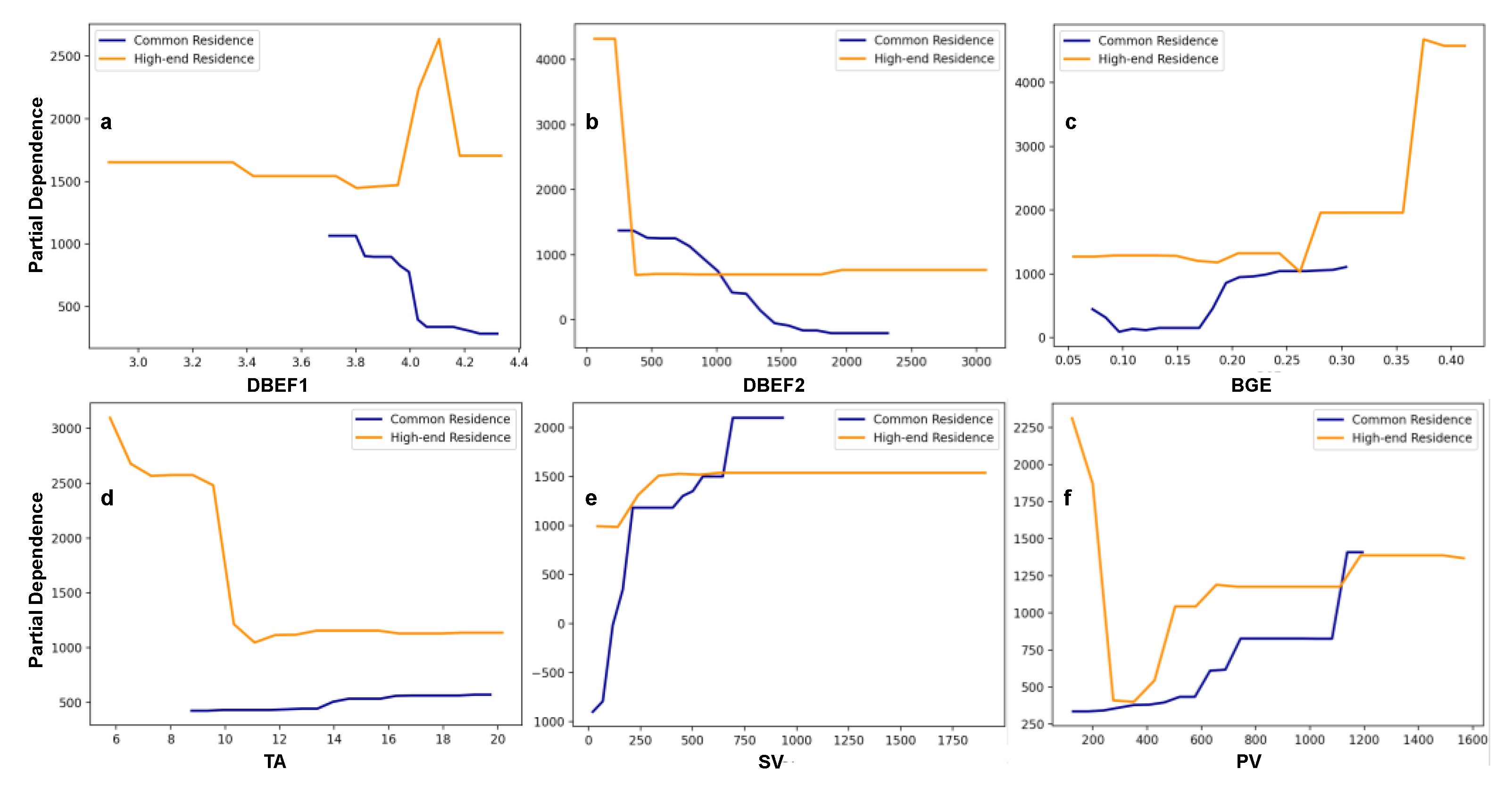
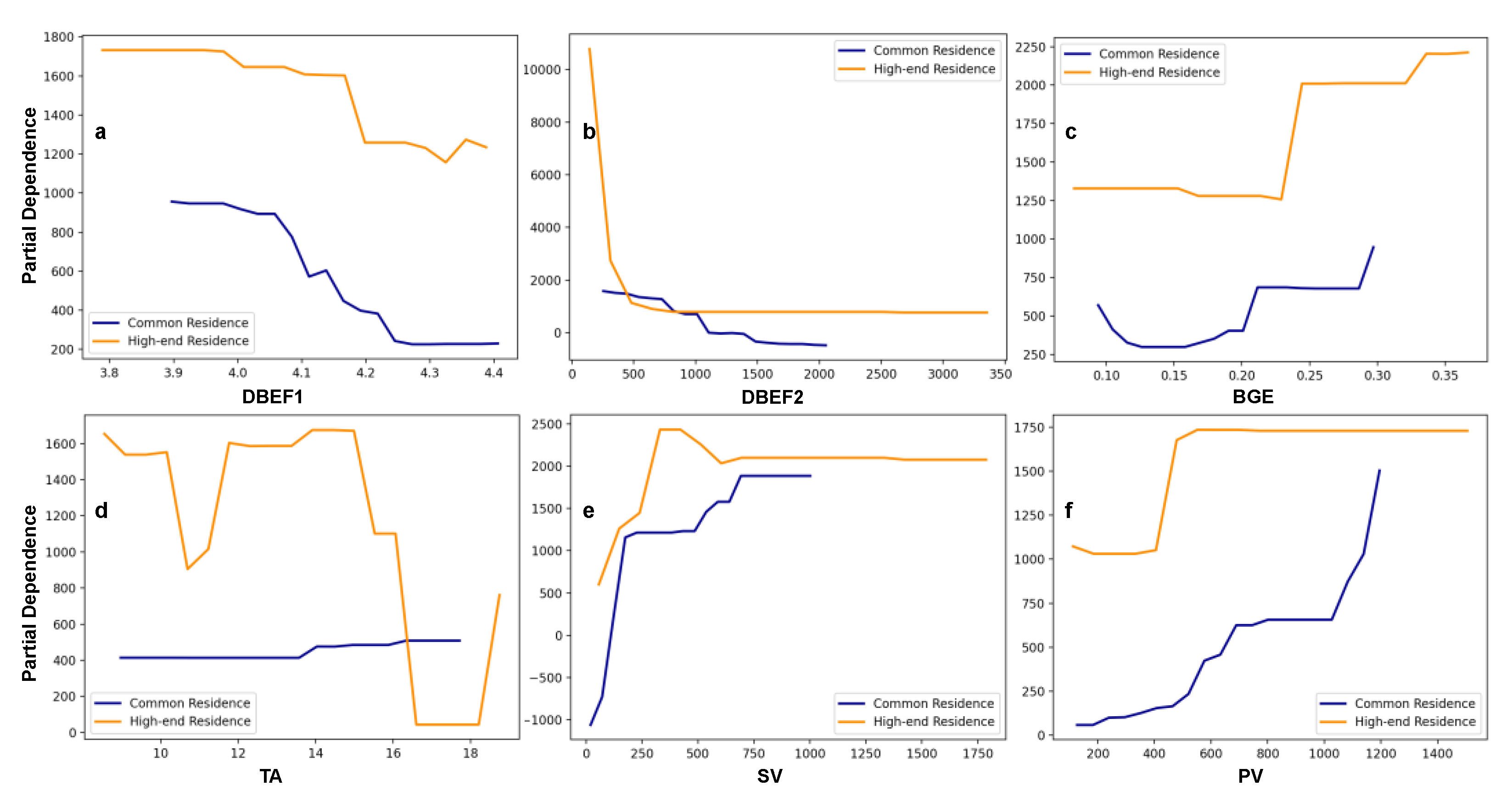
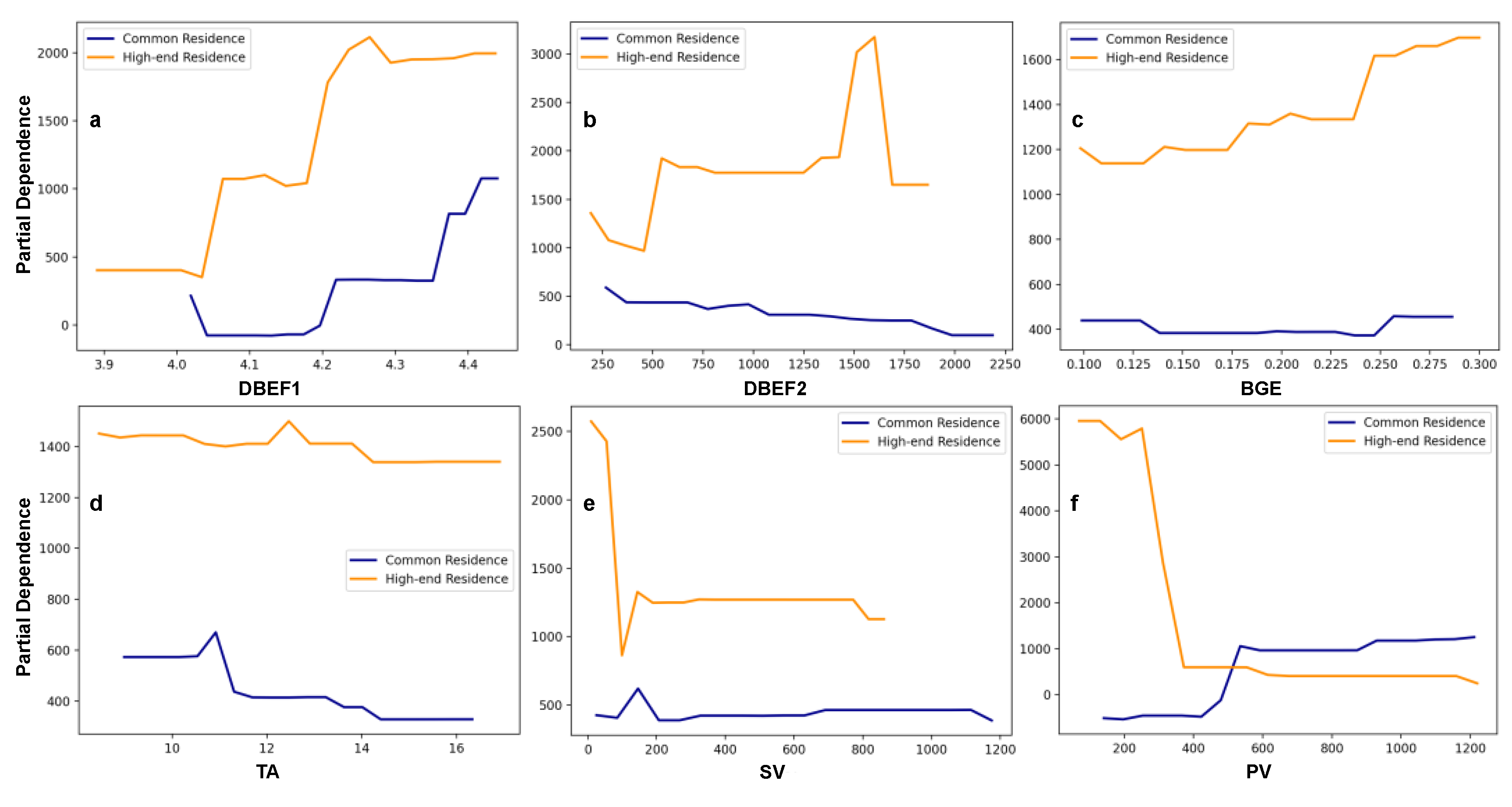
3.2.2. The Effects of the Built Environment on Residential Differentiation in Multiscale Life Circle

Table 5. The relative importance of built environment factors of multiscale life circle to housing prices of different grades.

Independent Features	10-min		15-min		20-min		Mean
	Common Residence	High-End Residence	Common Residence	High-End Residence	Common Residence	High-End Residence	Common Residence	High-End Residence
DBEF1	0.10	0.11	0.11	0.05	0.13	0.12	0.11	0.09
DBEF2	0.21	0.30	0.28	0.37	0.16	0.29	0.22	0.32
BGE	0.18	0.15	0.08	0.09	0.04	0.04	0.10	0.09
TA	0.01	0.13	0.01	0.24	0.07	0.03	0.03	0.13
SV	0.42	0.05	0.43	0.17	0.09	0.15	0.31	0.12
PV	0.09	0.25	0.10	0.07	0.51	0.37	0.23	0.23

displays the relative importance of built environment factors on the prices of different grades of residences within various life circle scales. There are significant differences in the relative importance of some built environment factors on the prices of different grades of residences, and these differences exhibit scale dependency. DBEF1 shows a minor difference in relative importance on the prices of different grades of residences across various life circle scales, while DBEF2 presents a significant difference. Specifically, DBEF2 is less important for the prices of common residences compared to high-end residences. Within a 10 min life circle, the relative importance differs by 0.09, and this difference increases to 0.13 within a 20 min life circle. Thus, as the life circle expands, the impact of DBEF2 on the internal differentiation of residence prices becomes more pronounced. The importance of BGE for common and high-end residences gradually decreases within the 10–20 min life circles, suggesting that residents’ preference for BGEs weakens as the scale expands, and its impact on residential differentiation also weakens with the expansion of the scale. This confirms, to some extent, that the creation of BGEs on a large scale can enhance residential fairness, while the creation of BGEs in small-scale microspaces intensifies residential differentiation. The relative importance of TA varies among different grades of residences as the scale expands. Initially, it increases and then decreases, with the difference reaching its peak within the 15 min life circle. Notably, TA holds the highest significance for high-end residences, while its impact on common residences is relatively weaker. This is mainly because common residence inhabitants prefer to choose public transportation, while high-end residence inhabitants prefer driving, making them more sensitive to nearby road networks. However, within the 20 min life circle, the importance of TA for common residences is significantly higher than its importance within the 10 and 15 min life circles, while the impact of TA on high-end residences is significantly weaker than its impact within the 10 and 15 min life circles. This denotes that the preference for transportation among different types of residence inhabitants varies. As the scale expands, the impact of nearby road networks on common residence inhabitants increases, while the impact on high-end residence inhabitants weakens. This ascertains that the impact of transportation accessibility on residential differentiation exhibits scale dependency, which is mainly manifested through residents’ travel behavior.

Within the 10 and 15 min life circles, the impact of SV on common residences is significantly greater than its impact on high-end residences, with this difference being most pronounced in the 10 min life circle. However, within the 20 min life circle, the impact of SV on high-end residences surpasses its impact on common residences. This change illustrates that SV can significantly influence residential differentiation, and its impact is scale-dependent and closely related to indicators, such as SV and residents’ consumption preferences. The difference in the importance of PV to housing prices is greatest within the 10 and 20 min life circles and smallest within the 15 min life circle. However, within the 10 min life circle, the importance of PV to high-end residences far exceeds its importance to common residences; within the 20 min life circle, the impact of PV on common residences is significantly greater than its impact on high-end residences. This implies that PV is influenced by residential differentiation and varies within different scales; high-end residences are more dependent on PV within smaller scales, while common residences show a more pronounced dependence on PV within larger areas.

A case study in Chengdu shows that built environment factors not only significantly influence residential differentiation but this differentiation also exhibits clear scale dependency, with TA, SV, and PV being the most prominent influencing factors. By examining the impact of various factors on residential differentiation within different scale life circles, it was found that DBEF2 has the most pronounced impact on residential differentiation within the 10 and 15 min life circles, while BGE, TA, SV, and PV have the most pronounced impact within the 10, 15, 10, and 10 min life circles, respectively. This signifies that differences in the built environment within smaller-scale life circles can shape residential differentiation, i.e., housing prices are more sensitive to the impact of the built environment on a smaller scale. When comparing the differences in the impact of various indicators on residential differentiation, the impact of SV within the 10 min life circle on residential differentiation stands out most. This implies that the shopping environment within the built environment has a greater impact on residential differentiation than other environmental indicators. This is because residential preferences are a form of consumption behavior, and different consumption behavior preferences include preferences for residential choice. Residents of high-end residences, benefiting from their socioeconomic advantages, tend to be more sensitive to the consumer environment. Additionally, a high concentration of SV can promote residential premium within the neighborhoods. Notably, this impact is dependent on the scale. As the scale expands, the impact of SV on residential differentiation weakens, i.e., residents’ dependence on SV exhibits proximity.

4. Discussion

4.1. Construction of Life Circle and Residential Equity

The platform economy and the financialization of housing can easily disrupt the fairness of urban development [71], but fairness is not reflected through the market, as the market itself is selective. Instead, it is presented through the needs and life experiences of residents [58,60]. As shown in this study, compared to the six aspects of the built environment, the price advantage of common residences is more reflected in the convenience of life experience, while high-end residences focus on the quality of life. This is similar to the conclusions of most studies [12,38].

The life circle, as the urban space most closely related to residents’ life activities [1], can accurately reflect residents’ life experiences when used to measure the built environment. There are two points worth noting: First, the quantity of built environment factors. This study mentioned that all indicators show a certain hierarchical effect and abrupt change in the process of affecting housing prices, so excessive increases in the quantity of built environment factors cannot play a positive role. Second, the scale of the life circle is vital. Due to individual differences, a fixed life circle range obviously cannot meet the needs of all residents. As the scale increases, the overlap of life circles in various communities will also increase. While improving the efficiency of public resource utilization, it also promotes the group fairness of living space [11,16].

With the urban expansion and gentrification of space development, residential differentiation is inevitable, especially in rapidly urbanizing cities such as Chengdu. From the perspective of built environment indicators, Chengdu, under the background of the park city, shows almost no imbalance in blue–green space [72]. The densities of functional facilities, traffic accessibility, and shopping vitality have become the main contributors to residential differentiation, and the impact of population vitality is most strongly affected by scale effects. Different built environment factors have the best functional spatial scale, and different types of residential neighborhoods also have the best living space scale. Therefore, choosing to break through the existing life circle scale in planning policies (15-min), seeking the best scale that meets the needs of urban development and residential equity, such as based on individual behavior [2] and refining urban units [73], can lead to reasonable planning of living space. Moreover, it is important to grasp the scale of the built environment factors, capture their abrupt changes in the impact on housing prices in the local range, prevent the dramatic manifestation of housing price differences within a large area, and effectively alleviate the degree of residential differentiation in urban areas [33,74].

4.2. Broad Applicability of the Research Framework

The analytical framework proposed in this study exhibits universality, primarily manifesting in two key aspects. First, it can be readily adapted to analyze the influence of built environment factors on housing prices and residential space differentiation across urban spaces of varying scales and dimensions. While this study primarily delves into analysis from the comprehensive lens of the basic life circle, there is an exciting prospect in further dissecting spatial facets into realms, like consumption space, public service space, and social vitality space. Second, the construction criteria for living environments in China are still in the exploratory stage. With the rise of the 5~10 min life circle, the capacity of a 15 min life circle to fully cater to residents’ needs has waned [8,11]. Furthermore, as Chengdu falls within the ranks of emerging first-tier cities in China and possesses a spatial hierarchy akin to cities such as Beijing and Shanghai, this framework is fully applicable to cities sharing similar spatial structures or comparable levels of development.

Moreover, the influx of data, when coupled with the transformative influence of machine learning, has triggered a paradigm shift in traditional urban spatial modeling. The convergence of these factors has led to a formidable driving force behind the modeling and analysis of urban spaces. The potent leveraging of machine learning techniques in handling data has greatly advanced the modeling and analysis of urban spaces. Of particular significance is the establishment of nonlinear relationships, thereby significantly augmenting the interpretability of the model’s independent variables. This analytical approach improves upon traditional geospatial models that struggle to establish definitive functional or linear relationships. Thus, machine learning showcases substantial versatility in urban spatial modeling, capable of application in more intricate and multidimensional subjects of study.

4.3. Study Limitations

In the era of digital smart cities, the advent of crowdsourced data enables a finer exploration and perception of various dimensions within urban environments. This synthesis of data sources empowers us to better grasp the interplay between socioeconomic factors, mobility patterns, and the formation of life circles, thereby enriching our insights and contributing to a more informed urban planning and policy-making discourse.

Notably, because this study offers data-driven modeling and interpretation of the impact of built environment factors on property prices, a complete causal relationship between the two is not fully unified and robust. On the one hand, interpretations should be contextualized with the actual circumstances and domain expertise of the research subject, a common predicament encountered in all machine learning approaches. On the other hand, although machine learning methods drive the interpretability of data modeling, the robustness of this relationship has potential risks [75,76]. If there is an insufficient sample size or the difference between data is excessive, the results will be affected [51,75]. In our study, the determination of PV and SV predominantly relies on smartphone app usage records, inevitably omitting a wealth of user-specific information, such as income, gender, age, and the nuanced temporal variations at destinations, like daytime and nighttime fluctuations. The utilization of more refined multisource urban crowdsourcing data to construct built environment factors emerges as a prospective direction for the future.

5. Conclusions

To conclude, this study combines a gradient boosting decision tree (GBDT) and partial dependence plot (PDP) to use machine learning models to reveal the factors influencing housing prices in the metropolitan area of Chengdu under the guidance of multiscale life circles. With the support of urban crowdsourced data, six types of indicators were selected: diversity of built environment functions (DBEF1), density of built environment functions (DBEF2), blue–green environment (BGE), traffic accessibility (TA), population vitality (PV), and shopping vitality (SV). In addition, this paper considers the dual impact of multiscale life circle and housing price hierarchical phenomena, further revealing the nonlinear relationship between the built environment and housing prices, elucidating the scale, premium, and stability of its impact on the housing market. It provides strong theoretical support for life circle planning, constructing the built environment, and guiding the housing market. The conclusions and understandings are as follows:

(1)

There is a significant nonlinear relationship between the built environment and housing prices. This relationship has hierarchical effects and inflection point effects on each indicator, which has a profound impact on residential premiums. The impacts of SV and PV on housing prices are the most significant, revealing that resident behavior is the main factor of housing pricing on the scale of residential neighborhoods.

(2)

From the multiscale life circle perspective, the impact trend of the built environment on housing prices within a 15 min life circle remains stable; however, after dividing the types of residences, the stability of each indicator’s impact on housing prices is no longer obvious. As the life circle scale increases, the price effects of the built environment on different residences tend to be consistent, but the performance of price differences is more intense.

(3)

The difference in the built environment is the main effecting factor of residential differentiation, and the effect of the built environment has scale dependence. On a small life circle scale, housing prices are more sensitive to the impact of the built environment; on a large scale, the performance of residential differentiation is more obvious, and the influence is greater.

This study makes substantial contributions to existing knowledge in the following three aspects: (1) It reveals the nonlinear relationship between the built environment and housing prices, providing new ideas for the quantitative creation of the built environment indicators. (2) It explores the rationality and importance of multiscale life circle construction, providing a basis for the fine reconstruction of urban space and the creation of a suitable living environment. (3) It clarifies the impact and scale dependence of residential differentiation affected by built environment factors.

This study considers the actual situation of the housing market to explain the scale dependence of the shaping indicators of residential differentiation and clarifies that the performance of built environment factors on housing premiums is different in large- and small-scale life circles. Therefore, whether the scale of life circle planning should be refined from the city as a whole to neighborhood blocks and create different scale life circle standards has become a new topic worthy of attention. It is undeniable that this will help the rational allocation of built environment factors, avoid the local surplus and lack of public resources, avoid the waste of social resources, and improve social fairness.

References

1. Liu, T.; Chai, Y. Daily Life Circle Reconstruction: A Scheme for Sustainable Development in Urban China. Habitat Int. 2015, 50, 250–260. [Google Scholar] [CrossRef]
2. Chai, Y. From Socialist Danwei to New Danwei: A Daily-Life-Based Framework for Sustainable Development in Urban China. Asian Geogr. 2014, 31, 183–190. [Google Scholar] [CrossRef]
3. Han, F.; Tao, D. Evaluation of Residents’ Daily Life Convenience Degree from the Viewpoint of Daily Life Circle, Nanjing. Planners 2020, 36, 5–12. [Google Scholar] [CrossRef]
4. Kang, Y.; Zhang, F.; Gao, S.; Peng, W.; Ratti, C. Human Settlement Value Assessment from a Place Perspective: Considering Human Dynamics and Perceptions in House Price Modeling. Cities 2021, 118, 103333. [Google Scholar] [CrossRef]
5. Qiu, W.; Li, W.; Liu, X.; Zhang, Z.; Li, X.; Huang, X. Subjective and Objective Measures of Streetscape Perceptions: Relationships with Property Value in Shanghai. Cities 2023, 132, 104037. [Google Scholar] [CrossRef]
6. Han, Z.; Li, Y.; Liu, T.; Dong, M. Spatial Differentiation of Public Service Facilities’ Configuration in Community Life Circle: A Case Study of Shahekou District in Dalian City. Prog. Geogr. 2019, 38, 1701–1711. [Google Scholar] [CrossRef]
7. Ministry of Natural Resources of the People’s Republic of China. Spatial Planning Guidance: Community Life; Ministry of Natural Resources of the People’s Republic of China: Beijing, China, 2020. [Google Scholar]
8. Willberg, E.; Fink, C.; Toivonen, T. The 15-Minute City for All?—Measuring Individual and Temporal Variations in Walking Accessibility. J. Transp. Geogr. 2023, 106, 103521. [Google Scholar] [CrossRef]
9. Li, Y.; Chai, Y.; Chen, Z.; Li, C. From Lockdown to Precise Prevention: Adjusting Epidemic-Related Spatial Regulations from the Perspectives of the 15-Minute City and Spatiotemporal Planning. Sustain. Cities Soc. 2023, 92, 104490. [Google Scholar] [CrossRef]
10. Lu, M.; Diab, E. Understanding the Determinants of X-Minute City Policies: A Review of the North American and Australian Cities’ Planning Documents. J. Urban Mobil. 2023, 3, 100040. [Google Scholar] [CrossRef]
11. Logan, T.M.; Hobbs, M.H.; Conrow, L.C.; Reid, N.L.; Young, R.A.; Anderson, M.J. The X-Minute City: Measuring the 10, 15, 20-Minute City and an Evaluation of Its Use for Sustainable Urban Design. Cities 2022, 131, 103924. [Google Scholar] [CrossRef]
12. Chen, F.; Wu, J.; Chen, X.; Nielsen, C.P. Disentangling the Impacts of the Built Environment and Residential Self-Selection on Travel Behavior: An Empirical Study in the Context of Diversified Housing Types. Cities 2021, 116, 103285. [Google Scholar] [CrossRef]
13. Chen, Y.; Men, H.; Ke, X. Optimizing Urban Green Space Patterns to Improve Spatial Equity Using Location-Allocation Model: A Case Study in Wuhan. Urban For. Urban Green. 2023, 84, 127922. [Google Scholar] [CrossRef]
14. Di Marino, M.; Tomaz, E.; Henriques, C.; Chavoshi, S.H. The 15-Minute City Concept and New Working Spaces: A Planning Perspective from Oslo and Lisbon. Eur. Plan. Stud. 2023, 31, 598–620. [Google Scholar] [CrossRef]
15. Fischer, T. Spatial Inequality and Housing in China. J. Urban Econ. 2023, 134, 103532. [Google Scholar] [CrossRef]
16. Liu, W.; Zheng, S.; Hu, X.; Wu, Z.; Chen, S.; Huang, Z.; Zhang, W. Effects of Spatial Scale on the Built Environments of Community Life Circles Providing Health Functions and Services. Build. Environ. 2022, 223, 109492. [Google Scholar] [CrossRef]
17. Wang, J.; Zhao, M.; Ai, T.; Wang, Q.; Liu, Y. Revealing the Influence of the Fine-Scale Built Environment on Urban Rail Ridership with a Semiparametric GWPR Model. ISPRS Int. J. Geo-Inf. 2023, 12, 218. [Google Scholar] [CrossRef]
18. Yan, J.; Wan, Q.; Feng, J.; Wang, J.; Hu, Y.; Yan, X. The Non-Linear Influence of Built Environment on the School Commuting Metro Ridership: The Case in Wuhan, China. ISPRS Int. J. Geo-Inf. 2023, 12, 193. [Google Scholar] [CrossRef]
19. Yang, W.; Hu, J.; Liu, Y.; Guo, W. Examining the Influence of Neighborhood and Street-Level Built Environment on Fitness Jogging in Chengdu, China: A Massive GPS Trajectory Data Analysis. J. Transp. Geogr. 2023, 108, 103575. [Google Scholar] [CrossRef]
20. Xiao, L.; Liu, J. Exploring Non-Linear Built Environment Effects on Urban Vibrancy under COVID-19: The Case of Hong Kong. Appl. Geogr. 2023, 155, 102960. [Google Scholar] [CrossRef]
21. Xiao, D.; Kim, I.; Zheng, N. Recent Advances in Understanding the Impact of Built Environment on Traffic Performance. Multimodal Transp. 2022, 1, 100034. [Google Scholar] [CrossRef]
22. Tao, T.; Cao, J. Exploring Nonlinear and Collective Influences of Regional and Local Built Environment Characteristics on Travel Distances by Mode. J. Transp. Geogr. 2023, 109, 103599. [Google Scholar] [CrossRef]
23. Chen, L.; Zhao, L.; Xiao, Y.; Lu, Y. Investigating the Spatiotemporal Pattern between the Built Environment and Urban Vibrancy Using Big Data in Shenzhen, China. Comput. Environ. Urban Syst. 2022, 95, 101827. [Google Scholar] [CrossRef]
24. Yang, J.; Cao, J.; Zhou, Y. Elaborating Non-Linear Associations and Synergies of Subway Access and Land Uses with Urban Vitality in Shenzhen. Transp. Res. Part A Policy Pract. 2021, 144, 74–88. [Google Scholar] [CrossRef]
25. Zhang, M.; He, J.; Liu, D.; Huang, J.; Yue, Q.; Li, Y. Urban Green Corridor Construction Considering Daily Life Circles: A Case Study of Wuhan City, China. Ecol. Eng. 2022, 184, 106786. [Google Scholar] [CrossRef]
26. Wang, J.; Mu, Y.; Wang, Z. Distribution and Development of Urban Hot Spots in the Internet Era:A Cace Study of Shanghai. Urban Dev. Stud. 2022, 29, 19–26. [Google Scholar] [CrossRef]
27. Niu, H.; Silva, E.A. Understanding Temporal and Spatial Patterns of Urban Activities across Demographic Groups through Geotagged Social Media Data. Comput. Environ. Urban Syst. 2023, 100, 101934. [Google Scholar] [CrossRef]
28. Chua, A.; Servillo, L.; Marcheggiani, E.; Moere, A.V. Mapping Cilento: Using Geotagged Social Media Data to Characterize Tourist Flows in Southern Italy. Tour. Manag. 2016, 57, 295–310. [Google Scholar] [CrossRef]
29. Hwang, S. Residential Segregation, Housing Submarkets, and Spatial Analysis: St. Louis and Cincinnati as a Case Study. Hous. Policy Debate 2015, 25, 91–115. [Google Scholar] [CrossRef]
30. Song, W.; Liu, C. Spatial Differentiation of Gated Communities in Nanjing. Int. J. Urban Sci. 2017, 21, 312–325. [Google Scholar] [CrossRef]
31. Zhang, L.; Zhu, L.; Shi, D.; Hui, E.C. Urban Residential Space Differentiation and the Influence of Accessibility in Hangzhou, China. Habitat Int. 2022, 124, 102556. [Google Scholar] [CrossRef]
32. Omer, I.; Goldblatt, R. Urban Spatial Configuration and Socio-Economic Residential Differentiation: The Case of Tel Aviv. Comput. Environ. Urban Syst. 2012, 36, 177–185. [Google Scholar] [CrossRef]
33. Song, W.; Huang, Q.; Gu, Y.; He, G. A comparison study on residential differentiation at multiple spatial and temporal scales in Nanjing and Hangzhou. Acta Geogr. Sin. 2021, 76, 2458–2476. [Google Scholar] [CrossRef]
34. Tao, Z.; Guanghui, J.; Guangyong, L.; Dingyang, Z.; Yanbo, Q. Neglected Idle Rural Residential Land (IRRL) in Metropolitan Suburbs: Spatial Differentiation and Influencing Factors. J. Rural Stud. 2020, 78, 163–175. [Google Scholar] [CrossRef]
35. Yanbo, Q.; Guanghui, J.; Yuting, Y.; Qiuyue, Z.; Yuling, L.; Wenqiu, M. Multi-Scale Analysis on Spatial Morphology Differentiation and Formation Mechanism of Rural Residential Land: A Case Study in Shandong Province, China. Habitat Int. 2018, 71, 135–146. [Google Scholar] [CrossRef]
36. Li, J.; Huang, H. Effects of Transit-Oriented Development (TOD) on Housing Prices: A Case Study in Wuhan, China. Res. Transp. Econ. 2020, 80, 100813. [Google Scholar] [CrossRef]
37. Liu, Y.; Tang, Y. Epidemic Shocks and Housing Price Responses: Evidence from China’s Urban Residential Communities. Reg. Sci. Urban Econ. 2021, 89, 103695. [Google Scholar] [CrossRef]
38. Tan, M.J.; Guan, C. Are People Happier in Locations of High Property Value? Spatial Temporal Analytics of Activity Frequency, Public Sentiment and Housing Price Using Twitter Data. Appl. Geogr. 2021, 132, 102474. [Google Scholar] [CrossRef]
39. Kortas, F.; Grigoriev, A.; Piccillo, G. Exploring Multi-Scale Variability in Hotspot Mapping: A Case Study on Housing Prices and Crime Occurrences in Heerlen. Cities 2022, 128, 103814. [Google Scholar] [CrossRef]
40. Sayın, Z.M.; Elburz, Z.; Duran, H.E. Analyzing Housing Price Determinants in Izmir Using Spatial Models. Habitat Int. 2022, 130, 102712. [Google Scholar] [CrossRef]
41. Jiang, Y.; Qiu, L. Empirical Study on the Influencing Factors of Housing Price—Based on Cross-Section Data of 31 Provinces and Cities in China. Procedia Comput. Sci. 2022, 199, 1498–1504. [Google Scholar] [CrossRef]
42. Bagheri, B.; Shaykh-Baygloo, R. Spatial Analysis of Urban Smart Growth and Its Effects on Housing Price: The Case of Isfahan, Iran. Sustain. Cities Soc. 2021, 68, 102769. [Google Scholar] [CrossRef]
43. Rosen, S. Hedonic Prices and Implicit Markets: Product Differentiation in Pure Competition. J. Political Econ. 1974, 82, 34–55. [Google Scholar] [CrossRef]
44. Peng, Z.; Inoue, R. Identifying Multiple Scales of Spatial Heterogeneity in Housing Prices Based on Eigenvector Spatial Filtering Approaches. ISPRS Int. J. Geo-Inf. 2022, 11, 283. [Google Scholar] [CrossRef]
45. Rico-Juan, J.R.; Taltavull De La Paz, P. Machine Learning with Explainability or Spatial Hedonics Tools? An Analysis of the Asking Prices in the Housing Market in Alicante, Spain. Expert Syst. Appl. 2021, 171, 114590. [Google Scholar] [CrossRef]
46. Xiao, Y.; Hui, E.C.M.; Wen, H. Effects of Floor Level and Landscape Proximity on Housing Price: A Hedonic Analysis in Hangzhou, China. Habitat Int. 2019, 87, 11–26. [Google Scholar] [CrossRef]
47. Zhang, M.; Qiao, S.; Yeh, A.G.-O. Disamenity Effects of Displaced Villagers’ Resettlement Community on Housing Price in China and Implication for Socio-Spatial Segregation. Appl. Geogr. 2022, 142, 102681. [Google Scholar] [CrossRef]
48. Nishi, H.; Asami, Y.; Shimizu, C. The Illusion of a Hedonic Price Function: Nonparametric Interpretable Segmentation for Hedonic Inference. J. Hous. Econ. 2021, 52, 101764. [Google Scholar] [CrossRef]
49. Wang, Y.; Wang, S.; Li, G.; Zhang, H.; Jin, L.; Su, Y.; Wu, K. Identifying the Determinants of Housing Prices in China Using Spatial Regression and the Geographical Detector Technique. Appl. Geogr. 2017, 79, 26–36. [Google Scholar] [CrossRef]
50. Ding, C.; Cao, X.; Liu, C. How Does the Station-Area Built Environment Influence Metrorail Ridership? Using Gradient Boosting Decision Trees to Identify Non-Linear Thresholds. J. Transp. Geogr. 2019, 77, 70–78. [Google Scholar] [CrossRef]
51. Soltani, A.; Heydari, M.; Aghaei, F.; Pettit, C.J. Housing Price Prediction Incorporating Spatio-Temporal Dependency into Machine Learning Algorithms. Cities 2022, 131, 103941. [Google Scholar] [CrossRef]
52. Čeh, M.; Kilibarda, M.; Lisec, A.; Bajat, B. Estimating the Performance of Random Forest versus Multiple Regression for Predicting Prices of the Apartments. ISPRS Int. J. Geo-Inf. 2018, 7, 168. [Google Scholar] [CrossRef]
53. Rey-Blanco, D.; Zofío, J.L.; González-Arias, J. Improving Hedonic Housing Price Models by Integrating Optimal Accessibility Indices into Regression and Random Forest Analyses. Expert Syst. Appl. 2023, 121059. [Google Scholar] [CrossRef]
54. Delgado-Panadero, Á.; Hernández-Lorca, B.; García-Ordás, M.T.; Benítez-Andrades, J.A. Implementing Local-Explainability in Gradient Boosting Trees: Feature Contribution. Inf. Sci. 2022, 589, 199–212. [Google Scholar] [CrossRef]
55. Hassan, D.K.; Elkhateeb, A. Walking Experience: Exploring the Trilateral Interrelation of Walkability, Temporal Perception, and Urban Ambiance. Front. Archit. Res. 2021, 10, 516–539. [Google Scholar] [CrossRef]
56. Li, L.; Gao, T.; Wang, Y.; Jin, Y. Evaluation of Public Transportation Station Area Accessibility Based on Walking Perception. Int. J. Transp. Sci. Technol. 2023, 12, 640–651. [Google Scholar] [CrossRef]
57. Tsai, I.-C.; Chiang, S.-H. Exuberance and Spillovers in Housing Markets: Evidence from First- and Second-Tier Cities in China. Reg. Sci. Urban Econ. 2019, 77, 75–86. [Google Scholar] [CrossRef]
58. Monkkonen, P.; Deng, G.; Hu, W. Does Developers’ Ownership Structure Shape Their Market Behavior? Evidence from State Owned Enterprises in Chengdu, Sichuan, 2004–2011. Cities 2019, 84, 151–158. [Google Scholar] [CrossRef]
59. Wang, B. Housing Market Volatility under COVID-19: Diverging Response of Demand in Luxury and Low-End Housing Markets. Land Use Policy 2022, 119, 106191. [Google Scholar] [CrossRef]
60. Somerville, T.; Wang, L.; Yang, Y. Using Purchase Restrictions to Cool Housing Markets: A within-Market Analysis. J. Urban Econ. 2020, 115, 103189. [Google Scholar] [CrossRef]
61. Lu, Y.; Li, J.; Yang, H. Time-Varying Inter-Urban Housing Price Spillovers in China: Causes and Consequences. J. Asian Econ. 2021, 77, 101396. [Google Scholar] [CrossRef]
62. Wen, H.; Li, S.; Hui, E.C.M.; Jia, S.; Li, X. What Accounts for the Migrant–Native Housing Price Distribution Gap? Unconditional Quantile Decomposition Analysis in Guangzhou, China. Habitat Int. 2022, 128, 102666. [Google Scholar] [CrossRef]
63. Li, H.; Wei, Y.D.; Wu, Y.; Tian, G. Analyzing Housing Prices in Shanghai with Open Data: Amenity, Accessibility and Urban Structure. Cities 2019, 91, 165–179. [Google Scholar] [CrossRef]
64. Zheng, Z.; Zhou, S.; Deng, X. Exploring Both Home-Based and Work-Based Jobs-Housing Balance by Distance Decay Effect. J. Transp. Geogr. 2021, 93, 103043. [Google Scholar] [CrossRef]
65. Wu, C.; Du, Y.; Li, S.; Liu, P.; Ye, X. Does Visual Contact with Green Space Impact Housing Pricesʔ An Integrated Approach of Machine Learning and Hedonic Modeling Based on the Perception of Green Space. Land Use Policy 2022, 115, 106048. [Google Scholar] [CrossRef]
66. Hu, L.; He, S.; Han, Z.; Xiao, H.; Su, S.; Weng, M.; Cai, Z. Monitoring Housing Rental Prices Based on Social Media:An Integrated Approach of Machine-Learning Algorithms and Hedonic Modeling to Inform Equitable Housing Policies. Land Use Policy 2019, 82, 657–673. [Google Scholar] [CrossRef]
67. Karusisi, N.; Bean, K.; Oppert, J.-M.; Pannier, B.; Chaix, B. Multiple Dimensions of Residential Environments, Neighborhood Experiences, and Jogging Behavior in the RECORD Study. Prev. Med. 2012, 55, 50–55. [Google Scholar] [CrossRef]
68. Huang, D.; Tian, M.; Yuan, L. Sustainable Design of Running Friendly Streets: Environmental Exposures Predict Runnability by Volunteered Geographic Information and Multilevel Model Approaches. Sustain. Cities Soc. 2023, 89, 104336. [Google Scholar] [CrossRef]
69. Huang, J.; Obracht-Prondzynska, H.; Kamrowska-Zaluska, D.; Sun, Y.; Li, L. The Image of the City on Social Media: A Comparative Study Using “Big Data” and “Small Data” Methods in the Tri-City Region in Poland. Landsc. Urban Plan. 2021, 206, 103977. [Google Scholar] [CrossRef]
70. Breiman, L.; Friedman, J.H.; Olshen, R.A.; Stone, C.J. Classification and Regression Trees, 1st ed.; Routledge: Oxfordshire, UK, 2017; ISBN 978-1-315-13947-0. [Google Scholar]
71. Zhang, M.; Luo, Z.; Qiao, S.; Gar-On Yeh, A. Financialization, Platform Economy and Urban Rental Housing: Evidence from Chengdu, China. Appl. Geogr. 2023, 156, 102993. [Google Scholar] [CrossRef]
72. Zhang, Z.; Ma, G.; Lin, X.; Dai, H. Accessibility in a Multiple Transport Mode Urban Park Based on the “D-D” Model: A Case Study in Park City, Chengdu. Cities 2023, 134, 104191. [Google Scholar] [CrossRef]
73. Guo, L.; Bi, Y.; Huang, J.; Zheng, C.; Hu, G.; Wang, G. Multi-scale Comparison and Analysis of Jobs-housing Spatiale Characteristics in Big Cities—Taking Wuhan as an Example. Urban Plan. Forum 2018, 5, 88–97. [Google Scholar] [CrossRef]
74. Batchelor, D. Refining Urban Design Governance: An Investigation of the Urban Design Assessment Processes in Aotearoa New Zealand. J. Urban Des. 2023, 28, 1–20. [Google Scholar] [CrossRef]
75. Luo, T.; Wang, J.; Fu, T.; Shangguan, Q.; Fang, S. Risk Prediction for Cut-Ins Using Multi-Driver Simulation Data and Machine Learning Algorithms: A Comparison among Decision Tree, GBDT and LSTM. Int. J. Transp. Sci. Technol. 2022, 12, 862–877. [Google Scholar] [CrossRef]
76. Sotomayor, L.N.; Cracknell, M.J.; Musk, R. Supervised Machine Learning for Predicting and Interpreting Dynamic Drivers of Plantation Forest Productivity in Northern Tasmania, Australia. Comput. Electron. Agric. 2023, 209, 107804. [Google Scholar] [CrossRef]
Figure 1. Research framework and technical route of this paper. (a) calculate the average price of residential units and display it in the residential center. (b) construct multiscale life circle and classify residential neighborhoods. (c) establishes the composition of the built environment indicators and the nonlinear relationship driven by GBDT. In which, figures 1–3 are conceptual diagrams depicting the nonlinear relationship between built environment indicators and housing prices for high-end residences under different scale of life circle, while figures 4–6 represent common residences. The same color lines represent the same scale of life circle.)
Ijgi 12 00371 g001
Figure 2. Overview of the study area and housing price in residential neighborhoods.
Ijgi 12 00371 g002
Figure 3. The heterogeneity of housing prices in residential neighborhoods.
Ijgi 12 00371 g003
Figure 4. Chengdu metropolitan housing market division results.
Ijgi 12 00371 g004
Figure 5. Nonlinear relationship between the built environment factors and housing price in different life circles. (a) DBEF1. (b) DBEF2. (c) BGE. (d) TA. (e) PV. (f) SV.
Ijgi 12 00371 g005
Figure 6. The nonlinear relationship between the built environment and the price of different grades of housing in the 10 min life circle. (a) DBEF1. (b) DBEF2. (c) BGE. (d) TA. (e) SV. (f) PV.
Ijgi 12 00371 g006
Figure 7. The nonlinear relationship between the built environment and the price of different grades of housing in the 15 min life circle. (a) DBEF1. (b) DBEF2. (c) BGE. (d) TA. (e) SV. (f) PV.
Ijgi 12 00371 g007
Figure 8. The nonlinear relationship between the built environment and the price of different grades of housing in the 20 min life circle. (a) DBEF1. (b) DBEF2. (c) BGE. (d) TA. (e) SV. (f) PV.
Ijgi 12 00371 g008