Spatiotemporal Predictive Geo-Visualization of Criminal Activity for Application to Real-Time Systems for Crime Deterrence, Prevention and Control

Abstract

This article presents the development of a geo-visualization tool, which provides police officers or any other type of law enforcement officer with the ability to conduct the spatiotemporal predictive geo-visualization of criminal activities in short and continuous time horizons, according to the real events that are happening: that is, for those geographical areas, time slots, and dates that are of interest to users, with the ability to consider individual events or groups of events. This work used real data collected by the Colombian National Police (PONAL); it constitutes a tool that is especially effective when applied to Real-Time Systems for crime deterrence, prevention, and control. For its creation, the spatial and temporal correlation of the events is carried out and the following deep learning techniques are employed: CNN-1D (Convolutional Neural Network-1D), MLP (multilayer perceptron), LSTM (long short-term memory), and the classical technique of VAR (vector autoregression), due to its appropriate performance in the multi-step and multi-parallel forecasting of multivariate time series with sparse data. This tool was developed with Open-Source Software (OSS) as it is implemented in the Python programming language with the corresponding machine learning libraries. It can be implemented with any geographic information system (GIS) and used in relation to other types of activities, such as natural disasters or terrorist activities.

1. Introduction

The high costs associated with delinquency and criminality are, to a greater or lesser extent, known to every society [1,2]. As such, considering the constant work that law enforcement, public security agencies, and investigators throughout the world carry out, it is clear that efforts should be directed towards the creation of tools, policies, and strategies for the deterrence, prevention, and control of this type of activity. Such strategies also make it possible to detect their displacement patterns; this is perhaps one of the best ways to address these issues, save lives, and avoid consequences of all kinds. This is the case for tools that allow for the prevention or prediction criminal activity, which can be applied to real-time scenarios and situations.

The article shows the development of a tool based on this concept. It offers police units or any other type of law enforcement officer a spatiotemporal predictive geo-visualization of criminal activities with a short time horizon using feedback from real events that are happening; these are used to perform the retraining of the predictive model and the following forecasts. Thus, forecasts are made continuously, in real-time, and with a reduced error rate. It is applicable to geographical areas, time slots, and dates of interest, either according to individual event codes or to groups of event codes.

The tool was created using real data from Santiago de Cali (Colombia) that were provided by the Colombian National Police (PONAL), the entity in charge of ensuring public safety in the country. The tool thus enables not only the deterrence of criminal activities but also an increase in situational awareness and the improvement of future projections and agility and efficiency in the tactical and strategic decision-making processes of the PONAL, as a consequence of the reaction to these events [3,4,5,6]. This includes the distribution and management of police resources, with a focus on deployments and patrolling [7,8], particularly when there are not enough staff resources [9].

For the creation of this tool, Python programming language open-source software was used. The system performs a continuous spatial and temporal correlation of the events, and several deep learning techniques are employed, including CNN-1D (Convolutional Neural Network-1D), MLP (multilayer perceptron), LSTM (long short-term memory) and the classic VAR (vector autoregression) technique, due to its suitable performance in the multi-step and multi-parallel forecasting of multivariate time series when the data are sparse. The developed tool is adaptable to any other city or geographical location; it can be used with real data to obtain forecasts in real- time or with data from other types of activities, such as natural disasters or terrorist activity, if they are properly converted to the format used by the tool [10,11,12]. It can also be implemented with any geographic software. This tool is innovative and useful because the method used combines necessary features that can be applied to the architecture of real-time systems, and it allows security to be strengthened in cities, favoring the objectives of a safe city, which is one of the main focuses of smart cities [13]. Thus, this research contributes to the fulfillment of the international commitments of the Sustainable Development Objectives (SDO), according to the United Nations, particularly the following objectives: “11: Sustainable cities and communities” and “16: Peace, justice and strong institutions” [14].

2. Works Related to the Concept of Spatiotemporal Predictive Geo-Visualization

The prediction of when and to what extent all kinds of events and activities could happen, whether these events are human, natural, or otherwise, requires that this information be represented graphically. The interaction of these events constitutes a wide source of information that allows observers, analysts, investigators, and security and control agents to achieve greater accuracy in future projections and to undertake more efficient decision-making in relation to crime deterrence, prevention, and control, allowing for enhanced situational awareness.

As a consequence, the capabilities of spatiotemporal predictive geo-visualization have been investigated in relation to various applications, from observations for the prevention and early warning of natural disasters, such as floods [15], to predictive crime surveillance [16,17]. Therefore, development approaches depend largely on the specific needs to be satisfied. Such is the case for the spatial visualization of conflict hotspots using statistical tools [18,19,20,21], mapping by street segments [22], using contrast patterns to predict spatiotemporal events [23], using multimodal data for event prediction with deep learning tools [24,25,26,27,28], applying temporal geospatial analysis to event classification [29,30] and near-repeat and risk terrain modeling [31].

However, none of these development areas integrate tools that allow for the geo-visualization of forecasts of criminal activity by geographical areas, time slots, and dates, making use of the maximum amount of real data available and in a useful timeframe, such as real time. Moreover, considering that the data are sparse, if they are filtered by individual event codes or groups of event codes, this sparsity is increased further.

To achieve this goal, it is initially necessary to determine the spatial dependency between the locations of the events and the temporal dependency among them. This maximizes the likelihood of the provided forecasts. Therefore, efforts that might be useful in terms of the stated needs include: the geo-visualization of forecasts based on spatial clustering to reflect the characteristics of adjacent terrains [32,33,34,35,36]; forecast geo-visualization for sparse data [37,38,39,40]; the geo-visualization of the forecasting of criminal activities using machine learning and deep learning techniques [34,35,36,39,40,41,42,43]; event forecasting using classical, improved classical, machine learning, and deep learning techniques for multivariate time series [44,45,46,47,48,49,50,51,52,53,54,55,56,57,58,59,60]; and, finally, multivariate time series forecasting with sparse data [61,62,63,64,65].

However, none of the currently developed strategies are able to make use of the now huge amount of real available data provided by security agencies when performing geo-visualizations of criminal activity forecasts in real-time, where the data are correlated in time and space and allow for activity data filtering by zones, time slots, and dates. As a consequence, the work presented in this paper constitutes an architectural proposal for a real-time system that fills the aforementioned research gap and satisfies the needs detailed above.

3. Development of an Effective Tool for the Spatiotemporal Predictive Geo-Visualization of Activity for Real-Time Systems

The Colombian National Police (PONAL) divides cities and towns into quadrants, which are variable areas of extended land that are divided in a non-physical way according to the ratio of population density directly proportional to the armed forces or number of police officers at their service [66]. The quadrants are served by police stations and CAIs (immediate action commands) [66].

Considering this strategic division of police control and the fact that, like Colombian cities and towns, any geographic area can be divided into hypothetical quadrants, the intervention described here is generic, since it can be used for any other place. This grouping of terrain into grids that represent the division into quadrants of any police jurisdiction is the first step in creating a tool for spatiotemporal predictive geo-visualization, since this grouping of areas into sub-areas allows for the correlation of the events that have occurred within each sub-area relative to the others.

The entire process described in this section was undertaken using the open-source programming language Python, which has a large number of mature, community-proven libraries providing visualization, numerical calculations, data analysis, and prediction modules for machine learning and deep learning, as well as classical techniques for multivariate time series.

3.1. Sources of Information and Pre-Processing

Through confidentiality agreements, the PONAL has provided years of data regarding criminal incidents associated with the area of jurisdiction of the city of Santiago de Cali. The first step in preprocessing the data is carried out based on the PONAL database system, where data cleaning is performed to generate a sub-database, eliminating unconfirmed or erroneous events that could have been captured, and extracting the necessary fields, including the timestamp (date and time), latitude, longitude, and event code (case code). After this first step, the next one consists of carrying out a data cleaning and data wrangling process, which basically adapts the geographic coordinate format and the timestamp forma, and performs the organization by timestamp [67]. This process results in a database with the format shown in Figure 1.

Once this process is established, databases can be queried by any time range (date and time) and by any extension of the geographical area of the jurisdiction of the PONAL (latitude and longitude). Analysts and commanders, or any other user, can request from the system the data of smaller or larger areas and, within the chosen area, the range of the temporary date and time data, according to their interests. At this point, the dataset is ready to be used.

3.2. Geographic Spatial Grouping of the Observation Area for Its Correlation

Once the observation area has been defined by its geographic coordinates of latitude and longitude and its event data are ready to be used, a grid bounded by these geographic coordinates is created. This latitude and longitude grid system allows the observation area to be divided into sub-areas, so that, when one or more criminal activity events are detected within each sub-area, they are represented and counted within it as in a density map. In turn, this also facilitates the correlation of events between adjacent sub-areas when it is necessary to generate forecasts, as, following this approach, there is a univariate time series for each of the sub-areas and, therefore, a multivariate time series of the same size as the resolution of the entire grid. This is discussed further in the section titled “Data Forecasting and its Spatiotemporal Geo-Visualization”.

The observation zone can be as wide as the analyst requires in terms of the geographic extension, and the grid division can have the resolution that the analyst chooses according to the observation needs: see Figure 2a. This grid should be placed as a layer over the geographical map of the observation area on the Geographic Information System (GIS) in which the spatiotemporal predictive geo-visualization tool will be used, as shown in Figure 2b. In other words, the concept described in this article constitutes a tool that acts as a plug-in that can be adapted to any GIS through its API (application programming interface). Here, the GIS used is the one integrated into the real-time systems of the PONAL [67].

For the case of PONAL-specific use, and since it refers to spherical coordinates on the terrestrial globe, we created a grid of 40 squares on the latitudinal axis (approximately 896,625 m each) and 25 squares on the longitudinal axis (approximately 1,087,344 m each at the northern latitude and approximately 1,087,704 m at the southern latitude). However, it is important to reiterate that these values are used for this case, but this grid resolution value can be adjusted to the monitoring needs of any geographic territory as required by commanders, analysts, or users in general.

3.3. Temporal Grouping of the Criminal Events of the Observation Area for Correlation

Regardless of the size of the geographic segment chosen as the observation area, the analyst can also select the preferred time range (date and time) in which to analyze this area. Thus, for the same observation area, a different time range for analysis could be chosen—for example, one year, two years, a few months, etc.—as well as precisely choosing exactly which dates are required.

The temporal grouping of criminal ”vent’ In the observation area within the chosen time range is performed, and this temporary grouping is achieved by reorganizing the dataset as a multivariate time series, as follows: the frequency of the multivariate time series is defined as how often the measurement of the cases that occurred will be sampled, and the amount of time within which events in each frame will be represented is defined. For the case considered here, the spatiotemporal predictive geo-visualizer shows the criminal events that occurred during a 30 min period, in frames that are updated every 10 min. Consequently, the frequency of the multivariate time series is 10 min [67].

The above point implies that, according to this choice of values, in each representation of a frame, there will be an overlap of cases of 20 min; that is, the representation of the second frame will again show the cases that occurred in the last 20 min of the previous frame [67]. It is designed in this way with the aim of generating continuity and ease in the forecasting algorithms.

However, it must be clarified that these two parameters have been specified as shown for this case by initially selecting random values and adjusting them by trial and error until finding those that served the intended purpose. Therefore, it is clear that these parameters can also be adjusted according to the requirements of a given scenario, and there is even the possibility of using parameters that do not generate overlaps [67].

Figure 3a shows an example of a 3D multivariate time series, and Figure 3b shows an example of a 2D multivariate time series, once the dataset is rearranged as a multivariate time series the frequency of which will correspond to the value of 10 min.

In Figure 3a, each colored box represents a sub-area of the entire observation area, and each color represents a different density of events. In Figure 3b, each univariate time series, named “SerTemp_x”, represents each of the sub-areas.

In Figure 4, an example is shown where the graphical representation of some frames was randomly taken to show how the tool provides visualization capabilities up to this stage. That is to say, it shows the density of criminal events by sub-areas for each time measured, frame by frame, within a complete observation area (in the example, this is the entire jurisdiction of the PONAL over the city of Santiago de Cali). This geo-visualization also helps users, analysts, and commanders to verify whether the chosen area, its resolution, and the analysis time range are adequate for their objectives or if it would be preferable to modify those parameters.

3.4. Data Forecasting and Its Spatiotemporal Geo-Visualization

A truly useful crime event prediction model for the objectives that this tool proposes must:

• Make forecasts continuously, for short time horizons, and in a useful timeframe as close as possible to real time.
• Be frequently retrained using the largest amount of data from real events in such a way that it not only enhances the forecasts’ reliability but also allows commanders and analysts to observe possible trends in criminal activity more precisely.
• Be as simple as possible, so that its computational cost does not become an obstacle to its proper functioning and model overfitting risks are avoided.
• Provide the visualization of criminal activity forecasts on a map and with timelines.

In accordance with these requirements and as stated in the previous sections, by grouping the data on criminal activity events spatially and temporally, multivariate time series are obtained by the unification of all the univariate series that make up each of the sub-areas of the observation area. In other words, there is a multivariate time series of data that is made up of several univariate time series equal to the number of sub-areas that the resolution of the grid contains, since each univariate time series corresponds to the density of the criminal events in each sub-area. The frequency of the entire multivariate time series is 10 min for this case: see Figure 3.

Grouping the densities of criminal activity events, both spatially and temporally, in a multivariate time series, has the following advantages:

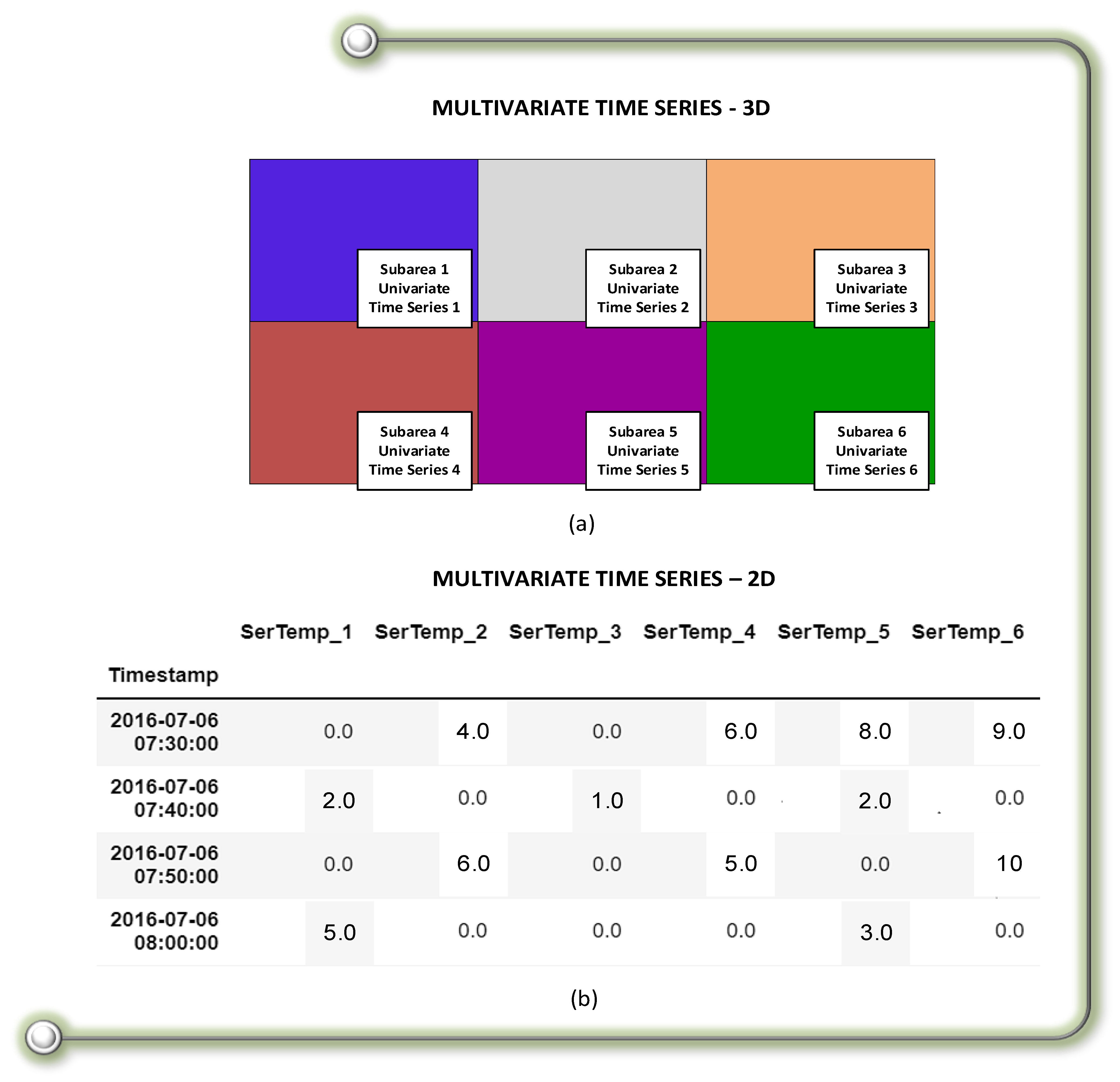
• Spatial correlation is achieved between the sub-areas of the observation area when forecasting future events, as each of the univariate time series conforms with the densities of criminal events in each of the sub-areas. Prediction algorithms take this spatial relationship into account, without the need to provide the location parameter (latitude and length) as a predictor variable.
• Temporal correlation between the sub-areas of the observation area is achieved when forecasting future events, as each of the univariate time series is fitted with the densities of the criminal events of each of the sub-areas. Prediction algorithms take this temporal relationship into account, without the to provide the timestamp parameter as a predictor variable.

This means that the prediction algorithms can be used for multivariate time series, with the predictor variables being the values of the densities of criminal events for each sub-area. This simplifies the model and helps to speed up forecast convergence, but without giving up the spatial and temporal correlation of these events, as these two correlations are essential for the forecast’s reliability. That is, within an observation area, it is only possible to correctly forecast the shift in activity if the events of each of the sub-areas that make it up are correlated with each other.

To carry out prediction tests of criminal activity events, an observation area of 10 quadrants is considered (with the parameter values already chosen in Section 3.2 and Section 3.3), which is the approximate area of jurisdiction of a police station in a city; the analysis considers a time frame of approximately two years, but, again, it must be stated that these parameters are adaptable to any other given scenario. Another important factor to consider is the percentage sparsity of data, which can be checked visually by users in the tool, since the choice of prediction algorithms largely depends on this.

Bearing in mind that, in the proposed use case, all the criminal activity data that occurred in the observation period are used, i.e., no filters are applied by case code, the results show that the data exhibit a sparsity of 0.9871357368590777. In this test, the closer the result is to 1, the higher the dispersion, so it can be concluded that, in this case, we are dealing with data that present a high percentage of zero values when making forecasts for the future. This calculation was performed in Python according to the following formula:

Sparsity = 1.0 − (count of non-zero values within the data)/total size of the data

This feature makes sense, as criminal activity fluctuates according to zones, time slots, and dates, even more so when providing the ability to filter criminal activity events by event codes; this is so that an analyst or commander can request, for example, only the fight cases, or the fight cases added to the property damage cases, and so on.

There is, then, a sparse-type multivariate time series. Regarding the size of the resolution of the quadrants chosen for the observation area, the prediction variables are the integer values of the densities of the criminal activity in each of the sub-areas or in each univariate time series to which it conforms. According to the figures shown above, a scale from 0 to 10 was chosen, with 0 being the absence of events (transparency or the absence of color) and 10 being the maximum concentration of events (black color). It should be noted that the values of this scale can be readjusted if necessary.

The multivariate time series does not have exogenous variables, only endogenous ones; that is, for each univariate time series that makes up the multivariate series, forecasts are required. In addition, it is a high-frequency multivariate time series, since the frequency of the series is 10 min. Additionally, it is multi-parallel, because the forecast of a step (or period), is equivalent to the forecast of a step of the value of the densities of the events in each one of the sub-areas (quadrants) of the observation area, in multi-parallel. This means that the time series is not only multivariate but also multi-parallel. It is then stated that the prediction time horizon or one-step forecast, with which this tool is designed, is 10 min (see Figure 5).

Since the objective is to achieve continuous forecasts, with short time horizons and in a timeframe as useful as real-time, while the model benefits from using large amounts of real data to continuously train itself and to make new forecasts, Figure 6 shows the overall work loop and the requirements for achieving this capability.

According to the example, if the model were trained using the observations made up to 16:10 h, then it would start its forecast operation with the first step showing the observations made up to 16:20 h, and the second forecast step would show the observations made up to 16:30 h. These forecasts would be geo-visualized by commanders and analysts on the geographic map of the observation zone. However, time goes on and the real-time system continues to collect data from actual events within that first time interval of the first forecast step (between 16:10 h and 16:20 h). Therefore, once 16:20 h is reached, the real-time system has the events up to that moment and can store them in the database of the tool (thus increasing it). Therefore, the model can be retrained with these data, and two forecast steps are generated with the new actual data added.

Meanwhile, the geo-visualization has not stopped showing the forecast between 16:10 h and 16:30 h, so, when the model retrains and performs a new two-step forecast, (this time the first one spans until 16:30 h and the second until 16:40 h), the system updates, overwriting the forecast until 16:30 h and displaying the results for the interval until 16:40 h, acting in this way for each of the forecast steps. This gives the observer the feeling of continuity and real time in the forecasts being shown; however, behind the scenes, it is in fact constantly being updated and is using as much real data as possible as it is gathered. This is a highly useful approach for the PONAL environment, as it would notably improve situational awareness and future projections and, therefore, agility and efficiency in police decision-making processes. This is because, among other things, it allows commanders and analysts to observe the trend of the displacement of criminal activity in certain places, either in general, for isolated crimes, or for groups of crimes.

For this ability to be achieved by a system, a model must be able to:

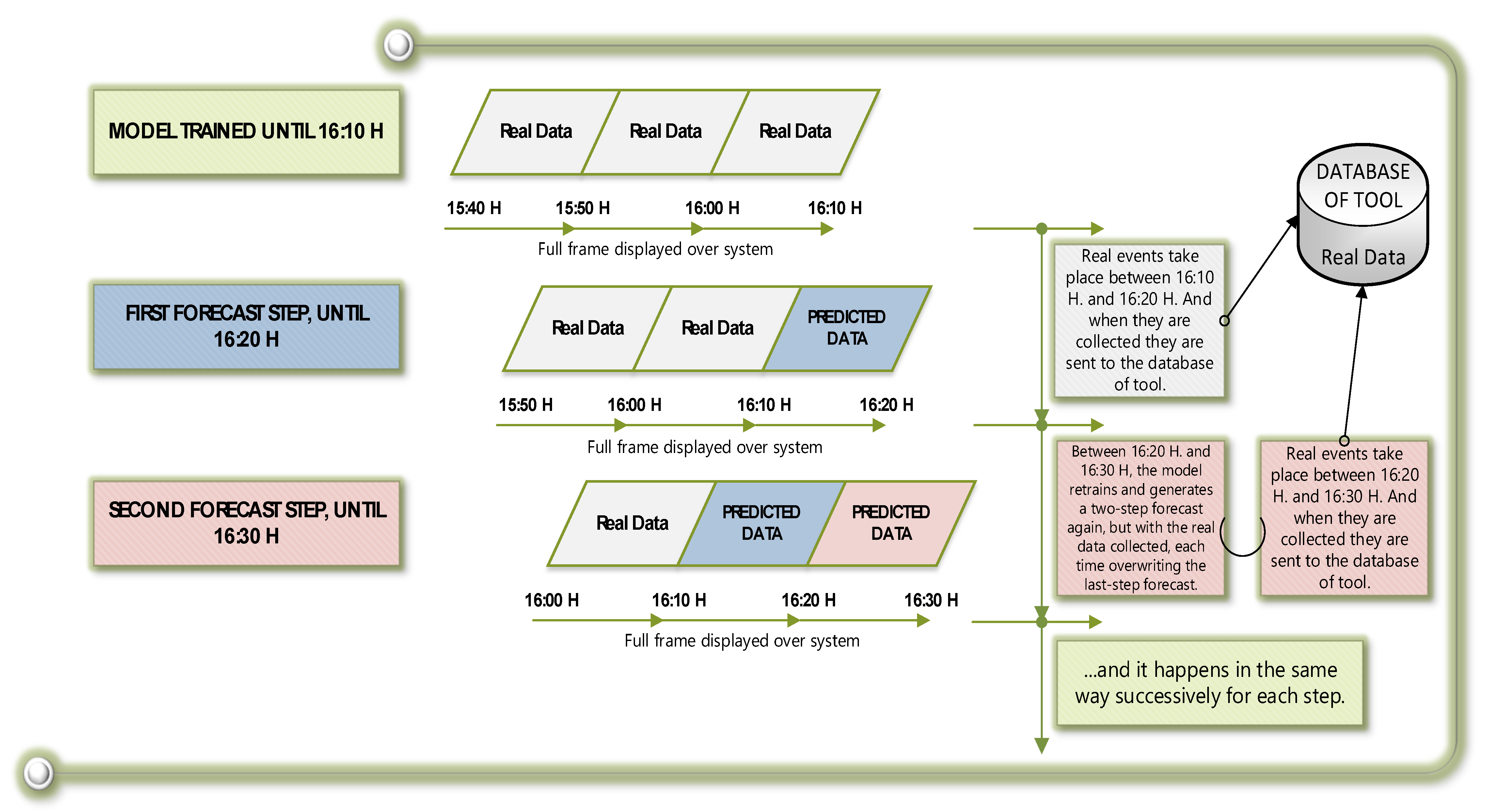
• Be retrained and generate multi-parallel forecasts in a time shorter than the duration of one forecast step of time, that is, in a time shorter than the frequency of the multivariate time series, which, in this case, is 10 min.
• Have the capacity to generate reliable forecasts for a time horizon of at least two steps at a time, since, with single-step forecasts, continuity in geo-visualization cannot be realized. This is because the time slot will not be long enough to collect new information, retrain the model, and generate new forecasts.
• Be as simple and efficient as possible so that everything described above can be fulfilled.

As described up to this point, the conclusive guidelines for the choice of prediction algorithms are set, as shown, by the geo-visualization system’s real-time requirements, and the restrictions of the real data under consideration. For example, not all prediction algorithms for multivariate time series that are able to forecast in multi-parallel will work properly when applied to high-sparsity datasets. The choice of predictive algorithms is also driven by two key features of time series data, namely:

• Seasonality: the multivariate time series discussed here does not present seasonality, especially as it is a multivariate high-frequency sparse-type time series.
• Stationarity: the multivariate time series discussed here turns out to be stationary, so there is no need to perform any type of transformation on the data to achieve it. Stationarity was tested using the Dickey–Fuller test.

3.4.1. Baseline Model

To start testing with the prediction algorithms that may be useful for the purposes of this work, a forecast or baseline model must be established to determine whether the classic models, machine learning, or deep learning are useful and contribute to the achievement of a truly reliable future forecast. In the case of multivariate time series, it is better to establish a naïve reference model, naïve implying that such a forecast will provide observations directly, without any processing; this is also called a persistence forecast due to the observations’ persistence. There are also other possibilities for establishing these baseline models, such as, for example, making averages of some previous observations and using them as a forecast, for which the time series dataset must be transformed into one suitable for supervised learning problems, that is, in the form of inputs (X) and outputs (y). However, the main concern is to find and choose the baseline model that presents the least errors, to be compared with the performance of more elaborate models in order for its value to be assessed, since any model that performs worse than the baseline model should be discarded. On the contrary, if a model improves the forecast error of the baseline model, this is definitely a model that can be considered as a solution to the forecasting problem.

In this case, tests were carried out, with ample sufficiency, to find the best baseline model; it was found that the naïve model of one (1) to one (1) persistence, that is, the model that used the observations of the step of time just before each of the univariate series, was the best for predicting the observations of the next time step of each of the univariate series. This was the model with the lowest error result, because of this, this was chosen as the baseline model and its error metric was as follows, Figure 7:

General information about the results of the models and the testsconducted:

• Time series are a particular case of stochastic processes; therefore, their models are also usually stochastic. This means that they present a certain randomness in their parameters, which is why, when training a model, the values of the error metrics may vary. The implication here is that, when measuring the performance of one of these models, several tests are carried out and the error metrics are averaged. That is, the average is considered the performance value of the model. As a consequence, the values of the error metrics of the models shown in the following sections correspond to the average values of the operation of each model.
• Once the requirements of the system and also those of the predictive models and its forecasts are clarified, the description of the models offered below is based on the methodology of taking all those that meet the initial requirements, according to the nature of the data, and gradually discarding those that do not exceed some thresholds based on the performance criteria. In other words, all possible models are tested, and a filter is used for those where the operation does not meet the needs of the data and of the system, in order to continue working on adjusting only those that provide the expected functionalities.
• For each model, the walk-forward validation technique was used; in this way, not only was the error metric calculated, but the time spent by each model in retraining and generating new forecasts was also verified.
• A model can be considered useful if its two-time-step forecast error metric is less than the reference model’s error metric.

3.4.2. Classical Models for Forecasting Multivariate Time Series

Classical models for forecasting time series are those developed specifically for these purposes; they are SARIMAX models since, in this case, the data are multivariate time series, so the classical models to apply are the –Vector-SARIMAX or V-SARIMAX models. According to the fact that the resulting multivariate time series of data for this case is stationary and non-seasonal, where all its variables are endogenous, it is possible to exempt the usage of components of integration “I”, seasonality “S”, and exogenous variables “X” of the classical vector forecast models for time series V-SARIMAX. As the test option in classical methods, for this case, the VARMA models and their possible combinations (VAR, VMA, and VARMA) are used.

However, it should be noted that we are dealing here with sparse-type data, which implies that, if a sub-area within the observation area is chosen where all the values of the densities of criminal activity are zero, throughout the analysis time range, none of these models will be functional. In other words, VARMA and its derivatives have the restriction that they work only if none of the univariate time series that make up the multivariate time series are completely zero.

VARMA (vector autoregressive moving average) and VMA (vector moving average) models: when performing simple initial tests on these two models (of order 1), the VARMA and VMA models were discarded since, when trained and when forecasts were requested, their convergence took a long time and its error metric did not improve on that of the reference model. It should be recalled that the time convergence between the training and the generation of forecasts of two time steps is required to be a maximum of 10 min so that the system can work properly in the real-time systems of the PONAL, in this case.

Classical Model for Multivariate Time Series, SPARSE type: the classic model for sparse-type multivariate time series, VAR-SPARSE (vector auto-regressive sparse), which is only available for the R programming language through its libraries “bigtime” [68], and “sparsevar” [69], was also tested. However, it was not functional because, even for a small multivariate time series, its convergence was very slow and it took hours to converge. In addition, its consumption of RAM (random access memory) was too high and not justified by the satisfactory performance of the model.

VAR (Vector Autoregressive) model: On the other hand, the VAR model generated a result that improved the error metric of the reference model, and the retraining time and generation of new forecasts were much shorter than 10 min. The result of the VAR model was, Figure 8:

The results were achieved by taking into account that the input data used were raw (without any type of transformation), without the support of the GPU (graphic processing unit and its powerful parallelization capabilities), and by allowing the model to automatically take the order that it considered best for its operations.

Therefore, it can be concluded that this model represents a solution to the problem addressed here, as it works better than the reference model even in a forecast with a time horizon of two steps at a time. It can also be retrained and can generate at least this two-step forecast in a multi-parallel mode in less time than the frequency of the multivariate time series (10 min). This allows for the generation of the predictive continuity proposed by the system that defines this tool; however, it must be remembered that this model is linear. Therefore, it will only work well with stationary time series and it does not work when some sub-area or a univariate time series within the observation area presents a density of cases equal to zero.

3.4.3. Machine Learning (Including Deep Learning) Models for the Forecast of Multivariate Time Series

Random Forest Model: the Random Forest algorithm allows for multi-parallel forecasting for multivariate time series of the sparse type. This is possible for one (1) to one (1) models (taking a previous observation to forecast an observation in the future), and for models that can take several previous observations (X) to forecast several steps into the future (y). Its convergence (training time and forecast generation) is approximately two (2) minutes without the support of the GPU (graphic processing unit). Raw data can also be used, and its only additional requirement is the transformation of the dataset time series to one suitable for supervised learning problems, that is, in the form of inputs (X) and outputs (y).

However, although Random Forest fulfills all the requirements to address all the forecasting needs of this work, its error metric never improved that of the reference model, even after all the possible changes were made within its parameters and all the possible combinations of inputs and outputs for the forecast were assessed. On the contrary, with certain combinations of parameters, the consumption of RAM was too high and without results to justify it. With Random Forest, the best error metric obtained was in the 4 (four) to 3 (three) model, that is, four inputs (X) and three outputs (y) and its value was: RMSE = 0.498. For this reason, the model was discarded.

Deep Learning Models for Multivariate Time Series Forecasting: for time series forecasting, deep learning techniques promise several outstanding benefits, such as:

• The automatic learning of linear and non-linear relationships.
• Learning time structures that present data such as trends and seasonality.
• The handling of long sequences and noisy data.
• Theulti-parallel forecasting of several input and output steps without making assumptions about mapping functions.
• Operating with datasets with missing and sparse values, among others.
• Finally, although the stationary time series represents an advantage, it is not a mandatory requirement for its use.

This scenario is can be tested as a solution in the case that concerns us here, where the deep learning algorithms that specialize in handling sequences and therefore time series are CNN-1D (Convolutional Neural Network-1D), MLP (multilayer perceptron) and LSTM (long short-term memory), with its different variants and combinations of variants Vanilla-LSTM, Stacked-LSTM, Bidirectional-LSTM, CNN-LSTM, and ConvLSTM.

To carry out tests with these algorithms, the data were left raw (without any type of transformation), it was necessary to transform the time series dataset to one suitable for supervised learning problems, that is, in the form of inputs (X) and outputs (y). The performance results of the models shown here were supported by approximately 11% GPU usage.

1.

MLP (multilayer perceptron): this is a simple neural network model that offers an excellent solution for this prediction problem. Figure 9 shows the configuration, the network diagram, and the results of this neural network.

Therefore, it can be concluded that this neural network model is suitable as a solution for the system proposed here, given its simplicity, rapid convergence, efficiency, and error metric, which improves on the reference model even for a two-step forecast.

2.

CNN-1D (Convolutional Neural Network-1D): in general, convolutional neural networks, whether 1D, 2D, or 3D, are designed to preserve spatial structures in raw input data; this is called representation learning. CNNs manage to extract the characteristics of the data regardless of how they are produced, since they remain invariant with the position of the objects and the distortion of the scenes. The CNN-1D, which retains these beneficial features, is ideal for time series forecasting, since time series are sequences of observations that can be treated as one-dimensional images from which the model can extract its main elements, mapping a sequence of earlier observations from the raw data as the input to one or more future observations as the output.

Figure 10 shows the configuration, the network diagram, and the results of the CNN-1D model that offered the best solution for this prediction problem.

Therefore, it can be concluded that this Neural Network model can be considered adequate as a solution for the system proposed here, given its convolutional neural network 1D features and its error metric, which improves on the reference model even for a two-step forecast.

3.

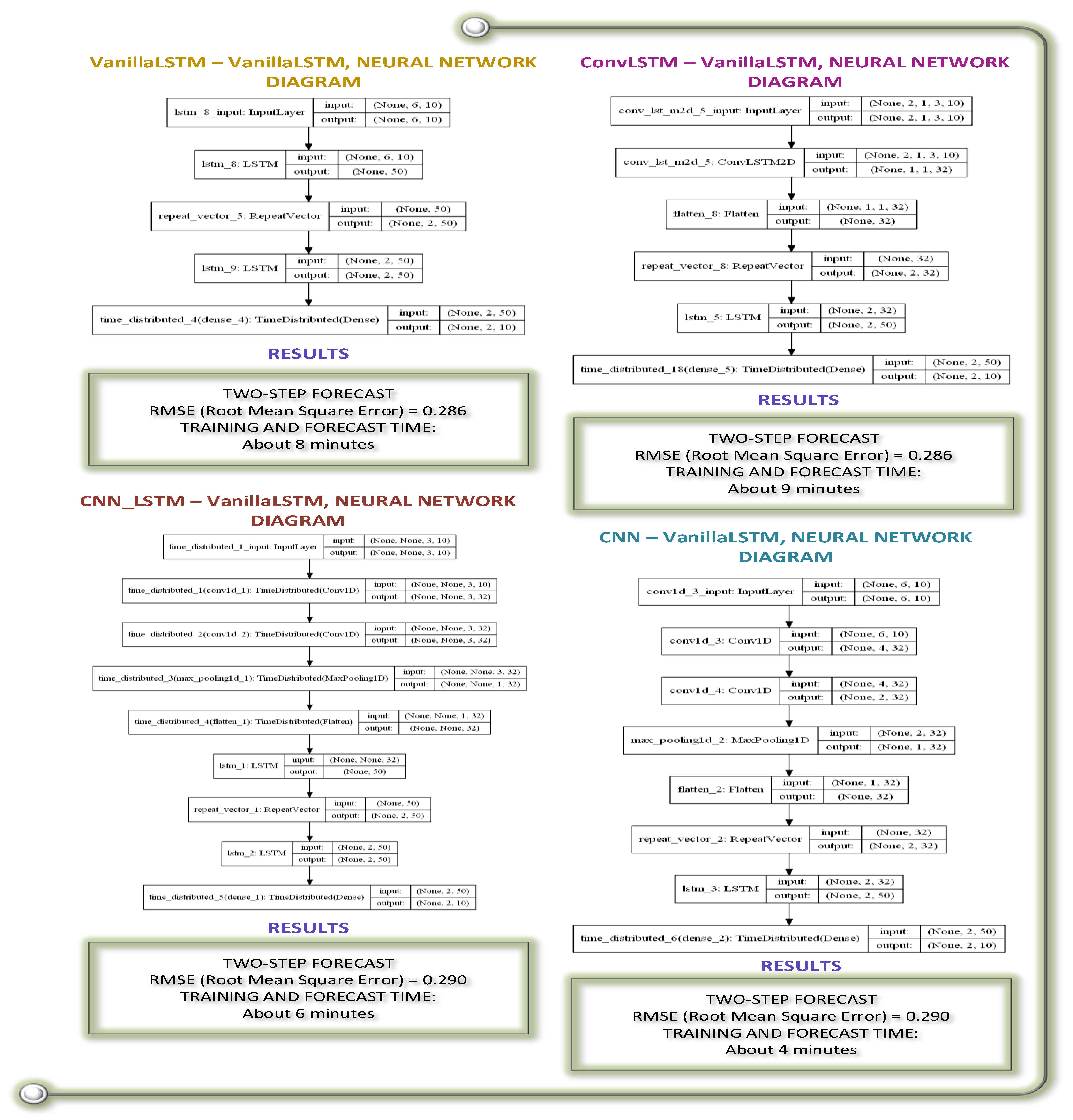
LSTM (Long Short-Term Memory): by their nature, LSTM neural networks read one-time steps from the sequence at a given time and create the representation of that internal step to use as learned context when making forecasts. In other words, LSTM neural networks offer native support for sequences such as time series. The LSTM models that offer viable solutions for this prediction problem according to their convergence (training time and forecast generation), the possibility of forecasting at least two steps, and an acceptable performance that would improve the performance of the reference model, with data in Float 32, are:

Univector output models:

• The Vanilla-LSTM model
• The CNN-LSTM model
• The ConvLSTM model

Figure 11 shows the diagrams of these neural network models and their results.

Encoder-Decoder type models for Multivector output:

• (VanillaLSTM—VanillaLSTM) model.
• (ConvLSTM—VanillaLSTM) model.
• (CNN_LSTM—VanillaLSTM) model.
• (CNN—VanillaLSTM) model.

Figure 12 shows the diagrams of these Neural Network models and their results.

These models are slightly more complex and, although their convergence lays within the established limits, it is a little higher. However, it can be concluded that taking these models into account can be very useful, since, depending on the data, one model or another could fit better. The summary of the results of the LSTM models is as follows, Figure 13:

Figure 14 shows a summary of the main results of the described models.

3.4.4. Forecast Geo-Visualization

A geo-visualizer shows a data forecast on the geographic information system (GIS) of the real-time systems of the PONAL, or any other GIS, in terms of the coordinates of latitude and longitude. However, to show the detail of the system, Figure 15 presents a geo-visualization of the comparison between the real data and the predicted data, scaled in parts of the grid since this parameter is also adjustable.

4. Results and Discussion

It transpires that the concept proposed here, of using the spatiotemporal predictive geo-visualization of criminal activity for real-time systems, is a highly useful tool; it can be used in any geographical location and is applicable to any kind of activity if the data are adapted to the format shown (e.g., terrorist activity and natural disaster activity). This concept allows commanders, analysts, or other relevant users to constantly spatiotemporally geo-visualize the forecasts of the criminal influx in areas of interest, based on the desired dates and time ranges, as well as according to individual event codes or groups of such codes. These achievements were made possible by methodology established in this paper, whereby generating multi-step forecasts (in this case, two-step forecasts) allows the system to update itself by overwriting the last forecast step, and a forecasting environment is created that gives the user the perception of forecasting in real-time. In addition, this forecast is made even more reliable thanks to the use of the largest amount of real data that exist and the flexible ability for users to define their parameters. This also provides the possibility of analyzing the trends and the displacement of the activity considered.

Artificial intelligence techniques were used to make these forecasts; this study is specifically framed within the field of deep learning and, in this work, all the possible techniques for forecasting sparse-type multivariate time series with multi-parallel forecasting were compiled for the solution of this problem. However, it must be noted that the research on the modeling and forecasting of multivariate time series remains an open field and there is still a long way to go. Therefore, the objective of this research was not to focus on these predictive techniques but to concentrate on the operating methodology that is required for spatiotemporal predictive real-time systems geo-visualization tools and to search for those algorithms, techniques, and models that allow for reliable forecasting under the operating parameters discussed in this paper.

The results of this work show that it is possible to develop a spatiotemporal predictive geo-visualization tool for criminal and terrorist activities that is aligned with the mission and strategic objectives of an entity in charge of ensuring security; up to now, this was not feasible in the context of the PONAL. However, there are technical challenges to its implementation that cannot go undiscussed.

In the context of the proposed work, it is necessary to make forecasts by areas with certain extensions in accordance with the tactical and strategic operation of the PONAL. However, in a larger scale deployment, we must considered the operation of forecasting algorithms for sparse-type multivariate time series, which, according to their nature, will work better or worse depending on the size of the series. There must be other developments and integrations with other sources of geo-information, such as the GIS used by other agencies that would use the tool. In addition, another challenge relates to the computational capacity requirements of map, database, and predictive model processing, which may arise from this tool. To overcome these challenges in the context of PONAL, we may benefit from approaches such as cloud-type solutions or solutions with centralized processing in a local data processing centre (CPD) with parallel processing capacity with the support of GPUs with compatibility with CUDA^® from NVIDIA^®. Additionally, CPUs (central processing units) with adequate power must be considered because different algorithms will be executed, including some deep learning algorithms.

The work carried out here is a clear example of the application of the multi-step and multi-parallel forecasting of sparse-type multivariate time series, for real-time systems, which opens up the possibility of further study in this field of research. In Colombia, this type of work and its results demonstrate the viability and potential impact of creating tools like this one to improve and increase the functionalities of the real-time systems of the PONAL, improving the opportunities to allocate public resources for their implementation.

5. Conclusions

The development of new, better, and broader tools that can be applied to real-time systems to facilitate, expand, and improve the work of the law enforcement agencies in charge of crime control, terrorism, rescue, and natural disaster control contributes significantly to the construction of safe cities and, therefore, smart cities. This research goal is within the bounds of the international commitments of the sustainable development objectives (SDO), according to the United Nations [14].

This is the case of the tool presented in this article, which is both useful for the established purpose and is novel, because no other tool provides these same benefits together. Moreover, it is also applicable to, for example, the command and control centers of any entity dedicated to crime control, terrorism, rescue, and natural disaster control, because it can be adapted to any geographic information system (GIS). It must be noted that these types of entities must have support systems that allow them to react in real time and even, on occasion, in critical real-time, in order to control said activities.

Such tools are made possible by the methodology used to create this spatiotemporal predictive geo-visualization tool. With multiple inputs, and using geospatial and temporal groupings and a multi-parallel forecasting method in short and continuous time horizons, this tool generates a real-time forecasting environment. The reliable model retraining and the generation of new forecasts make use of the vast amount of real data that are continuously generated. At the same time, the design allows the models to converge very quickly and reducing the resources needed. In addition, the tool is flexible, as each parameter of the model can be determined according to the user’s needs. The tool was created as open-source software (OSS) in the Python programming language.

According to the PONAL analysis, this type of tool contributes to the operational capabilities of an institution such as the Colombian police because it fits within the Command and Control Centers for Public Safety (C2S) [70] of the PONAL, specifically within Command and Control Information Systems (C2IS). The operational area of the C2S is responsible for processing and transmitting the necessary information to the police commanders in the strategic area. It is also responsible for interpreting that information and creating the strategic objectives to be acted upon when it corresponds. It then relays these objectives to tactical area commanders who must implement them, mostly in real time. This cycle is repeated once information about the follow-up of the actions is obtained. These actions may be, for example, the distribution and management of physical and human resources in the fight against crime.

Therefore, if the C2S is appropriate for the command process it supports (as in the case of the PONAL), it significantly improves strategic aspects such as situational awareness, future projection of the situation (situation understanding), decision-making support, and agility in the fulfilment of police missions, facilitating crime deterrence, prevention, and control.

Because this work aims to demonstrate the logic and the complete and detailed procedure used to create this tool, which has a range of characteristics that make it versatile and novel, this article provides sufficient information for the reader to understand the method, to create this tool, and to recreate it for any of its potential uses, either fully or partially, as desired. In addition, this work shows examples of the results that can be obtained from the tool.

Finally, it is concluded that, if this tool produced favourable results despite using sparse data, it could be even more effective in circumstances where the data were less sparse. This study can serve as a basis for future work, such as studies that handle different types of data or even larger datasets, where further processing is required to obtain reliable forecasts under the conditions proposed here, namely, for real-time systems. Other future work would concern large-scale deployments and research on new forecasting techniques for multivariate time series with multi-parallel forecasting, particularly if high rates of sparsity are presented, since this is a research field that still has a long way to go, whether we are talking about classical techniques or machine learning (including deep learning).

References

1. Hinkle, J.C.; Weisburd, D.; Telep, C.W.; Petersen, K. Problem-oriented policing for reducing crime and disorder: An updated systematic review and meta-analysis. Campbell Syst. Rev. 2020, 16, e1089. [Google Scholar] [CrossRef] [PubMed]
2. Canter, D.Y.D. Crime and Society; Youngs, D., Ed.; Routledge: Oxfordshire, UK, 2018; ISBN 9781351207430. [Google Scholar]
3. Esteve, M.; Perez-Llopis, I.; Palau, C.E. Friendly force tracking COTS solution. IEEE Aerosp. Electron. Syst. Mag. 2013, 28, 14–21. [Google Scholar] [CrossRef]
4. Esteve, M.; Perez-Llopis, I.; Hernandez-Blanco, L.E.; Palau, C.E.; Carvajal, F. SIMACOP: Small Units Management C4ISR System. In Proceedings of the 2007 IEEE International Conference on Multimedia and Expo, Beijing, China, 2–5 July 2007; IEEE: New York, NY, USA, 2007; Volume 46022, pp. 1163–1166. [Google Scholar]
5. Suarez-Paez, J.; Salcedo-Gonzalez, M.; Climente, A.; Esteve, M.; Gómez, J.A.; Palau, C.E.; Pérez-Llopis, I. A novel low processing time system for criminal activities detection applied to command and control citizen security centers. Information 2019, 10, 365. [Google Scholar] [CrossRef] [Green Version]
6. Suarez-Paez, J.; Salcedo-Gonzalez, M.; Esteve, M.; Gómez, J.A.; Palau, C.; Pérez-Llopis, I. Reduced computational cost prototype for street theft detection based on depth decrement in Convolutional Neural Network. Application to Command and Control Information Systems (C2IS) in the National Police of Colombia. Int. J. Comput. Intell. Syst. 2019, 12, 123. [Google Scholar] [CrossRef]
7. Guevara, C.; Santos, M. Crime prediction for patrol routes generation using machine learning. In Advances in Intelligent Systems and Computing; Springer International Publishing: Cham, Switzerland, 2021; Volume 1267, pp. 97–107. [Google Scholar]
8. Araujo, A.; Cacho, N.; Bezerra, L.; Vieira, C.; Borges, J. Towards a Crime Hotspot Detection Framework for Patrol Planning. In Proceedings of the 2018 IEEE 20th International Conference on High Performance Computing and Communications; IEEE 16th International Conference on Smart City; IEEE 4th International Conference on Data Science and Systems (HPCC/SmartCity/DSS), Exeter, UK, 28–30 June 2018; pp. 1256–1263. [Google Scholar]
9. Camacho-Collados, M.; Liberatore, F. A Decision Support System for predictive police patrolling. Decis. Support Syst. 2015, 75, 25–37. [Google Scholar] [CrossRef]
10. University of Maryland. National Consortium for the Study of Terrorism and Responses to Terrorism. Available online: https://www.start.umd.edu (accessed on 29 February 2020).
11. University of Maryland. Global Terrorism Database. Available online: https://www.start.umd.edu/gtd/ (accessed on 29 February 2020).
12. Institute for Economics & Peace. Global Terrorism Index 2020; Institute for Economics & Peace: Sydney, NSW, Australia, 2020. [Google Scholar]
13. Lacinák, M.; Ristvej, J. Smart City, Safety and Security. Procedia Eng. 2017, 192, 522–527. [Google Scholar] [CrossRef]
14. Seyedsayamdost, E. Sustainable Development Goals. Available online: https://www.undp.org/content/undp/en/home/sustainable-development-goals.html (accessed on 29 February 2020).
15. Santillan, J.R.; Makinano-Santillan, M.; Amora, A.M.; Morales, E.M.O.; Cutamora, L.C.; Asube, L.C.S. Near-real time simulation and geo-visualization of flooding in the Philippines’ deepest lake. In Proceedings of the 2016 IEEE International Geoscience and Remote Sensing Symposium (IGARSS), Beijing, China, 10–15 July 2016; IEEE: New York, NY, USA, 2016; pp. 7573–7576. [Google Scholar]
16. Hardyns, W.; Rummens, A. Predictive Policing as a New Tool for Law Enforcement? Recent Developments and Challenges. Eur. J. Crim. Policy Res. 2018, 24, 201–218. [Google Scholar] [CrossRef]
17. Shiode, S.; Shiode, N. Microscale prediction of near-future crime concentrations with street-level geosurveillance. Geogr. Anal. 2014, 46, 435–455. [Google Scholar] [CrossRef]
18. Sukhija, K.; Singh, S.N.; Kumar, J. Spatial visualization approach for detecting criminal hotspots: An analysis of total cognizable crimes in the state of Haryana. In Proceedings of the 2017 2nd IEEE International Conference on Recent Trends in Electronics, Information & Communication Technology (RTEICT), Bangalore, India, 19–20 May 2018; IEEE: New York, NY, USA, 2018; pp. 1060–1066. [Google Scholar]
19. Yang, D.; Heaney, T.; Tonon, A.; Wang, L.; Cudr, P. CrimeTelescope: Crime hotspot prediction based on urban and social media data fusion. World Wide Web 2017, 21, 1323–1347. [Google Scholar] [CrossRef] [Green Version]
20. Runadi, T.; Widyaningsih, Y. Application of hotspot detection using spatial scan statistic: Study of criminality in Indonesia. In Statistics and Its Applications, Proceedings of the 2nd International Conference on Applied Statistics (ICAS II), Jawa Barat, Indonesia, 27–28 September 2016; AIP: Woodbury, LI, USA, 2017; Volume 1827. [Google Scholar]
21. Giménez-Santana, A.; Caplan, J.M.; Drawve, G. Risk Terrain Modeling and Socio-Economic Stratification: Identifying Risky Places for Violent Crime Victimization in Bogotá, Colombia. Eur. J. Crim. Policy Res. 2018, 24, 417–431. [Google Scholar] [CrossRef]
22. Rosser, G.; Davies, T.; Bowers, K.J.; Johnson, S.D.; Cheng, T. Predictive Crime Mapping: Arbitrary Grids or Street Networks? J. Quant. Criminol. 2017, 33, 569–594. [Google Scholar] [CrossRef] [PubMed] [Green Version]
23. Wang, D. Contrast Pattern Based Methods for Visualizing and Predicting Spatiotemporal Events. In Proceedings of the 2015 IEEE International Conference on Data Mining Workshop (ICDMW), Atlantic City, NJ, USA, 14–17 November 2015; IEEE: New York, NY, USA, 2016; pp. 1560–1567. [Google Scholar]
24. Lin, Y.L.; Chen, T.Y.; Yu, L.C. Using Machine Learning to Assist Crime Prevention. In Proceedings of the 2017 6th IIAI International Congress on Advanced Applied Informatics (IIAI-AAI), Hamamatsu, Japan, 9–13 July 2017; IEEE: New York, NY, USA, 2017; pp. 1029–1030. [Google Scholar]
25. Kang, H.W.; Kang, H.B. Prediction of crime occurrence from multimodal data using deep learning. PLoS ONE 2017, 12, e0176244. [Google Scholar]
26. Wang, B.; Yin, P.; Bertozzi, A.L.; Brantingham, P.J.; Osher, S.J.; Xin, J. Deep Learning for Real-Time Crime Forecasting and Its Ternarization. Chinese Ann. Math. Ser. B 2019, 40, 949–966. [Google Scholar] [CrossRef] [Green Version]
27. Catlett, C.; Cesario, E.; Talia, D.; Vinci, A. Spatio-temporal crime predictions in smart cities: A data-driven approach and experiments. Pervasive Mob. Comput. 2019, 53, 62–74. [Google Scholar] [CrossRef]
28. Flaxman, S.; Chirico, M.; Pereira, P.A.U.; Loeffler, C. Scalable high-resolution forecasting of sparse spatiotemporal events with kernel methods: A winning solution to the NIJ “real-time crime forecasting challenge”. Ann. Appl. Stat. 2019, 13, 2564–2585. [Google Scholar] [CrossRef]
29. Baculo, M.J.C.; Marzan, C.S.; De Dios Bulos, R.; Ruiz, C. Geospatial-temporal analysis and classification of criminal data in Manila. In Proceedings of the 2017 2nd IEEE International Conference on Computational Intelligence and Applications (ICCIA), Beijing, China, 8–11 September 2017; IEEE: New York, NY, USA, 2017; pp. 6–11. [Google Scholar]
30. Rummens, A.; Hardyns, W. The effect of spatiotemporal resolution on predictive policing model performance. Int. J. Forecast. 2021, 37, 125–133. [Google Scholar] [CrossRef]
31. Rummens, A.; Hardyns, W. Comparison of near-Repeat, Machine Learning and Risk Terrain Modeling for Making Spatiotemporal Predictions of Crime. Appl. Spat. Anal. Policy 2020, 13, 1035–1053. [Google Scholar] [CrossRef]
32. Kim, D.; Jung, S.; Jeong, Y. Theft prediction model based on spatial clustering to reflect spatial characteristics of adjacent lands. Sustainability 2021, 13, 7715. [Google Scholar] [CrossRef]
33. Tianyi, Z.; Yibing, R.; Dong, W. Application of Grid Management in Spatio-temporal Prediction of Crime. In Proceedings of the 2021 33rd Chinese Control and Decision Conference (CCDC), Kunming, China, 22–24 May 2021; IEEE: New York, NY, USA, 2021; pp. 2745–2749. [Google Scholar]
34. Qian, Y.; Pan, L.; Wu, P.; Xia, Z. GeST: A grid embedding based spatio-temporal correlation model for crime prediction. In Proceedings of the 2020 IEEE Fifth International Conference on Data Science in Cyberspace (DSC), Hong Kong, China, 27–30 July 2020; IEEE: New York, NY, USA, 2020; pp. 1–7. [Google Scholar]
35. Sun, J.; Yue, M.; Lin, Z.; Yang, X.; Nocera, L.; Kahn, G.; Shahabi, C. CrimeForecaster: Crime Prediction by Exploiting the Geographical Neighborhoods’ Spatiotemporal Dependencies. In Lecture Notes in Computer Science; Springer: Cham, Switzerland, 2021; Volume 12461, pp. 52–67. [Google Scholar]
36. Lin, Y.L.; Yen, M.F.; Yu, L.C. Grid-based crime prediction using geographical features. ISPRS Int. J. Geo Inf. 2018, 7, 298. [Google Scholar] [CrossRef] [Green Version]
37. Duan, L.; Ye, X.; Hu, T.; Zhu, X. Prediction of suspect location based on spatiotemporal semantics. ISPRS Int. J. Geo Inf. 2017, 6, 185. [Google Scholar] [CrossRef] [Green Version]
38. Adepeju, M.; Rosser, G.; Cheng, T. Novel evaluation metrics for sparse spatio-temporal point process hotspot predictions—A crime case study. Int. J. Geogr. Inf. Sci. 2016, 30, 2133–2154. [Google Scholar] [CrossRef] [Green Version]
39. Zhang, Y.; Cheng, T. Graph deep learning model for network-based predictive hotspot mapping of sparse spatio-temporal events. Comput. Environ. Urban Syst. 2020, 79, 101403. [Google Scholar] [CrossRef]
40. Jendryke, M.; McClure, S.C. Spatial prediction of sparse events using a discrete global grid system; a case study of hate crimes in the USA. Int. J. Digit. Earth 2021, 14, 789–805. [Google Scholar] [CrossRef]
41. Andersson, V.O.; Birck, M.A.F.; Araujo, R.M. Investigating Crime Rate Prediction Using Street-Level Images and Siamese Convolutional Neural Networks. Commun. Comput. Inf. Sci. 2017, 720, 81–93. [Google Scholar]
42. Esquivel, N.; Peralta, B.; Nicolis, O. Crime Level Prediction using Stacked Maps with Deep Convolutional Autoencoder. In Proceedings of the 2019 IEEE CHILEAN Conference on Electrical, Electronics Engineering, Information and Communication Technologies (CHILECON), Valparaiso, Chile, 13–27 November 2019. [Google Scholar]
43. Muthamizharasan, M.; Ponnusamy, R. Forecasting Crime Event Rate with a CNN-LSTM Model. Lect. Notes Data Eng. Commun. Technol. 2022, 96, 461–470. [Google Scholar]
44. Yadav, R.; Kumari Sheoran, S. Crime Prediction Using Auto Regression Techniques for Time Series Data. In Proceedings of the 2018 3rd International Conference and Workshops on Recent Advances and Innovations in Engineering (ICRAIE), Jaipur, India, 22–25 November 2018; IEEE: New York, NY, USA, 2018; pp. 22–25. [Google Scholar]
45. Yadav, R.; Kumari Sheoran, S. Modified ARIMA Model for Improving Certainty in Spatio-Temporal Crime Event Prediction. In Proceedings of the 2018 3rd International Conference and Workshops on Recent Advances and Innovations in Engineering (ICRAIE), Jaipur, India, 22–25 November 2018; IEEE: New York, NY, USA, 2018; Volume 2018, pp. 22–25. [Google Scholar]
46. Chan, S.; Oktavianti, I.; Puspita, V. A Deep Learning CNN and AI-Tuned SVM for Electricity Consumption Forecasting: Multivariate Time Series Data. In Proceedings of the 2019 2019 IEEE 10th Annual Information Technology, Electronics and Mobile Communication Conference (IEMCON), Vancouver, BC, Canada, 17–19 October 2019; IEEE: New York, NY, USA, 2019; pp. 488–494. [Google Scholar]
47. Vakitbilir, N.; Hilal, A.; Direkoğlu, C. Hybrid deep learning models for multivariate forecasting of global horizontal irradiation. Neural Comput. Appl. 2022, 34, 8005–8026. [Google Scholar] [CrossRef]
48. Zhang, L.; Gorovits, A.; Zhang, W.; Bogdanov, P. Learning periods from incomplete multivariate time series. In Proceedings of the 2020 IEEE International Conference on Data Mining (ICDM), Sorrento, Italy, 17–20 November 2020; IEEE: New York, NY, USA, 2020; pp. 1394–1399. [Google Scholar]
49. Ojeda, S.A.A.; Solano, G.A.; Peramo, E.C. Multivariate Time Series Imaging for Short-Term Precipitation Forecasting Using Convolutional Neural Networks. In Proceedings of the 2020 International Conference on Artificial Intelligence in Information and Communication (ICAIIC), Fukuoka, Japan, 19–21 February 2020; IEEE: New York, NY, USA, 2020; pp. 33–38. [Google Scholar]
50. Menacho Chiok, C.H. Comparación de los métodos de series de tiempo y redes neuronales. An. Científicos 2014, 75, 245. [Google Scholar] [CrossRef]
51. Boppuru, P.R.; Ramesha, K. Spatio-temporal crime analysis using KDE and ARIMA models in the Indian context. Int. J. Digit. Crime Forensics 2020, 12, 1–19. [Google Scholar] [CrossRef]
52. Makridakis, S.; Spiliotis, E.; Assimakopoulos, V. Statistical and Machine Learning forecasting methods: Concerns and ways forward. PLoS ONE 2018, 13, e0194889. [Google Scholar] [CrossRef] [Green Version]
53. Liu, M.; Lu, T. A Hybrid Model of Crime Prediction. J. Phys. Conf. Ser. 2019, 1168, 032031. [Google Scholar] [CrossRef]
54. Marzan, C.S.; De Dios Bulos, R.; Baculo, M.J.C.; Ruiz, C. Time series analysis and crime pattern forecasting of city crime data. ACM Int. Conf. Proceeding Ser. 2017, 1320, 113–118. [Google Scholar]
55. Wang, K.; Zhu, P.; Zhu, H.; Cui, P.; Zhang, Z. An interweaved time series locally connected recurrent neural network model on crime forecasting. In Neural Information Processing: 24th International Conference, ICONIP 2017, Guangzhou, China, 14–18 November 2017; Springer: Berlin/Heidelberg, Germany, 2017; Volume 10638, pp. 466–474. [Google Scholar]
56. Chung, J.; Kim, H. Crime Risk Maps: A Multivariate Spatial Analysis of Crime Data. Geogr. Anal. 2019, 51, 475–499. [Google Scholar] [CrossRef]
57. Wang, D.; Zheng, Y.; Lian, H.; Li, G. High-Dimensional Vector Autoregressive Time Series Modeling via Tensor Decomposition. J. Am. Stat. Assoc. 2021, 117, 1338–1356. [Google Scholar] [CrossRef]
58. Hou, C.; Wu, J.; Cao, B.; Fan, J. A deep-learning prediction model for imbalanced time series data forecasting. Big Data Min. Anal. 2021, 4, 266–278. [Google Scholar] [CrossRef]
59. Yin, J.; Rao, W.; Zhao, K.; Yuan, M.; Zeng, J.; Zhang, C.; Li, J.F.; Zhao, Q. Experimental study of multivariate time series forecasting models. In Proceedings of the CIKM ‘19, Proceedings of the 28th ACM International Conference on Information and Knowledge Management, Beijing, China, 3–7 November 2019; ACM: New York, NY, USA, 2019; pp. 2833–2839. [Google Scholar]
60. Shen, F.; Liu, J.; Wu, K. Multivariate Time Series Forecasting Based on Elastic Net and High-Order Fuzzy Cognitive Maps: A Case Study on Human Action Prediction through EEG Signals. IEEE Trans. Fuzzy Syst. 2021, 29, 2336–2348. [Google Scholar] [CrossRef]
61. Davis, R.A.; Zang, P.; Zheng, T. Sparse Vector Autoregressive Modeling. J. Comput. Graph. Stat. 2016, 25, 1077–1096. [Google Scholar] [CrossRef] [Green Version]
62. Kiranyaz, S.; Avci, O.; Abdeljaber, O.; Ince, T.; Gabbouj, M.; Inman, D.J. 1D convolutional neural networks and applications: A survey. Mech. Syst. Signal Process. 2021, 151, 107398. [Google Scholar] [CrossRef]
63. Schubert, M.; Schanze, T. Estimation of Sparse VAR Models with Artificial Neural Networks for the Analysis of Biosignals. Proc. Annu. Int. Conf. IEEE Eng. Med. Biol. Soc. EMBS 2019, 2, 4623–4627. [Google Scholar]
64. Carrizosa, E.; Olivares-Nadal, A.V.; Ramírez-Cobo, P. A sparsity-controlled vector autoregressive model. Biostatistics 2017, 18, 244–259. [Google Scholar] [CrossRef]
65. Wilms, I.; Basu, S.; Bien, J.; Matteson, D.S. Sparse Identification and Estimation of Large-Scale Vector AutoRegressive Moving Averages. J. Am. Stat. Assoc. 2021, 118, 571–582. [Google Scholar] [CrossRef]
66. Estrat, N.P. Plan Estratégico Institucional 2019–2022; Policía Nacional Colombiana: Bogota, Colombia, 2019. [Google Scholar]
67. Salcedo-Gonzalez, M.; Suarez-Paez, J.; Esteve, M.; Gómez, J.A.; Palau, C.E. A novel method of spatiotemporal dynamic geo-visualization of criminal data, applied to command and control centers for public safety. ISPRS Int. J. Geo Inf. 2020, 9, 160. [Google Scholar] [CrossRef] [Green Version]
68. Nicholson, W.B.; Wilms, I.; Bien, J.; Matteson, D.S. High dimensional forecasting via interpretable vector autoregression. J. Mach. Learn. Res. 2020, 21, 6690–6741. [Google Scholar]
69. Simone Vazzoler, I.; Michailidis, G. Package ‘Sparsevar’ 2019. BugReports. Available online: http://github.com/svazzole/sparsevar (accessed on 29 February 2020).
70. Alberts, D.S.; Hayes, R.E. Understanding Command and Control (the Future of Command and Control); CCRP Publications: Washington, DC, USA, 2006. [Google Scholar]
Figure 1. Database format for the development of the spatiotemporal predictive geo-visualization tool.
Ijgi 12 00291 g001
Figure 2. (a) Geographic spatial grouping system with a grid; (b) Spatial grouping system on the geographical map of the observation area.
Ijgi 12 00291 g002
Figure 3. (a) Example of a multivariate time series—3D; (b) example of a multivariate time series—2D, with a frequency value equal to 10 min.
Ijgi 12 00291 g003
Figure 4. A random sample of the representation of the densities of criminal events by sub-areas in a geographical map. Events occurred during a 30 min interval and were measured every 10 min (capture).
Ijgi 12 00291 g004
Figure 5. Multi-parallel two-step forecast time horizon for the multivariate time series. Each step is 10 min.
Ijgi 12 00291 g005
Figure 6. Required operations of the predictive model for the maximum use of the real data that exist and achieving continuous forecasting with a short time horizon.
Ijgi 12 00291 g006
Figure 7. RMSE Baseline Model.
Ijgi 12 00291 g007
Figure 8. RMSE Vector Autoregressive Model.
Ijgi 12 00291 g008
Figure 9. MLP (multilayer perceptron) solution.
Ijgi 12 00291 g009
Figure 10. CNN-1D (Convolutional Neural Network-1D) solution.
Ijgi 12 00291 g010
Figure 11. LSTM Univector Output Models, Solution.
Ijgi 12 00291 g011
Figure 12. LSTM multivector output models’ solution.
Ijgi 12 00291 g012
Figure 13. RMSE of the Long Short-Term Memory models.
Ijgi 12 00291 g013
Figure 14. Performance of the models: general summary.
Ijgi 12 00291 g014
Figure 15. A random sample of the comparison between the geo-visualization of the real data and the predicted data (capture).
Ijgi 12 00291 g015
Disclaimer/Publisher’s Note: The statements, opinions and data contained in all publications are solely those of the individual author(s) and contributor(s) and not of MDPI and/or the editor(s). MDPI and/or the editor(s) disclaim responsibility for any injury to people or property resulting from any ideas, methods, instructions or products referred to in the content.