Article

Black Carbon Concentration Estimation with Mobile-Based Measurements in a Complex Urban Environment

1
Department of Land, Air, and Water Resources, University of California Davis, Davis, CA 95616, USA
2
Department of Civil and Environmental Engineering, Cornell University, New York, NY 14850, USA
3
Institute of Transportation Studies, University of California Davis, Davis, CA 95616, USA
4
Department of Civil and Environmental Engineering, University of Maryland, 1173 Glenn Martin Hall, College Park, MD 20742, USA
*
Author to whom correspondence should be addressed.
ISPRS Int. J. Geo-Inf. 2023, 12(7), 290; https://doi.org/10.3390/ijgi12070290
Submission received: 27 April 2023 / Revised: 2 July 2023 / Accepted: 18 July 2023 / Published: 20 July 2023

Abstract

:
Black carbon (BC) is a significant source of air pollution since it impacts public health and climate change. Understanding its distribution in the complex urban environment is challenging. We integrated a land use model with four machine learning models to estimate traffic-related BC concentrations in Oakland, CA. Random Forest was the best-performing model, with regression coefficient (R2) values of 0.701 on the train set and 0.695 on the validation set with a root mean square error (RMSE) of 0.210 mg/m3. Vehicle speed and local road systems were the most sensitive variables in estimating BC concentrations. However, this approach was inefficient at identifying hyperlocal hotspots, especially in a complex urban environment where highways and truck routes are significant emission sources. Using the land use method to estimate BC concentrations may lead to underestimating some localized hotspots. This work can improve air quality exposure assessment for vulnerable populations and help emphasize potential environmental justice issues.

1. Introduction

Fine particulate matter (PM2.5) is a critical ambient air pollutant, consisting of a mixture of components with adverse health effects [1,2]. Black carbon (BC) is one of the major components of PM2.5 and is assumed to play a significant role in the harmful health effects of PM [3,4]. Long-term exposure to BC is associated with increased all-cause mortality risk [5,6]. Besides the adverse health impacts, BC also contributes to global climate change due to its ability to absorb solar radiation [7,8]. BC is the dominant component contributing to aerosol light absorption [9,10]. The direct radiative effect can heat and evaporate clouds, which may further change the atmospheric dynamics [10].
Black carbon is produced from the incomplete combustion of fossil fuels, biofuels, and biomass. Primary BC emission sources are residential, transportation, industrial, energy production, and wildfire. A study focusing on BC emissions in 2017 shows that the top two sources are residential biomass fuel and on-road motor vehicle diesel, which contribute 35% and 26% of the total BC emissions, respectively [11]. These two dominant sources are both densely located within the urban areas, leading urban areas to become hotspots of BC pollution problems. Besides emission sources, the complex surface topography and meteorology make BC concentrations highly variable in the urban environment [12,13]. Furthermore, the dense population in urban areas makes it important yet difficult to accurately assess exposure. A vital aspect to focus on is the characterization of within-city air pollutant concentration gradients, which play a significant role in exposure assessment [14], urban planning [15,16], air pollution monitoring [13], and environmental equity [17].
Studies are trying to understand the distribution of BC and PM2.5 concentrations using stationary monitors’ measurements [18,19,20,21,22]. Among these studies, the performance of different machine learning and deep learning models is evaluated and compared against left-out monitors. Nevertheless, these studies rely on the long-term measurements of BC and PM2.5 concentrations at fixed locations, which cannot validate the model’s performance at unmeasured locations. With the development of advanced geospatial techniques and artificial intelligence algorithms, the integration of Global Positioning System (GPS) technology and high-accuracy portable air pollution monitoring devices makes it possible to obtain reliable high-spatial-resolution air pollution concentrations via the use of moving vehicles. These mobile sensors can potentially be used to test the model’s performance in refining spatial resolution under the current monitoring system.
Land Use Regression (LUR) is a common method to extend air pollution concentrations at unmeasured locations and is widely used in urban environment air pollution predictions and health exposure assessments because of its simplicity and interpretability. Most works in the literature use stationary measurements to build the LUR models, but mobile observations have been used in LUR model development in some studies [13,23,24]. To maximize the model’s performance while maintaining mobile measurements’ high spatial resolution, the land use variables in the LUR model should have a similar spatial scale.
Due to the complexity of the urban environment and various emission sources, many LUR studies have not shown high prediction accuracies with pollutant source data created on the microscale [23,24,25,26]. To increase prediction accuracy, some studies have built the LUR model at carefully selected locations with extra datasets to capture the local variations for a limited period [27,28,29], which significantly reduces the generalizability of their LUR models.
Remote sensing products can be used to improve the LUR models’ performance by providing supporting datasets that better reflect the surrounding environment and potential emission sources and further help generalize the model over larger regions. One of the most important remote sensing products relevant to PM2.5 and BC is the Aerosol Optical Depth (AOD) [30]. Many studies focus on estimating PM2.5 and BC concentrations based on AOD with other supplementary datasets using statistical models [31], chemical transport models [32], or physical models [33]. Moreover, the land cover dataset and the digit elevation model can also help reflect the surrounding emission sources and the potential air pollution hotspots [34]. With the availability of high-resolution satellite products and unmanned aerial vehicles (UAVs), it is possible to extract traffic conditions with remote sensing techniques [35,36]. Vehicles are an import emission source and contribute to local air pollution hotspots; therefore, the availability of traffic conditions from remote sensing products not only enhances air pollution prediction capability but also helps generalize the air pollution prediction model to larger and more diverse regions.
This study has two major contributions to the urban-scale air pollution prediction studies. First, we explore the predictive power of the LUR model for long-term mobile-based air pollution concentrations over various urban environments. We use West Oakland, California’s hyperlocal air pollution data, which measured every street in West Oakland for over a year. Modern computational algorithms are integrated with the LUR model. The second contribution is to test the validity of using LUR with modern machine learning and deep learning methods to refine the spatial resolution of BC concentrations at a hyperlocal scale in a complex urban environment. To thoroughly assess model performance using sophisticated statistical techniques, we integrate land use models with various advanced statistical regression algorithms, encompassing linear regression, Random Forest (RF), Support Vector Regression (SVR), and Neural Network (NN).

2. Materials and Methods

The general structure of the workflow of this work is summarized in Figure 1 below. We utilize multiple datasets including various remote sensing products to calculate the independent land use variables as input for air pollution estimation models. Four machine learning and deep learning models are carefully tuned with comprehensive feature selection and dimension reduction techniques to improve computational efficiency and model performance. We identify the major sources contributing to ambient air pollution concentrations and the hyper-local outliers based on the models’ estimation results.

2.1. Study Area and Air Pollution Data

The research zone encompasses the West Oakland (WO) district in Oakland, CA, USA (Figure 2), spanning around a 10-square kilometer area, featuring a combination of residential and industrial sections, and bordered by three significant interstate highways (I-880, I-980, and I-580); additionally, it is home to the 9th-largest cargo port in the United States (Port of Oakland). Two Google Street View vehicles were used as mapping vehicles, outfitted with Aclima environmental monitoring devices, and a data integration platform was utilized within the research zone from June 2015 to May 2016. Weekday daytime concentrations of black carbon (BC), nitric oxide (NO), and nitrogen dioxide (NO2) were continuously measured, covering all streets in Oakland, California [37]. BC concentrations are measured by photoacoustic absorption spectroscopy (Droplet Measurement Technologies, Boulder, CO, USA); NO concentrations are measured by chemiluminescence (Model CLD64, Eco Physics AG, Dürnten, Switzerland); and NO2 concentrations are measured by cavity attenuated phase shift spectroscopy (Model T500U, Teledyne Inc., San Diego, CA, USA) [12]. The instantaneous measurements were aggregated into an annual weekday median concentration map with 30 m resolution over the study domain by Apte et al. [12]. Black carbon (BC) concentrations were used in this study to evaluate the LUR model’s ability in predicting traffic-related air pollution concentrations (Figure 2).

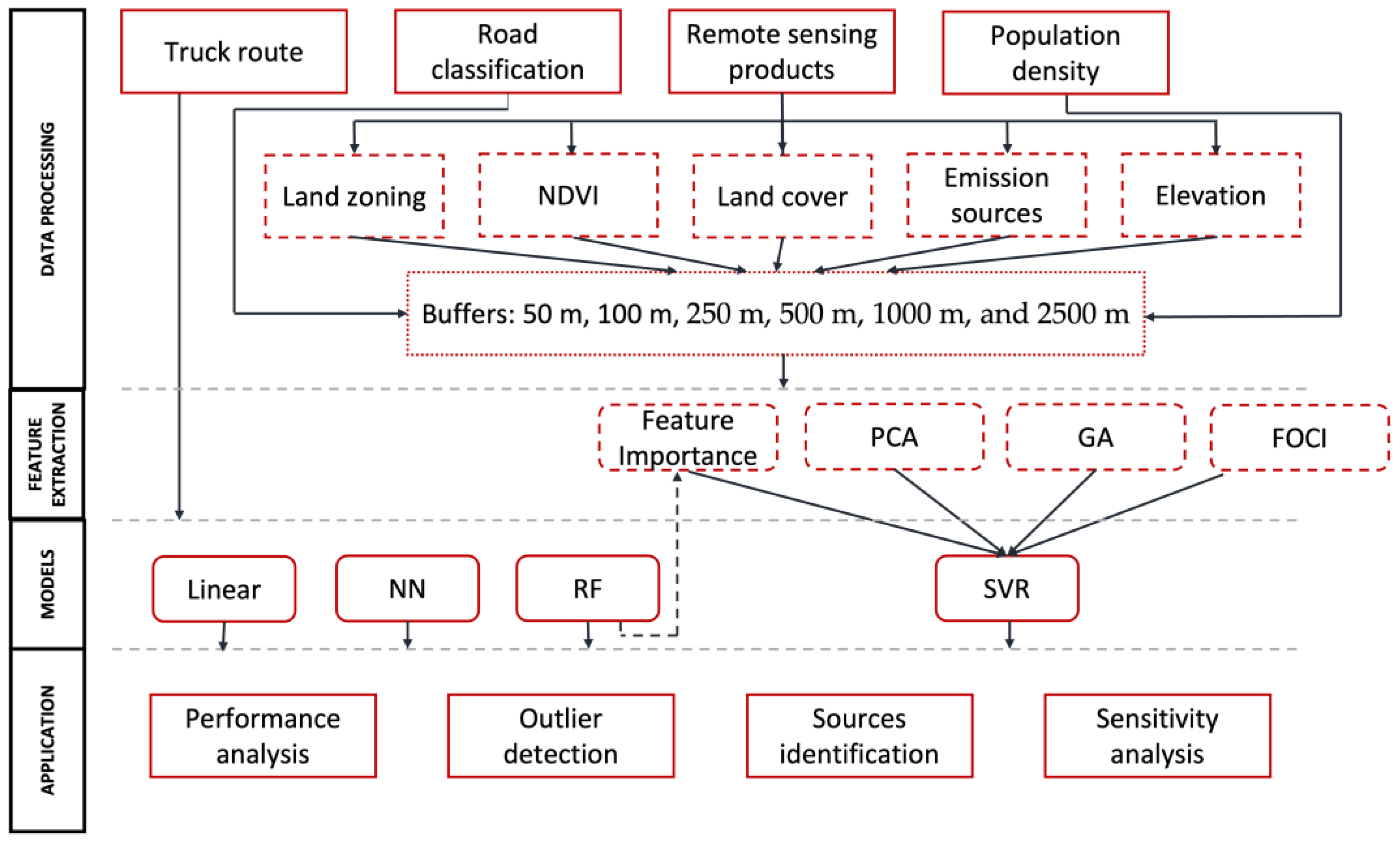
2.2. Land Use Model Specification

As mentioned, the primary challenge of our study is to effectively utilize LUR models with extensive, spatially detailed data. In this situation, we have over 5500 sections of 30 m roadways, each with an annual average BC concentration. To fully benefit from the spatial resolution provided by these concentrations, it is essential to have land use variables that ideally vary at or close to the same spatial scale. For defining the LUR, we employ the natural logarithm of BC concentrations as the dependent variable, as the distribution of log-transformed BC concentrations more closely resembles a normal distribution. Following the approach outlined by Messier et al. (2018) [38], we compute independent variables incorporating factors such as road length, road classifications, truck routes, local zoning categories, normalized difference vegetation index, land cover, population, point sources, elevation, and more (refer to Section S1 in supplementary material). Six buffer sizes (50 m, 100 m, 250 m, 500 m, 1000 m, and 2500 m) were used to calculate 108 variables. Before performing regression analysis, we normalized numeric variables to have a mean of zero and unit variance.

2.3. Model Specification

Four machine learning models are developed to analyze the processed land use variables. These are a linear model; random forest (RF); support vector regression (SVR); and neural network (NN). Our models are constructed using Python 3.7.6 [39] and scikit-learn 0.22 [40]. For the linear model, the least absolute shrinkage and selection operator (LASSO) algorithm is applied for both feature selection and regression. We regularize independent variable coefficients with a shrinkage parameter to limit their magnitude, which helps prevent overfitting and identifies influential features. The LASSO model also serves as a benchmark for comparison with other models.
RF utilizes resampling techniques to create numerous regression trees; this constitutes a supervised learning algorithm. The individual trees function as an ensemble, with key features emerging in the final model’s aggregation. The RF model is a versatile and robust model which is capable of handling complex data.
SVR is a machine learning model that utilizes support vector machines for regression tasks. It aims to find an optimal hyper-plane that maximizes the margin between predicted and actual target values. SVR applies kernel functions to map nonlinear data into a high-dimensional feature space where complex nonlinear relationships become linear. The dependent variables are regressed against the independent variable via the optimization of the support vectors. SVR is sensitive to input features and requires meticulous feature selection. Three feature selection methods and one dimension reduction method are applied to pre-process the input features to optimize SVR performance; these are random forest feature importance ordering, feature ordering by conditional independence (FOCI), the genetic algorithm (GA), and principal component analysis (PCA). Section 2.4 explains these feature pre-processing algorithms.
NN is a powerful deep learning model which is inspired by the structure and function of the human brain. It consists of many inter-connected layers or artificial neurons which can learn complex, nonlinear patterns. A multi-layer feed-forward neural network model is developed in this study to predict BC concentrations based on land use variables. A graphics processing unit (GPU) is used to increase the training process of the NN model, and all the work is carried out in the Google Colaboratory Cloud platform [41].

2.4. Model Tuning

Tuning refers to the optimization of a machine learning (ML) model by selecting suitable hyperparameters that guide the learning process.
We need to employ different methods for specifying the hyperparameters for our models. The grid search algorithm is used to optimize the constant shrinkage parameter of the LASSO model. For the RF model, multiple hyperparameters need to be tuned, which can be computationally demanding. We integrate RF with the Bayesian hyperparameter optimization algorithm, a probabilistic model-based technique. This method uses previous iterations’ information to build a probability model, which increases search efficiency. The actual objective function’s hyperparameters are optimized according to this probability model. We utilize Hyperopt [42] to carry out the Bayesian hyperparameter optimization procedure. The detailed tuning process with the Hyperopt optimization algorithm is illustrated in Figure S1 in the supplementary material. We define the search space for the RF hyperparameters (Table S1), and the optimization function within Hyperopt yields the optimized values for all hyperparameters (Table S2). For consistency, we set the maximum iteration numbers to 100 for all Bayesian hyperparameter optimization processes.
FOCI calculates conditional dependence coefficients based on the predictive power to select a subset of input features, which is a forward stepwise feature selection method [43]. The RF model uses regression trees to make predictions, which can also calculate the relative importance of each input feature. Based on this relative feature importance, we can subset different numbers of features as input for the SVR model. The GA-based method is uniquely designed to select optimized feature combinations and SVR model hyper-parameters, concurrently [44].
Utilizing the FOCI method, we selected 13 features from the 108 input features (Table S3), which are used as input variables for the SVR model. The SVR model is then tuned by the Bayesian optimization algorithm. Similarly, different feature combinations are selected by the RF feature importance and PCA methods, and the corresponding SVR models are optimized by the Bayesian optimization algorithm.
The fittest survival strategy with the next generation of offspring is introduced into the optimization process to create the genetic algorithm (GA). In this algorithm, the solution of each iteration is represented by a “chromosome”, which represents a set of parameters (features and hyperparameters in this case). The fitness value (R2) is calculated for every individual to indicate the solution’s quality. We initialize the GA algorithm by randomly creating 100 individuals to form a mating pool. Two individuals with the highest fitness values are chosen as parents, and they will produce eight offspring. The newly generated offspring and the parents together form an updated mating pool, which iterates until the fitness value does not improve or the number of iterations matches its maximum threshold. Mutation and crossover are applied to the mating process to introduce randomness to avoid the algorithm getting stuck at the local optimum points. The setup of the GA method’s parameters is listed in Section S3.2, and more details about this algorithm are described in Zhang et al.’s work [44].
Lastly, we manually adjust the NN model to achieve good prediction performance while preventing overfitting. The number of layers, the number of neurons in each layer, and the activation functions are carefully tuned with experience. Ultimately, the model with the highest prediction accuracy is selected.

2.5. Model Validation

The data are randomly split into training and validation sets, which account for 80% and 20% of the total number of samples, respectively. To split the data into training and validation sets, we first randomly shuffled the data to ensure that the split is representative and avoid any potential bias that might exist in the original order of the data. The next step is to split the data based on the split ratio, which in our case is 80% of the data split into the train set and 20% into the validation set. As for the 80% and 20% split ratio, it is the most widely used ratio in various fields and has proven to be effective in many scenarios. In our case, this split ratio provides enough data to train the models, allowing them to learn complex relations, and allocates a substantial amount of data to evaluate the models’ performance accurately. During the tuning process of all the models, only the train set is used (Section 2.4), while the validation data are employed to calculate the coefficient of regression (R2) and root mean square error (RMSE) for each optimized model. These metrics serve as the criteria for evaluating each model’s performance. For consistency, we use R2 as the criterion to fine-tune all models over the training set, and 5-fold cross-validation is implemented to calculate R2 to prevent overfitting.

3. Results

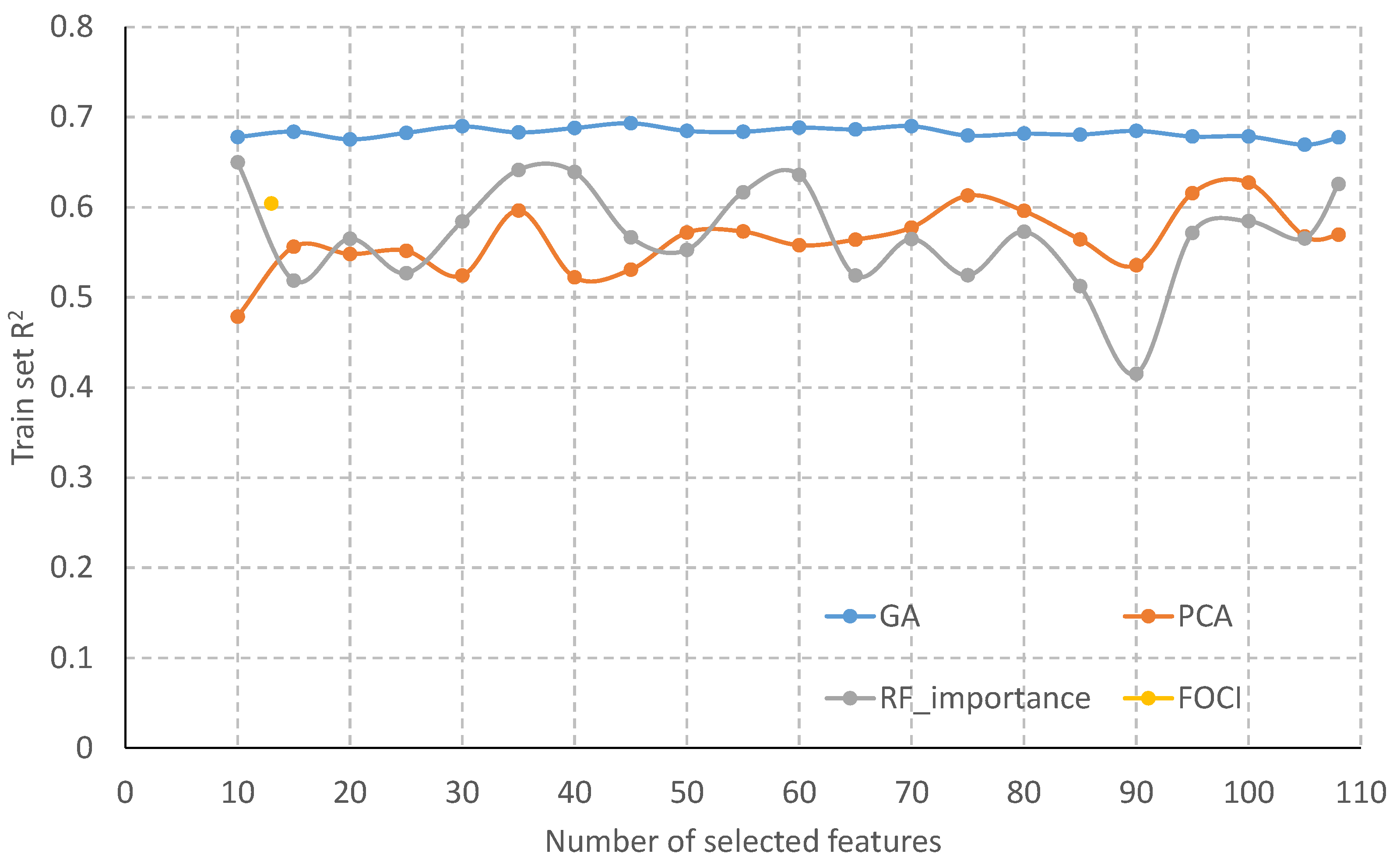
3.1. Model Development

A total of 75 features are selected by the LASSO model, and Table S6 lists the corresponding regression coefficients. The train and validation set R2s of the LASSO model are 0.596 and 0.594, respectively. The very similar R2s show the accuracy and robustness of the LASSO model in predicting BC concentrations.
For the RF model, Table S2 shows the optimized hyper-parameter values. The train and validation set R2s based on the RF model are 0.701 and 0.695, respectively. Like the LASSO model, RF also shows robustness when coupled with land use models in air pollution predictions.
Since the SVR model is sensitive to feature collinearity, it is necessary to conduct feature selection or dimension reduction to achieve better performance. SVR models with a different number of features as input are trained, and the train set R2s are shown in Figure 3. The GA method provides the best performance of all the pre-processing methods used for SVR model optimization, which selects 45 feature combinations with R2 of 0.693 and 0.667 for the train and validation sets, respectively. Tables S4 and S5 list the optimized hyper-parameters of the SVR model and the 45 selected features. The difference between train and validation set R2s proves that the SVR model is less robust and less generalizable than LASSO and RF.
The NN model shows R2s of 0.723 and 0.467 for train and validation sets, respectively; it has the highest train set R2s and lowest validation set R2s among all models in this study. The large difference between train and validation set R2s suggests that the NN model may have overfitting issues. The NN model contains three dense layers with a sigmoid as an activation function for all layers. There are 50, 25, and 10 neurons in each layer, respectively.
The R2s and RMSEs of each model over the train and validation sets are summarized in Table 1 below. The RMSEs agree relatively well with the R2s; RF has the lowest RMSE value, followed by SVR, but NN has a smaller RMSE value than LASSO, although LASSO has a higher validation R2 than NN.

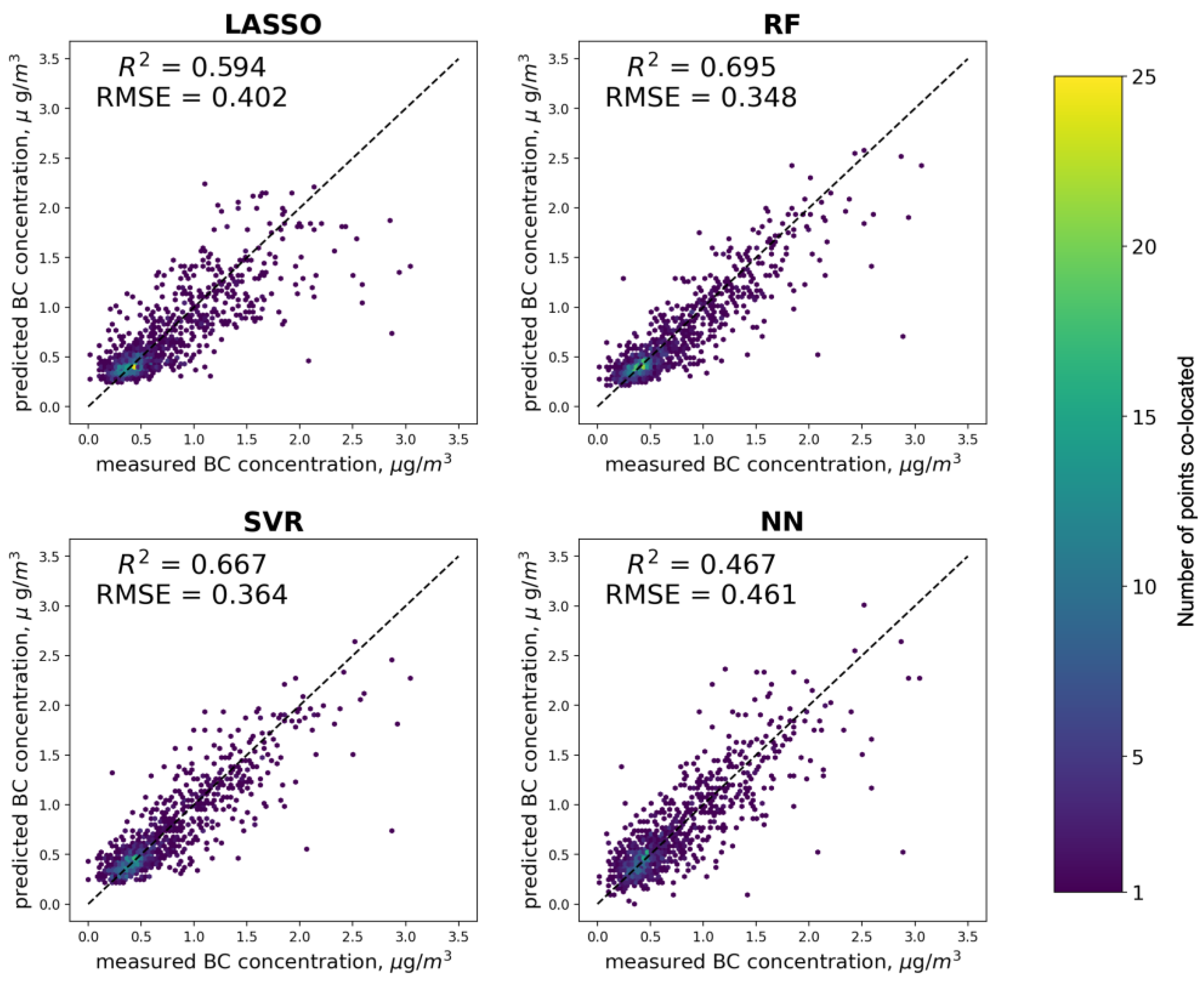
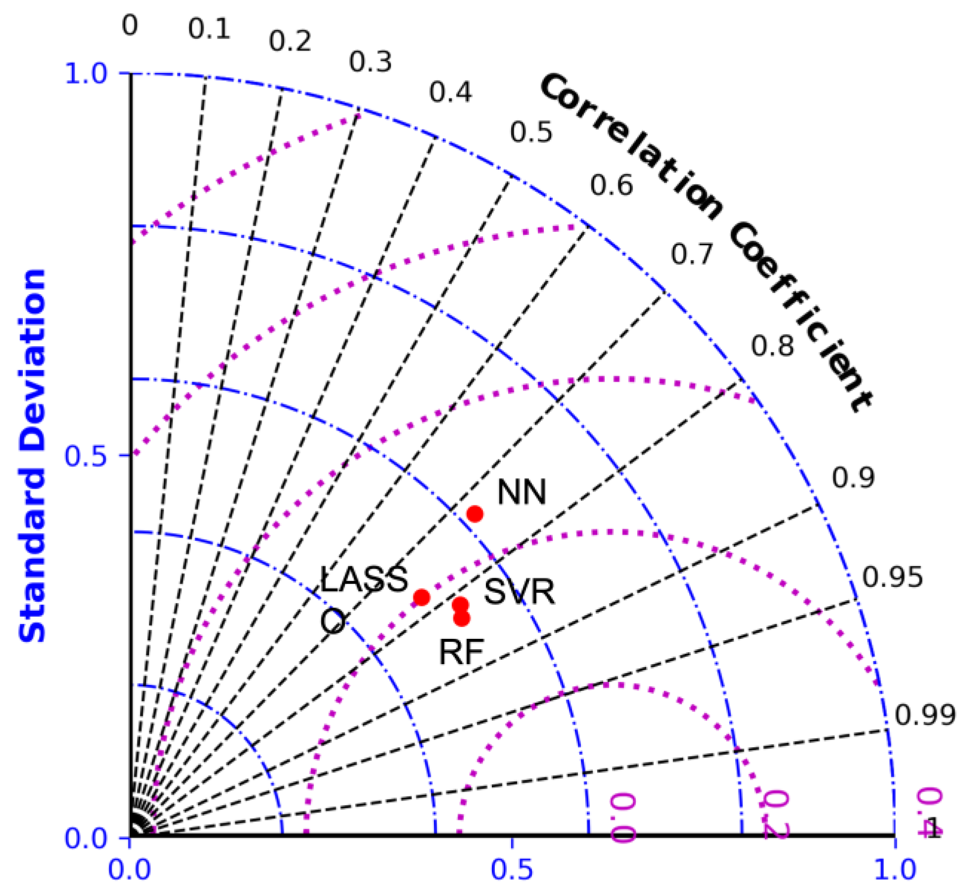
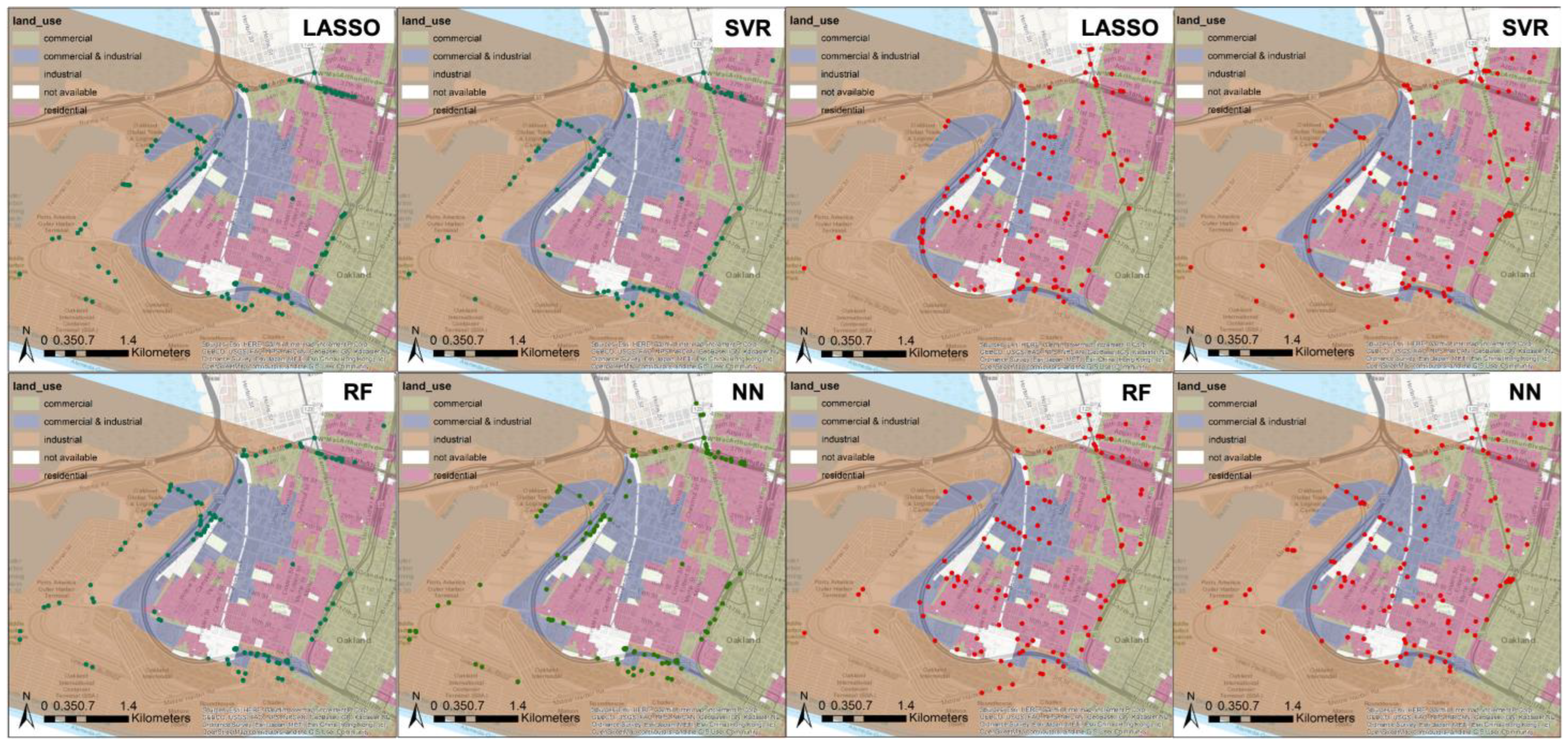
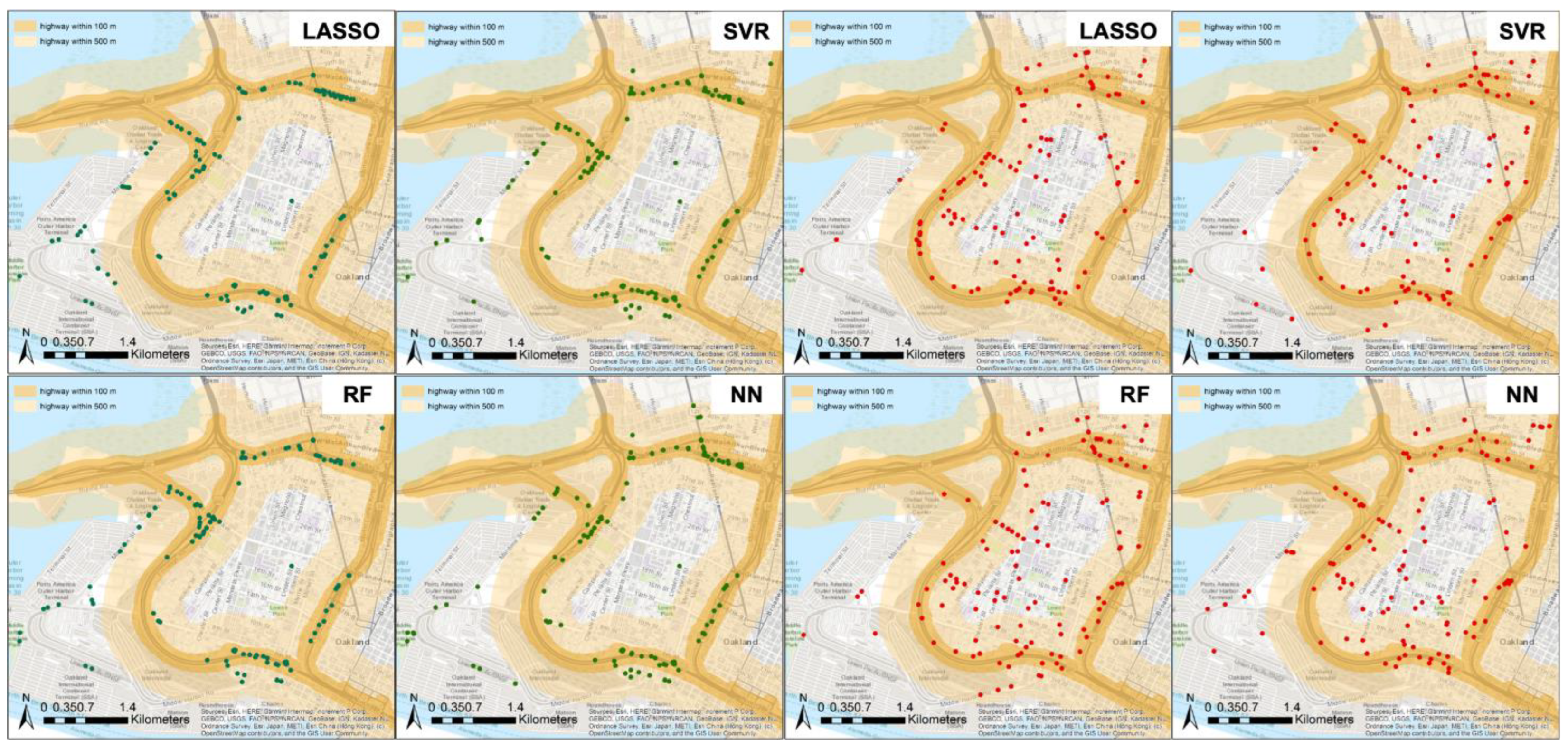
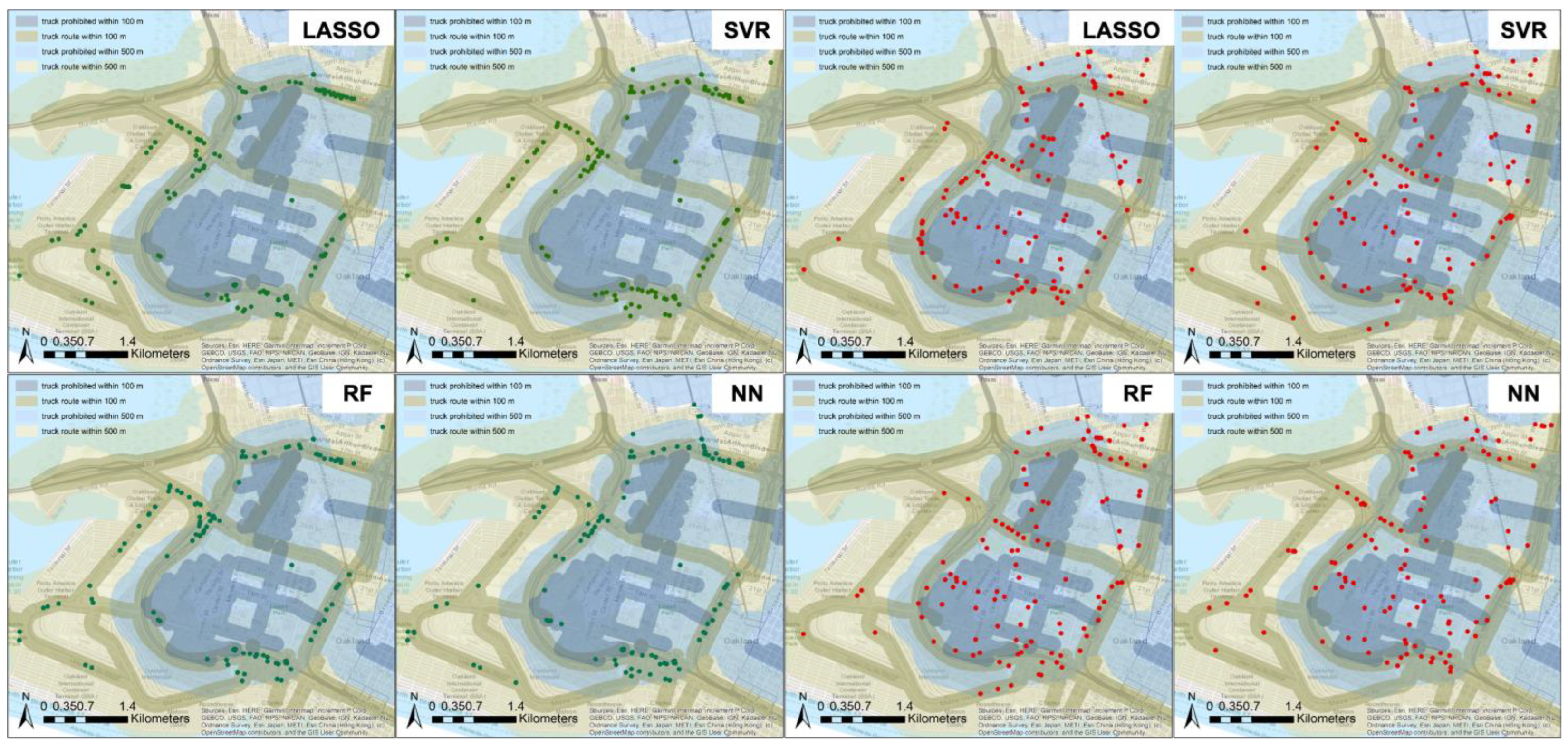
3.2. Model Performance Evaluation

RF has the best performance among all the models, with the highest R2 and lowest RMSE over the validation set. The scatter plots comparing model predicted values against measured values in the validation set are shown in Figure 4. All the models do not show significant bias in their predictions. The LASSO and NN models show more outliers and are more scattered than SVR and RF models, which are consistent with their R2 and RMSE performance. All four models have more outliers below the 1:1 line, suggesting they fail to capture some hyperlocal hotspots fully.
Figure 5 shows the Taylor diagram to compare the prediction performance of all four models. The Taylor diagram is a common method used to compare different models or datasets to reproduce observed data. The diagram consists of a polar plot, where each model is represented as a point in the figure. The Taylor diagram is based on statistical measurements including correlation, standard deviation, and root mean square difference. From the figure, RF performs best, while SVR achieves similar performance, and both are better than LASSO and NN.
To better show the spatial distribution of outliers within the domain, we calculate the differences between model predicted and measured values and compare the spatial distribution of differences with some critical land use variables in Figure 6, Figure 7 and Figure 8. The measured values are used to normalize the differences, where green dots represent points less than 10th percentiles, representing locations where the model underestimates BC concentrations; the red dots designate points greater than 90th percentiles, representing the locations where the model overestimates the observed BC concentrations. The summary statistics of BC concentration between model predicted and measured values are shown in Table 2.
Figure 6 compares the spatial distribution between the normalized differences and the land use types. Overestimations from all the models are spatially scattered, while most underestimations happen in three clustered locations for all four models. When spatially overlaying the outliers with the land use types, underestimations tend to happen in the industrial and mixture of commercial regions.
When comparing the spatial distribution of the outliers over the local highway systems (Figure 7), most of the underestimated outliers are located within a 100 m distance from major highways. Nearly all the underestimated outliers happen within a 500 m distance from major highways. However, there are no strong relations between the overestimated outliers and the local highway systems.
The truck route has been identified as a significant variable in BC predictions [45,46,47]. Figure 8 shows the spatial relationship between designated truck routes and the outliers for all the models. Like local highway systems, most underestimated outliers are located within a 100 m distance from truck routes, and all the underestimated outliers are located within a 500 m distance from truck routes. The overestimated outliers are more spatially scattered, and their distributions are not influenced by truck routes.
The spatial clustering of underestimated points (green points) suggests that these models cannot fully capture hyperlocal hotspots. In contrast, the distribution of overestimated points (red points) suggests that models’ overestimations happen relatively randomly.

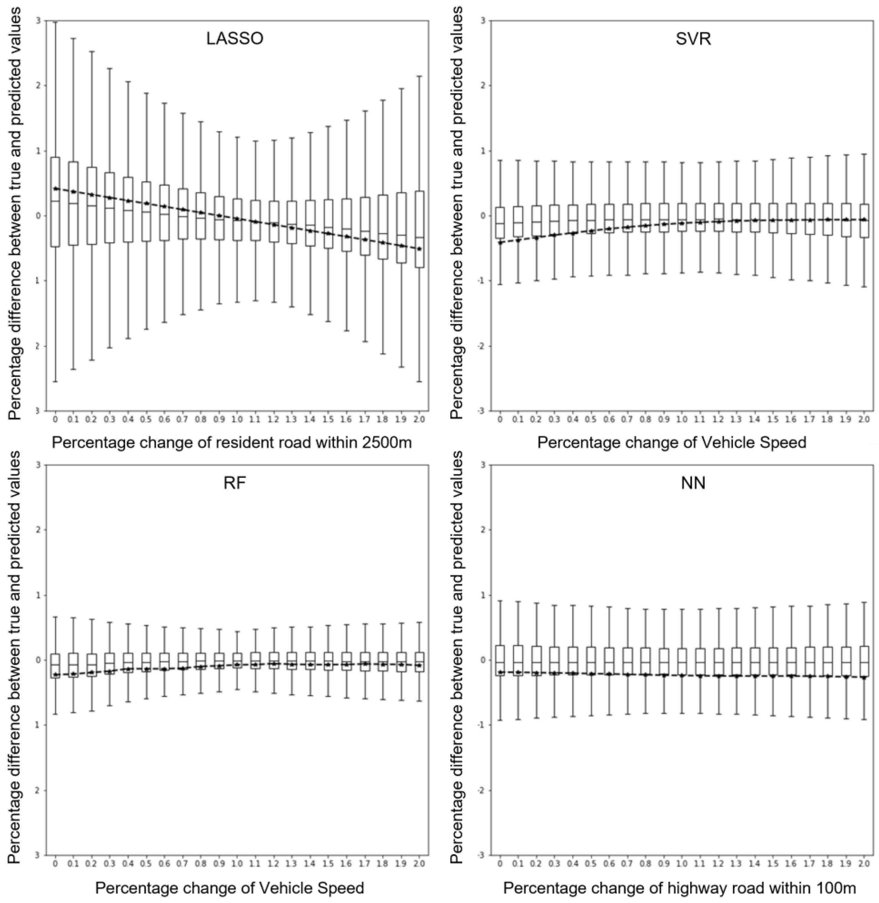
3.3. Sensitivity Analysis

The one-factor-at-a-time (OAT) method is utilized to analyze the relative importance of input features in influencing the models’ performance. As the name suggests, the OAT method perturbs one feature at a time from 0% to 200% with a 10% increment, while keeping the rest constant. The deviation of model predicted BC concentrations from the observed measurements is then determined. The most sensitivity features of all the models are plotted in Figure 9, which also illustrates how the varying input features influence BC concentration predictions. For SVR, RF, and NN models, the vehicle speed is highly sensitive in influencing the models’ performance; it is the most sensitive feature in both SVR and RF. The total length of the residential roads with the 2500 m distance and the total length of the highway with the 100 m distance is the most sensitive feature for LASSO and NN, respectively. Variables about local road networks including highways, arterials, and residential roads are dominant for the top five features that are highly influential to the models’ performance. Figure S2 lists detailed information about the top five most sensitive features of each model.
Among all four models, the RF model is the most robust; its prediction is most unlikely to be affected by the changing of a single input variable. On the other hand, the LASSO model shows the least robustness; its prediction is significantly influenced by the changing of input features. The sensitivity analysis indicates that traffic conditions (vehicle speed) and local road system (proximity and road type) are crucial for predicting BC concentrations for all models, which is a logical and expected result.

4. Discussion

This study shows that there are certain benefits when combining advanced machine learning methods with LUR models. However, some consistent underestimation patterns were observed with all the models, suggesting that they fail to fully capture hyperlocal hotspots in complex urban environments. The underestimation of BC concentrations from all four models is consistent; most of the underestimated points are spatially within three clusters, which are located within industrial and mixed commercial and industrial zoning areas, and within 100 m distance from major highways and truck routes. Conversely, there is no systematic bias of overestimations for all the models. For both underestimated and overestimated points, their locations from all four models do not exhibit any significant spatial pattern differences. These underestimation and overestimation patterns imply that the LUR model integrated with advanced machine learning algorithms and hyper-local air pollution measurements may still have difficulty fully capturing local hotspots, especially near complex emission sources, like major highways and truck routes.
Regarding the performance of the various models, LASSO is the simplest model with the shortest training time (only a few minutes to train and predict on a personal laptop); however, it can only capture linear relationships, leading to lower prediction accuracy than SVR and RF. The pre-processing that selects features or reduces input dimensions is crucial for optimizing the SVR model’s performance. The feature pre-processing and the SVR algorithm itself are computationally expensive. It costs over 500 iterations to optimize the 45 feature combinations and the SVR model hyper-parameters. Although the converging speed may be improved via the optimization of the GA method, the GA-based feature selection method still demands many iterations, making it computationally expensive (taking several hours or days on a personal laptop). The inherent suitability of parallel computing of the RF model makes it much faster in training (about one hour). The RF model’s robustness to input features’ collinearity helps it achieve better performance than the SVR model, without requiring any feature selection or dimension reduction processes, even though the latter model carefully selects the input features. This result suggests that the RF model is the best machine learning algorithm that could be coupled with the land use model in urban-scale air pollution prediction studies.
The NN model performs best over the training data but is the least accurate over the validation set among all the models. Adding an extra pre-processing step to select input features or reduce input dimension may improve the NN model’s overfitting issue and achieve better performance. Moreover, adding a dropout layer or early stopping technique to the NN model may also improve its performance [48,49]. However, the training process of NN is considerably slower than the other three models, even with the introduction of a GPU (taking about one hour for a single training and prediction process). The automatic NN structure selection algorithms are mostly based on iterations, which will take much longer time to optimize their structure. As a result of computational resource limitations, we do not conduct comprehensive feature pre-processing calculations and automatic structure optimization algorithms on the NN model. If optimizing prediction accuracy is the sole purpose of a study, it may be worth allocating the necessary computational resources to tuning the NN model with feature pre-processing steps and an automatic structure optimization algorithm. However, if there are other purposes besides predicting air pollution concentrations, e.g., health risk assessment, urban planning, etc., the RF model should be the first choice due to its high prediction accuracy, shorter training time, and robustness of using different features as input.
Our study achieves a reasonably good prediction accuracy in comparison to the existing literature. For instance, in Ghent, Belgium, Hover et al. used a mobile platform to measure BC concentrations in December 2015. They built the linear model coupling with the land use model, which achieved a cross-validation R2 of 0.520 [23]. Messier et al. used the same campaign data as our work but with a broader domain, including measurements from Downtown Oakland and East Oakland areas. They integrated kriging regression with the land use model, which provides a cross-validation R2 of 0.43 [38]. Our work exhibits better prediction accuracy than these studies with a more readily generalizable method.
Lim et al. provide similar prediction accuracy to our work, based on the mobile measurement of PM2.5 particle numbers in Seoul, Republic of Korea [50]. In their work, the stacked ensemble method exhibits better performance than our results, which is because this approach combines several machine learning models’ results to improve accuracy. But this model costs more computational resources to train and is difficult to generalize. Ren et al. coupled 13 machine learning models with the LUR model to analyze ozone data across the U.S. from over 1000 monitors and concluded that RF and extreme gradient boosting are the best-performing models [51], which is consistent with our results. Moreover, our work extends Ren et al.’s conclusion from the national scale to the hyper-local scale.
This study only focuses on a relatively small area and utilizes some specific independent variables (e.g., vehicle speed), making it difficult to generalize to more diverse regions. However, with the development of remote sensing products and geospatial techniques, it is possible to extract traffic conditions with deep learning methods over high-resolution satellite products and UAV images. The integration of traffic conditions and road speed limit can replace the vehicle speed variable in air pollution prediction and makes the model generalizable over larger and more diverse regions. The next step is to generalize the proposed LUR model over larger areas by utilizing remote sensing products and advanced geospatial techniques and exploring the potential application of predicted super-high-resolution BC concentration maps in environmental justice, environmental quality assessment, and health exposure studies.

5. Conclusions

This study develops land use regression models based on high-resolution mobile measured BC concentrations in West Oakland, CA, USA, integrating four machine learning models, including LASSO, SVR, RF, and NN. The models are carefully tuned on the training set, and the performance is evaluated on the validation set, which is independent of the training process. This work concludes that RF is the best-performing model for air pollution concentration prediction in epidemiology modeling, health exposure assessment, and urban planning studies. It is important to note that regardless of the regression algorithms used, the LUR model is less efficient at identifying localized hotspots, particularly when highways and truck routes are significant sources linked to local hotspots. This highlights the need for further research and development of models that can better capture hyperlocal variations in air pollution concentrations.

Supplementary Materials

The following supporting information can be downloaded at: https://www.mdpi.com/article/10.3390/ijgi12070290/s1, Figure S1: General procedure for using Hyperopt optimization algorithm to tune machine learning models (TPE is Tree of Parzen Estimators, which is a widely used optimization algorithm in Hyperopt algorithm). Figure S2. Top 5 most sensitive features for each model and how their variations influence model performance in BC prediction (box shows 25th, 50th, and 75th percentiles; dot means mean value).; Table S1. Search space for RF model hyper-parameters. Table S2. Tuned values of RF model hyper-parameters. Table S3. The FOCI method selected 13 features for the SVR model. Table S4. GA optimized hyper-parameters of the SVR model. Table S5. GA selected 45 features for the SVR model. Table S6. LASSO selected features and the coefficients.

Author Contributions

Conceptualization, Minmeng Tang and Deb A. Niemeier; methodology, Minmeng Tang; software, Minmeng Tang; validation, Minmeng Tang and Deb A. Niemeier; formal analysis, Minmeng Tang; investigation, Minmeng Tang; resources, Minmeng Tang and Deb A. Niemeier; data curation, Minmeng Tang; writing—original draft preparation, Minmeng Tang and Deb A. Niemeier; writing—review and editing, Minmeng Tang, Deb A. Niemeier and Tri Dev Acharya; visualization, Minmeng Tang; supervision, Deb A. Niemeier; project administration, Minmeng Tang and Deb A. Niemeier. All authors have read and agreed to the published version of the manuscript.

Funding

This research received no external funding. The APC was funded by the University of California Davis Open Access Fund (UCD-OAF).

Institutional Review Board Statement

Not applicable.

Data Availability Statement

Further inquiries can be directed to the corresponding author.

Conflicts of Interest

The authors declare no conflict of interest.

References

  1. Pinault, L.L.; Weichenthal, S.; Crouse, D.L.; Brauer, M.; Erickson, A.; Van Donkelaar, A.; Martin, R.V.; Hystad, P.; Chen, H.; Finès, P.; et al. Associations between Fine Particulate Matter and Mortality in the 2001 Canadian Census Health and Environment Cohort. Environ. Res. 2017, 159, 406–415. [Google Scholar] [CrossRef]
  2. Lu, X.; Lin, C.; Li, W.; Chen, Y.; Huang, Y.; Fung, J.C.H.; Lau, A.K.H. Analysis of the Adverse Health Effects of PM2.5 from 2001 to 2017 in China and the Role of Urbanization in Aggravating the Health Burden. Sci. Total Environ. 2019, 652, 683–695. [Google Scholar] [CrossRef]
  3. Lin, H.; Tao, J.; Du, Y.; Liu, T.; Qian, Z.; Tian, L.; Di, Q.; Rutherford, S.; Guo, L.; Zeng, W.; et al. Particle Size and Chemical Constituents of Ambient Particulate Pollution Associated with Cardiovascular Mortality in Guangzhou, China. Environ. Pollut. 2016, 208, 758–766. [Google Scholar] [CrossRef]
  4. Yang, J.; Zhou, M.; Li, M.; Yin, P.; Hu, J.; Zhang, C.; Wang, H.; Liu, Q.; Wang, B. Fine Particulate Matter Constituents and Cause-Specific Mortality in China: A Nationwide Modelling Study. Environ. Int. 2020, 143, 105927. [Google Scholar] [CrossRef]
  5. Crouse, D.L.; Philip, S.; Van Donkelaar, A.; Martin, R.V.; Jessiman, B.; Peters, P.A.; Weichenthal, S.; Brook, J.R.; Hubbell, B.; Burnett, R.T. A New Method to Jointly Estimate the Mortality Risk of Long-Term Exposure to Fine Particulate Matter and Its Components. Sci. Rep. 2016, 6, 18916. [Google Scholar] [CrossRef] [Green Version]
  6. Yang, J.; Sakhvidi, M.J.Z.; de Hoogh, K.; Vienneau, D.; Siemiatyck, J.; Zins, M.; Goldberg, M.; Chen, J.; Lequy, E.; Jacquemin, B. Long-Term Exposure to Black Carbon and Mortality: A 28-Year Follow-up of the GAZEL Cohort. Environ. Int. 2021, 157, 106805. [Google Scholar] [CrossRef]
  7. Wang, Y.; Pang, Y.; Huang, J.; Bi, L.; Che, H.; Zhang, X.; Li, W. Constructing Shapes and Mixing Structures of Black Carbon Particles with Applications to Optical Calculations. J. Geophys. Res. Atmos. 2021, 126, e2021JD034620. [Google Scholar] [CrossRef]
  8. Bond, T.C.; Doherty, S.J.; Fahey, D.W.; Forster, P.M.; Berntsen, T.; Deangelo, B.J.; Flanner, M.G.; Ghan, S.; Kärcher, B.; Koch, D.; et al. Bounding the Role of Black Carbon in the Climate System: A Scientific Assessment. J. Geophys. Res. Atmos. 2013, 118, 5380–5552. [Google Scholar] [CrossRef]
  9. Li, W.; Cao, Y.; Li, R.; Ma, X.; Chen, J.; Wu, Z.; Xu, Q. The Spatial Variation in the Effects of Air Pollution on Cardiovascular Mortality in Beijing, China. J. Expo. Sci. Environ. Epidemiol. 2018, 28, 297. [Google Scholar] [CrossRef] [PubMed]
  10. Moosmüller, H.; Chakrabarty, R.K.; Arnott, W.P. Aerosol Light Absorption and Its Measurement: A Review. J. Quant. Spectrosc. Radiat. Transf. 2009, 110, 844–878. [Google Scholar] [CrossRef]
  11. Tao, S.; Xu, H.; Ren, Y.; Zhang, W.; Meng, W.; Yun, X.; Yu, X.; Li, J.; Zhang, Y.; Shen, G.; et al. Updated Global Black Carbon Emissions from 1960 to 2017: Improvements, Trends, and Drivers. Environ. Sci. Technol. 2021, 55, 7869–7879. [Google Scholar] [CrossRef]
  12. Apte, J.S.; Messier, K.P.; Gani, S.; Brauer, M.; Kirchstetter, T.W.; Lunden, M.M.; Marshall, J.D.; Portier, C.J.; Vermeulen, R.C.H.; Hamburg, S.P. High-Resolution Air Pollution Mapping with Google Street View Cars: Exploiting Big Data. Environ. Sci. Technol. 2017, 51, 6999–7008. [Google Scholar] [CrossRef] [PubMed]
  13. Wang, A.; Xu, J.; Tu, R.; Saleh, M.; Hatzopoulou, M. Potential of Machine Learning for Prediction of Traffic Related Air Pollution. Transp. Res. Part D Transp. Environ. 2020, 88, 102599. [Google Scholar] [CrossRef]
  14. Xie, X.; Semanjski, I.; Gautama, S.; Tsiligianni, E.; Deligiannis, N.; Rajan, R.; Pasveer, F.; Philips, W. A Review of Urban Air Pollution Monitoring and Exposure Assessment Methods. ISPRS Int. J. Geo-Inf. 2017, 6, 389. [Google Scholar] [CrossRef] [Green Version]
  15. Farrell, W.J.; Weichenthal, S.; Goldberg, M.; Hatzopoulou, M. Evaluating Air Pollution Exposures across Cycling Infrastructure Types: Implications for Facility Design. J. Transp. L Use 2015, 8, 3. [Google Scholar] [CrossRef] [Green Version]
  16. Good, N.; Mölter, A.; Ackerson, C.; Bachand, A.; Carpenter, T.; Clark, M.L.; Fedak, K.M.; Kayne, A.; Koehler, K.; Moore, B.; et al. The Fort Collins Commuter Study: Impact of Route Type and Transport Mode on Personal Exposure to Multiple Air Pollutants. J. Expo. Sci. Environ. Epidemiol. 2015, 26, 397–404. [Google Scholar] [CrossRef]
  17. Krupnova, T.G.; Rakova, O.V.; Bondarenko, K.A.; Tretyakova, V.D. Environmental Justice and the Use of Artificial Intelligence in Urban Air Pollution Monitoring. Big Data Cogn. Comput. 2022, 6, 75. [Google Scholar] [CrossRef]
  18. Vu, T.; Shi, Z.; Cheng, J.; Zhang, Q.; He, K.; Wang, S.; Harrison, R. Assessing the Impact of Clean Air Action on Air Quality Trends in Beijing Using a Machine Learning Technique. Atmos. Chem. Phys. 2019, 19, 11303–11314. [Google Scholar] [CrossRef] [Green Version]
  19. Xu, L.; Zhang, J.; Sun, X.; Xu, S.; Shan, M.; Yuan, Q.; Liu, L.; Du, Z.; Liu, D.; Xu, D.; et al. Variation in Concentration and Sources of Black Carbon in a Megacity of China during the COVID-19 Pandemic. Geophys. Res. Lett. 2020, 47, e2020GL090444. [Google Scholar] [CrossRef]
  20. Reid, C.E.; Jerrett, M.; Petersen, M.L.; Pfister, G.G.; Morefield, P.E.; Tager, I.B.; Raffuse, S.M.; Balmes, J.R. Spatiotemporal Prediction of Fine Particulate Matter during the 2008 Northern California Wildfires Using Machine Learning. Environ. Sci. Technol. 2015, 49, 3887–3896. [Google Scholar] [CrossRef]
  21. Di, Q.; Kloog, I.; Koutrakis, P.; Lyapustin, A.; Wang, Y.; Schwartz, J. Assessing PM2.5 Exposures with High Spatiotemporal Resolution across the Continental United States. Environ. Sci. Technol. 2016, 50, 4712–4721. [Google Scholar] [CrossRef] [Green Version]
  22. Di, Q.; Amini, H.; Shi, L.; Kloog, I.; Silvern, R.; Kelly, J.; Sabath, M.B.; Choirat, C.; Koutrakis, P.; Lyapustin, A.; et al. An Ensemble-Based Model of PM2.5 Concentration across the Contiguous United States with High Spatiotemporal Resolution. Environ. Int. 2019, 130, 104909. [Google Scholar] [CrossRef]
  23. Van den Hove, A.; Verwaeren, J.; Van den Bossche, J.; Theunis, J.; De Baets, B. Development of a Land Use Regression Model for Black Carbon Using Mobile Monitoring Data and Its Application to Pollution-Avoiding Routing. Environ. Res. 2020, 183, 108619. [Google Scholar] [CrossRef] [Green Version]
  24. Talaat, H.; Xu, J.; Hatzopoulou, M.; Abdelgawad, H. Mobile Monitoring and Spatial Prediction of Black Carbon in Cairo, Egypt. Environ. Monit. Assess. 2021, 193, 587. [Google Scholar] [CrossRef]
  25. Kerckhoffs, J.; Hoek, G.; Messier, K.P.; Brunekreef, B.; Meliefste, K.; Klompmaker, J.O.; Vermeulen, R. Comparison of Ultrafine Particle and Black Carbon Concentration Predictions from a Mobile and Short-Term Stationary Land-Use Regression Model. Environ. Sci. Technol. 2016, 50, 12894–12902. [Google Scholar] [CrossRef]
  26. Alexeeff, S.E.; Roy, A.; Shan, J.; Liu, X.; Messier, K.; Apte, J.S.; Portier, C.; Sidney, S.; Van Den Eeden, S.K. High-Resolution Mapping of Traffic Related Air Pollution with Google Street View Cars and Incidence of Cardiovascular Events within Neighborhoods in Oakland, CA. Environ. Heal A Glob. Access Sci. Source 2018, 17, 38. [Google Scholar] [CrossRef] [Green Version]
  27. Hasenfratz, D.; Saukh, O.; Walser, C.; Hueglin, C.; Fierz, M.; Arn, T.; Beutel, J.; Thiele, L. Deriving High-Resolution Urban Air Pollution Maps Using Mobile Sensor Nodes. Pervasive Mob. Comput. 2015, 16, 268–285. [Google Scholar] [CrossRef]
  28. Weichenthal, S.; Ryswyk, K.; Goldstein, A.; Bagg, S.; Shekkarizfard, M.; Hatzopoulou, M. A Land Use Regression Model for Ambient Ultrafine Particles in Montreal, Canada: A Comparison of Linear Regression and a Machine Learning Approach. Environ. Res. 2016, 146, 65–72. [Google Scholar] [CrossRef] [Green Version]
  29. Sabaliauskas, K.; Jeong, C.H.; Yao, X.; Reali, C.; Sun, T.; Evans, G.J. Development of a Land-Use Regression Model for Ultrafine Particles in Toronto, Canada. Atmos. Environ. 2015, 110, 84–92. [Google Scholar] [CrossRef]
  30. Bao, F.; Cheng, T.; Li, Y.; Gu, X.; Guo, H.; Wu, Y.; Wang, Y.; Gao, J. Retrieval of Black Carbon Aerosol Surface Concentration Using Satellite Remote Sensing Observations. Remote Sens. Environ. 2019, 226, 93–108. [Google Scholar] [CrossRef]
  31. Li, Y.; Yuan, S.; Fan, S.; Song, Y.; Wang, Z.; Yu, Z.; Yu, Q.; Liu, Y. Satellite Remote Sensing for Estimating PM 2.5 and Its Components. Curr. Pollut. Rep. 2021, 7, 72–87. [Google Scholar] [CrossRef]
  32. Van Donkelaar, A.; Martin, R.V.; Li, C.; Burnett, R.T. Regional Estimates of Chemical Composition of Fine Particulate Matter Using a Combined Geoscience-Statistical Method with Information from Satellites, Models, and Monitors. Environ. Sci. Technol. 2019, 53, 2595–2611. [Google Scholar] [CrossRef] [Green Version]
  33. Lin, C.; Lau, A.K.H.; Fung, J.C.H.; Lao, X.Q.; Li, Y.; Li, C. Assessing the Effect of the Long-Term Variations in Aerosol Characteristics on Satellite Remote Sensing of PM2.5 Using an Observation-Based Model. Environ. Sci. Technol. 2019, 53, 2990–3000. [Google Scholar] [CrossRef]
  34. Silveira, C.; Ferreira, J.; Tuccella, P.; Curci, G.; Miranda, A.I. Combined Effect of High-Resolution Land Cover and Grid Resolution on Surface NO2 Concentrations. Climate 2022, 10, 19. [Google Scholar] [CrossRef]
  35. Tan, Q.; Ling, J.; Hu, J.; Qin, X.; Hu, J. Vehicle Detection in High Resolution Satellite Remote Sensing Images Based on Deep Learning. IEEE Access 2020, 8, 153394–153402. [Google Scholar] [CrossRef]
  36. Feroz, S.; Abu Dabous, S. UAV-Based Remote Sensing Applications for Bridge Condition Assessment. Remote Sens. 2021, 13, 1809. [Google Scholar] [CrossRef]
  37. Google Oakland_201506-201605_GoogleAclimaAQ. Available online: www.google.com (accessed on 1 November 2020).
  38. Messier, K.P.; Chambliss, S.E.; Gani, S.; Alvarez, R.; Brauer, M.; Choi, J.J.; Hamburg, S.P.; Kerckhoffs, J.; LaFranchi, B.; Lunden, M.M.; et al. Mapping Air Pollution with Google Street View Cars: Efficient Approaches with Mobile Monitoring and Land Use Regression. Environ. Sci. Technol. 2018, 52, 12563–12572. [Google Scholar] [CrossRef] [Green Version]
  39. Van Rossum, G.; Drake, F.L., Jr. Python Tutorial; Centrum voor Wiskunde en Informatica: Amsterdam, The Netherlands, 1995. [Google Scholar]
  40. Pedregosa, F.; Varoquaux, G.; Gramfort, A.; Michel, V.; Thirion, B.; Grisel, O.; Blondel, M.; Prettenhofer, P.; Weiss, R.; Dubourg, V.; et al. Scikit-Learn: Machine Learning in {P}ython. J. Mach. Learn. Res. 2011, 12, 2825–2830. [Google Scholar]
  41. Bisong, E. Google Colaboratory BT—Building Machine Learning and Deep Learning Models on Google Cloud Platform: A Comprehensive Guide for Beginners; Bisong, E., Ed.; Apress: Berkeley, CA, USA, 2019; pp. 59–64. ISBN 978-1-4842-4470-8. [Google Scholar]
  42. Bergstra, J.; Yamins, D.; Cox, D. Making a Science of Model Search: Hyperparameter Optimization in Hundreds of Dimensions for Vision Architectures. In Proceedings of the International Conference on Machine Learning, PMLR, Atlanta, GA, USA, 16–21 June 2013; pp. 115–123. [Google Scholar]
  43. Azadkia, M.; Chatterjee, S. A Simple Measure of Conditional Dependence. Ann. Stat. 2019, 49, 3070–3102. [Google Scholar] [CrossRef]
  44. Zhang, D.; Xiao, J.; Zhou, N.; Zheng, M.; Luo, X.; Jiang, H.; Chen, K. A Genetic Algorithm Based Support Vector Machine Model for Blood-Brain Barrier Penetration Prediction. Biomed. Res. Int. 2015, 2015, 292683. [Google Scholar] [CrossRef] [Green Version]
  45. Westerdahl, D.; Fruin, S.; Sax, T.; Fine, P.M.; Sioutas, C. Mobile Platform Measurements of Ultrafine Particles and Associated Pollutant Concentrations on Freeways and Residential Streets in Los Angeles. Atmos. Environ. 2005, 39, 3597–3610. [Google Scholar] [CrossRef]
  46. Abernethy, R.C.; Allen, R.W.; McKendry, I.G.; Brauer, M. A Land Use Regression Model for Ultrafine Particles in Vancouver, Canada. Environ. Sci. Technol. 2013, 47, 5217–5225. [Google Scholar] [CrossRef] [PubMed] [Green Version]
  47. Larson, T.; Henderson, S.B.; Brauer, M. Mobile Monitoring of Particle Light Absorption Coefficient in an Urban Area as a Basis for Land Use Regression. Environ. Sci. Technol. 2009, 43, 4672–4678. [Google Scholar] [CrossRef] [PubMed]
  48. Srivastava, N.; Hinton, G.; Krizhevsky, A.; Sutskever, I.; Salakhutdinov, R. Dropout: A Simple Way to Prevent Neural Networks from Overfitting. J. Mach. Learn. Res. 2014, 15, 1929–1958. [Google Scholar]
  49. Srivastava, N. Improving Neural Networks with Dropout. Univ. Tor. 2013, 182, 7. [Google Scholar]
  50. Lim, C.C.; Kim, H.; Vilcassim, M.J.R.; Thurston, G.D.; Gordon, T.; Chen, L.C.; Lee, K.; Heimbinder, M.; Kim, S.Y. Mapping Urban Air Quality Using Mobile Sampling with Low-Cost Sensors and Machine Learning in Seoul, South Korea. Environ. Int. 2019, 131, 105022. [Google Scholar] [CrossRef]
  51. Ren, X.; Mi, Z.; Georgopoulos, P.G. Comparison of Machine Learning and Land Use Regression for Fine Scale Spatiotemporal Estimation of Ambient Air Pollution: Modeling Ozone Concentrations across the Contiguous United States. Environ. Int. 2020, 142, 105827. [Google Scholar] [CrossRef]
Figure 1. General research structure and workflow of the paper.
Ijgi 12 00290 g001
Figure 2. Study domain and high-resolution BC concentration map.
Ijgi 12 00290 g002
Figure 3. Train set R2s of the SVR model based on different feature selection and dimension reduction algorithms.
Ijgi 12 00290 g003
Figure 4. Scatter plots between model predicted and measured values for all models.
Ijgi 12 00290 g004
Figure 5. Taylor diagram for all four models.
Ijgi 12 00290 g005
Figure 6. Spatial distribution of the outliers of each model over the land use types within the study domain (green dots are points less than the 10th percentile, while red dots are points greater than the 90th percentile).
Ijgi 12 00290 g006
Figure 7. Spatial distribution of outliers of each model over the local highway systems (green dots are points less than the 10th percentile, while red dots are points greater than the 90th percentile).
Ijgi 12 00290 g007
Figure 8. Spatial distribution of outliers of each model over the local truck routes (green dots are points less than the 10th percentile, while red dots are points greater than the 90th percentile).
Ijgi 12 00290 g008
Figure 9. How the most sensitive feature influences each model’s performance (dot means mean value, and box shows 25th, 50th, and 75th percentiles).
Ijgi 12 00290 g009
Table 1. Model performance criteria summary.
5-Fold CV R2 for Train SetR2 for Validation SetRMSE for Validation Set, µg/m3
LASSO0.5960.5940.273
SVR0.6930.6670.221
RF0.7010.6950.210
NN0.7230.4670.253
Table 2. BC concentration difference between model predicted and measurement concentrations.
BC Concentration Differences, µg/m3
Outliers (<10th Percentile)InliersOutliers (>90th Percentile)
MeanStandard DeviationMeanStandard DeviationMeanStandard Deviation
LASSO−0.520.35−0.010.160.320.19
RF−0.380.29−0.020.130.240.14
SVR−0.400.290.000.130.280.17
NN−0.410.320.000.160.330.20
Disclaimer/Publisher’s Note: The statements, opinions and data contained in all publications are solely those of the individual author(s) and contributor(s) and not of MDPI and/or the editor(s). MDPI and/or the editor(s) disclaim responsibility for any injury to people or property resulting from any ideas, methods, instructions or products referred to in the content.

