1. Introduction
For a long time, calculating the shortest (or fastest) path between locations A and B has been the center of pedestrian navigation systems’ attention. Nonetheless, “alternative routing” suggests that distance (or travel time) is not the only factor affecting the pedestrian’s route choices [
1,
2]. Other preferences, such as accessibility, convenience, comfort, etc., could be involved in such decisions [
3]. The geometry properties of the shortest paths, including route curviness, the number of turns and intersections along roads, road gradients, sidewalk conditions (surface type, width, texture, etc.), and so on, might influence the route choice decision of particular types of pedestrians [
4,
5]. This is especially the case for people with limited mobility, like wheelchair users and older adults, experiencing major difficulties getting around urban environments. According to the data from the Centers for Disease Control and Prevention (CDC), about 31 million (11.1%) adults in the United States live with mobility impairments [
6]. Previous studies [
7,
8] have shown that a straighter route (i.e., a route with fewer turns and long straight roads between turns) having equal or even longer travel time might be far preferable to a tortuous route for such users because of the convenience it may provide.
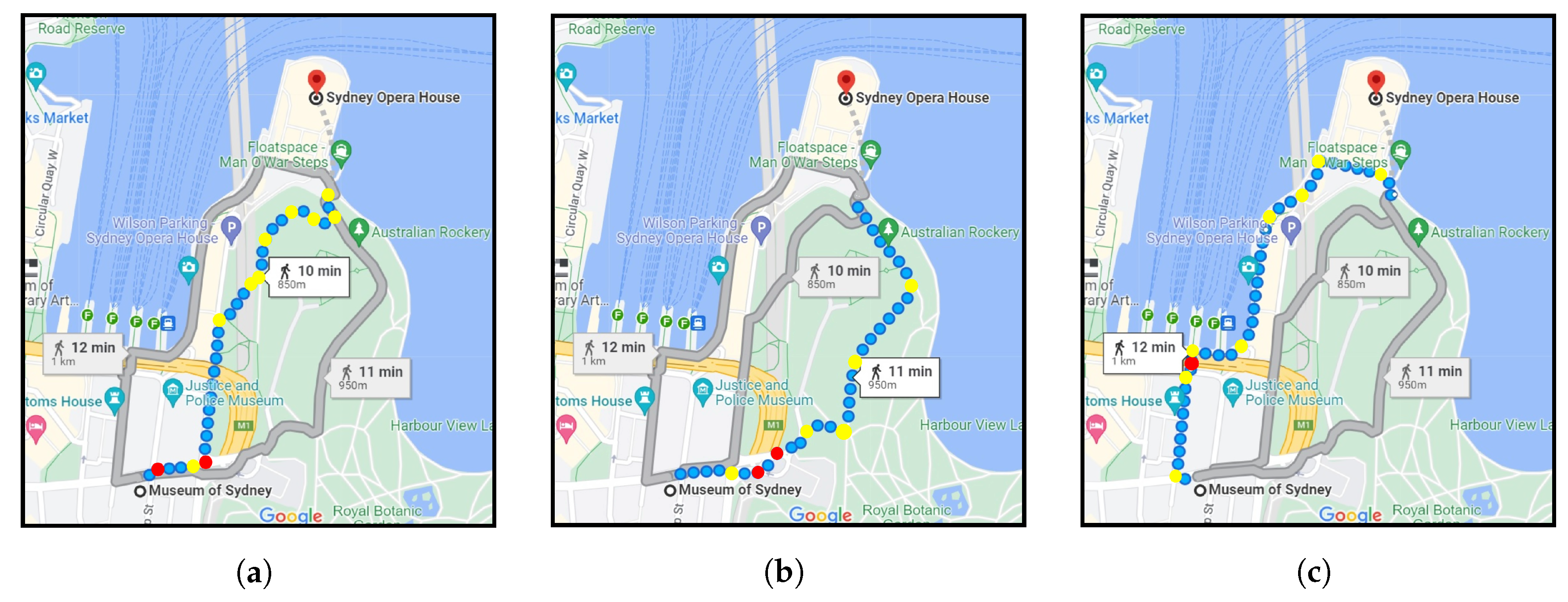
Figure 1 represents the shortest route (a) and alternative routes (b,c) between the “Museum of Sydney” and the “Sydney Opera House” suggested by Google Maps. It can be seen that despite showing small differences in the distance (850 m, 950 m, and 1 km) and travel time (10 min, 11 min, and 12 min), the routes have quite different geometric properties. In such situations, while many pedestrians generally ask “which path takes me to the destination faster?”, others might consider different factors that are directly or indirectly relevant to the geometry of the route as follows:
Which route shows the least curviness?
How many twists and turns (or directional changes) and intersections exist on each route?
Which route shows lower road gradients, making the walking experience more pleasant for pedestrians?
As a result, pedestrians could end up with different route choices depending on their individual preferences. For instance, an ordinary person is more likely to choose “route a”, given that it offers the shortest distance and travel time. Conversely, the possible choice of a wheelchair user might be “route b” as it shows lower average and maximum slopes on roads. On the other hand, an elderly person might choose “route c” as it has the least curviness, allowing the pedestrian to enjoy traversing longer straight streets between turns, thus, avoiding the inconvenience of passing multiple bends and junctions. Of course, the beautiful coastal scenery of “route c” could also be involved in such decisions, but they are out of the scope of this paper.
Pedestrian navigation is considered an area of interest that could significantly benefit from the OpenStreetMap (OSM), a successful crowdsourcing project providing a flexible way to gather and share geospatial data relevant to urban infrastructure and facilities. The OSM project has already received tremendous attention from the research community in urban planning and transportation. Graells-Garrido et al. (2021) [
9] used OSM to measure the accessibility to local urban amenities in Barcelona. Liu et al. (2021) [
10] proposed a method to quantify pedestrian accessibility at high resolution using open data, including OSM, Global Human Settlements Layer (GHSL), and General Transit Feed Specification (GTFS). Gil (2015) [
11] and Prieto-Curiel et al. (2022) [
12] applied OSM data for constructing multimodal and interurban network models, respectively. The San Francisco Bay Area’s road networks were extracted using OSM for traffic microsimulation at the metropolitan-scale [
13]. Yadav et al. (2021) [
14] chose OSM data to visualize traffic estimation results. Klinkhardt et al. (2021) [
15] extracted the places of interest (POIs) from OSM for estimating the attractiveness of traffic analysis zones (TAZs). Bartzokas-Tsiompras (2022) [
16] conducted a comparison study to analyze pedestrian street lengths in 992 cities worldwide. Moreover, there have recently been some efforts to investigate the fitness of OSM for route planning [
17], pedestrian navigation [
18,
19,
20,
21,
22], and navigation systems designed for disabled pedestrians [
23,
24,
25]. Furthermore, several methods and tools have been developed to assess and enrich OSM’s sidewalk information (width, surface texture, etc.) for pedestrian navigation and similar purposes [
25,
26,
27].
Road datasets owned by commercial mapping platforms (e.g., Google Maps, MapQuest, and ESRI) are not free to access, given that distributing such expensive data to the public might lead to the forfeiting of the company’s competitive advantage in offering web mapping services. Conversely, the OSM project could provide free, open access to a rich database of road data, particularly walkable roads (e.g., roads in residential areas, pedestrian-only streets, narrow roads, and alleyways), for developing navigation systems. Furthermore, while commercial mapping companies generally use a pay-as-you-go pricing model and require payment if you use their APIs for more than a certain amount, the OSM project is quite adaptable to the open-source model, which is important to those individuals and small businesses that cannot afford to buy such services. For instance, OpenRouteService (ORS), Open Source Routing Machine (OSRM), GraphHopper, and OpenTripPlanner (OTP) consume OSM data to offer route-planning services to users. Likewise, various specialized online map services, including bicycle maps, public transport maps, wheelchair user maps, and waymarked trails, rely on data from the OSM project.
To fulfill their tasks most efficiently, pedestrian navigation systems rely heavily on the quality and level of information they provide for users. The collaborative mapping nature of the OSM project could make it easier to gather and share the routing experience of pedestrians about the quality of sidewalks (straightness, surface, width, etc.) and any existent barriers or inconveniences on roads [
24]. There exist several crowdsourcing services, including CAP4Access [
28], OhsomeHex [
29], AXS Map [
30], and Project Sidewalk [
31], allowing volunteers to contribute their navigation experiences, such as surface conditions and obstacles along roads, to these services. Among these, the European CAP4Access is a successful OSM-centered project that develops methods and tools for pedestrians with limited mobility focusing on (a) quality assessment, (b) accessibility-level tagging of places, (c) route planning and navigation, and (d) raising awareness [
25].
Many authors have introduced factors relevant to the built environment affecting the walking behaviors of pedestrians [
32,
33,
34,
35]. Addressing the navigation needs of pedestrians, especially those with limited mobility, requires a clear understanding of their route choices and using them in developing navigation systems [
8]. Previous studies have demonstrated that besides distance, pedestrian route choice is connected to various other variables, including comfort [
36], safety [
37], attractiveness [
38], and route geometry [
4,
7,
39]. Focusing on route geometry, Kasemsuppakorn et al. (2015) [
8] suggested that navigation systems could be more helpful if they provide personalized routes based on individual preferences and physical characteristics of routes (i.e., surface condition and slope); while Jansen-Osmann and Wiedenbauer (2004) [
39] indicated that pedestrians perceive curvy routes to be longer than straight routes, a study by D’Acci (2019) [
4] flatly contradicted their claims. Using a discrete choice model on over 10,000 GPS trajectory data of pedestrians in two US cities, San Francisco and Boston, Sevtsuk and Basu (2022) [
7] found out that the effect of road turns on pedestrian route choice relies on network geometry. Another study listed distance and road turns as the main route choice criteria for pedestrians in Boston [
40]. Shatu et al. (2019) [
41] showed that distance and road turns contributed to over half of pedestrian route choices, but the latter is more important to pedestrians. Furthermore, pedestrian fatalities and injuries when crossing road intersections have been listed as a significant safety concern worldwide [
42]. Lastly, some studies have indicated the major impact of road gradients on walking attractiveness [
43,
44].
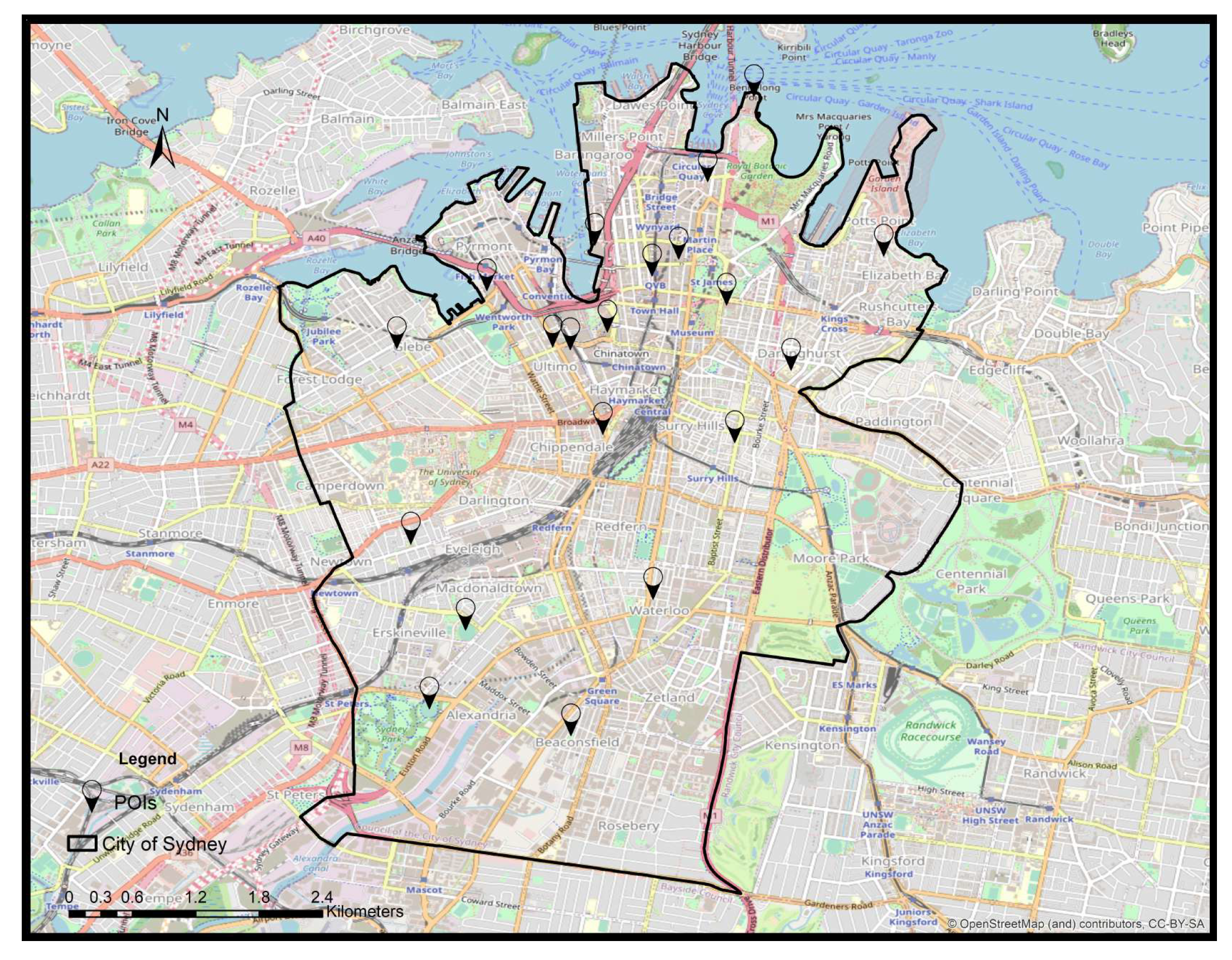
Even though the above studies have highlighted the significance of geometry information related to the route in pedestrian navigation, research has yet to be conducted in practice. Therefore, this study proposes new methodologies for extracting and analyzing the geometry properties of pedestrian shortest paths for navigation applications, focusing on open geospatial data. The analysis is carried out on free, open OSM road networks and elevation data, which are expected to be crucial in providing future data for pedestrian navigation services. A shortest path analysis is conducted on an origin–destination (OD) database within the City of Sydney, a local government area of Greater Sydney in Australia. The “OSRM”, as an OSM-based routing engine, and “Google Maps Directions API” are employed to implement the shortest path analysis. Then, the routes’ geometry characteristics are extracted by the devised measures in this study, and the results are analyzed comprehensively.
The remainder of this article is organized as follows: The methods and materials are introduced in the next section. In
Section 3, the results are presented with figures, tables, and relevant interpretations.
Section 4 discusses the results in the greatest detail possible. Lastly,
Section 5 summarizes the major findings and conclusions.
3. Results
The shortest path analysis between 20 × 20 OD pairs resulted in 380 route pairs (OSM and Google Maps) that were used for the geometry analysis. The results were categorized in distance matrices, and their geometry information was extracted accordingly.
Table 3 displays the overall distance and travel time statistics estimated for OSM and Google Maps. It indicates that, on average, OSM resulted in longer routes (1162 km) than Google Maps (1115 km). Likewise, OSM routes achieved longer travel times, an overall of 242 h 12 m against 232 h 28 m for Google Maps routes. Slight variations in distance estimates are normal. Even assuming a similar route pair suggested by two different commercial routing platforms, such as Google Maps and Mapbox, there might still be some differences in distance estimates due to the characteristics of road datasets, utilized algorithms, and other contributing factors.
Table 4 summarizes the comparative analysis of distance estimates in two separate sections: OSM routes (a) shorter and (b) longer than Google Maps; while about two-thirds of OSM routes were found to be longer than Google Maps, the magnitude of differences was moderate between 0 and 850 m. The average differences for OSM shorter and longer routes than Google Maps consecutively were −116 m and 201 m, indicating that OSM witnessed higher variations in the latter case. In addition, the deviation of OSM from Google Maps was concentrated in a range of −2.9–−12.5% and 2.1–14.5% for OSM shorter and longer routes, respectively. The paired-samples
t-test indicate a statistically significant difference between the mean distance estimates of OSM (M = 3.3, SD = 1.6) and Google Maps (M = 3.1, SD = 1.5),
= 7.4,
p < 0.001. Moreover, the distance average of Google Maps was smaller than OSM.
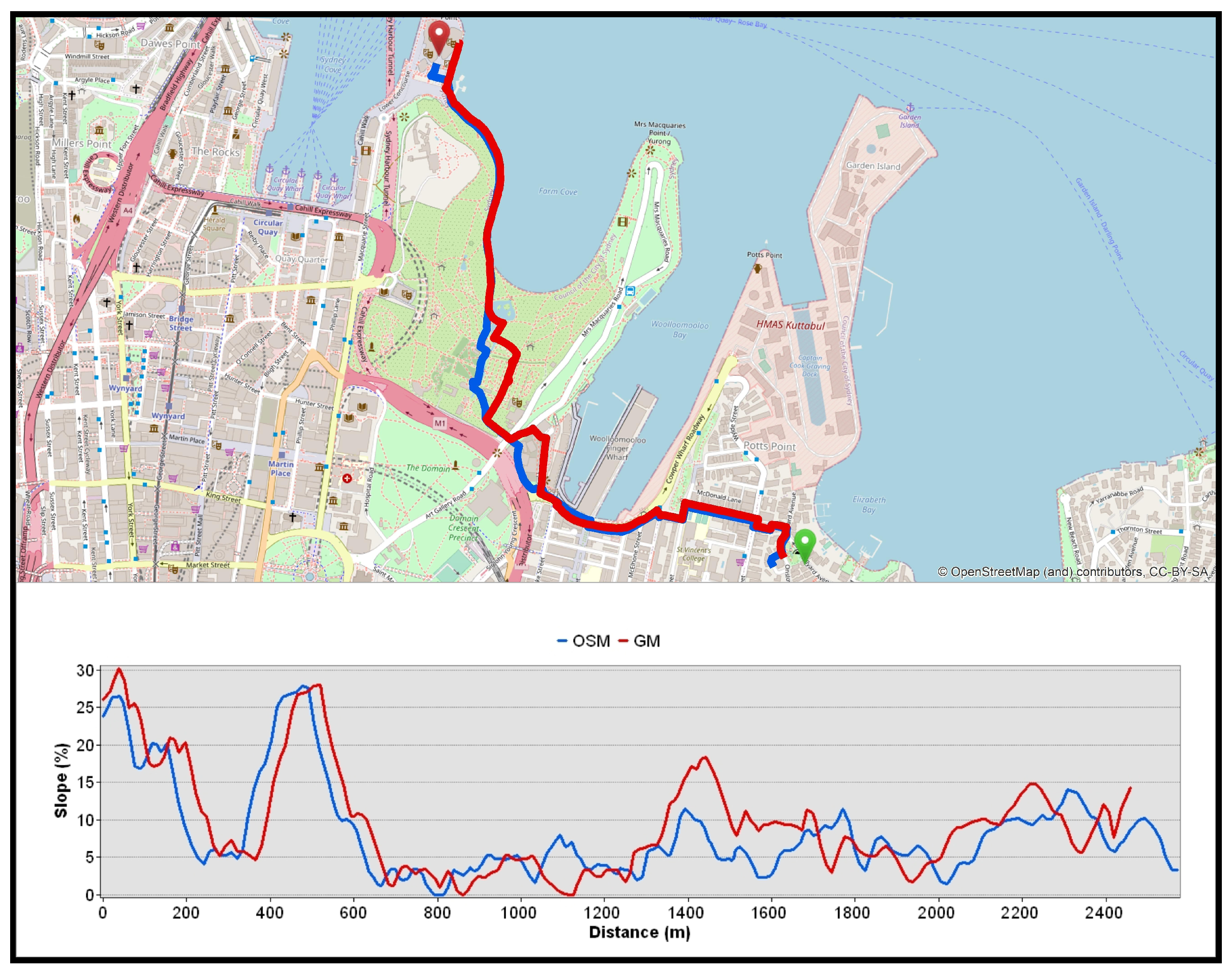
Figure 7 presents the calculated shortest paths with road slope profiles between “Elizabeth Bay House” and “Sydney Opera House” locations. According to
Table 5, OSM and Google Maps routes were remarkably similar in geometry, with a dissimilarity ratio of about 4%. The remaining statistics shown in
Table 6 indicate that the OSM route offers more comfort, convenience, and safety than Google Maps, given that it is less tortuous and pedestrians can expect smoother motion and better accessibility due to its lower average and maximum slopes.
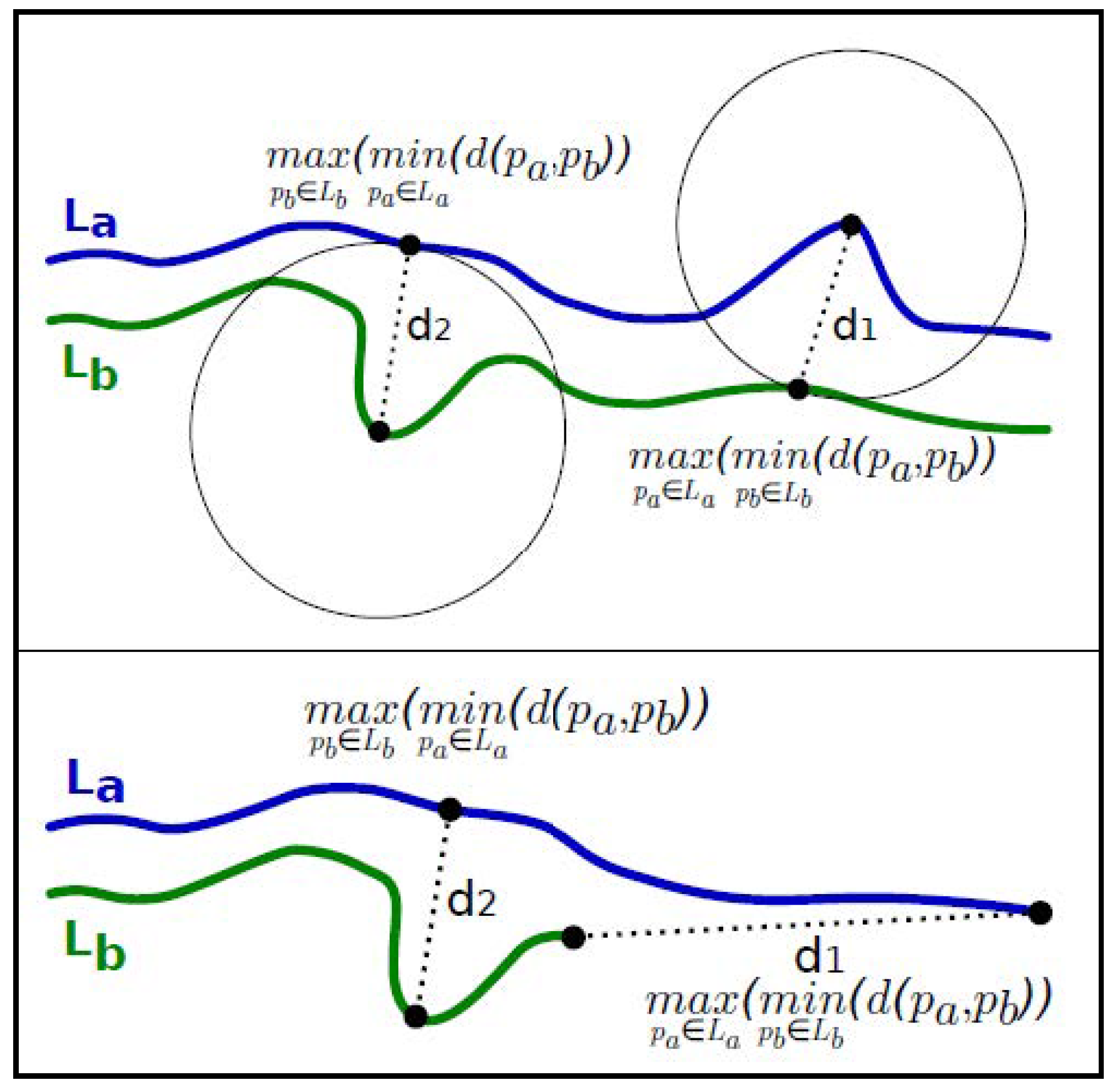
Achieving Hausdorff distances between 19 m and 1116 m from Google Maps, the OSM’s dissimilarity ratios oscillated between 0.87% and 37.56%, with a mean and standard deviation of 12.65% and 7.68%. The one-sample
t-test concluded that the Hausdorff distance significantly differs from 0,
= 14.05,
p < 0.001.
Table 7 shows categorized OSM routes under four similarity clusters, including (a) well matched (0–10%), (b) moderately matched (10–20%), (c) slightly matched (20–30%), and (d) not matched (30–40%). It was observed that over half of OSM routes were identified as well matched, indicating high degrees of geometry resemblance to Google Maps. Furthermore, while the moderately matched cluster contained over one-third of the whole routes, less than 15% of routes were labeled as slightly matched and not matched altogether. Even though the average distance between OD pairs followed a descending trend towards the not-matched group, the average Hausdorff distance showed the opposite direction, denoting that on average, the shorter routes witnessed higher dissimilarities from Google Maps.
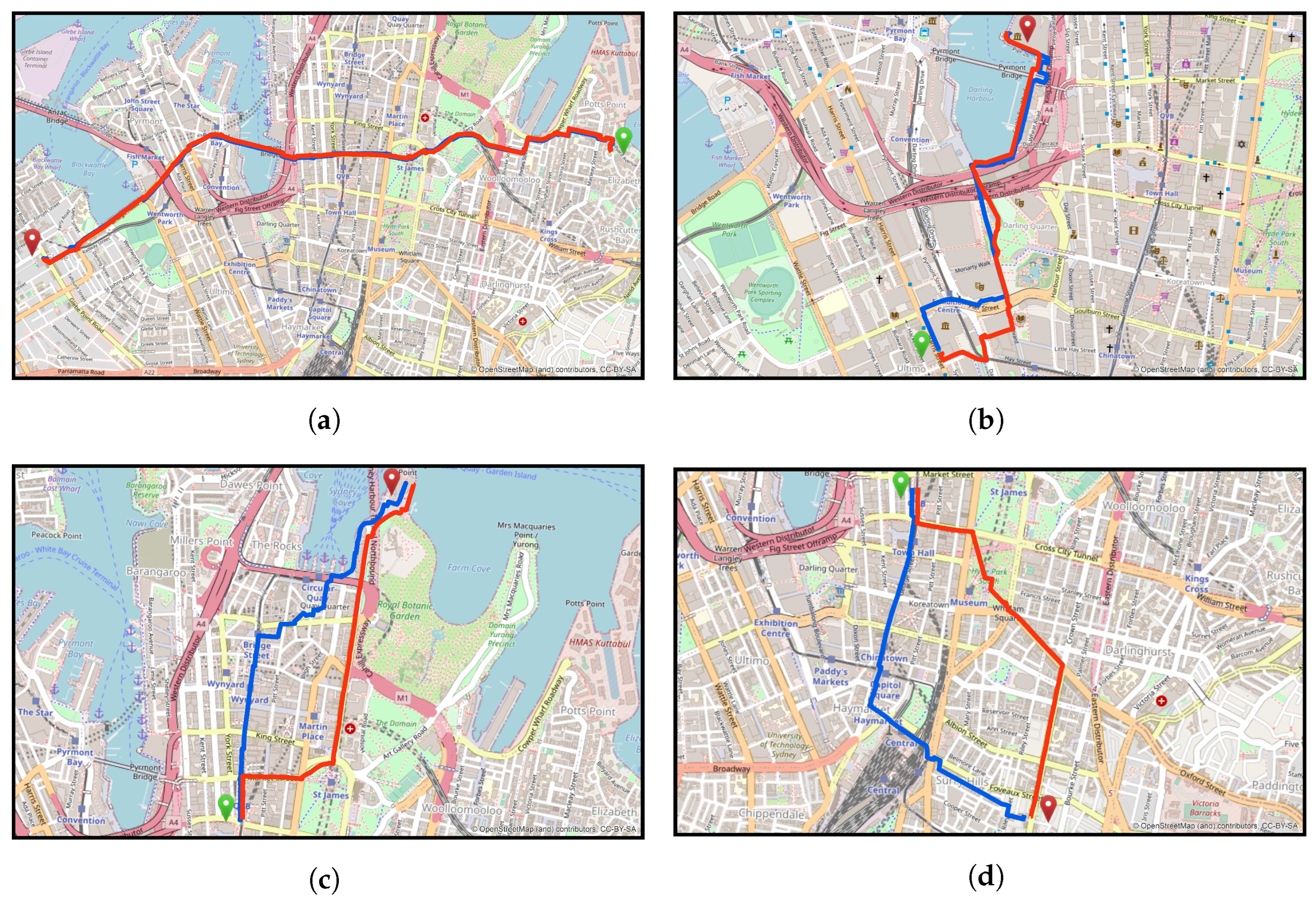
Figure 8 presents four route pairs grouped under different similarity clusters, and
Table 8 provides information on their main characteristics. According to
Figure 8a, the OSM route for “Elizabeth Bay House” to “Glebe Library” fully overlapped the Google Maps route by achieving a 40 m Hausdorff distance and a dissimilarity ratio of 0.87%. Despite deviations up to 157 m, the OSM route for “Powerhouse Museum” to “WILD LIFE Sydney Zoo” reached a 10.47% dissimilarity ratio as it was almost identical for most of the path (
Figure 8b). On the contrary, two OSM routes originating from the “Queen Victoria Building” to destinations “Sydney Opera House” (
Figure 8c) and “Surry Hills Library” (
Figure 8d) were dissimilar to Google Maps, accounting for 20.87% and 37.56%.
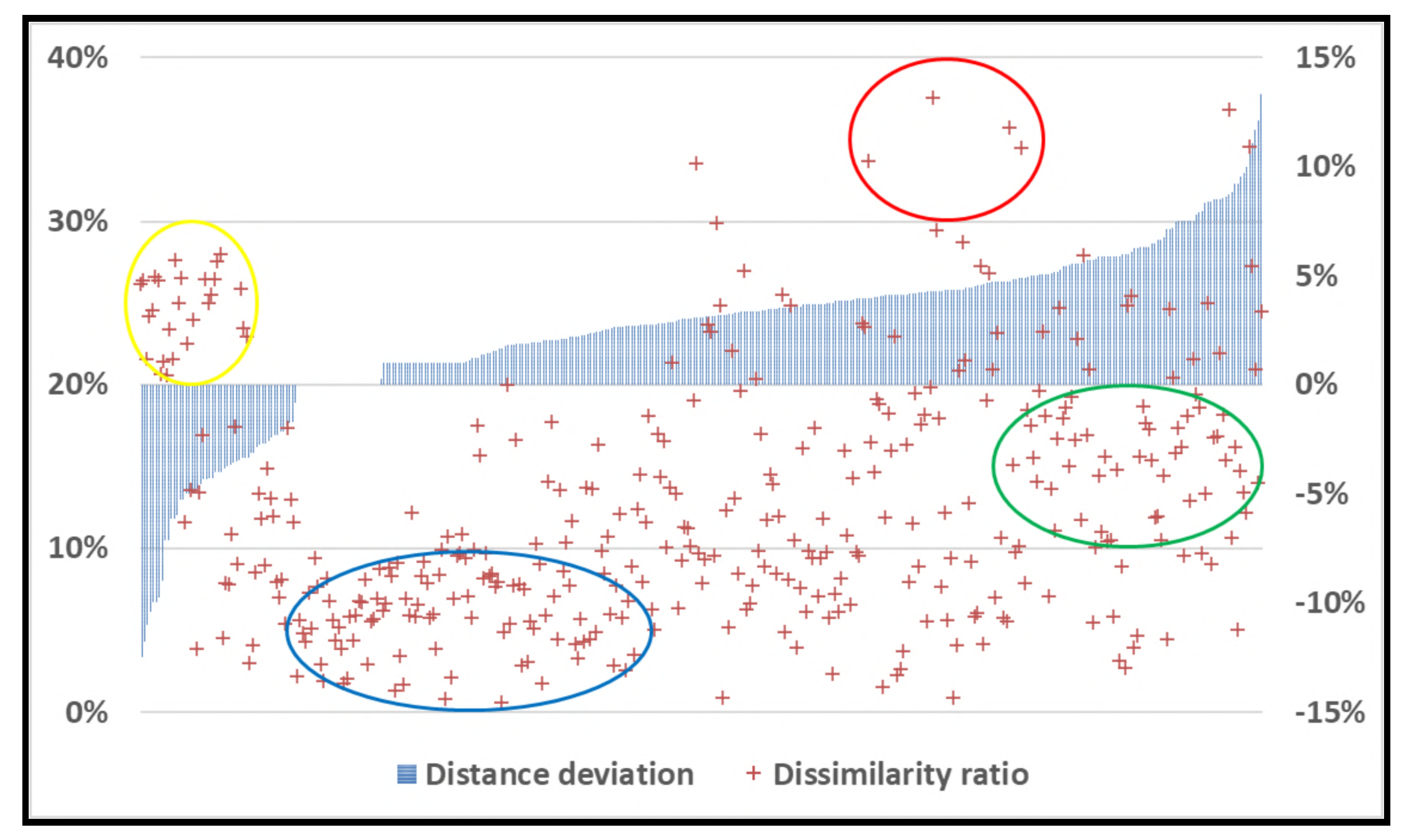
Figure 9 illustrates the relationship between the similarity of route pairs and their length deviation. The OSM shortest paths classified as well matched mainly concentrated between 0 and up to nearly 3% divergence from Google Maps (blue oval). A higher frequency of moderately matched occurrences was observed for OSM longer distances than Google Maps, with a maximum of 14.5% (green oval). The OSM routes shorter than Google Maps were mainly classified under the slightly matched cluster (yellow oval). Lastly, the red oval shows that all the non-matched routes occurred in the positive area of the plot.
According to
Table 9, on average, Google Maps witnessed straighter route geometry than OSM, achieving an average sinuosity index of nearly 1.41% versus 1.58%. The routes with a sinuosity index of over 1.8 could be challenging to walk. The Spearman’s rank correlation indicates a significant association between the sinuosity index and route length,
(758) = 0.92,
p < 0.001. Therefore, with an increase/decrease in route curviness, there is expected to be an increase/decrease in route length. Similarly, fewer road turns existed on Google Maps routes than OSM ones and, consequently, longer straight lines between each turn. On the other hand, OSM showed fewer intersections and lower average and maximum slopes than Google Maps.
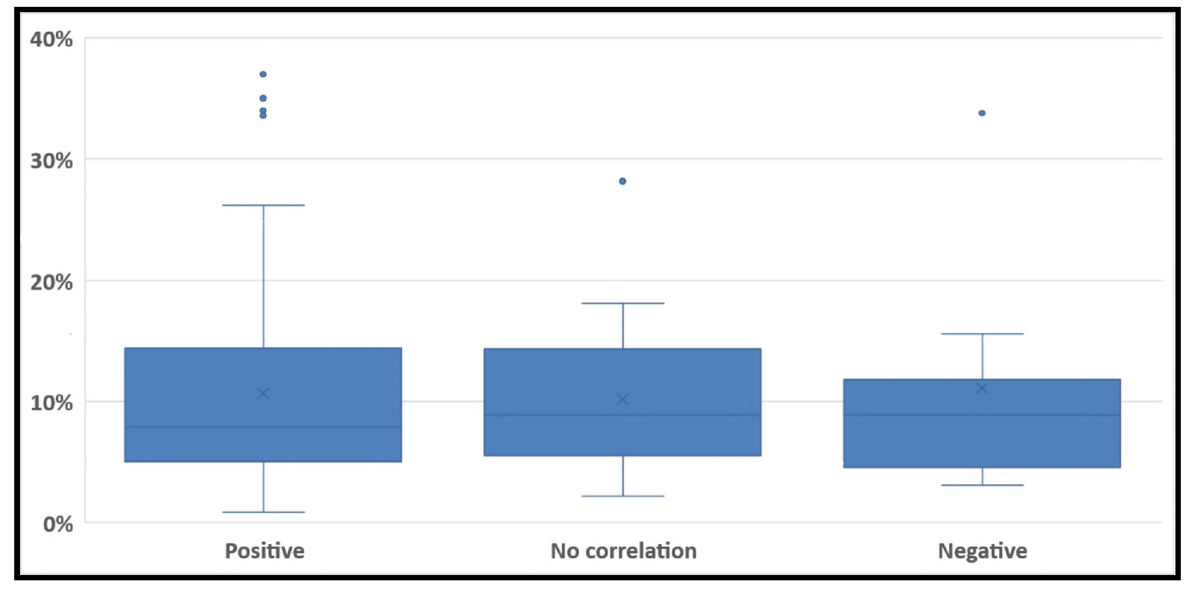
Figure 10 shows how the correlated findings between the sinuosity index and route length are distributed within different similarity clusters. According to
Table 10, one-way analysis of variance (ANOVA) indicates that the means of the three correlation groups were equal, F(2, 377) = 0.13,
p = 0.93.
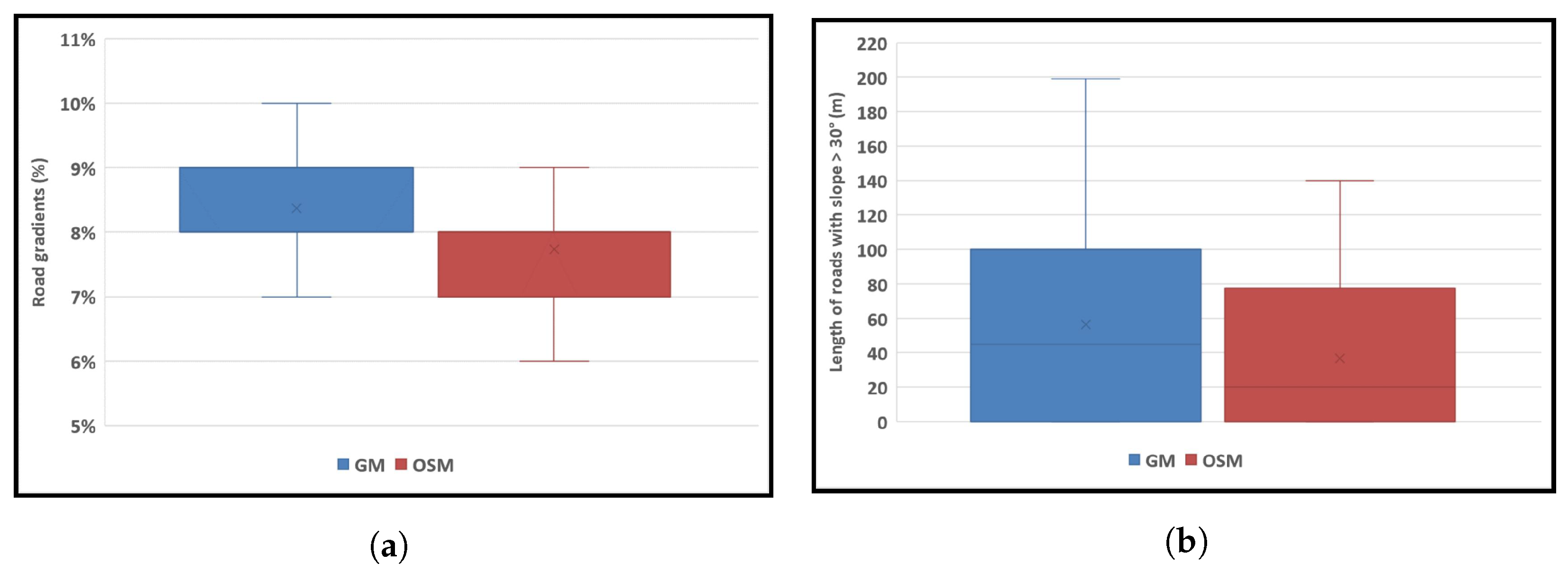
According to
Figure 11a, while the average road gradients were mainly between 7 and 9%, Google Maps experienced longer roads up to nearly 200 m with very steep slopes, which is more challenging to move than OSM for wheelchair users and older adults (
Figure 11b).
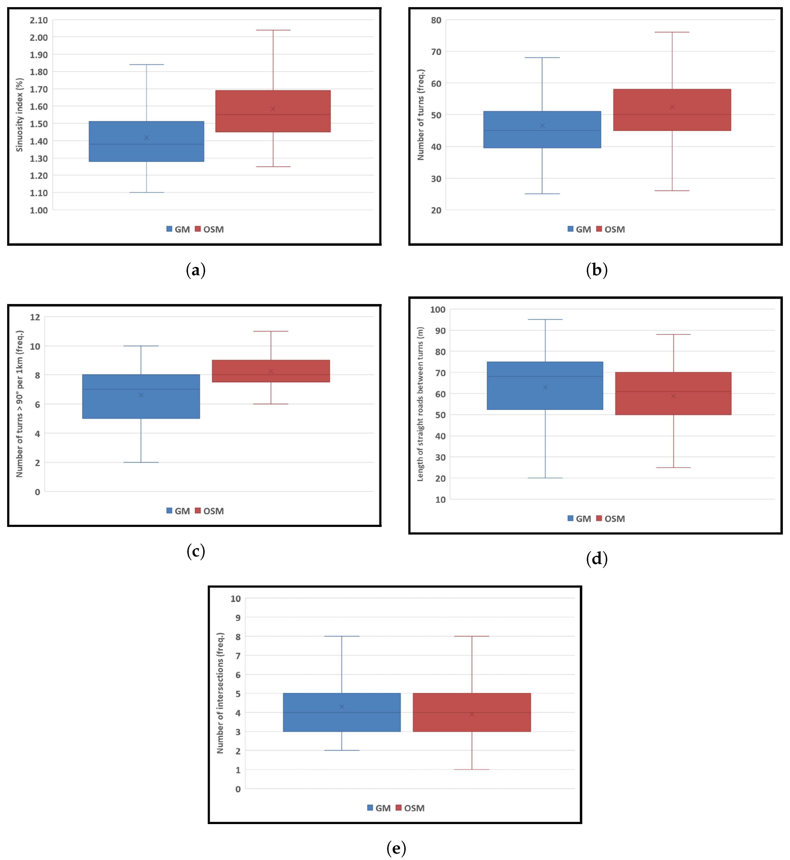
Moreover, Google Maps witnessed lower sinuosity indices compared to OSM, and half of the estimates were distributed between nearly 1.3–1.5% and 1.4–1.7%, respectively (
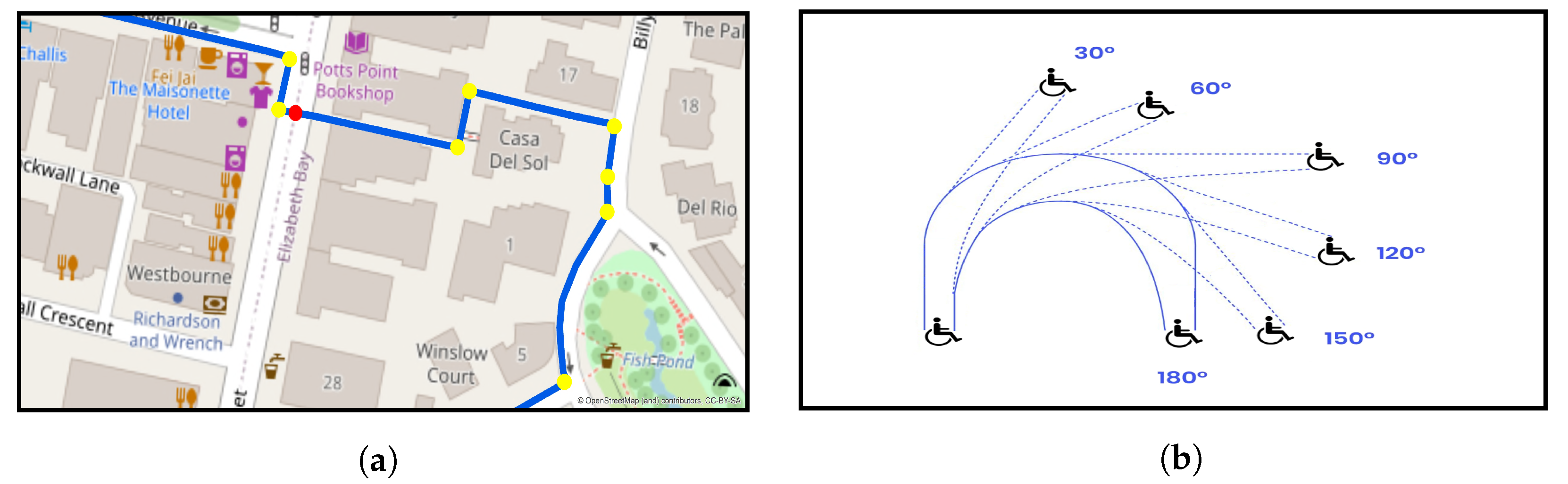
Figure 12a). There were not only more road turns with different degrees (i.e., 30
, 60
, 90
, 120
, 150
, and 180
) that existed on OSM than on Google Maps (
Figure 12b), but each route also had, at least, six 90
turns per kilometer (
Figure 12c), posing increased inconvenience and difficulty for wheelchair users. Meanwhile, three-fourths of OSM and Google Maps showed straight roads over 50 m up to about 90 m and 95 m between each directional change along the routes (
Figure 12d).
Figure 12e shows that both mapping services almost followed the same pattern regarding intersection frequency. However, there were some OSM routes with only one intersection.
4. Discussion
The shortest path analysis showed a closeness between the distance estimates of OSM and Google Maps, which could partly reflect the good quality of the OSM project’s data within the study area for pedestrian navigation services, especially those dependent on distance estimation. The observed differences can be justified based on the following reasons:
Road dataset’s characteristics
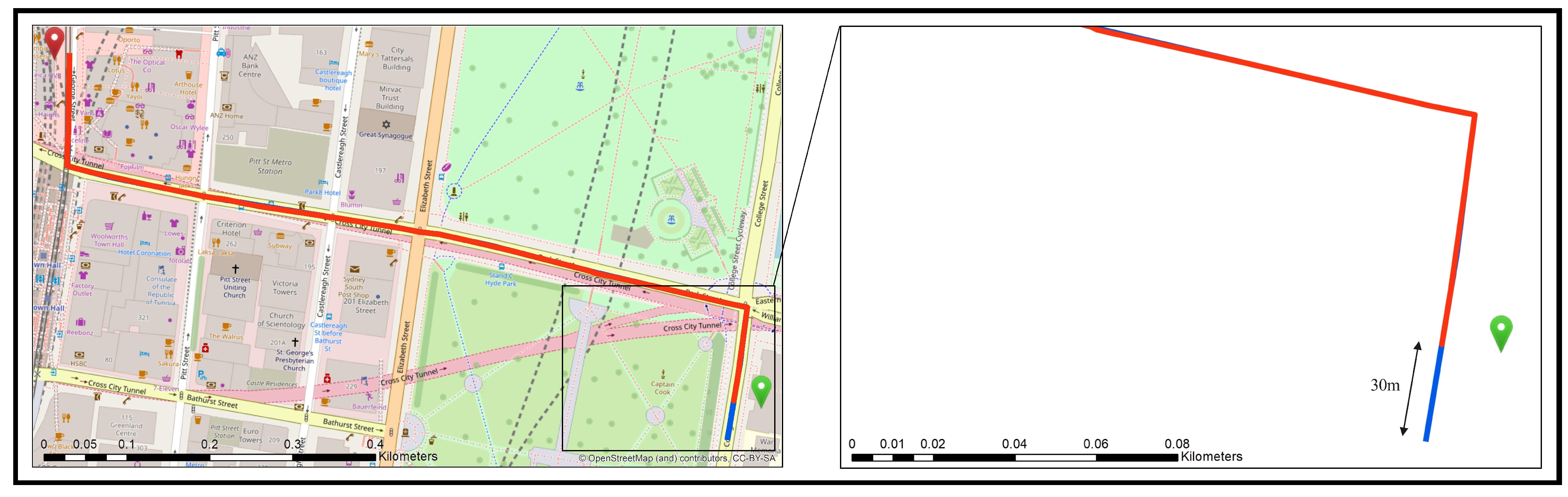
The data-related dissimilarities in route length might be derived from (a) differences in road density of networks or/and (b) existent topological inconsistencies in the dataset, such as unidentified connections and intersections. Moreover, (c) the starting/ending edges of calculated routes might have been placed in different positions (i.e., behind or ahead of the POI) for Google’s road dataset and OSM project’s data. As a result, it can be expected that the start or end of the route has yet to reach the exact position of the POI, or it conversely has gone beyond that (
Figure 13). Such a circumstance is more likely to occur to the POIs in areas inaccessible by the main street networks.
Utilized routing algorithm
Although both web mapping services use Dijkstra’s algorithm to calculate the shortest path between points A and B, the OSRM’s algorithm is a modified version of Dijkstra, namely, “MultiLevel Dijkstra (MLD)”, which works on the overlay graph (i.e., an approximation of the original graph with a reduced complexity) produced by a partitioning step. This could result in negligible differences in the lengths of the calculated routes.
Moreover, OSM was inclined to suggest the shortest paths remarkably similar to Google Maps in terms of geometry in such a way that about 90% of the calculated routes were identified as well matched and moderately matched. Nonetheless, the one-sample t-test indicates that the Hausdorff distances significantly differ from 0. It was not noticed any negative influence of the length parameter on the similarity of OSM routes to Google Maps ones. Conversely, almost all long routes with lengths up to 7.6 km appeared to be categorized under the well-matched class. A strong positive correlation was found between route curviness and route length, with an effect size of 0.92 percent. On average, OSM witnessed more tortuous routes and, thus, longer distances than Google Maps. Likewise, Google Maps offered longer straight roads between each turn than OSM, which is more suitable for pedestrians intending to evade frequent directional changes. On the contrary, OSM showed fewer intersections along the streets, thus, lowering the possibility of accidents. By choosing OSM over Google Maps, pedestrians are also expected to traverse the streets with lower road gradients and, thus, higher accessibility to the destination.
The metrics developed in this study, including the dissimilarity ratio and sinuosity index, demonstrated their practicability by quantifying the geometry properties of the shortest paths and offering helpful information for pedestrian navigation. Furthermore, providing further information on the number of road turns and intersections along the route and road gradients (extracted from open elevation data) could enable pedestrians to make wiser route choices according to their preferences, especially for mobility-impaired pedestrians, like wheelchair users and older adults.
5. Conclusions
Pedestrians might choose different routes for the same trip, depending on individual route choice preferences; while calculating the distance between locations A and B might be sufficient for most routing applications, route geometry information could also be important for specific types of pedestrians, especially those with limited mobility, like wheelchair users and older adults. Supplying realistic navigation services to these users requires that pedestrians be offered additional information on route geometry, helping them make more informed route choices. Focusing on open geospatial data, this study suggested an approach to extract and analyze the geometry information of the shortest pedestrian paths across four aspects: (a) similarity, (b) route curviness, (c) road turns and intersections, and (d) road gradients.
Stemming from the Hausdorff distance, the dissimilarity ratio quantified the geometry resemblance between pairs of the shortest pedestrian paths. A striking similarity was found between OSM and Google Maps, such that over half of the route pairs were almost identical. Moreover, a segment-based method measured the route curviness based on the number and degree of the road turns along the route. Spearman’s rank correlation indicated a direct association between route curviness and route length. Furthermore, the extracted road gradients from open elevation data showed the routes with more smoothness and better accessibility, while Google Maps showed less tortuosity and longer straight roads between bends, OSM could offer better choices when the frequency of road intersections and degree of road slopes are essential to pedestrians. The proposed geometry measures, including the dissimilarity ratio and sinuosity index, demonstrated their effectiveness by converting raw values into meaningful indicators. Personalized navigation systems are a target area of interest that can considerably benefit from the devised geometry metrics in this study.
The inadequacy and incompleteness of the OSM project regarding sidewalk information, such as surface type, width, and texture, among others, can be considered a limitation of this study. Such information could dramatically affect pedestrian route choices, given that good or poor sidewalk conditions might make movement easier or more challenging for pedestrians, especially wheelchair users; while little effort has been made to enrich sidewalk information in some countries [
25,
26,
27,
28], such data still need to be included in the OSM project for most parts of the world, including our case study, by launching data enrichment campaigns and projects.
Future studies could focus on (1) developing new methods and tools for extracting other information relevant to route geometry, (2) using them in current navigation systems, and (3) investigating how pedestrians benefit from them. Another area of work that could be much improved is (4) constructing a specialized road dataset for pedestrian navigation applications based on a combination of open geospatial sources, including OpenStreetMap, SpaceNet imagery, Google Earth Engine (GEE), and so on. Developing such a dataset could enable navigation systems to estimate more realistic pedestrian routes. Using computer vision models based on available satellite imagery data, like the SpaceNet dataset, could provide updates on road networks and sidewalk attributes far faster than terrestrial methods, especially in natural disasters or other dynamic events. Furthermore, extracting road elevation profiles from the GEE could be beneficial because providing such information allows pedestrians to make more informed route choices.

 ,
, 


