Article

PMGCN: Progressive Multi-Graph Convolutional Network for Traffic Forecasting

1
Faculty of Information Science and Engineering, Ocean University of China, Qingdao 266100, China
2
Laboratory for Regional Oceanography and Numerical Modeling, Qingdao National Laboratory for Marine Science and Technology, Qingdao 266237, China
3
Qingdao Real Estate Registration Center, Qingdao 266002, China
*
Author to whom correspondence should be addressed.
ISPRS Int. J. Geo-Inf. 2023, 12(6), 241; https://doi.org/10.3390/ijgi12060241
Submission received: 20 April 2023 / Revised: 9 June 2023 / Accepted: 15 June 2023 / Published: 16 June 2023

Abstract

:
Traffic forecasting has always been an important part of intelligent transportation systems. At present, spatiotemporal graph neural networks are widely used to capture spatiotemporal dependencies. However, most spatiotemporal graph neural networks use a single predefined matrix or a single self-generated matrix. It is difficult to obtain deeper spatial information by only relying on a single adjacency matrix. In this paper, we present a progressive multi-graph convolutional network (PMGCN), which includes spatiotemporal attention, multi-graph convolution, and multi-scale convolution modules. Specifically, we use a new spatiotemporal attention multi-graph convolution that can extract extensive and comprehensive dynamic spatial dependence between nodes, in which multiple graph convolutions adopt progressive connections and spatiotemporal attention dynamically adjusts each item of the Chebyshev polynomial in graph convolutions. In addition, multi-scale time convolution was added to obtain an extensive and comprehensive dynamic time dependence from multiple receptive field features. We used real datasets to predict traffic speed and traffic flow, and the results were compared with a variety of typical prediction models. PMGCN has the smallest Mean Absolute Error (MAE), Root Mean Squared Error (RMSE), and Mean Absolute Percentage Error (MAPE) results under different horizons (H = 15 min, 30 min, 60 min), which shows the superiority of the proposed model.

1. Introduction

Traffic forecasting has become an important task in intelligent transportation systems in recent years [1]. Accurate traffic forecasting is of great significance for the management and decision-making of intelligent transportation systems. In addition, the results of traffic prediction can also be used in many aspects of the city, such as spatial location optimization [2], measurement of traffic congestion [3], and so on. The most commonly used modes of traffic forecasting include traffic flow forecasting and traffic speed forecasting. Indeed, the complex and dynamic spatiotemporal dependencies of traffic data pose a challenge for the accuracy of traffic forecasts, owing to their inherent non-Euclidean structure. On the one hand, the spatial relationship between different regions is complex and may not only depend on the distance between nodes; on the other hand, the time-dependent relationship in the time dimension may not only be associated with fixed periodicity. Therefore, mining deep spatiotemporal relationship characteristics can improve complete traffic forecasting.
Methods for solving traffic forecasting tasks include an initial statistical method and traditional machine learning methods, such as ARIMA [4], SVR [5] and KNN [6,7]. Because these methods only consider time dependence and ignore other relations such as spatial dependence, their prediction accuracy is not high. At present, deep learning is primarily used, which can better deal with complex nonlinear relationships and extract spatial dependence. One such method is a grid-based method that first divides the study area into regular grids, uses a convolutional neural network (CNN) to extract spatial features, and uses a recurrent neural network (RNN) [8,9] to extract temporal features. Although CNN methods can capture a part of the spatial dependencies to some extent, it is challenging to extract spatial relations for a non-regular grid structure, such as traffic road networks.
Another method is to use a graph convolutional network (GCN) [10,11,12] to extract the spatial features. It is very helpful for dealing with non-Euclidean structures and is suitable for spatiotemporal correlation extraction of time series data of road networks. A spatiotemporal graph convolutional network is usually designed to apply a GCN to spatial relationship learning, and an RNN or one-dimensional CNN for time-dependent extraction [13,14,15]. However, most current GCN methods use a single adjacency matrix to reflect the complex spatial relationships between road networks, and such a method cannot obtain a comprehensive dynamic spatial relationship. For example, when affected by traffic events, the relationship between the same areas may change regularly over time, and only the spatial correlation in the local vicinity is considered; therefore, the extracted spatial relationship is not comprehensive. On this basis, some models add semantic information of external factors such as weather and POI [16], but the external semantic information is complex and rich and includes other factors (such as traffic congestion degree, road type, road intersection, geographical topography, etc.), and the semantic information about these external factors is also difficult to obtain. It is therefore not possible to take into account all the external semantic information at present. Some models also build a multi-graph architecture [17] to capture more comprehensive spatial dependencies, but the graph structure used either remains unchanged in different periods or can only reflect one internal aspect of the spatial structure relationship between nodes of the traffic network. Therefore, it remains impossible to effectively extract a comprehensive spatial correlation between nodes.
To overcome these shortcomings and achieve the extraction of dynamic and comprehensive spatiotemporal dependencies, we propose PMGCN, a progressive multigraph convolutional network model. Specifically, the model builds a multigraph convolutional network model based on multi-matrix spatiotemporal attention to learn spatial correlations among traffic nodes, and uses the channel attention mechanism and multi-scale 1DCNN to extract temporal correlations. In addition, a progressive connection relationship is designed between multigraph convolutions, which can efficiently extract spatial dependencies at a deep level, and at the same time, each spatial–temporal module is connected by a residual connection. In the multi-matrix structure, we use improved multi-head attention to dynamically adjust the predefined distance matrix, similarity matrix, and adaptive generation matrix, which can represent the relationship between spatial nodes more comprehensively. At the same time, the use of spatiotemporal attention to capture the spatiotemporal dependence can use the attention mechanism to highlight important spatiotemporal features, and produce more accurate traffic forecasting. The main contributions of this study are summarized as follows:
  • We designed a model of a progressive multi-graph convolutional network containing a multi-matrix spatiotemporal attention module, a multi-graph convolutional module, and a multi-scale temporal convolutional module. This model can extract a more comprehensive spatiotemporal dependency and capture dynamic changes between nodes more accurately.
  • We used a multi-matrix influence spatiotemporal attention by adaptively adjusting the spatial weights of the input of each order of the Chebyshev polynomial, which was used to dynamically extract the potential spatial correlation between traffic nodes. The distance matrix, similarity matrix, and adaptive matrix adjust the spatial weights from different angles. Among them, the adaptive matrix can be used to capture more comprehensive implied relationships. The spatiotemporal attention influenced by multiple matrices can enrich the ability of modeling spatiotemporal relationships, better capture spatiotemporal dependencies, and improve the prediction ability and prediction accuracy of the model.
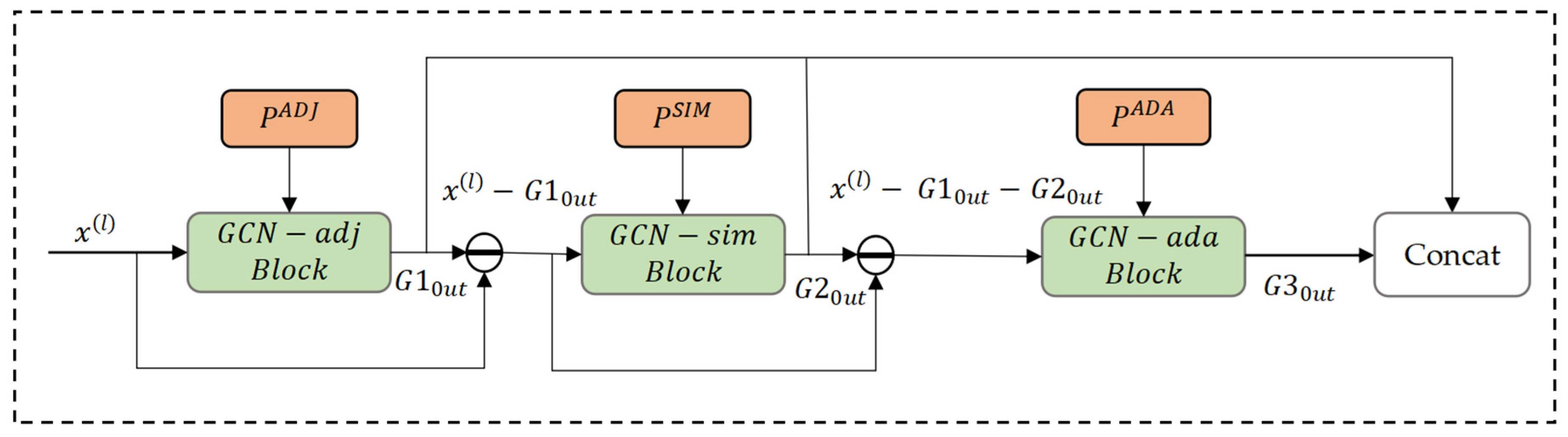
  • We propose a progressive connection between GCN blocks, where each GCN block removes the hidden information mined by the current GCN block, and the next GCN block mines the hidden information not mined by the previous GCN block. The sequence of multi-graph structure mining of hidden information is a distance graph, similarity graph, adaptive graph, and step-by-step deep extraction of spatial correlation between nodes. Among them, the adjacency graph focuses on the spatial correlation between adjacent local regions, the similarity graph expands from the physical distance between points from a global perspective, and the adaptive graph in the multi-graph model can further extract some complex and irregular spatial relationships affected by various factors.
  • To validate the effectiveness of the proposed model, extensive experiments were conducted using three real traffic datasets with two different traffic variables. The results show that the proposed method outperforms the existing methods.
The rest of the paper is organized as follows: Section 2 reviews related research on graph convolution, attention mechanisms, and traffic forecasting. Section 3 defines the problems addressed in this study. Section 4 introduces the proposed model in detail. Section 5 analyzes the experimental results and discusses the implications of the model’s main components. Section 6 provides a comprehensive summary of the study and future work.

2. Related Work

2.1. Graph Convolutional Neural Networks

At present, with the continuing maturity of deep learning, many researchers have transferred the traditional neural network model of Euclidean spatial data to the modeling of graph data, and automatically learned and extracted the features of graph data in an end-to-end manner, which plays a crucial role in dealing with the relationship between graph nodes and obtaining spatial topology information. Among these models, the graph convolutional neural network (GCN) is the most active and basic type in current research. The graph convolutional network performs the role of aggregation. Specifically, it can aggregate the characteristics of each node with its neighbors. It can be generally divided into two categories. The first is the spectral-based graph convolutional neural network proposed by Bruna et al. [18], who based their convolutional operation on the Laplacian extension of the spectral domain to the graph. To simplify the computation, ChebNet [19] uses the Chebyshev polynomial to approximate graph convolution. In a GCN [20], graph convolution enables the embedding of node attributes. Another type of graph convolutional neural network is based on the neighborhood aggregation space, which started earlier than research based on the spectral domain. In 2009, Micheli et al. [21] aggregated information for graph convolution, and Atwood et al. [10] introduced the concept of the diffusion process; the graph convolution was similar to a diffusion process. Zhu et al. [22] incorporate external features such as weather conditions and points of interest (POI) distribution into the GCN to generate more accurate results. In addition, Zhang et al. [23] used a graph attention network (GAT) to infer spatiotemporal relationships. These graph convolutional neural network models play an important role in capturing structural dependencies.

2.2. Attention Mechanism

The attention mechanism has efficient and flexible dependencies; therefore, it is widely used in various application fields. The attention mechanism works because it can focus on the most important parts of all information, rather than paying the same amount of attention to all information. Yan et al. [24] used an attention mechanism to aggregate local and global information. Zhou et al. [25] established that a spatiotemporal attention mechanism can adaptively select the most relevant citywide passenger demand information. Zheng et al. [26] also used a graph multi-attention network (GMAN) to extract correlations that exist in space and time. Liu et al. [27] effectively learned the spatiotemporal representation of traffic flow through an attention mechanism. Based on the series of developments of attention mechanisms mentioned above, we adopt a modified multi-headed attention mechanism for the dynamic extraction of traffic network features in this study.

2.3. Traffic Forecasting

Traffic forecasting has been extensively studied over the past few decades. In general, the challenge in traffic forecasting is to better capture dynamic temporal correlations and complex spatial dependencies. Methods such as ARIMA [28] were primarily used in the early period of traffic prediction research. With the need to capture nonlinear characteristics further, machine learning methods such as SVR [29] have shown better prediction effects. At present, deep learning methods have been widely used in capturing spatiotemporal correlations, such as CNN [30], LSTM [31], GCN [22], and GAN [32], combined with transfer learning [33] and meta learning [34]. Deep learning methods have significantly improved prediction accuracy. In this field, graph convolutional networks can make better use of graphs for information propagation and aggregation when dealing with traffic networks with complex topology. Therefore, graph convolutional networks are widely used in traffic prediction. For example, Yu et al. [14] proposed a spatiotemporal graph convolutional network (STGCN) that describes the traffic flow prediction problem with a graph to reduce the prediction error. Guo et al. [35] proposed an ASTGCN model, in which an attention mechanism was added to further improve the performance. Wang et al. [36] proposed the STMAG model, which can capture dynamic spatial correlations and combine a dynamic GCN with a location attention mechanism. Song et al. [37] proposed the spatiotemporal synchronous convolutional network model (STSGCN), which ignores the heterogeneity of data, and can effectively capture hidden spatiotemporal relationships. Zhang et al. [38] constructed a dynamic graph convolution based on spatiotemporal data embedding and proposed a new dynamic graph construction method to capture the correlation between nodes. Most existing spatiotemporal graph neural networks first construct an adjacency matrix determined by predefined measurements, and then learn from a predefined static single matrix. However, predefined matrices may not be sufficient to accurately describe the spatial relationships. To capture spatiotemporal accuracy, it is proposed to construct the adjacency matrix using learnable parameters. The adjacency matrix can change constantly, but the information extracted by a single adaptively generated adjacency matrix is one-sided. Currently, there are still some challenges in the comprehensive and dynamic extraction of spatial correlations.

3. Preliminaries

3.1. Problem Formulation

Traffic prediction tasks can be expressed as a typical spatiotemporal sequence prediction problem that aims to predict future traffic data (traffic flow, traffic speed, etc.) from observed historical traffic data. Given a historically observed traffic signal for P time-steps traffic signals, denoted as X = x t 1 , x t 2 , , x t p R P   ×   N   ×   C , our goal is to predict the next H time step traffic signals X = x t 1 , x t 2 , , x t p R P   ×   N   ×   C Y = x t p + 1 , x t p + 2 , , x t p + h R H   ×   N   ×   C . In addition, we define the concepts involved in the traffic forecasting problem as follows:
Definition 1. 
The traffic network is regarded as a weighted undirected graph G = ( V , E , A ) , where V represents all the graph nodes, indicating N observed sensors in the traffic network; E represents all the edges, indicating the connectivity among the observed sensors; and A R N   ×   N (weighted adjacency matrix) is a mathematical representation of the traffic network graph, indicating the correlation degree among the observed sensors.

3.2. Adjacency Matrices Construction

The first step in building a usable adjacency matrix is to analyze and mine traffic data to obtain the correlation between traffic nodes from different perspectives. We established three adjacency matrices: the distance adjacency matrix A A D J , similarity adjacency matrix A S I M , and adaptive adjacency matrix A A D A . First, the most basic measure of the spatial relationship of road networks relies on the distance between road networks, then a distance adjacency matrix A A D J is constructed based on the distance between road networks. In addition, traffic data are time series data, and the similarity of node time series can be used to characterize the similarity between nodes. In general, nodes with high degrees of similarity may exhibit similar traffic trends. In this paper, the Fast-DTW [39] approach was used to gauge the similarity of the time series of different nodes, and construct the similarity adjacency matrix A S I M . In general, the similarity of traffic patterns is not characterized by a single measurement but is also influenced by irregular accidental events and a variety of humanities and environments. Therefore, an adaptive matrix without any prior knowledge can extract hidden relationships at a deeper level. The adaptive matrix A A D A was constructed. The three matrices adjust the improved spatial attention mechanism to obtain more accurate and comprehensive spatiotemporal attention.

3.2.1. Distance Adjacency Matrix

The main method used to construct the adjacency matrix is to calculate the distance of the pairwise road network between the nodes, as shown in Equation (1). A threshold Gaussian kernel was used to build the distance adjacency matrix, as in Equation (2).
A A D J = A 11 a d j A 1 N a d j A i j a d j A 1 N a d j A N N a d j
A i j A D J = exp D i , j 2 v 2 , exp ( D i , j 2 v 2 ) ϵ 0 , O t h e r w i s e
where D ( i , j ) denotes the distance between node i and node j . ϵ denotes the threshold of the sparsity of the command matrix A A D J and ν is the standard deviation of the distance. A i j denotes the relationship weight between node i and node j .

3.2.2. Similar Adjacency Matrix

The similarity measures of time series can be divided into three categories: Euclidean distance based on time steps, dynamic time warps based on trend appearance based on shape images, and Gaussian mixture model (GMM) [40] based on change images. Dynamic time warping (DTW) is a typical time series similarity measurement algorithm. The DTW algorithm provides elastic alignment of two time series to find the best alignment and calculate the distance, but its time and space complexity is O (n2). Therefore, this study uses the fast dynamic time warping (Fast-DTW) method to calculate the similarity of time series and calculate the distance between time points of two time series. It finds an accurate approximation of the optimal wrap path between the two sequences. We used Fast-DTW to measure the similarity of nodes i and j in two time series X i and X j in Equation (3).
A S I M = A 11 s i m A 1 N s i m A i j s i m A 1 N s i m A N N s i m
Given two time series X i = ( x 1 i , x 2 i , , x n i ) and X j = ( x 1 j , x 2 j , , x m j ) , the state transition is:
D i , j = min D i 1 , j 1 , D i 1 , j , D i , j 1 + d ( i , j )
where d ( i , j ) denotes the distance between X i and X j . After several iterations, d i , j 1 2 is the similarity between time series X i and X j .
DTW is a dynamic programming-based algorithm whose core is to solve the warping curve, that is, the matching of sequence points X i and X j . The warping path ϕ can be expressed as follows (5):
ϕ = w 1 , w 2 , , w λ , max n , m λ n + m
The w determines the match between X i and X j , where λ is the item number in w and follows the property that max n , m λ n + m . This path minimizes the total distance between X i and X j . Finally, the DTW distance formula between two sequences X i and X j mentioned in TFGAN [41] is calculated as follows (6):
D T W ( X i , X j ) = m i n w 1 λ λ = 1 λ w λ

3.2.3. Adaptive Adjacency Matrix
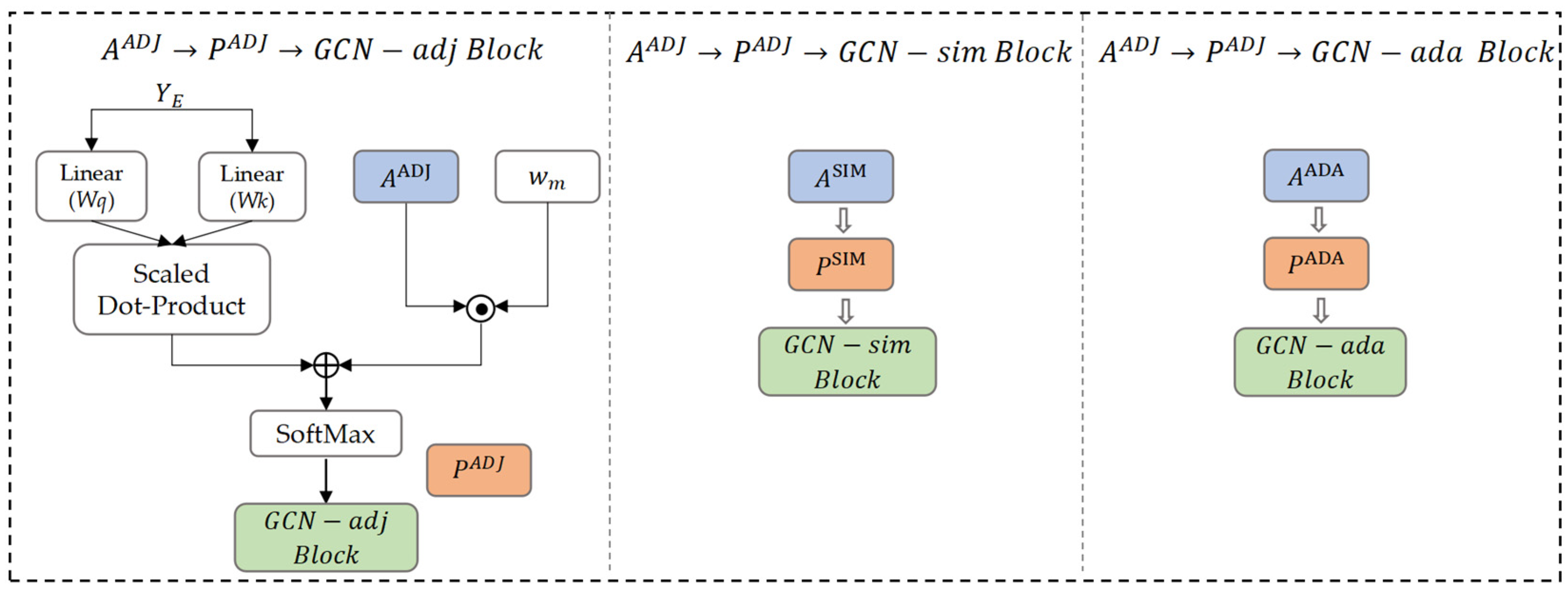
The adaptive adjacency matrix is an adjacency matrix without prior knowledge, which needs to be constructed using the node-embedding method, and is constructed according to Formula (7).
A a d a = S o f t M a x R e L U E 1 E 2 T
where E 1 , E 2 R N   ×   C represents the parameters generated by the random initialization. The S o f t M a x function is applied to normalize the adaptive adjacency matrices.

4. Methodology

This section first presents the framework of the proposed model and then introduces the details of each component in a stepwise manner.

4.1. Model Framework

Overall model framework: (1) The framework of the proposed model is illustrated in Figure 1. (2) The model consisted of multiple stacked spatiotemporal blocks. The spatiotemporal block mainly includes two parts: the spatiotemporal attention module and spatiotemporal convolution module. The residual connection is used between spatiotemporal blocks. Panel (a) shows the overall structure of PMGCN. Panels (b) and (c) show the details of the spatiotemporal block, where panel (b) describes the spatiotemporal attention (STA) module in the spatiotemporal block, which includes the temporal attention (TA) module and spatial attention (SA) module, and panel (c) outlines the spatiotemporal convolution (STC) module in the spatiotemporal block. The STC module includes two parts: a multi-graph convolutional layer and a multi-resolution channel attention temporal convolution. (3) The spatiotemporal correlation matrix A ( A A D J , A S I M , A A D A ) is constructed based on the distance proximity between traffic nodes and the similarity of the traffic node time series, as well as the continuous self-adaptation through training.
The spatiotemporal correlation matrix with correlation information between nodes was used in the SA, and the spatiotemporal attention was further adjusted. Three spatiotemporal correlation graphs were constructed using three spatiotemporal correlation matrices and applied to multi-graph convolution to obtain dependence information using dynamic space.

4.2. Spatiotemporal Block Model

Our PMGCN model is stacked with multiple spatiotemporal blocks, each of which includes spatiotemporal attention and spatiotemporal convolution modules, as shown in Figure 1. The spatiotemporal attention is used to capture the local dynamic changes between nodes and can provide the attention mechanism score for the multi-graph convolution layer in the spatiotemporal convolution module, making the spatial extraction more flexible and dynamic. In the spatiotemporal convolution module, multi-graph convolution extracts the spatial correlation, and multi-resolution one-dimensional convolution extracts the temporal dependence. Compared with a single graph and single resolution, the purpose of using multi-graph and multi-resolution is to extract a more comprehensive spatiotemporal dependence, and the operation efficiency of a one-dimensional convolution network is higher. Each part of the model structure is described in detail below.

4.2.1. Spatiotemporal Attention

As shown in Figure 1b, spatiotemporal attention comprises two parts: temporal and spatial attention. In this work, the road network is a network with multiple interconnected nodes, in which three types of adjacency matrices can provide accurate estimates of dependencies between nodes from different perspectives. However, the relationship between nodes is not static, and it is necessary to capture dynamic changes between nodes to obtain deep dynamic spatiotemporal dependencies. To this end, a spatiotemporal attention module that sequentially combines temporal and spatial attention was designed for our model.
Time attention: In the prediction of time series data, it is necessary to obtain not only the near correlation but also the remote correlation as much as possible. Multi-head self-attention allows the modeling of the correlation of elements in a sequence regardless of their distance and can have an effective global receptive field, providing a parallel mechanism. This mechanism can be used to effectively capture the complex dynamics of time series data, obtain long-range correlations, and achieve accurate long-term predictions. In addition, in considering the whole model, we also adopted the idea of residual attention [42] to enable the model to integrate shallow temporal dependence and deep temporal dependence. The temporal attention modules in adjacent ST blocks are connected to strengthen the temporal attention connection between the different ST blocks. This connection method can also alleviate the vanishing gradient problem, and can more effectively use the dynamic time dependence inside the traffic data. The multi-head attention definition and formula for the H-head are as follows (8): Q , K , V ϵ R c ( l 1 )   ×   T   ×   d are projected H times with H different matrices and stitched together to obtain O ϵ R c ( l 1 )   ×   T   ×   N   ×   d h . O concatenates the multi-head outputs of temporal attention and inputs them to the fully connected layer to obtain temporal attention O ϵ R c ( l 1 )   ×   T   ×   N . Finally, the residue between O and the input X ϵ R c ( l 1 )   ×   T   ×   N is performed, and the final output Y ϵ R c ( l 1 )   ×   T   ×   N is inputted into the spatial attention module through a normalization layer. The formulae are as follows (9)–(11):
A t t e n t i o n Q ( l ) , K ( l ) , V ( l ) = S o f t M a x A l V l ,       A ( l ) = Q ( l ) k ( l ) T d h + A ( l 1 )
O h = A t t e n t i o n Q W q ( h ) , K W q ( h ) , V W q ( h )
O = O ( 1 ) , O ( 2 ) , , O ( H )
Y 1 = L a y e r N o r m L i n e a r ( R e s h a p e ( O ) + X )
where Q ( l ) , K ( l ) , V ( l ) , and d h represent the query, keys, values, and dimensions, respectively. W q ( h ) ϵ R d   ×   d h , then O , represents the result of concatenating the multi-head outputs of temporal attention. O is the output of the temporal attention of O passing through the fully connected layer, and Y 1 is the final value passed into the spatial attention.
Spatial attention: The construction of the temporal attention module enabled us to obtain a feature representation with global dynamic time dependence. The spatial dependence is calculated from the output of the temporal attention module to obtain the feature expression of the dynamic spatial dependence Finally, the feature representation of the spatiotemporal attention dependence is obtained. In this study, we extend the self-attentive mechanism mentioned in the DSTAGNN [43], where multiple matrices are used to adjust the attention scores separately to obtain multiple spatial attentions. In simple terms, in contrast to the traditional self-attention mechanism, the weight coefficients calculated from the two branches of the input embedding vector (Q, K) were used to adjust the three adjacency matrices. The adjacency matrix with learning correlation adjusts the output attention of the final spatial module through parameter correction. As shown in Figure 1b, self-attention is not generated directly from the output Y 1 of the temporal attention module. Instead, Y 1 is first transposed, and then the time dimension M is mapped to a high-dimensional space d using one-dimensional convolution, and the feature dimension c l 1 is aggregated to obtain a two-dimensional matrix Y ϵ R N   ×   d E . Then, Y E is obtained through the embedding layer, and Y E is used to calculate the weight coefficient. The new spatial attention formula with H heads is given in Equations (12) and (13).
P h = S o f t M a x Y E W q ( h ) Y E W k ( h ) T d h + W m h A
p = p ( 1 ) , p ( 2 ) , , p ( H )
where W k ( h ) ϵ R d E   ×   d h and W q ( h ) ϵ R d E   ×   d h are learnable parameters, is the Hadamard product, W m h ϵ R N   ×   N is used to correct A to tune the attention of each head p ( h ) ϵ R N   ×   N , and the output p denotes the attention tensor, which is a combination of the outputs of each head. A is the general term of the represented matrix. There are three different matrices, and each matrix corresponds to a different attention score p obtained from A A D J P A D J , A S I M P S I M , A A D A P A D A . Details of the spatial attention module are shown in Figure 2.

4.2.2. Spatiotemporal Convolution

As shown in Figure 1c, the spatiotemporal convolution module in the PMGCN contains multi-graph convolution and multi-resolution one-dimensional convolution modules. During traffic forecasting, the state of a road network node at the next moment is influenced by the historical state of that node as well as the state of other nodes around it. Therefore, the relationship between nodes is both local and global, and capturing the potential spatiotemporal correlation and dependence under multiple relationships is a complex problem. To solve this problem, we adopted an interpretable multi-graph framework and a progressive connection method to capture spatial dependencies, a multi-scale 1DCNN, and a lightweight channel attention mechanism to comprehensively extract temporal dependencies.
Multi-graph convolution module: When using graph convolution to obtain the spatiotemporal correlation of traffic data, it is first necessary to construct a suitable graph. Different types of correlations between transportation network nodes can be obtained from different perspectives, and a graph can be constructed based on these correlations. Most of the existing studies still use a single matrix graph to represent the relationships that exist between nodes, which cannot capture the full range of spatiotemporal associations; therefore, we use a multi-graph architecture in our model. These are defined as follows:
Distance graph: In a real transportation network, the distance between stations can characterize the spatial relationship between nodes to a certain extent. In general, nodes that are closer together may have more influence on each other than nodes that are further apart. The traffic pattern changes may be similar between neighboring nodes (for example, the traffic nodes in the suburban areas on the edge of the city are less correlated with the traffic nodes in the congested areas in the center of the city, but the nodes close to each other in the suburban areas are more correlated). On this basis, the distance graph G C N A D J can be constructed, where the traffic road network nodes correspond to the points in the distance graph, and the edge between two nodes corresponds to the spatial distance between two road networks, and the formula is (2).
Similarity graph: In addition to using the basic distance relationship to characterize the relationship between nodes, the historical data relationship of the nodes can also be used. Under similar traffic conditions, there is a high probability of experiencing similar traffic patterns. Thus, by measuring the historical data of traffic nodes, the similarity graph G S I M is constructed by measuring the similarity between the sequences corresponding to each node. In the similarity graph, the edges between the nodes represent the similarity of traffic patterns between traffic nodes. The similarity matrix A S I M is given by Equation (3). Then, the DTW algorithm is used to calculate the correlation as shown in Equations (4)–(6). DTW calculates the shortest cumulative product distance between the historical data of each node. The correlation between sequences showed an opposite trend to the distance size. Using G S I M , the correlation between graph nodes can be modeled and extracted from the aspect of similarity.
Adaptive graph: When extracting the relationship between traffic nodes, the traffic mode of the nodes may be affected by various factors, such as geographical location, environment, and culture. Therefore, it is impossible to rely only on a single measurement angle; in this case, it is necessary to construct an adaptive graph G A D A to represent the complex relationship between nodes. This is different from other predefined graphs in that it constantly learns from training. The adaptive graph is used for the final convolution operation. Additional hidden spatial information can be mined using this information. Each traffic node in the graph represents a node in the adaptive graph, and the edge between two nodes represents the adaptive relationship. See calculation of Equation (7).
Graph convolutional network (GCN): Spatial graph convolution has a strong ability to aggregate adjacent node information to obtain node features. We used graph convolution based on the Chebyshev polynomial approximation to learn the node features of structure perception. As shown in Figure 1c, we adopted three GCN modules, which correspond to three different adjacency matrices: A A D J ,   A S I M ,   A A D A . Each GCN models the potential spatial correlation between nodes from a different perspective. Additionally, the attention P A D J , P S I M , and P A D A , corresponding to the G C N A D J , G C N S I M , and G C N A D A of each adjacency matrix in the space-time attention module, respectively, were used to dynamically adjust each term of the Chebyshev polynomial. In terms of spatial dimension, more meaningful and extensive features of the traffic network were extracted. In this study, the extended Laplacian matrix of the Chebyshev polynomial was defined as L = 2 , where A is the adjacency matrix, D is the degree matrix and I is the identity matrix.
L ~ = 2 λ m a x D A * I N
where A* is a general term for matrix, among which there are three matrices, A A D J ,   A S I M ,   A A D A . λ is the largest eigenvalue of L = ( D A * ) .
In a single graph convolution, information on each node is derived from nodes in its neighborhood. To incorporate the dynamic properties of the nodes, we aggregate the information from the graph signal x = x d by using the k t h order Chebyshev polynomial T , at each time step as follows:
g θ G x = g θ ( L ) x = k = 0 k 1 θ k T k ( L ~ ) p k x
g θ ϵ R k   ×   c ( l 1 )   ×   c l represents approximate convolution kernels, G is the convolution operation, which can learn vector θ ϵ R k which contains polynomial coefficients, and iteratively update in training. P is the spatiotemporal attention matrix of the k t h head. There are three different spatiotemporal attention matrices P corresponding to three different graph convolutional blocks P A D J G C N a d j ,   A S I M G C N s i m ,   A A D A G C N a d a . For the multi-channel input x ϵ R N   ×   c ( l 1 )   ×   T of this module, the features of each node have c ( l 1 ) channels, and g θ is the convolution kernel parameter [20]. Therefore, each node can aggregate information from neighboring nodes of order 0 ~ k 1 t h .
Progressive connections: The traffic network is complex and affected by many factors. Therefore, the integration of more information into a complex traffic network to extract spatiotemporal dependence is a key issue that needs to be addressed. A multigraph mechanism has emerged because a single graph cannot describe the association relationship well. At present, many multi-graph frameworks are used to fuse multiple graphs into a comprehensive graph for calculation [44,45] or to use a simple level number and parallel convolution. These methods simply fuse multiple graphs or stack multiple GCN blocks, which cannot mine the spatial dependence well and may cause the same spatial information to be continuously extracted. Therefore, a multi-graph framework with interpretable progressive connections was adopted in our model. The manner in which the multi-graphs were connected is shown in Figure 3. The input to the first GCN block is x l , the corresponding attention and the graph matrix, where the input of the next block is x l G 1 o u t . The input of the third graph is x l G 1 o u t G 2 o u t , and the GCN in each module takes a different graph matrix. The formula is as follows:
G x k + 1 = x l G 1 o u t G 2 o u t G k o u t
where G x k + 1 represents the input of the k t h graph convolution module.
In this study, three different graph structures are used, and they are connected in the order of distance, similarity, and adaptive graphs. Among them, the connection between the graph structure and graph structure uses a progressive connection method. The progressive connection can be interpreted as a way to extract only the s remaining information in the next graph structure that was not extracted in the previous graph structure; therefore, the output of each graph structure represents the information extracted in the current graph structure. The distance graph is used first because it contains the most basic information such as connectivity and distance between nodes; then, the similarity graph is used after the basic description of the transportation network, and the correlation between nodes is mined from the historical data of each node, from the perspective of the data sequence. Finally, deeper hidden spatial information was obtained. To adapt to the complex changes in the relationship between nodes at all times, an adaptive graph is used, which can continuously learn the graph from the training of the model, and is used to capture the remaining hidden relationships. Therefore, progressive connection is a method that can keep going deeper and deeper to obtain more hidden space, avoiding extracting the same spatial information between successive layers as much as possible.
Y 2 = R e l u ( L i n e a r ( G 1 o n t G 2 o n t G k o n t ) )
where G k o n t ϵ R N   ×   c ( l 1 )   ×   T represents the output of the k t h graph convolution module and Y 2 ϵ R N   ×   c ( l 1 )   ×   T represents the output of the whole multi-graph convolution module, which is then fed into the following multi-resolution temporal convolution module.
Multi-resolution convolution module: The time dependence between traffic nodes also needs to be focused on. Traffic conditions differ at different times. Therefore, in our model, after the multi-graph convolution module, we propose the addition of a multiscale convolutional network that combines channel attention. The multi-resolution convolution module combined with the channel attention mechanism mainly includes a multiscale temporal convolution and channel attention mechanism. The structure is shown in (c). One-dimensional CNNs with filters of different sizes and channel attentions are used in the multi-scale temporal convolution module to extract temporal dependencies. Multi-scale filters of different sizes allow the extraction of more comprehensive correlations. In addition, a channel focus mechanism is introduced to model the dependencies of the output channels and analyze the importance of the channels.
Multi-scale temporal convolution: The overall structure of the multi-resolution time block is shown in Figure 1c. Compared with RNN and other models, the one-dimensional CNN can greatly improve the training speed while effectively mining the temporal correlation. Our model also introduces an “Inception” structure with a multi-resolution convolutional neural network model, where the input data are filtered with three different sizes to obtain features at different scales. The input and the results of different convolutional calculations are concatenated together as the output, with three filters of 1 × 1, 1 × 3, and 1 × 5. The calculation formula is given as follows:
Z l = ϕ 1 Y 2 ( l 1 ) ϕ 2 Y 2 ( l 1 ) ϕ 3 Y 2 ( l 1 )
where Y 2 ( l 1 ) ϵ R c ( l 1 )   ×   N   ×   T is the input, ∗ is the convolutional operation, Z l ϵ R c ( l )   ×   N   ×   T is the output, and ϕ 1 ,   ϕ 2 ,   a n d   ϕ 3 are filters of different sizes.
To improve the performance of deep convolutional neural networks, a lightweight channel attention mechanism (ECA) [46] can obtain the correlation weights between channels. The ECA module is flexible to use, and in combination with inception, can further obtain the dependency values on multiple time scales and enhance the performance of the convolutional neural network, thus obtaining better performance in temporal dependency extraction. The calculation formula is provided as follows:
Z E = L i n e a r ( R e L U ( ω Z l ) ) = ω Z 1 , Z 2 , , Z C l
Z o u t ( l ) = L i n e a r ( R e L U ( Z E Y 2 ( l 1 ) ) )
where the output after the ECA module is Z E R C l   ×   N   ×   T , Z o u t ( l ) R C l   ×   N   ×   T is obtained after the activation function R e L U .

5. Experimental Studies

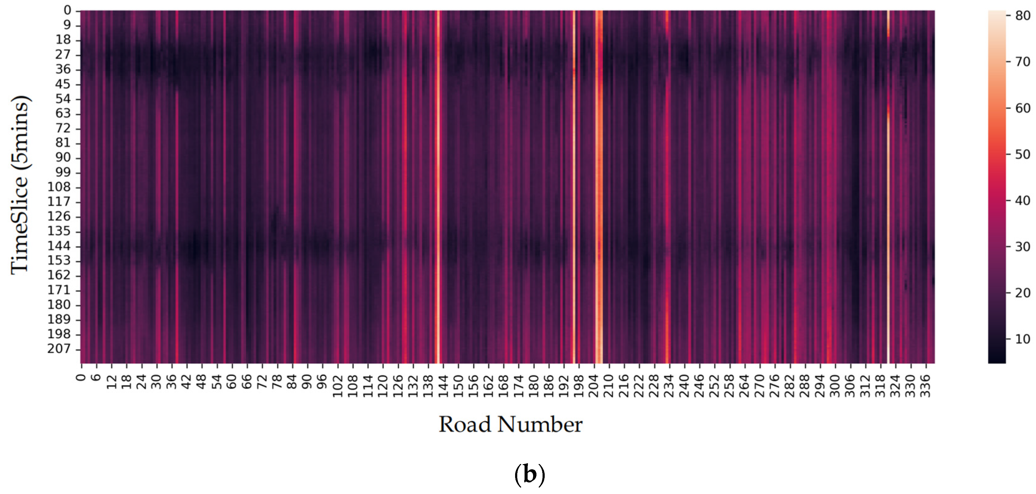
5.1. Experimental Data

In this section, the QingdaoGPS dataset is used to verify and analyze the performance of the model. The study area and the corresponding trunk roads are shown in Figure 4. In addition, PeMSD4 and PeMSD8 traffic flow datasets are used to further verify the effectiveness of the model.
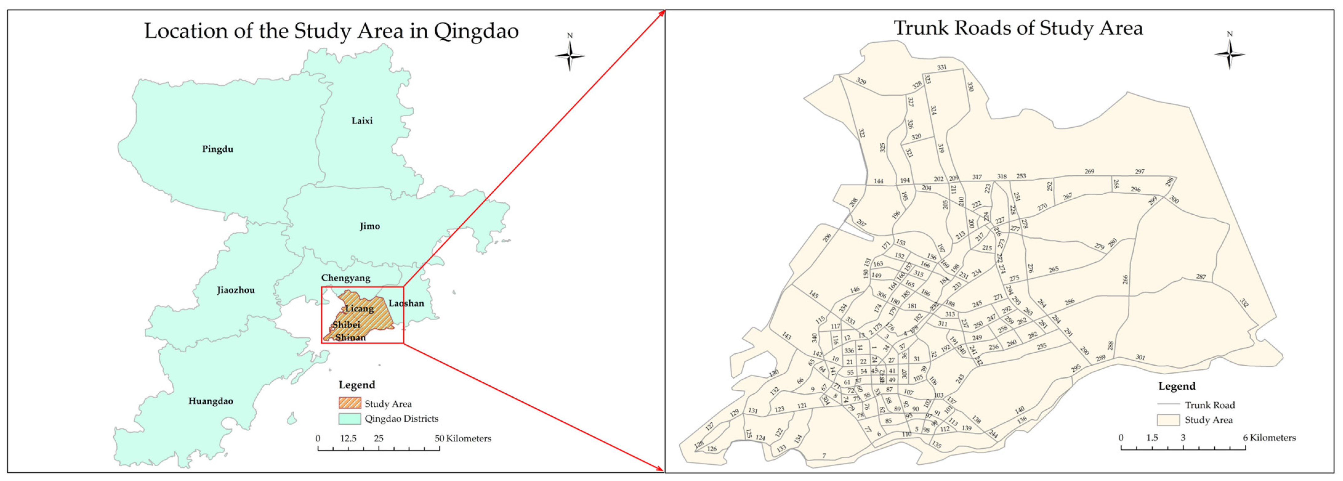
  • Trunk roads: We selected the main road network of Licang District, Shibei District, Shinan District, and the southwestern part of Laoshan District of Qingdao. The network consists of 340 trunk roads. We numbered each trunk road, from 1 to 340.
  • Traffic speed dataset: Real GPS data from Qingdao were used. These datasets were collected from the 340 main roads in Qingdao from 8 June 2020 to 26 July 2020. Table 1 presents the statistics in each row. The data contained taxi GPS records of the trunk roads. We reshaped the data into a time series by aggregating the average speed of the road network nodes every 5 min. In these datasets, each road network represents a node in the graph.
  • Traffic flow dataset: We used two real California traffic flow datasets. The PeMSD4 dataset includes 307 sensors, and the data were sampled from 1 January to 28 February 2018. The PeMSD8 dataset includes 170 sensors, and the data were sampled from 1 July to 31 August 2016. Detailed statistics are shown in Table 1.
The dataset was normalized using z-score normalization and split into training (60%), validation (20%), and test (20%) sets.

5.2. Experimental Setting

For the experiments in this study, we set the learning rate to 0.0001, the number of Chebyshev polynomials to 3, and the number of spatiotemporal attention heads to 3. The convolution kernel is along the temporal dimension (s = 1 × 1, s = 1 × 3, s = 1 × 5). All the graph convolution kernels used 32 convolution kernels. A stack of four ST modules was used for the experiments. The loss function used was the Huber loss, and the threshold parameter of the loss function was set to 1, while the batch size was set to 8. The hyperparameter of sparsity p = 0.01. We trained our model using the Adam optimizer. The prediction time was used to predict the traffic values for different future time periods (H = 3, 6, 12) using historical one-hour time steps (p = 12 steps). Three evaluation metrics were used to measure the performance of the model: mean absolute error (MAE), root mean squared error (RMSE), and mean absolute percentage error (MAPE). The evaluation criterion is that the lower the numerical result the better the model performance. The final experimental results were averaged over several repetitions. The calculation formula of the three evaluation indicators is as follows:
M A E = 1 n i = 1 n | Y i Y ^ i |
M A P E = 1 n i = 1 n Y i Y ^ i Y i
R M S E = 1 n i = 1 n ( | Y i Y ^ i ) 2
where Y i is true value; Y ^ i is predicted value; and n is number of data.

5.3. Baselines

We compared PMGCN with the following baselines, including both classical and advanced approaches in deep learning:
  • ARIMA: Autoregressive integrated moving average model [47];
  • FC-LSTM: The model uses a recurrent neural network with fully connected LSTM hidden units [48];
  • STGCN: Spatiotemporal graph convolutional network, using graph convolution and one-dimensional convolution [14];
  • ASTGCN: Introduces a spatiotemporal attention mechanism into the model, an attention-based spatiotemporal graph convolutional network model [35];
  • STSGCN: Spatiotemporal synchronous graph convolutional network, which utilizes local spatiotemporal subgraph modules to independently model local correlations, proposes a novel convolution operation to capture both spatial and temporal correlations [37];
  • ASTGNN: Attention-based spatiotemporal graph neural networks, we design a trend-aware self-attention to extract temporal dynamics and develop dynamic graph convolutions [49];
  • STGMN: Gated multi-graph attention spatiotemporal model, which uses multi-graph convolution and one-dimensional convolution for spatiotemporal extraction [50].
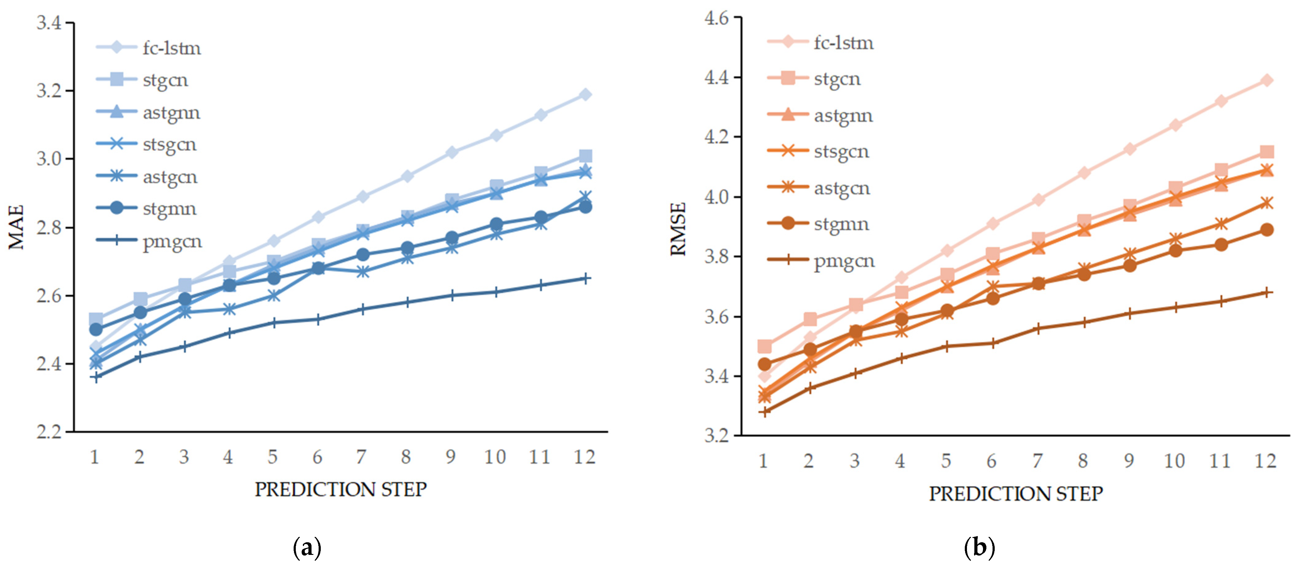
5.4. Main Results

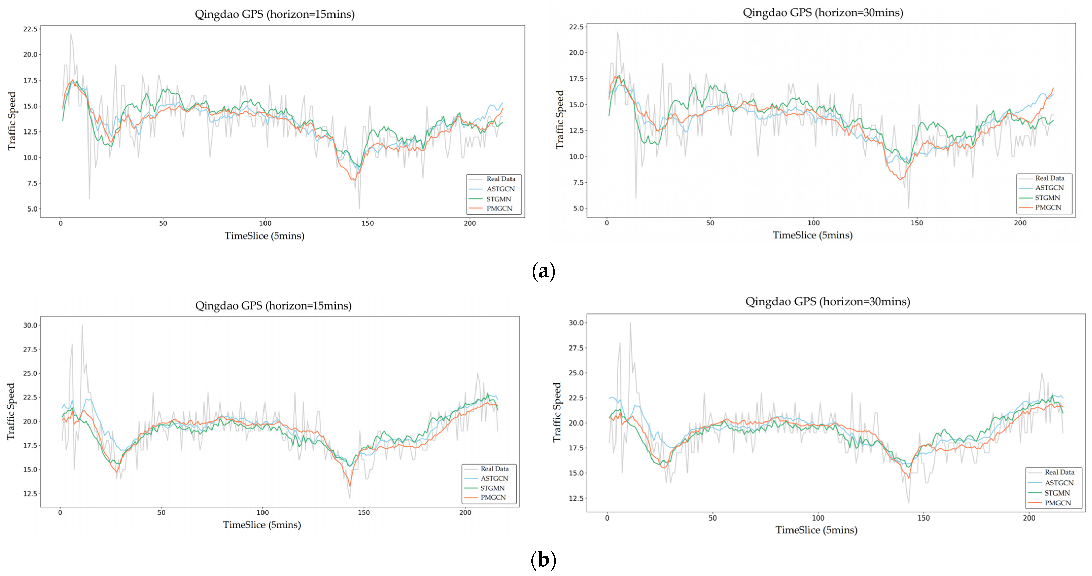
5.4.1. Different Models Prediction Performance

The main experimental results of the PMGCN and the compared baseline models on the traffic dataset are shown in Table 2. The experimental results at three different horizons (15 min, 30 min, and 60 min) were used to represent the prediction performance of the models for traffic speed modes. The experimental results in the table show that the prediction effect of the traditional model ARIMA is significantly lower than that of other deep learning models. First of all, in the deep learning baseline model, it is better to consider both time and space dependencies than to consider only time dependencies (e.g., FC-LSTM). Second, the results of using the graph convolution model to extract spatial dependencies are good, because graph convolution is well suited to extract hidden relationships between traffic nodes. In addition, using a spatiotemporal GCN model (e.g., STSGCN) is better for prediction than using a simple GCN. Moreover, with the addition of an attention mechanism (e.g., ASTGCN), good results are obtained in some aspects, and the use of a multi-graph framework in STGMN can obtain relatively good results at different horizons.
Compared with the baseline models, we propose that the PMGCN model adopt a new multi-graph architecture on the basis of the existing multi-graph architecture. It can learn the hidden deep dependency relationship between traffic nodes from multiple perspectives, such as spatial distance, node similarity and adaptive generation, and capture the dynamic changes between nodes by using spatiotemporal attention. Therefore, the final predictive performance PMGCN model is better than the baseline models. For instance, for the 60 min traffic speed forecasting task of the Qingdao GPS dataset in Table 2, the MAE values of ARIMA, FC-LSTM, STGCN, ASTGNN, STSGCN, ASTGCN, STGMN, and PMGCN were 3.31, 3.19, 3.01, 2.97, 2.96, 2.89, 2.86, and 2.65, respectively. PMGCN decreases the MAE in horizon 12 of Qingdao GPS by 20%, 17%, 12%, 11%, 10%, 8%, and 7% compared with the ARIMA, FC- LSTM, STGCN, ASTGNN, STSGCN, ASTGCN, and STGMN models, respectively.
To further demonstrate the effectiveness of the PMGCN, we plotted the prediction error results of all deep learning baseline models and PMGCN models at each step in the Qingdao GPS dataset as a line graph as shown in Figure 5. As shown in Figure 5, the PMGCN has the smallest prediction error at each step, while its curve is relatively smooth compared to the other models. The FC-LSTM model has the worst prediction effect among the baseline models. The prediction performances of the three baseline models STGCN, ASTGNN, and STSGCN are similar, and their prediction performance decreases significantly with a longer time step, which indicates the stability of the models in general. The model with the closest prediction effect to that of the PMGCN is STGMN, which also proves the effectiveness of the multi-graph convolution model. However, the prediction effect of STGMN was poor at the beginning, and its prediction effect in the first step was even lower than that of FC-LSTM.
To further demonstrate the effectiveness of the PMGCN, we also conducted prediction experiments using traffic flow datasets. The traffic flow prediction results of the PMGCN and the baseline models are presented in Table 3. On the two PEMS04 and PEMS08 datasets, our PMGCN achieved the best results for most indicators. The main reason for this comes from the aforementioned use of different GCN blocks to extract various complex correlations, and the addition of a multi-resolution temporal convolution module for temporal correlation extraction also greatly improves the operation efficiency compared to other time extraction models. Compared with the FC-LSTM, STGCN, ASTGCN, STSGCN, and STGMN models, PMGCN reduced the RMSE of PeMSD4 by 32%, 20%, 14%, 13%, and 9%, respectively, at horizon 12. The RMSE of PeMSD8 was also reduced by 33%, 28%, 17%, 10%, and 7% at horizon 12, respectively. The main reason for this is that the PMGCN establishes dependencies with neighboring and global nodes.

5.4.2. Analysis of Model Prediction Results
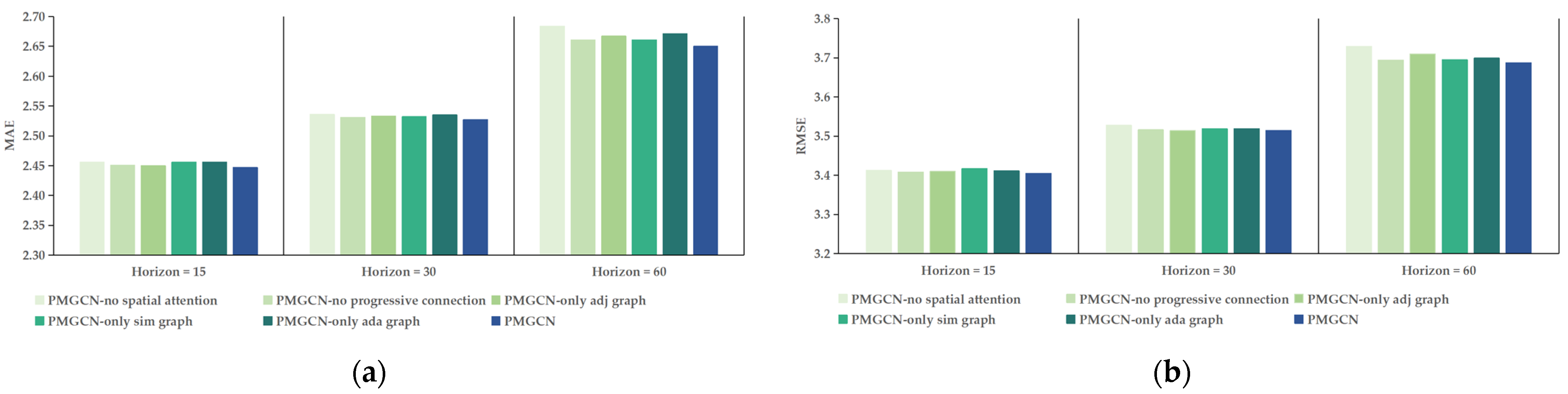
According to the prediction effects of different models, the effectiveness of PMGCN model can be seen. In this section, we explore the results predicted by the PMGCN model. Figure 6 and Figure 7 show the real and predicted visualization results for 340 trunk roads on non-working days and working days. We choose 6:00 a.m. to 12:00 p.m. as the study period, according to human activities during those times. The time interval in this study was 5 min, so there were 216 time slices in a day. By visualizing the results, we find that there is no obvious morning and evening peak during non-working days. However, there are obvious morning and evening peaks on weekdays, mainly concentrated in the 18–36 time slice and the 135–153 time slice, that is, the morning peak occurs from about 7:30 a.m. to 9:00 a.m., and the evening peak occurs from about 5:15 p.m. to 6:45 p.m. In addition, it can be seen from Figure 7 that the average speed of several trunk roads is significantly lower than those of other trunk roads, such as 42–48, 67–68, 71–74, 98–99, 108–110, 114–117, 222–228, 308–310. At the same time, there are several trunk roads with significantly higher average speed than other trunk roads, such as 142–143, 197, 206–208, 322. For this reason, we chose the trunk road numbered 71 and the trunk road numbered 110 for further visualization. According to the MAE and RMSE of different models, three relatively good models can be obtained, namely, ASTGCN, STGMN, and PMGCN. Figure 8 illustrates the prediction results of the three models at the same node. The prediction effect of the STGMN model is closest to that of the PMGCN model. It is better than PMGCN in some details, but PMGCN is more stable and better judging from the overall trend, especially when there are major changes (i.e., during spikes). Therefore, PMGCN can capture the dynamic changes of the speed pattern more accurately, and it can also have more of an advantage in special road sections.

5.5. Ablation Study

The PMGCN model comprises different components, each of which plays a role in extracting spatiotemporal dependencies. To verify the effectiveness of each component, we conducted ablation experiments on the Qingdao GPS dataset and compared the following PMGCN variants:
  • PMGCN-only adj graph: We used the distance graph only in space-time blocks;
  • PMGCN-only sim graph: We used the similarity graph only in spatiotemporal blocks;
  • PMGCN-only ada graph: We only used the adaptive graph in spatiotemporal blocks;
  • PMGCN-no progressive connection: Only pure stacking was used, without progressive connection;
  • PMGCN-no spatial attention: Lack of spatial attention layer dynamically adjusts each term in the graph convolution.
The MAE and RMSE prediction errors of PMGCN and its variants for the Qingdao GPS data are shown in Figure 9. It is obvious that the extraction of only one GCN module is not as good as the prediction using multiple GCN modules. It can be seen from Figure 9 that the MAE of the PMGCN-only adj graph, PMGCN-only sim graph, and PMGCN-only ada graph are roughly 2.667, 2.661, and 2.671, respectively, at horizon 12, while the PMGCN is 2.650 at the unified horizon. Similarly, removing the spatial attention and no longer dynamically adjusting each term in the graph convolution increases the RMSE from 3.687 to 3.729 for the PMGCN. In summary, the PMGCN outperformed other variables in terms of prediction accuracy, indicating that the PMGCN can capture hidden and complex correlations and produce accurate predictions.

6. Conclusions and Future Work

To improve the accuracy of traffic prediction, this study introduces an effective progressive spatiotemporal attention multi-graph convolutional network (PMGCN) model. In contrast to existing traffic prediction models, PMGCN establishes various adjacency matrices with multiple GCNs from different perspectives, such as the distance between traffic nodes, the similarity of time series data, and adaptive generation, which is used to extract the deep implicit correlation between traffic nodes. The attention score obtained by the spatiotemporal attention module dynamically adjusts each term of the Chebyshev polynomial in the graph convolution, which can capture the dynamics between traffic nodes more accurately. In addition, a multi-resolution one-dimensional convolutional network is used to extract the time-dependence between nodes, which is more efficient than other time-dependence extraction models. The experimental results on real datasets in this study show that PMGCN has a better performance than the relevant baseline model.
Our model has the following limitations: (1) More comprehensive external semantics were not added; (2) The verification experiment only covered two modes of traffic speed and traffic flow, which need to be further verified for applicability; (3) The impact on special time periods (such as morning and evening peak hours) was not considered in detail. Future work will include selecting relevant semantic information and integrating it into the model, studying the adaptability of other traffic modes and other cities, considering special time periods for modeling and prediction performance evaluation. We need to further explore and improve the deep learning model so that it can be applied to the wider field of traffic forecasting.

Author Contributions

Conceptualization, Zhenxin Li and Yong Han; Data curation, Zhenxin Li; Formal analysis, Zhenxin Li and Zhenyu Xu; Funding acquisition, Yong Han; Investigation, Zhenxin Li; Methodology, Zhenxin Li and Zhenyu Xu; Project administration, Yong Han; Resources, Yong Han; Software, Zhenxin Li; Supervision, Ge Chen; Validation, Zhenxin Li and Zhihao Zhang; Visualization, Zhenxin Li and Zhixian Sun; Writing—original draft, Zhenxin Li; Writing—review and editing, Zhenxin Li, Zhenyu Xu and Zhihao Zhang. All authors have read and agreed to the published version of the manuscript.

Funding

This research was funded by the Natural Science Foundation of Shandong Province, China (Grant No. ZR2020MD020).

Institutional Review Board Statement

Not applicable.

Informed Consent Statement

Not applicable.

Data Availability Statement

Not applicable.

Conflicts of Interest

The authors declare no conflict of interest.

References

  1. Gu, Y.; Deng, L. STAGCN: Spatial–Temporal Attention Graph Convolution Network for Traffic Forecasting. Mathematics 2022, 10, 1599. [Google Scholar] [CrossRef]
  2. Chen, Y.; Wu, G.; Chen, Y.; Xia, Z. Spatial location optimization of fire stations with traffic status and urban functional areas. Appl. Spat. Anal. Policy. 2023, 16, 771–788. [Google Scholar] [CrossRef]
  3. Wang, Y.; Tong, D.; Li, W.; Liu, Y. Optimizing the spatial relocation of hospitals to reduce urban traffic congestion: A case study of Beijing. Trans. GIS 2019, 23, 365–386. [Google Scholar] [CrossRef]
  4. Ding, Q.Y.; Wang, X.F.; Zhang, X.Y.; Sun, Z.Q. Forecasting Traffic Volume with Space-Time ARIMA Model. Adv. Mater. Res. 2011, 156–157, 979–983. [Google Scholar] [CrossRef]
  5. Wu, C.H.; Ho, J.M.; Lee, D.T. Travel-time prediction with support vector regression. IEEE Trans. Intell. Transp. Syst. 2004, 5, 276–281. [Google Scholar] [CrossRef] [Green Version]
  6. Cheng, S.; Lu, F.; Peng, P.; Wu, S. Short-term traffic forecasting: An adaptive ST-KNN model that considers spatial heterogeneity. Comput. Environ. Urban Syst. 2018, 71, 186–198. [Google Scholar] [CrossRef]
  7. Cheng, S.; Lu, F.; Peng, P.; Wu, S. A Spatiotemporal Multi-View-Based Learning Method for Short-Term Traffic Forecasting. ISPRS Int. J. Geo-Inf. 2018, 7, 218. [Google Scholar] [CrossRef] [Green Version]
  8. Zhang, J.; Zheng, Y.; Qi, D.; Li, R.; Yi, X. DNN-based prediction model for spatio-temporal data. In Proceedings of the 24th ACM SIGSPATIAL International Conference on Advances in Geographic Information Systems, Burlingame, CA, USA, 31 October–3 November 2016; p. 92. [Google Scholar]
  9. Li, Y.; Shahabi, C. A brief overview of machine learning methods for short-term traffic forecasting and future directions. Sigspatial Spec. 2018, 10, 3–9. [Google Scholar] [CrossRef]
  10. Li, Z.; Xiong, G.; Chen, Y.; Lv, Y.; Hu, B.; Zhu, F.; Wang, F.-Y. A Hybrid Deep Learning Approach with GCN and LSTM for Traffic Flow Prediction. In Proceedings of the 2019 IEEE Intelligent Transportation Systems Conference, ITSC 2019, Auckland, New Zealand, 27–30 October 2019; pp. 1929–1933. [Google Scholar]
  11. Huang, R.; Huang, C.; Liu, Y.; Dai, G.; Kong, W. LSGCN: Long Short-Term Traffic Prediction with Graph Convolutional Networks. In Proceedings of the 29th International Joint Conference on Artificial Intelligence, Yokohama, Japan, 7–15 January 2020; pp. 2355–2361. [Google Scholar]
  12. Wang, X.; Ma, Y.; Wang, Y.; Jin, W.; Wang, X.; Tang, J.; Jia, C.; Yu, J. Traffic Flow Prediction via Spatial Temporal Graph Neural Network. In Proceedings of the 29th World Wide Web Conference (WWW), Taipei, Taiwan, 20–24 April 2020; pp. 1082–1092. [Google Scholar]
  13. Atwood, J.; Towsley, D. Diffusion-Convolutional Neural Networks. In Proceedings of the 30th Conference on Neural Information Processing Systems (NIPS 2016), Barcelona, Spain, 5–10 December 2016. [Google Scholar]
  14. Yu, B.; Yin, H.; Zhu, Z. Spatio-temporal graph convolutional networks: A deep learning framework for traffic forecasting. arXiv 2017, arXiv:1709.04875. [Google Scholar]
  15. Zhao, L.; Song, Y.; Zhang, C.; Liu, Y.; Wang, P.; Lin, T.; Li, H. T-gcn: A temporal graph convolutional network for traffic prediction. IEEE Trans. Intell. Transp. Syst. 2019, 21, 3848–3858. [Google Scholar] [CrossRef] [Green Version]
  16. Zhu, J.; Han, X.; Deng, H.; Tao, C.; Zhao, L.; Wang, P.; Lin, T.; Li, H. KST-GCN: A knowledge-driven spatial-temporal graph convolutional network for traffic forecasting. IEEE Trans. Intell. Transp. Syst. 2022, 23, 15055–15065. [Google Scholar] [CrossRef]
  17. Lee, K.; Rhee, W. DDP-GCN: Multi-graph convolutional network for spatiotemporal traffic forecasting. Transp. Res. Part C Emerg. Technol. 2022, 134, 103466. [Google Scholar] [CrossRef]
  18. Bruna, J.; Zaremba, W.; Szlam, A.; LeCun, Y. Spectral networks and locally connected networks on graphs. arXiv 2013, arXiv:1312.6203. [Google Scholar]
  19. Defferrard, M.; Bresson, X.; Vandergheynst, P. Convolutional Neural Networks on Graphs with Fast Localized Spectral Filtering. Adv. Neural Inf. Process. Syst. 2016, 29, 3844–3852. [Google Scholar]
  20. Kipf, T.N.; Welling, M. Semi-Supervised Classification with Graph Convolutional Networks. In Proceedings of the International Conference on Learning Representations (ICLR), Toulon, France, 24–26 April 2017. [Google Scholar]
  21. Micheli, A. Neural Network for Graphs: A Contextual Constructive Approach. IEEE Trans. Neural Netw. 2009, 20, 498–511. [Google Scholar] [CrossRef]
  22. Zhu, J.; Wang, Q.; Tao, C.; Deng, H.; Zhao, L.; Li, H. AST-GCN: Attribute-augmented spatiotemporal graph convolutional network for traffic forecasting. IEEE Access 2021, 9, 35973–35983. [Google Scholar] [CrossRef]
  23. Zhang, K.; He, F.; Zhang, Z.; Lin, X.; Li, M. Graph Attention Temporal Convolutional Network for Traffic Speed Forecasting on Road Networks. Transp. B Transp. Dyn. 2021, 9, 153–171. [Google Scholar] [CrossRef]
  24. Yan, X.; Zheng, C.; Li, Z.; Wang, S.; Cui, S. Pointasnl: Robust point clouds processing using nonlocal neural networks with adaptive sampling. In Proceedings of the IEEE/CVF Conference on Computer Vision and Pattern Recognition, Seattle, WA, USA, 13–19 June 2020; pp. 5589–5598. [Google Scholar]
  25. Zhou, Y.; Li, J.; Chen, H.; Wu, Y.; Wu, J.; Chen, L. A spatiotemporal attention mechanism-based model for multi-step citywide passenger demand prediction. Inf. Sci. 2020, 513, 372–385. [Google Scholar] [CrossRef]
  26. Zheng, C.; Fan, X.; Wang, C.; Qi, J. Gman: A graph multi-attention network for traffic prediction. In Proceedings of the AAAI Conference on Artificial Intelligence, New York, NY, USA, 7–12 February 2020; Volume 34, pp. 1234–1241. [Google Scholar]
  27. Liu, L.; Zhen, J.; Li, G.; Zhan, G.; He, Z.; Du, B.; Lin, L. Dynamic spatial-temporal representation learning for traffic flow prediction. IEEE Trans. Intell. Transp. Syst. 2020, 22, 7169–7183. [Google Scholar] [CrossRef]
  28. Williams, B.M.; Hoel, L.A. Modeling and forecasting vehicular traffic flow as a seasonal ARIMA process: Theoretical basis and empirical results. J. Transp. Eng. 2003, 129, 664–672. [Google Scholar] [CrossRef] [Green Version]
  29. Ahn, J.Y.; Ko, E.; Kim, E. Predicting spatiotemporal traffic flow based on support vector regression and Bayesian classifier. In Proceedings of the IEEE 5th International Conference on Big Data and Cloud Computing, Dalian, China, 26–28 August 2015; pp. 125–130. [Google Scholar]
  30. Ma, X.; Dai, Z.; He, Z.; Ma, J.; Wang, Y.; Wang, Y. Learning Traffic as Images: A Deep Convolutional Neural Network for Large-Scale Transportation Network Speed Prediction. Sensors 2017, 17, 818. [Google Scholar] [CrossRef] [PubMed] [Green Version]
  31. Zhao, Z.; Chen, W.; Wu, X.; Chen, P.C.; Liu, J. LSTM network: A deep learning approach for short-term traffic forecast. IET Intell. Transp. Syst. 2017, 11, 68–75. [Google Scholar] [CrossRef] [Green Version]
  32. Devadhas Sujakumari, P.; Dassan, P. Generative Adversarial Networks (GAN) and HDFS-Based Realtime Traffic Forecasting System Using CCTV Surveillance. Symmetry 2023, 15, 779. [Google Scholar] [CrossRef]
  33. Zhang, Y.; Cheng, Q.; Liu, Y.; Liu, Z. Full-scale spatio-temporal traffic flow estimation for city-wide networks: A transfer learning based approach. Transp. B Transp. Dyn. 2022, 11, 1–27. [Google Scholar] [CrossRef]
  34. Zhang, Y.X.; Zhou, X.; Luo, J.; Zhang, Z.L. Urban Traffic Dynamics Prediction—A Continuous Spatial-temporal Meta-learning Approach. ACM Trans. Intell. Syst. Technol. 2022, 13, 1–19. [Google Scholar] [CrossRef]
  35. Guo, S.; Lin, Y.; Feng, N.; Song, C.; Wan, H. Attention based spatial-temporal graph convolutional networks for traffic flow forecasting. In Proceedings of the AAAI Conference on Artificial Intelligence, Honolulu, HI, USA, 27 January 2019; Volume 33, pp. 922–929. [Google Scholar]
  36. Wang, J.; Chen, Q.; Gong, H. STMAG: A spatial-temporal mixed attention graph-based convolution model for multi-data flow safety prediction. Inf. Sci. 2020, 525, 16–36. [Google Scholar] [CrossRef]
  37. Song, C.; Lin, Y.; Guo, S.; Wan, H. Spatial-temporal synchronous graph convolutional networks: A new framework for spatial-temporal network data forecasting. In Proceedings of the AAAI Conference on Artificial Intelligence, New York, NY, USA, 7–12 February 2020; Volume 34, pp. 914–921. [Google Scholar]
  38. Zhang, W.; Zhu, K.; Zhang, S.; Chen, Q.; Xu, J. Dynamic graph convolutional networks based on spatiotemporal data embedding for traffic flow forecasting. Knowl. Based Syst. 2022, 250, 109028. [Google Scholar] [CrossRef]
  39. Vidal, E.; Rulot, H.M.; Casacuberta, F.; Benedi, J.M. On the use of a metric-space search algorithm (AESA) for fast DTW-based recognition of isolated words. IEEE Trans. Acoust. Speech Signal Process. 1988, 36, 651–660. [Google Scholar] [CrossRef]
  40. Povinelli, R.J.; Johnson, M.T.; Lindgren, A.C.; Ye, J. Time series classification using Gaussian mixture models of reconstructed phase spaces. IEEE Trans. Knowl. Data Eng. 2004, 16, 779–783. [Google Scholar] [CrossRef] [Green Version]
  41. Khaled, A.; Elsir, A.M.T.; Shen, Y. TFGAN: Traffic forecasting using generative adversarial network with multi-graph convolutional network. Knowl. Based Syst. 2022, 249, 108990. [Google Scholar] [CrossRef]
  42. He, R.; Ravula, A.; Kanagal, B.; Ainslie, J. Realformer: Transformer likes residual attention. arXiv 2020, arXiv:2012.11747. [Google Scholar]
  43. Lan, S.; Ma, Y.; Huang, W.; Wang, W.; Yang, H.; Li, P. DSTAGNN: Dynamic spatial-temporal aware graph neural network for traffic flow forecasting. In Proceedings of the International Conference on Machine Learning, ICML, Baltimore, MD, USA, 17–23 July 2022; pp. 11906–11917. [Google Scholar]
  44. Yang, S.; Li, H.; Luo, Y.; Li, J.; Song, Y.; Zhou, T. Spatiotemporal Adaptive Fusion Graph Network for Short-Term Traffic Flow Forecasting. Mathematics 2022, 10, 1594. [Google Scholar] [CrossRef]
  45. Li, M.; Zhu, Z. Spatial-Temporal Fusion Graph Neural Networks for Traffic Flow Forecasting. In Proceedings of the Thirty-Fifth AAAI Conference on Artificial Intelligence, Online, 2–9 February 2021; AAAI Press: Palo Alto, CA, USA, 2021; pp. 4189–4196. [Google Scholar]
  46. Wang, Q.; Wu, B.; Zhu, P.; Li, P.; Zuo, W.; Hu, Q. ECA-Net: Efficient channel attention for deep convolutional neural networks. In Proceedings of the Conference on Computer Vision and Pattern Recognition (CVPR), Seattle, WA, USA, 14 June 2020; pp. 11531–11539. [Google Scholar]
  47. Box, G.; Jenkins, G. Time Series Analysis: Forecasting and Control; Holden-Day: San Francisco, CA, USA, 1970. [Google Scholar]
  48. Sutskever, I.; Vinyals, O.; Le, Q.V. Sequence to sequence learning with neural networks. Adv. Neural Inf. Process. Syst. 2014, 27, 3104–3112. [Google Scholar]
  49. Guo, S.; Lin, Y.; Wan, H.; Li, X.; Cong, G. Learning dynamics and heterogeneity of spatial-temporal graph data for traffic forecasting. IEEE Trans. Knowl. Data Eng. 2021, 34, 5415–5428. [Google Scholar] [CrossRef]
  50. Ni, Q.; Zhang, M. STGMN: A gated multi-graph convolutional network framework for traffic flow prediction. Appl. Intell. 2022, 52, 15026–15039. [Google Scholar] [CrossRef]
Figure 1. The proposed PMGCN architecture. (a) Overall structure of PMGCN; (b) Spatial–temporal attention(STA); (c) Spatial–temporal convolution (STC).
Ijgi 12 00241 g001aIjgi 12 00241 g001b
Figure 2. Spatial attention module details.
Ijgi 12 00241 g002
Figure 3. Multi-graph connection structure.
Ijgi 12 00241 g003
Figure 4. Location of the study area and the trunk roads of Qingdao.
Ijgi 12 00241 g004
Figure 5. Comparison of each step error of all models on the Qingdao GPS dataset. (a) MAE of different steps; (b) RMSE of different steps.
Ijgi 12 00241 g005
Figure 6. Average speed of 340 trunk roads on non-working days. (a) Real data on non-working days; (b) Prediction data on non-working days.
Ijgi 12 00241 g006
Figure 7. Average speed of 340 trunk roads on working days. (a) Real data on working days; (b) Prediction data on working days.
Ijgi 12 00241 g007aIjgi 12 00241 g007b
Figure 8. Predicted and real traffic speeds for different models. (a) Road number #71; (b) Road number #110.
Ijgi 12 00241 g008
Figure 9. Ablation results on Qingdao GPS. (a) MAE of different ablation models; (b) RMSE of different ablation models.
Ijgi 12 00241 g009
Table 1. Statistics of traffic datasets.
DatasetsSensorsTime IntervalPeriodSamplesThe Selected Period Time of the Day
Qingdao GPS3405 min8 June 2020–26 July 20201058406:00–24:00
PeMSD43075 min1 January 2018–28 February 20181699200:00–24:00
PeMSD81705 min1 July 2016–31 August 20161785600:00–24:00
Table 2. Comparison of traffic speed prediction results of Qingdao GPS dataset on different models. The best result in each category is indicated in bold.
DatasetsHorizonMetricsARIMAFC-LSTMSTGCNASTGNNSTSGCNASTGCNSTGMNPMGCN
Qingdao GPSH = 3
(15 min)
MAE2.712.632.632.572.572.552.592.45
RMSE3.733.633.643.553.553.523.553.41
MAPE (%)14.3813.8313.9213.7413.7313.7313.7612.97
H = 6
(30 min)
MAE2.922.832.752.742.732.682.682.53
RMSE4.033.913.813.763.773.703.663.51
MAPE (%)15.6815.0714.7114.8414.7614.6514.2413.59
H = 12
(60 min)
MAE3.313.193.012.972.962.892.862.65
RMSE4.564.394.154.094.093.983.893.68
MAPE (%)17.9117.2916.4316.4016.3315.9815.3614.61
Table 3. Comparison of traffic flow prediction results of PeMSD4 and PeMSD8 datasets on different model. The best result in each category is indicated in bold.
DatasetMetricsPeMSD4PeMSD8
Horizon (15/30/60 min)Horizon (15/30/60 min)
H = 3H = 6H = 12H = 3H = 6H = 12
FC-LSTMMAE21.4625.3734.0017.3220.6728.21
RMSE33.6839.1650.6726.6331.9142.17
MAPE (%)14.4917.2123.6811.2513.2118.41
STGCNMAE21.5623.8627.8721.3222.5626.32
RMSE33.7937.2542.8232.2434.1539.26
MAPE (%)14.7211.6316.9614.2314.7717.11
ASTGCNMAE19.7021.5526.0016.4418.4222.50
RMSE31.1333.7739.8025.2028.2133.84
MAPE (%)13.1414.3116.9811.0311.6213.89
STSGCNMAE32.4121.6925.0016.5817.7920.04
RMSE20.1234.7439.4225.5627.7431.15
MAPE (%)13.5314.4316.6910.9011.5712.84
STGMNMAE19.3721.0423.8615.7317.1419.79
RMSE31.0133.5837.6824.1426.4830.37
MAPE (%)12.7013.6915.669.6310.4612.07
PMGCNMAE18.2719.2421.3813.8815.8517.85
RMSE29.4631.1534.3721.4725.0528.16
MAPE (%)12.2112.7113.979.2310.1311.31
Disclaimer/Publisher’s Note: The statements, opinions and data contained in all publications are solely those of the individual author(s) and contributor(s) and not of MDPI and/or the editor(s). MDPI and/or the editor(s) disclaim responsibility for any injury to people or property resulting from any ideas, methods, instructions or products referred to in the content.

