Dominant Modes of Agricultural Production Helped Structure Initial COVID-19 Spread in the U.S. Midwest

Abstract

The spread of COVID-19 is geographically uneven in agricultural regions. Explanations proposed include differences in occupational risks, access to healthcare, racial inequalities, and approaches to public health. Here, we additionally explore the impacts of coexisting modes of agricultural production across counties from twelve midwestern U.S. states. In modeling COVID-19 spread before vaccine authorization, we employed and extended spatial statistical methods that make different assumptions about the natures and scales of underlying sociospatial processes. In the process, we also develop a novel approach to visualizing the results of geographically weighted regressions that allows us to identify distinctive regional regimes of epidemiological processes. Our approaches allowed for models using abstract spatial weights (e.g., inverse-squared distances) to be meaningfully improved by also integrating process-specific relations (e.g., the geographical relations of the food system or of commuting). We thus contribute in several ways to methods in health geography and epidemiology for identifying contextually sensitive public engagements in socio-eco-epidemiological issues. Our results further show that agricultural modes of production are associated with the spread of COVID-19, with counties more engaged in modes of regenerative agricultural production having lower COVID-19 rates than those dominated by modes of conventional agricultural production, even when accounting for other factors.

1. Introduction

The COVID-19 pandemic shares, in its potential origins and subsequent spread, multiple relationships with agriculture. Theories place SARS-CoV-2’s origins in agricultural contexts, from the wet market in Wuhan back down through livestock commodity chains and agriculture’s encroachment upon forests as far south as Yunnan Province or beyond [1,2]. The interconnections between virus and food shifted post-emergence. Nutrition appeared to impact COVID-19 clinical outcomes [3]. Food workers, from on-farm to processing and restaurants, have been some of the hardest hit by occupational outbreaks [4,5]. The resulting infections in the food and agricultural sectors have served as sources for community outbreaks and interrupted production across scales, from local farming communities up through international trade [6,7].

A variety of explanations have been proposed for COVID-19′s uneven geographic spread in food-producing regions in the United States. There are spatial explanations. COVID-19 entered the U.S. by way of cities best connected to the global travel network before making its way down urban hierarchies to smaller cities and rural regions [8,9,10]. Rural COVID-19 appeared dependent in part on the state of the epidemic in nearby counties [11]. There are individual and societal explanations. Rural-specific differences in mask use, the willingness and opportunity to shelter-in-place, and, later in the pandemic, vaccine access and hesitancy helped set differences in U.S. COVID-19 incidence [12]. Rural counties where populations are older, host greater prevalences of underlying comorbidities, and offer less access to general healthcare, emergency health services, and COVID-19 testing were especially likely to host greater COVID-19 [13,14]. Agricultural occupation has been documented a key factor in COVID-19 outcomes in the region [4]. U.S. counties with large meatpacking plants and prisons repeatedly served as regional entryways for SARS-CoV-2 [6,15].

Yet, comparatively little research examines whether there are meaningful differences in the spread of COVID-19 according to more holistic understandings of the manners in which the production of food, agricultural life, and nature-society relations are structured over different parts of the Midwest. In an adaptation and localization of Amin [16,17], among others, we term this abstraction the ‘agricultural mode of production’ and draw distinctions between two types that are in practice interrelated in the contemporary social formations of the midwestern United States: conventional and regenerative agricultural modes of production. In the conventional mode of agricultural production, agricultural landscapes are entrained in the dynamics of the larger capitalist mode of production with the minimal possible regard for the reproduction of social and ecological relations [18]. In the regenerative mode of agricultural production, somewhat greater attention is paid to the maintenance of local social and ecological relations. As suggested, different modes of agricultural production coexist and articulate with each other [19,20]. Modes of agricultural production are also expressed in the individual and collective action of the people who practice them, as well as in broader social determinants of health [21].

Here, we model per capita COVID-19 rates in terms of relevant sociospatial processes and relations across 1053 counties of 12 states in the U.S. Midwest, one of the world’s most agriculturally productive regions. Our goal is to investigate if differences in COVID-19 transmission patterns were associated with modes of agricultural production and broader social dynamics before vaccines were made available. We use both spatial econometric and geographically weighted regression approaches to consider spatial relations, as well as spatial process heterogeneity, in a region that we know to be diverse and unevenly developed. In doing so, we model interconnections among places and phenomena not only through more traditional generic spatial weights matrices (such as inverse-square distances) but by combining such abstract spatial representations with process-specific matrices of sociospatial relations, tuning the combinations through model selection, and here, yielding new inferences about COVID-19. We also develop a novel approach to visualizing the results of geographically weighted regressions that allows us to identify distinctive regional regimes of epidemiological processes. We thus contribute to methods for identifying contextually sensitive public interventions into problematics dependent on processes that vary geographically.

2. Materials and Methods

To obtain measures of cases per capita in the midwestern counties of the United States, we used approximately the first 11 months of cumulative county-level COVID-19 case data compiled by the New York Times [22] for twelve states: Illinois, Indiana, Iowa, Kansas, Michigan, Minnesota, Missouri, Nebraska, North Dakota, Ohio, South Dakota, and Wisconsin (Figure S1). As noted below, we also studied these data in two subperiods. We divided total cases in a period by the number of thousands of residents per county, where the latter were obtained from the U.S. Census American Community Survey [23]. We document the methods for these and all other variables in this study in detail in Table S1 in Supplement S1.

2.1. Data

To examine possible explanations for the distribution of COVID-19 across the Midwest, we compiled and calculated a variety of agricultural, socioeconomic, and public health variables at the county scale (Figure S2) that could impact COVID-19′s distribution. These variables were relatively independent of each other (as quantified by matrices of pairwise Pearson’s correlation coefficients) (Figure S3) and were small enough in number to be computationally tractable for the model selection procedures we employed. We ensured that a number of potentially relevant social variables would be available in the model selection process.

These variables included census quantifications of race and ethnicity as percentages of county residents (population_Black_pct, population_Hispanic_pct, population_Asian_pct, and population_Native_pct) as well as measures related to the political economy of health (income_inequality, a ratio of household income at the 80th percentile to the 20th percentile; life_expectancy_at_birth_2014, a major indicator of health and wellbeing; and the percentage of individuals uninsured, uninsured_pct). To help quantify the mode of agricultural production, we include several relevant variables. First, we have two composite index variables from a recent study by Bergmann et al. [18] that express the degree to which a county has landscapes associated with conventional (conventional_food_system) and/or regenerative agriculture, food systems, and environments (regenerative_food_system). We have a measure of the number of slaughterhouses in a county (slaughterhouses). We also attempt to measure how agrarian a county is in general, as we include the fraction of employment in a county that is in the primary (agricultural and extractive) sector (employment_2019_percent_primary_agricultural_and_extractive_sectors), though many aspects of food production and processing, as well as other industrial work environments, are included within the secondary (goods-producing) sector, whose share of employment in a county, we also quantify (employment_2019_percent_secondary_goods_sectors).

Finally, as it had the potential to significantly influence overall counts, especially toward the beginning of the pandemic, we include a measure of the number of days since the first COVID-19 cases were reported in a county (days_of_COVID_period_1). We were missing data for St. Louis City in Missouri and Oglala Lakota County in South Dakota, which kept us from including them in the study, yielding a maximum of 1053 counties among 12 states, which is what we used in our geographically weighted regression modeling below.

Although we defer discussion of the specific spatial weights matrix variables until later, an innovation of this study is the manner in which it also considers process-specific (and thus, here, COVID-19-related) variables in the spatial weights matrices of its econometrics. Yet, we do note here first that we fit OLS, spatial lag, and spatial error models to a set of 1050 counties as three counties (Sioux, Nebraska; Luce, Michigan; and Shannon, Missouri) lacked nonzero data for one of these spatial weights matrices (foodflows, a spatial weights matrix discussed below). A more detailed explanation of the sources and calculation of all model variables is available in Table S1.

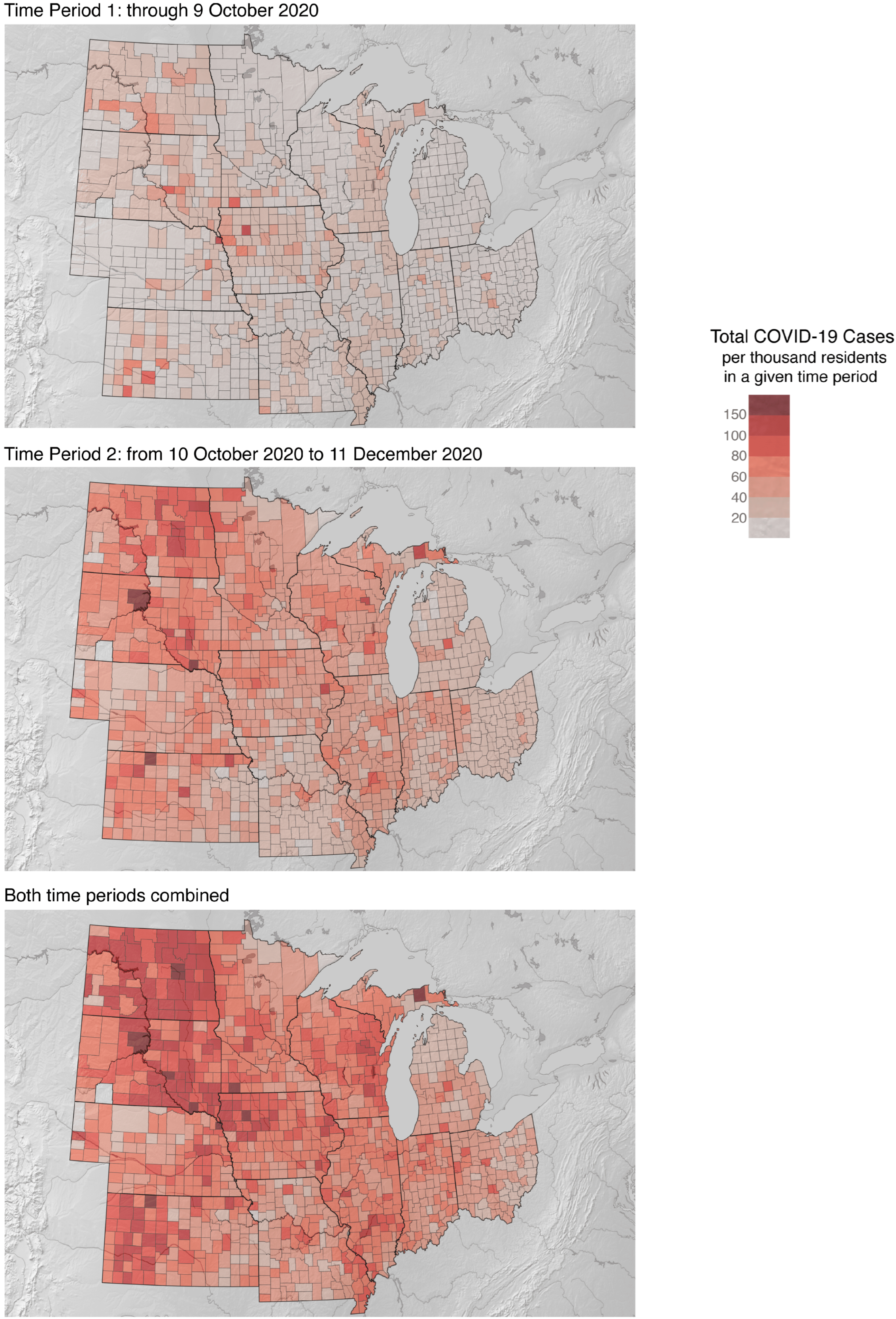
2.2. Choice of Time Periods for Study

We studied the sociospatial dynamics of COVID-19 before any vaccines were authorized for population-level use in the United States. The first such vaccine received Emergency Use Authorization (EUA) on 11 December 2020. We considered the pandemic as having potentially passed through relatively distinct phases of dynamics before that point, which suggested studying any such subperiods separately as well as in the aggregate. We used SaTScan’s method for retrospective space-time cluster detection [24,25] to locate any boundaries between such subperiods. Further details are available in the Supplementary Methods.

2.3. (Global) Linear Regression Models

We began by examining global linear models of county-level cumulative COVID-19 rates in each of the periods we were studying. We did this to understand if some of the disease patterns occurred independently of the explicit consideration of space. For that, we chose ordinary least squares (OLS), given the method assumes independence across observations. If $X_m$ are the various covariates discussed above (and found under the second column of Table S1), and if $X_{mi}$ are the values of the variable $m$ at locations $i$, the set of linear models we fit via OLS has the following form:

$$y_i={\beta }_0+{\displaystyle \sum }_m{\beta }_m{X}_{mi}+{\epsilon }_i$$

(1)

Here, $\epsilon$ represents an independent, identical, and normally distributed error; ${\beta }_m$ are the regression coefficients; and ${\beta }_0$ is an intercept.

We searched the model space of combinations of the possible covariates in Table S1 by using backward elimination to find the model receiving the greatest support from the observed data [26]. This process balances the goodness of fit with model simplicity, i.e., fewer parameters. We began with all potential covariates included in the model. In each ‘step’, we examined whether the model currently under consideration in that step had a fit with a lower Akaike Information Criterion (AIC) than the fits of any of the models that could be formed by dropping a single parameter from the model.

If the current model had the lowest AIC, we examined whether its fit met regression assumptions, and if so, we selected that current model as the best. If, by contrast, we had found one or several models whose fit had lower AIC, we used the simpler model (or if several, the one whose fit had the lowest AIC) as the basis for another iterative step considering what variable might be dropped, until no omitting a single variable from the model would yield a model with a lower AIC.

2.4. (Global) Spatial Econometric Models

In the above modeling approach, the extent to which geography matters is assumed to be captured in the particular combinations of covariates that are observed. However, if there are relations either among errors or among COVID-19 cases such that the values for places that are more ‘sociospatially related’ to each other are autocorrelated, a spatial econometric approach is needed [27,28]. We, therefore, also examined spatial lag and spatial error model formulations, applying a model selection approach not only to consider various combinations of possible covariates (as above) but also simultaneously testing different spatial weights matrices reflecting different combinations of potentially relevant sociospatial relations. We suggest that the methods we develop below offer a quantitative contribution to the relational approach to space and place advocated in health geography [29].

We describe the individual models first, followed by the spatial weights matrices considered, and finally, the model selection process. For spatial lag models,

$$y_i={\beta }_0+{\displaystyle \sum }_m{\beta }_m{X}_{mi}+\rho {\displaystyle \sum }_k{W}_{ki}{y}_k+{\epsilon }_i$$

(2)

where $\rho$ is a parameter to be estimated that reflects the overall strength of the dependence of the dependent variable in a given place on its values in related places, where the relative values of such dependencies are reflected by a spatial weights matrix, $W$. Likewise, for the spatial error model, we model the dependence of error terms arising from their spatial autocorrelation:

$$\begin{array}{c}{y}_i={\beta }_0+{\displaystyle {\displaystyle \sum }_m}{\beta }_m{X}_{mi}+u_i\\ u_i=\lambda {\displaystyle {\displaystyle \sum }_k}{W}_{ki}{u}_k+{\epsilon }_i\end{array}$$

(3)

where ${\epsilon }_i$ are independent and normally distributed; $W_{ki}$ is a spatial weights matrix reflecting spatial interdependence among locations in a manner thus related to, but somewhat different from, the role $W$ plays in the aforementioned spatial lag formulation; and $\lambda$ is an additional parameter to be estimated reflecting the strength and direction of the spatial relationship between terms $u_i$.

Spatial weight matrices are often constructed via one of a small set of standard approaches. Here, we examine whether spatial weights that might be more reflective of the sociospatial processes of COVID-19 epidemiologies yield models whose fits better meet regression assumptions and better explain the observed data [30,31]. In particular, we examine one form of abstract spatial weights, an inverse squared distance matrix, along with two weights matrices that reflect sociospatial processes believed to be of relevance to COVID-19′s spread in the U.S. Midwest: a measure of food trade among counties [32] and a measure of commuting flows between counties [33]. Details of matrix construction are found in Table S1, but we note here that each of these matrices is rendered symmetric via an averaging of bilateral flows and is then row-standardized.

We further allow for the possibility that a combination of the aforementioned types of spatial relations might form a better-fitting model. As such, we also consider all pairwise combinations (A, B) of the aforementioned three basic forms of matrices in linear combinations 0.95 A + 0.05 B and 0.5 A + 0.5 B. Each of these resulting matrices is then row-standardized. This yields a total of 15 spatial weights matrices we examine.

Model selection for either spatial lag or spatial error models then proceeds as follows. For each of the 15 spatial weights matrices in each of the 3 time-period aggregations, we engage in backward elimination of covariates akin to that followed above for global linear models, selecting variables to eliminate, if any, via an AIC criterion while ensuring regression assumptions are met. Then, in each of the 3 time-period aggregations, among the 15 resulting models, each fitted with a different spatial weights matrix, we choose the model fit that minimizes AIC. Our approach thus differs from that of Krisztin et al. [28], who adopt a Bayesian approach but do not consider combinations, and from that of Zhang and Wang [34], who considered multiplicative combinations with additional restrictive assumptions on kernel shape.

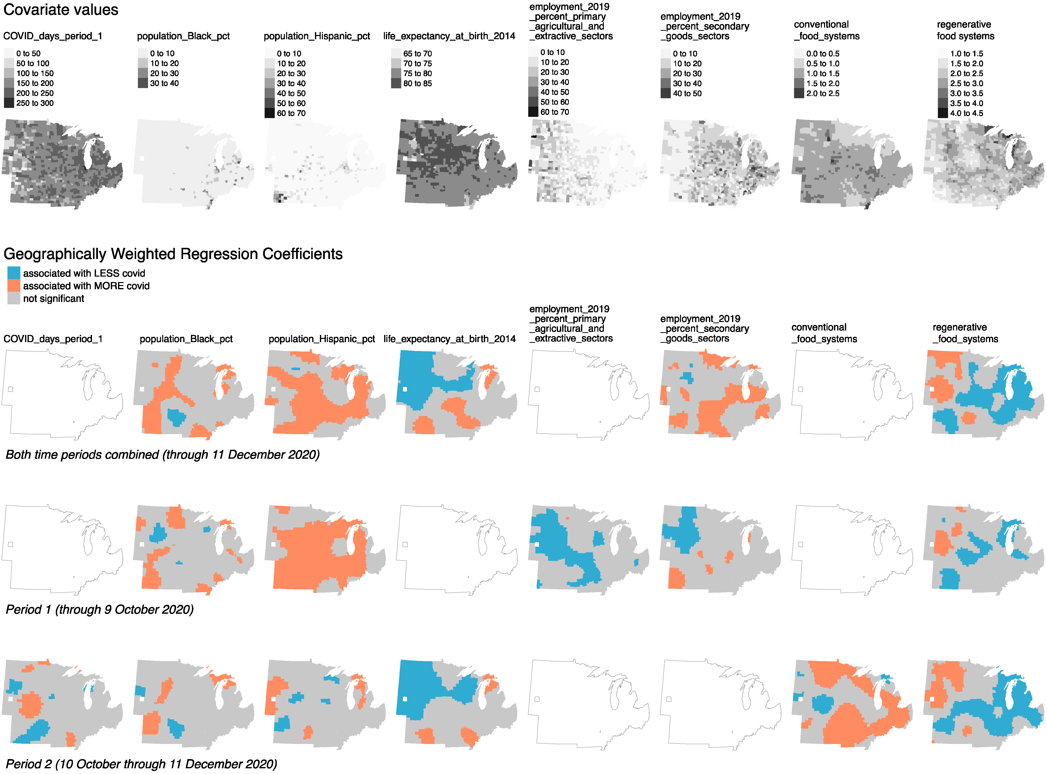
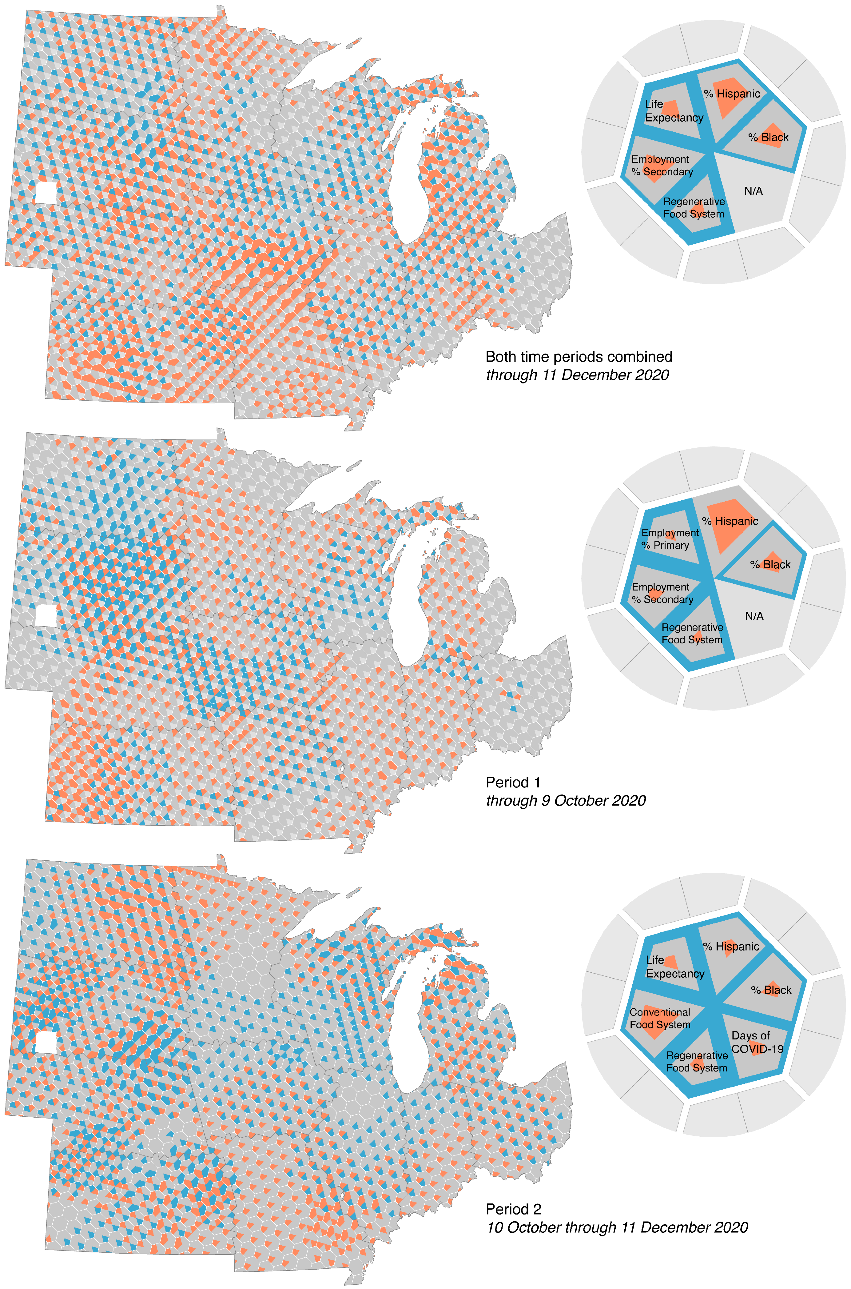
2.5. (Local) Geographically Weighted Regression Models

The global regression approaches used above assume that the same combinations of processes and relations hold across the thousand-plus counties of the U.S. Midwest. Here, we relax this assumption by using a local regression method, Geographically Weighted Regression (GWR), which allows us to examine what different relationships between COVID-19 and our covariates hold in different places, and, if so, what those relationships are [35]. In doing so, we contribute methodologically and empirically to the literature in health and medical geography concerned with the identification of contextual effects and the differences in process between locales [29,36], though we join those who are helping develop methods [37,38] that complement multi-level modeling approaches more typically used in quantitative health geography [39]. Not unlike the global OLS cases, for the local GWR regressions, we have models of the form:

$$y_i={\beta }_0+{\displaystyle \sum }_m{\beta }_m(\overrightarrow{v})X_{mi}+{ϵ}_i(\overrightarrow{v})$$

(4)

with the difference from the OLS cases being that both the regression coefficients ${\beta }_m$ and the error term ${ϵ}_i$ are here functions of $\overrightarrow{v}$, a vector in space measured from the location of the current datapoint $i$. Each point in a GWR regression has its own local weighted regression with its own regression coefficients ${\beta }_m(\overrightarrow{v})$. The regression associated with a given datapoint $i$ is weighted by a Gaussian kernel, $w_j(\overrightarrow{v})$, with:

$$w_j(\overrightarrow{v})=exp\left(-\frac{1}{2} {\left(\frac{d_j(\overrightarrow{v})}{h}\right)}^2\right)$$

(5)

where d_j($\overrightarrow{v}$) is the great circle distance between $i$ and $j$. A characteristic bandwidth, $h$, determines how localized the local regression is and was selected using a cross-validation approach provided by the bw.sel function of the R library GWModel [40]. Models were likewise fit using the GWModel’s gwr.basic function.

In a parallel treatment to our model selection of the best OLS model, we selected our GWR model for a given time period using backward selection via an AICc criterion, choosing the simplest model whose local collinearity diagnostics were also satisfactory. With respect to the latter, we mapped Geographically Weighted correlations between all pairs of covariates and Variance Inflation Factors (VIF) for each of the covariates, where the absolute values of correlations were not to exceed 0.8 on the landscape, and the VIF were less than 10 [40,41].

Finally, instead of solely examining how processes would seem to individually vary over the landscape by separately mapping each resulting fit coefficient ${\beta }_m(\overrightarrow{v})$, we also offer a novel approach to the cartographic visualization of GWR results, which allows readers to identify the extent to which there may be distinct regions on the landscape that emerge from sociospatial processes operating differently in different combinations. To do so, we map all coefficients ${\beta }_m(\overrightarrow{v})$ on a single map, constructing multivariate relational visualizations displaying coefficients within patterns of repeating shapes with different orientations [42]. We thus demonstrate how contemporary spatial analytic methods such as GWR may be used to empirically re-engage longstanding questions in geography around the constitution of regions [43].

3. Results

We interpret the results of our SatSCan analyses as suggesting we not only study COVID-19 incidence over the whole period through the authorization of the first vaccines for emergency use on 11 December 2020, but also study two subperiods. SaTSCan found a temporal cluster over a period from 10 October 2020 to the end of the study on 11 December 2020, which included all the studied counties and had a significant relative risk of 11.16 (LRT= 2,809,322, p < 0.001) when compared with the time before it. We term the time of this cluster ‘Period 2′ and the time before it ‘Period 1′.

Below, studies of Period 1 use the response variable COVID_cases_per_1000persons__over_period_1 which has a summation of COVID cases up until 9 October 2020. Those of ‘period 2′ use the response variable COVID_cases_per_1000persons__over_period_2 for which the cases from 10 October until 11 December 2020 are included. This temporal cluster occurred when there was further spatial COVID-19 case clustering across the northern and western counties of the Midwest (Figure S4). Finally, we model the whole period in 2020 up to 11 December, referring to it as ‘both periods’ as it contains both subperiods 1 and 2 and calling the corresponding variable COVID_cases_per_1000persons__over_both_periods. Figure 1 shows the distribution of COVID-19 per 1000 population over the counties in the different time periods we consider. Distributions of our other variables are plotted in Figure S2.

3.1. Global Generalizations Found by Econometric Models (OLS, Spatial Lag, and Spatial Error Models)

Table 1. Comparison of model fits selected for best explanation of COVID-19 rates over Periods 1, 2, and both periods combined. Pluses (+) and minuses (−) indicate direction of a parameter that is included in selected model. For pluses and minuses, black indicates significance at the 0.05 level; grey indicates not significant. Most GWR results vary over the landscape from positive to negative, as seen below. Those that do are indicated by both a plus and minus (+ −). AIC differences are measured from the model with the lowest AIC for the period. We did not report AIC values for GWR given both that it was fit on 1053, not 1050, counties and that AICc was the relevant measure. Full selected model results are available in Tables S2–S10.

	Global Linear (OLS)			Global Spatial Lag			Global Spatial Error			Local GWR
Time Period ->	1	2	Both	1	2	Both	1	2	Both	1	2	Both
days_of_COVID_period_1	+										+ −
uninsured_pct	+	−	−	+	−			−	−
income_inequality	+		+	+			+
population_Black_pct										+ −	+ −	+ −
population_Hispanic_pct	+	+	+	+	+	+	+		+	+	+ −	+ −
population_Asian_pct		−	−	+	−	−	+	−
population_Native_pct	+	+	+	+	+	+	+	+	+
life_expectancy _at_birth_2014	+	+	+					−	−		+ −	+ −
employment_2019 _percent_primary _agricultural_and _extractive_sectors	−	+		−	−	−	−	−	−	+ −
employment_2019 _percent_secondary _goods_sectors				+	+	+	+	+	+	+ −		+ −
slaughterhouses	+			+		+	+		+
conventional_food_system	+	+	+		+	+	+	+	+		+ −
regenerative_food_system	−	−	−		−	−	−	−	−	+ −	+ −	+ −
W: 0.95 1/Dist2 + 0.05 commute					+	+		+	+
W: 0.95 1/Dist2 + 0.05 foodflows				+			+
AIC above period min	473	476	646	159	26	92	0	0	0	NA	NA	NA

shows the covariates that appeared in the best model found (the Methods section above further explains these variables, with additional detail in Table S1). Positive values for a given variable in the Estimate column indicate that modeled COVID-19 rates per thousand increase with that covariate. By contrast, a negative estimate indicates that modeled COVID-19 rates decrease as such covariates increase their values.

Some of the variables had associations with COVID-19 rates that were similar to each other independently of the modeling assumptions. Central to the concerns of our study, we observed that COVID-19 rates increased with conventional_food_system and decreased with regenerative_food_system, suggesting that dominant modes of agricultural production were important to COVID-19 spread and transmission. Overall, the percentage of the population employed in the primary (agricultural) sector was negatively associated with COVID-19 rates during period 1, a pattern that was also significant in the spatial lag and spatial error models for period 2 and in the best models for both periods. To control for the percentage of jobs within a county that is in the primary sector is to account for how rural the county is, which suggests that it is the model of agricultural production (conventional vs. regenerative/agroecological) that is important to the observed COVID-19 rates.

Further evidence for the role of dominant modes of agricultural production in shaping spread and transmission patterns comes from the examination of variables related to more industrialized activities. Across all econometric models where it appeared, the number of slaughterhouses was positively associated with larger COVID-19 rates. In the spatial error and spatial lag models, for period 2 and both period models, the percent of the population engaged in the secondary sector was positively associated with COVID-19 rates, reinforcing the possibility that activities related to conventional agriculture as a dominant mode of production were key for the spread and exacerbation of COVID-19 transmission.

Patterns of robust association were also observed for some variables quantifying a variety of social variables, including many census concepts of race and ethnicity. For example, counties with higher proportions of Hispanic population had higher COVID-19 rates across most models and studied periods. A similar positive association pattern was observed for the proportion of Native population. However, for Asian population, estimates tended to be negative over both periods, probably reflecting that it was mostly negative for period 2 while being positive for period 1. A different pattern was observed for Black population, which was only selected in the GWR model, which we discuss in the next section. Income inequality tended to be associated with increased COVID-19, especially early in the pandemic. Controlling for these social dimensions, while themselves entwined with more expansive notions of modes of agricultural production—as we see below in regionalizations offered by GWR—accentuates the aforementioned relationships between agriculture and COVID-19.

In terms of variations in the results, some factors were only significant in one but not both of the subperiods, which may indicate a temporal change in COVID-19 epidemiology. In addition to changing relationships between COVID-19 and both inequality and Asian population noted above, days of COVID-19 transmission was only significant for the best Period 1 model using OLS. One understanding of this result is that the relative time of the first arrival of COVID matters less as various temporal waves of the epidemic passed. Yet, when the ‘days of COVID-19 transmission’ variable is presented alongside a variable whose effect differed across the global models we studied, a different perspective emerges. Life expectancy at birth had positive coefficients in the OLS models, was not selected in the spatial lag models, and had negative coefficients for period 2 and both periods in the spatial error models. At the same time, according to our AIC-based model selection, spatial error models were the best for each period (Table 1), and the best spatial weight matrices—while combined with a standard assumption about decreasing association with absolute distance—included food flows for period 1 and commuting patterns for period 2 and both periods.

These results are significant, as they are further validated both by significant likelihood ratio tests comparing these models to OLS models (LR tests presented in Tables S8–S10) for the best models and also by the z-tests for the significance of the spatial matrices (Tables S8–S10). The role of ‘days of COVID transmission’ can thus equally be seen as the abstraction of relational space into time, as it is only significant for the OLS model. The apparent temporal effect may actually be reflecting the relational spaces of food flows, themselves interwoven with the dominant modes of agricultural production, as the latter are better supported by multiple criteria for model selection than using a time covariate. In that sense, the association with life expectancy might be predominantly negative (as supported by the GWR models discussed in the next section).

If so, including relational spaces in the model was important for proper inference. Figures S5 and S6 explore the differences between the more common inverse-squared absolute distance spatial matrices and the mixtures of such matrices with social and agroecological practices we found to be integral to our best models. Multiscalar and urban-rural connections are clearly important to understanding COVID-19′s rural epidemiologies.

3.2. Regions of Stable Epidemiological Process and Their Borderlands

Figure 2 shows key results from the best GWR models for each time period. Each column of the graphic represents a different covariate present in at least one of the models selected by AICc minimization as the best GWR model from that period. Note that only 8 of the 13 covariates considered appear in any of these three best GWR models. The other five variables are not given columns here. The three rows of maps in the GWR coefficient section of the figure each corresponds to the best model at a particular time period. In these maps, orange areas represent counties where a local parameter coefficient is positive and significant, blue represents a local parameter coefficient that is negative and significant, and grey represents a parameter coefficient that is not significant at the 0.05 level. Maps consisting merely of the borders of the region correspond to variables that were present in one of the best models but not in the best model of that row’s time period. Further information on the fitting and selection of these three models can be found in Supplementary Results S1 and Figures S7–S9.

Figure 3 presents much of the information of Figure 2 but does so in a manner that aligns the results together. The mosaic of tiles of covariates allows examining how the relationships the explanatory variables share with cumulative COVID-19 change over space and time, forming emergent regions of distinct epidemiological processes. Given different GWR bandwidths across the runs, stochastic variability, and presumably shifts in pandemic epidemiology over time, it is notable that most covariates that appeared in the best runs of more than one period showed roughly the same patterns across periods (Exceptions include two rapid changes: (1) processes relating the percentage of Hispanic population and COVID-19 rates in period 2 are different than in either period 1 or in both periods together; and (2) more rapid shifts in the roles of employment in the secondary (goods-producing) sector from period 1 to ‘both periods’. We will return to this question of relative process stability below when examining emergent regions across Figure 3).

In terms of social variables, including census concepts of race and ethnicity, there were some notable continuities and differences with the results of the global models presented above. None of the GWR models included percent Asian or percent Native, yet all of them did include percent Black and percent Hispanic, which were mostly positively associated with COVID rates where significant. Positive and significant relationships for percent Hispanic were, aside from Period 2, an extensive phenomenon across much of the Midwest, whereas for percent Black, although there were smaller such areas in the plains, there were also positive associations in regions around the Great Lakes, some of them more urbanized and industrial. Percent Black also had regions of negative association with COVID-19 rates, which may have contributed to the variable not being significant in most global analyses and would likely not have been identified as a noted part of this study’s results without local geographic regressions. In contrast to the global results, inequality was not selected as a significant variable among the best GWR models.

The GWR results suggest the relationships between modes of agricultural production and COVID-19 vary over space. For a swath of counties from Kansas in the southwest of the study area to the Great Lakes (in the northeast of the study area of Figure S1) and down toward the Ohio River (forming much of the southeastern border of the study area), an environment more associated with regenerative agriculture (regenerative_food_system) was itself associated with less COVID-19. Likewise, in many of those areas or nearby, conventional agriculture was associated with more COVID-19. Yet, for much of the more northerly plains, our measure for regenerative agriculture was associated with more COVID-19. Likewise, in those areas, employment in secondary (goods-producing) sectors was often associated with less COVID-19 instead of with more COVID-19, as was elsewhere. Where it was included and significant in Period 1, higher shares of agricultural employment, in general, were negatively associated with COVID-19.

Figure 3 encapsulates the resulting complexity in epidemiological process, under the caveat that while comparing the three time periods is possible, it requires visual care, as not all the variables are shared by best models across time periods. Yet, beginning by examining each time period separately, areas of process stability are visible where particular combinations of variables are related positively, negatively, and non-significantly to COVID-19.

For example, much of the states of Indiana and Illinois lie within one region of epidemiological process in Period 1 and ‘both periods’. Percent Hispanic is positively associated with COVID-19 across the two states and the two periods, even as regenerative farming is protective only when considering ‘both periods’. Other variables, such as those around employment structure, become significant as one moves westward into Iowa and Missouri, and fewer variables are significant eastward into Ohio.

In another example, the various subregions within North Dakota, South Dakota, and Nebraska host their own socioecology, most clearly differentiated from those of Minnesota in Periods 1 and 2 along their border. Often, fewer and different variables are significant in Minnesota than across the Dakotas. As seen in Figure 2, these plains states have relatively unique combinations of processes related to COVID-19, compared to much of Kansas, Iowa, and Minnesota, where, among other processual differences, regenerative agriculture was generally associated with less COVID-19.

4. Discussion

4.1. U.S. Midwest COVID-19 and Modes of Agricultural Production

Our results suggest initial COVID-19 spread in the U.S. Midwest can be characterized not only through more commonly discussed factors of health, demography, and behavior but also through the lens of counties’ dominant modes of agricultural production. “Conventional” and “regenerative” agricultural modes of production differ in the extent to which production is entrained in the dynamics of larger capitalist economic formations and the extent to which each tends to reproduce local social and ecological relations. Although these modes of agricultural production are abstractions, we can locate suitable indicators of their expression, as we have from Bergmann et al. [18]. Future research would benefit from devising indices that more directly quantify relevant relations of labor, property ownership, and the absolute and relational spatialities of landscape. Yet, in using available metrics, we found here that across the U.S. Midwest, regenerative agricultural landscapes were generally protective against COVID-19, while conventional agricultural landscapes were associated with more COVID-19 cases per capita.

There are many possible causes. On the one hand, counties hosting greater regenerative production may be peripheral to major supply lines of industrial agricultural production. The latter networks connect what may be, in other senses, ‘distant’ counties into regional livestock outbreaks or—for pathogens that have already spilled over into human populations—urbanized pandemics [32,44,45,46]. Chaves et al. [47] showed that moderating certain sorts of international interconnection (whether by strategic ‘delinking’ [48] or unwanted peripheralization [49,50]) reduced the burden of COVID-19 in countries of Mesoamerica and the Caribbean.

In combination with such highly connected sites in the U.S. Midwest, agricultural occupational risk appears to shape patterns of COVID-19 spread. Taylor et al. [6] associated excess COVID-19 cases and deaths as of July 2020 with proximity to livestock processing plants. The team estimated 236,000 to 310,000 cases and 4300 to 5200 deaths from plant-associated outbreaks, with the vast majority of cases and deaths from community spread beyond the plants. The larger community outbreaks were associated with larger processing facilities and larger meatpacking companies. Taylor et al. [6] found plant closures attenuated county caseloads, while plants that received USDA permission to stay open and increase line speeds were associated with more countywide cases.

Protection at the county level may extend beyond merely being disconnected from documented COVID-19 conduits. Mechanisms might be multiple and benefit from ethnographic case study. In Italy, farmers engaged in more regenerative counties engaging (no-contact) local sales survived and even profited during the worst of the early phases of the pandemic [51]. Innovations in online sales, farm stops, sponsor-a-neighbor programs, and neighborhood ‘drop spots’ embody flexibility that smallholder operations have long demonstrated in crises [52,53,54]. Although regenerative farming regions are not synonymous with community adherence to public health protections, and many conventional agricultural counties also prospered during the pandemic, regenerative counties whose farmers succeeded together as a community of producers under such duress may be in a better position to supply local nutrition and sustain the community trust associated with healthier outcomes [55].

As our geographically weighted regression model shows, however, such sweeping associations are likely context-specific [36]. The devaluation, unabsorbed overaccumulation, and, from capital’s vantage, underconsumption that COVID-19 outbreaks imposed were felt in uneven fashion across industrial Midwest operations [56,57]. Some agricultural markets were directly hit by outbreaks, others only farther along their value chains, and some none at all. The impacts and responses were also actively produced. With state intervention, conventional agriculture stateside—particularly consolidated suppliers and buyers that may have been the proximate source of rural outbreaks—survived and even prospered, whatever the damage to individual farms, food workers, or the people living in a plant’s county [54,58]. Sudden disruptions, including a pandemic producing a million deaths in the US, can lead to new processes of accumulation in productive commodity frontiers [59,60,61].

Regenerative counties also differ in the details of their modes of social reproduction. Which pandemic-specific innovations work where is conditional. Did Community-Supported Agriculture programs work best in rural counties nearer to urban consumer markets? Were counties farther afield from cities and industrial meatpackers both more likely to return to agricultural business-as-usual? Were such returns still dependent upon how the county’s distal supply lines and end buyers were affected by the pandemic? To what extent did on-farm labor’s working conditions, compensation, housing, and social vulnerability impact pandemic safety in even these ostensibly remote counties? These and other questions of deepening complexity bear further investigation.

4.2. Social Relations and Processes in U.S. Midwest COVID-19

Alongside local agricultural practices, other historical and geographical aspects of society proved important to COVID-19. Early rural COVID-19 outcomes were socially structured, including by poverty and underlying health [4,6,62,63]. Using spatial autoregressive models, Fielding-Miller et al. [4] showed that along with residents living in poverty, density, population size, and residents over the age of 65, COVID-19 mortality by July 2020 was also positively associated with a county’s percent of farmworkers.

Race also marked differences in rural COVID-19 exposure. Cheng et al. [64] showed through July 2020, rural counties in the top quartiles of Black and Latino populations hosted 70% and 50% percent greater average daily COVID-19 increases, respectively, than counties in the lowest quartiles. Lundberg et al. [65] found Black and Latino populations with the highest COVID-19 death rates across U.S. regions and urban and rural settings. The disparity was worst in the first year of the pandemic, but even upon vaccination held in place the second year, when white mortality increased or, as in the Midwest, held steady. As many of our models here underscored, the percentages of non-white populations repeatedly were associated with higher COVID-19 caseload. Although census-reported Black population proved an insignificant covariate in the global econometric models, once considering local variations of process over space, the geographically weighted regressions identified diverse regional relationships between Black populations and cases.

McClure et al. [66] connected such disparities to a racial capitalism that uses Black and immigrant labor—in parts of the Midwest and beyond—to allow a whiter and wealthier professional class to shelter-in-place during a pandemic. In our results above, where the model selection process dropped consideration of the percentage of the population that is Black, it often nonetheless retained measures of income inequity, which, as noted, are understood within the ongoing historical context of the U.S. to be complexly interrelated with race.

Our methods show contingencies in relations between race, COVID-19, and other variables as well. While percentage Hispanic repeatedly proved positively associated with cumulative COVID across time periods, perhaps linked to some of the most dangerous agricultural working conditions, the combinations of other factors with which it was associated shifted across the Midwest (Figure 3). For instance, in Period 1 throughout Michigan, cumulative COVID-19 appeared associated solely with percent Hispanic, while across large parts of South Dakota, it was also linked with (positively associated with COVID) regenerative production as well as (negatively associated with COVID) percent Black, percent employment in the primary sector, and percent employment in the secondary sector.

A limitation of this study arises from socio-spatial determinants of health operating at other scales than that of the county. Our methods were able to capture some of those as embodied within county-level measures, such as those reflective of agricultural modes of production. Others were captured through our attention to spatial relations. However, our methods were not multi-level and, thus, were less able to directly study the effects of, e.g., state-level COVID policies or longer-standing state-level health differences. Yet, to the extent that state-level differences were to have had strong effects on the geographies of COVID, we might have expected visible border effects in Figure 3, where few appear upon visual inspection. Nonetheless, future research would benefit from multi-level spatial econometric and GWR methods.

5. Conclusions and Beyond: Contextual Method and Collective Solutions

Through helping develop quantitative methods that are sensitive to context and relation, we hope to have contributed to efforts in health geography, epidemiology, and cognate fields that seek to support social change and well-being across a variety of scales. Public and non-governmental actors can take up the approaches advocated to better tailor the scales of their policies and engagements to the scales of the phenomena (here, COVID-19 spread) that emerge from the processes and relations of the integrated system under study itself. Those that seek to learn from the successful experiences of others have additional tools to examine whether the contexts from which they are learning differ from their own, and if so, they may inform themselves better how to learn and collaborate across difference.

While we lament that quantitative efforts have often diverged in topics, assumptions, and approaches from more qualitative research despite a widespread desire to move past false dichotomies and divide [67], we believe that a synthetic approach to topics (here, at the intersection of food systems, health geography, ecology, and political economy) using a carefully curated set of quantitative methods may contribute to closing these divides. Extending the research pursued above, multi-sited qualitative (perhaps even ethnographic) research would be useful in triangulating our highly context-specific and relational results.

In the situations we are specifically examining here, we recognize the urgency that some such research be participatory action research, contributing to a possible shift in the food systems in the US Midwest and beyond [53]. Disruptions to just-in-time large-scale agricultural production have led to new efforts at re-establishing local meat processing plants [68,69]. These and other initiatives may serve to help re-establish virtuous cycles across modes of agricultural production, ecological services, and community well-being [70]. By helping reintroduce agrobiodiversity and economic complementarity, these efforts, as the results reported here suggest, may be beneficial to community health, perhaps even beyond the case examined here, as novel diseases and health challenges arise.

References

1. Lytras, S.; Hughes, J.; Martin, D.; Swanepoel, P.; de Klerk, A.; Lourens, R.; Kosakovsky Pond, S.L.; Xia, W.; Jiang, X.; Robertson, D.L. Exploring the Natural Origins of SARS-CoV-2 in the Light of Recombination. Genome. Biol. Evol. 2022, 14, evac018. [Google Scholar] [CrossRef] [PubMed]
2. Pekar, J.E.; Magee, A.; Parker, E.; Moshiri, N.; Izhikevich, K.; Havens, J.L.; Gangavarapu, K.; Serrano, L.M.M.; Crits-Christoph, A.; Matteson, N.L.; et al. The Molecular Epidemiology of Multiple Zoonotic Origins of SARS-CoV-2. Science 2022, 377, 960–966. [Google Scholar] [CrossRef] [PubMed]
3. Belanger, M.J.; Hill, M.A.; Angelidi, A.M.; Dalamaga, M.; Sowers, J.R.; Mantzoros, C.S. COVID-19 and Disparities in Nutrition and Obesity. N. Engl. J. Med. 2020, 383, e69. [Google Scholar] [CrossRef] [PubMed]
4. Fielding-Miller, R.K.; Sundaram, M.E.; Brouwer, K. Social determinants of COVID-19 mortality at the county level. PLoS ONE 2020, 15, e0240151. [Google Scholar] [CrossRef]
5. Lusk, J.L.; Chandra, R. Farmer and farm worker illnesses and deaths from COVID-19 and impacts on agricultural output. PLoS ONE 2021, 16, e0250621. [Google Scholar] [CrossRef] [PubMed]
6. Taylor, C.A.; Boulos, C.; Almond, D. Livestock plants and COVID-19 transmission. Proc. Natl. Acad. Sci. USA 2020, 117, 31706–31715. [Google Scholar] [CrossRef]
7. van der Ploeg, J.D. From biomedical to politico-economic crisis: The food system in times of COVID-19. J. Peasant Stud. 2020, 47, 944–972. [Google Scholar] [CrossRef]
8. Griffith, D.; Li, B. Spatial-temporal modeling of initial COVID-19 diffusion: The cases of the Chinese Mainland and Conterminous United States. Geo.-Spat. Inf. Sci. 2021, 24, 340–362. [Google Scholar] [CrossRef]
9. Wang, Y.; Liu, Y.; Struthers, J.; Lian, M. Spatiotemporal Characteristics of the COVID-19 Epidemic in the United States. Clin. Infect. Dis. 2020, 72, 643–651. [Google Scholar] [CrossRef]
10. Albrecht, D.E. COVID-19 in Rural America: Impacts of Politics and Disadvantage*. Rural. Sociol. 2022, 87, 94–118. [Google Scholar] [CrossRef]
11. Sun, F.; Matthews, S.A.; Yang, T.-C.; Hu, M.-H. A spatial analysis of the COVID-19 period prevalence in US counties through June 28, 2020: Where geography matters? Ann. Epidemiol. 2020, 52, 54–59.e51. [Google Scholar] [CrossRef] [PubMed]
12. Ridenhour, B.J.; Sarathchandra, D.; Seamon, E.; Brown, H.; Leung, F.-Y.; Johnson-Leon, M.; Megheib, M.; Miller, C.R.; Johnson-Leung, J. Effects of trust, risk perception, and health behavior on COVID-19 disease burden: Evidence from a multi-state US survey. PLoS ONE 2022, 17, e0268302. [Google Scholar] [CrossRef] [PubMed]
13. Souch, J.M.; Cossman, J.S. A commentary on rural-urban disparities in COVID-19 testing rates per 100,000 and risk factors. J. Rural. Health 2021, 37, 188. [Google Scholar] [CrossRef]
14. Cuadros, D.F.; Branscum, A.J.; Mukandavire, Z.; Miller, F.D.; MacKinnon, N. Dynamics of the COVID-19 epidemic in urban and rural areas in the United States. Ann. Epidemiol. 2021, 59, 16–20. [Google Scholar] [CrossRef]
15. Murphy, P.J. Unlocking the Means of COVID-19 Spread From Prisons to Outside Populations. Am. J. Public Health 2021, 111, 1392–1394. [Google Scholar] [CrossRef] [PubMed]
16. Amin, S. Modes of Production, History and unequal development. Sci. Soc. 1985, 49, 194–207. [Google Scholar]
17. Amin, S. Modes of Production and Social Formations. Ufahamu J. Afr. Stud. 1974, 4, 57–85. [Google Scholar] [CrossRef]
18. Bergmann, L.; Chaves, L.F.; Betz, C.R.; Stein, S.; Wiedenfeld, B.; Wolf, A.; Wallace, R.G. Mapping Agricultural Lands: From Conventional to Regenerative. Land 2022, 11, 437. [Google Scholar] [CrossRef]
19. Li, C.; Hoffland, E.; Kuyper, T.W.; Yu, Y.; Zhang, C.; Li, H.; Zhang, F.; van der Werf, W. Syndromes of production in intercropping impact yield gains. Nat. Plants 2020, 6, 653–660. [Google Scholar] [CrossRef]
20. Cusworth, G.; Dodsworth, J. Using the ‘good farmer’concept to explore agricultural attitudes to the provision of public goods. A case study of participants in an English agri-environment scheme. Agric. Hum. Values 2021, 38, 929–941. [Google Scholar] [CrossRef]
21. Paul, R.; Arif, A.; Pokhrel, K.; Ghosh, S. The association of social determinants of health with COVID-19 mortality in rural and urban counties. J. Rural. Health 2021, 37, 278–286. [Google Scholar] [CrossRef] [PubMed]
22. New York Times. Coronavirus (COVID-19) Data in the United States for 2020. Available online: https://github.com/FoldingSpace/COVID-19-data/raw/master/us-counties-2020.csv (accessed on 31 May 2021).
23. U.S. Census Bureau. 2016–2020 American Community Survey 5-Year Public Use Microdata Samples. Available online: https://www.census.gov/newsroom/press-kits/2021/acs-5-year.html (accessed on 1 November 2021).
24. Kulldorff, M. A spatial scan statistic. Commun. Stat. Theory Methods 1997, 26, 1481–1496. [Google Scholar] [CrossRef]
25. Kulldorff, M.; Information Management Services Inc. SaTScanTM v8.0: Software for the Spatial and Space-Time Scan Statistics. Available online: http://www.satscan.org/ (accessed on 5 May 2021).
26. Faraway, J.J. Linear Models with R; CRC Press: Boca Raton, FL, USA, 2004. [Google Scholar]
27. Anselin, L.; Florax, R.; Rey, S.J. Advances in Spatial Econometrics: Methodology, Tools and Applications; Springer: Berlin, Germany, 2013. [Google Scholar]
28. Krisztin, T.; Piribauer, P.; Wögerer, M. The spatial econometrics of the coronavirus pandemic. Lett. Spat. Resour. 2020, 13, 209–218. [Google Scholar] [CrossRef] [PubMed]
29. Prior, L.; Manley, D.; Sabel, C.E. Biosocial health geography: New ‘exposomic’geographies of health and place. Prog. Hum. Geogr. 2019, 43, 531–552. [Google Scholar] [CrossRef]
30. Getis, A. Spatial weights matrices. Geogr. Anal. 2009, 41, 404–410. [Google Scholar] [CrossRef]
31. Lu, B.; Charlton, M.; Brunsdon, C.; Harris, P. The Minkowski approach for choosing the distance metric in geographically weighted regression. Int. J. Geogr. Inf. Sci. 2016, 30, 351–368. [Google Scholar] [CrossRef]
32. Lin, X.; Ruess, P.J.; Marston, L.; Konar, M. Food flows between counties in the United States. Environ. Res. Lett. 2019, 14, 084011. [Google Scholar] [CrossRef]
33. U.S. Census Bureau. Table 1. Residence County to Workplace County Commuting Flows for the United States and Puerto Rico Sorted by Residence Geography: 5-Year ACS, 2011–2015. Available online: https://www.census.gov/data/tables/2015/demo/metro-micro/commuting-flows-2015.html (accessed on 1 November 2021).
34. Zhang, H.; Wang, X. Combined asymmetric spatial weights matrix with application to housing prices. J. Appl. Stat. 2017, 44, 2337–2353. [Google Scholar] [CrossRef]
35. Fotheringham, A.S.; Brunsdon, C.; Charlton, M. Geographically Weighted Regression: The Analysis of Spatially Varying Relationships; John Wiley & Sons: Hoboken, NJ, USA, 2003. [Google Scholar]
36. Kestens, Y.; Wasfi, R.; Naud, A.; Chaix, B. “Contextualizing context”: Reconciling environmental exposures, social networks, and location preferences in health research. Curr. Environ. Health Rep. 2017, 4, 51–60. [Google Scholar] [CrossRef]
37. Forati, A.M.; Ghose, R.; Mantsch, J.R. Examining opioid overdose deaths across communities defined by racial composition: A multiscale geographically weighted regression approach. J. Urban Health 2021, 98, 551–562. [Google Scholar] [CrossRef]
38. He, Y.; Seminara, P.J.; Huang, X.; Yang, D.; Fang, F.; Song, C. Geospatial Modeling of Health, Socioeconomic, Demographic, and Environmental Factors with COVID-19 Incidence Rate in Arkansas, US. ISPRS Int. J. Geoinf. 2023, 12, 45. [Google Scholar] [CrossRef]
39. Owen, G.; Harris, R.; Jones, K. Under examination: Multilevel models, geography and health research. Prog. Hum. Geogr. 2016, 40, 394–412. [Google Scholar] [CrossRef]
40. Lu, B.; Harris, P.; Charlton, M.; Brunsdon, C. The GWmodel R package: Further topics for exploring spatial heterogeneity using geographically weighted models. Geo. Spat. Inf. Sci. 2014, 17, 85–101. [Google Scholar] [CrossRef]
41. Comber, A.; Brunsdon, C.; Charlton, M.; Dong, G.; Harris, R.; Lu, B.; Lü, Y.; Murakami, D.; Nakaya, T.; Wang, Y.; et al. A Route Map for Successful Applications of Geographically Weighted Regression. Geogr.l Anal. 2023, 55, 155–178. [Google Scholar] [CrossRef]
42. Bergmann, L.; O’Sullivan, D. Colorweaver. 2023; manuscript in preparation. [Google Scholar]
43. Hartshorne, R. Perspective on the Nature of Geography; Rand McNally: Chicago, CA, USA, 1959; p. 201. [Google Scholar]
44. Wallace, R.G.; Liebman, A.; Chaves, L.F.; Wallace, R. COVID-19 and Circuits of Capital. Month Rev. 2020, 72, 1–15. [Google Scholar] [CrossRef]
45. VanderWaal, K.; Paploski, I.A.D.; Makau, D.N.; Corzo, C.A. Contrasting animal movement and spatial connectivity networks in shaping transmission pathways of a genetically diverse virus. Prev. Vet. Med. 2020, 178, 104977. [Google Scholar] [CrossRef]
46. Hu, D.; Cheng, T.-Y.; Morris, P.; Zimmerman, J.; Wang, C. Active regional surveillance for early detection of exotic/emerging pathogens of swine: A comparison of statistical methods for farm selection. Prev. Vet. Med. 2021, 187, 105233. [Google Scholar] [CrossRef]
47. Chaves, L.F.; Friberg, M.D.; Hurtado, L.A.; Marín Rodríguez, R.; O’Sullivan, D.; Bergmann, L.R. Trade, uneven development and people in motion: Used territories and the initial spread of COVID-19 in Mesoamerica and the Caribbean. Soc. Econ. Plan Sci. 2022, 76, 101161. [Google Scholar] [CrossRef]
48. Amin, S. A Note on the Concept of Delinking. Review 1987, 10, 435–444. [Google Scholar]
49. Santos, M. The Return of the Territory. In Milton Santos: A Pioneer in Critical Geography from the Global South; Melgaço, L., Prouse, C., Eds.; Springer International Publishing: Cham, Germany, 2017; pp. 25–31. [Google Scholar]
50. Santos, M. Por Uma Outra Globalização: Do Pensamento Único à Consciência Universal; Record: Rio de Janeiro, Brazil, 2000. [Google Scholar]
51. Mastronardi, L.; Cavallo, A.; Romagnoli, L. How did Italian diversified farms tackle COVID-19 pandemic first wave challenges? Soc. Econ. Plan Sci. 2022, 82, 101096. [Google Scholar] [CrossRef]
52. Mann, S.A.; Dickinson, J.M. Obstacles to the development of a capitalist agriculture. J. Peas. Stud. 1978, 5, 466–481. [Google Scholar] [CrossRef]
53. Robinson, J.M.; Mzali, L.; Knudsen, D.; Farmer, J.; Spiewak, R.; Suttles, S.; Burris, M.; Shattuck, A.; Valliant, J.; Babb, A. Food after the COVID-19 pandemic and the case for change posed by alternative food: A case study of the American Midwest. Glob. Sust. 2021, 4, e6. [Google Scholar] [CrossRef]
54. Wallace, R.G. Dead Epidemiologists: On the Origins of COVID-19; Monthly Review Press: New York, NY, USA, 2020. [Google Scholar]
55. Lenton, T.M.; Boulton, C.A.; Scheffer, M. Resilience of countries to COVID-19 correlated with trust. Sci. Rep. 2022, 12, 75. [Google Scholar] [CrossRef] [PubMed]
56. Clapp, J.; Moseley, W.G. This food crisis is different: COVID-19 and the fragility of the neoliberal food security order. J. Peas. Stud. 2020, 47, 1393–1417. [Google Scholar] [CrossRef]
57. Carrillo, I.R.; Ipsen, A. Worksites as Sacrifice Zones: Structural Precarity and COVID-19 in U.S. Meatpacking. Sociol Persp. 2021, 64, 726–746. [Google Scholar] [CrossRef]
58. Wallace, R.G. Big Farms Make Big Flu: Dispatches on Influenza, Agribusiness, and the Nature of Science; Monthly Review Press: New York, NY, USA, 2016. [Google Scholar]
59. Harvey, D. The Limits to Capital; Verso Books: London, UK, 2018. [Google Scholar]
60. Banaji, J. Theory as History: Essays on Modes of Production and Exploitation; Brill: Leiden, The Netherlands, 2010. [Google Scholar]
61. Chaves, L.F. The Dynamics of Latifundia Formation. PLoS ONE 2013, 8, e82863. [Google Scholar] [CrossRef]
62. Tian, T.; Zhang, J.; Hu, L.; Jiang, Y.; Duan, C.; Li, Z.; Wang, X.; Zhang, H. Risk factors associated with mortality of COVID-19 in 3125 counties of the United States. Inf. Dis. Povert. 2021, 10, 1–8. [Google Scholar] [CrossRef]
63. Akinwumiju, A.S.; Oluwafemi, O.; Mohammed, Y.D.; Mobolaji, J.W. Geospatial evaluation of COVID-19 mortality: Influence of socio-economic status and underlying health conditions in contiguous USA. Appl. Geogr. 2022, 141, 102671. [Google Scholar] [CrossRef]
64. Cheng, K.J.G.; Sun, Y.; Monnat, S.M. COVID-19 Death Rates Are Higher in Rural Counties With Larger Shares of Blacks and Hispanics. J. Rural. Health 2020, 36, 602–608. [Google Scholar] [CrossRef]
65. Lundberg, D.J.; Cho, A.; Raquib, R.; Nsoesie, E.O.; Wrigley-Field, E.; Stokes, A.C. Geographic and Temporal Patterns in COVID-19 Mortality by Race and Ethnicity in the United States from March 2020 to February 2022. medRxiv 2022. [Google Scholar]
66. McClure, E.S.; Vasudevan, P.; Bailey, Z.; Patel, S.; Robinson, W.R. Racial capitalism within public health—How occupational settings drive COVID-19 disparities. Am. J. Epid. 2020, 189, 1244–1253. [Google Scholar] [CrossRef]
67. Rosenberg, M. Health geography II: ‘Dividing’health geography. Prog. Hum. Geogr. 2016, 40, 546–554. [Google Scholar] [CrossRef]
68. Thilmany, D.; Canales, E.; Low, S.A.; Boys, K. Local food supply chain dynamics and resilience during COVID-19. App. Econ. Persp. Pol. 2021, 43, 86–104. [Google Scholar] [CrossRef]
69. Pitt, D. USDA Unveils Plan to Help Build Small Meat Processing Plants. Available online: https://apnews.com/article/joe-biden-business-health-coronavirus-pandemic-meat-processing-ca27a1c8c38a1b83c7dbea7620d7b24f (accessed on 9 November 2022).
70. Frison, E.A.; IPES-Food. From Uniformity to Diversity: A Paradigm Shift from Industrial Agriculture to Diversified Agroecological Systems; IPES: Louvain-la-Neuve, Belgium, 2016; p. 96. [Google Scholar]
71. Manson, S.; Schroeder, J.; Van Riper, D.; Kugler, T.; Ruggles, S. IPUMS National Historical Geographic Information System: Version 16.0 2020 Centers of Population; IPUMS: Minneapolis, MN, USA, 2021. [Google Scholar]
72. Kulldorff, M.; Huang, L.; Pickle, L.; Duczmal, L. An elliptic spatial scan statistic. Stat. Med. 2006, 25, 3929–3943. [Google Scholar] [CrossRef] [PubMed]
73. Walker, K.; Herman, M. Tidycensus: Load US Census Boundary and Attribute Data as ‘Tidyverse’ and ‘sf’-Ready Data Frames. Available online: https://walker-data.com/tidycensus/ (accessed on 1 November 2022).
74. U.S. Census Bureau. Small Area Health Insurance Estimates (SAHIE). Available online: https://www.census.gov/content/census/en/data/datasets/time-series/demo/sahie/estimates-acs.html (accessed on 1 November 2022).
75. Dwyer-Lindgren, L.; Bertozzi-Villa, A.; Stubbs, R.W.; Morozoff, C.; Mackenbach, J.P.; van Lenthe, F.J.; Mokdad, A.H.; Murray, C.J.L. Inequalities in Life Expectancy Among US Counties, 1980 to 2014: Temporal Trends and Key Drivers. JAMA Int. Med. 2017, 177, 1003–1011. [Google Scholar] [CrossRef] [PubMed]
76. Institute for Health Metrics and Evaluation. United States Life Expectancy and Age-Specific Mortality Risk by County 1980–2014. Available online: https://ghdx.healthdata.org/record/ihme-data/united-states-life-expectancy-and-age-specific-mortality-risk-county-1980-2014 (accessed on 1 November 2022).
77. U.S. Bureau of Economic Analysis. Personal Income (State and Local), CAEMP25N (Total Full-Time and Part-Time Employment by NAICS Industry), 2001–2020. Available online: https://apps.bea.gov/regional/downloadzip.cfm (accessed on 1 November 2022).
78. United States Department of Agriculture. Food Safety and Inspection Services. Meat, Poultry and Egg Product Inspection Directory. Available online: https://www.fsis.usda.gov/inspection/establishments/meat-poultry-and-egg-product-inspection-directory. (accessed on 11 October 2020).
79. Roth, J. County Distance Database. Available online: https://data.nber.org/data/county-distance-database.html (accessed on 15 February 2022).
80. Ellis, E.C.; Gauthier, N.; Klein Goldewijk, K.; Bliege Bird, R.; Boivin, N.; Díaz, S.; Fuller, D.Q.; Gill, J.L.; Kaplan, J.O.; Kingston, N.; et al. People have shaped most of terrestrial nature for at least 12,000 years. Proc. Nat. Acad. Sci. USA 2021, 118, e2023483118. [Google Scholar] [CrossRef] [PubMed]
Figure 1. Cumulative COVID-19 cases per 1000 population in each of the study time periods. See also Figure S1 for guidance about the US state and county names.
Ijgi 12 00195 g001
Figure 2. Maps of covariate coefficient direction and significance in the best Geographically Weighted Regression models for Periods 1 and 2 and their combination. Each time period has its own row of GWR coefficient maps. Eight different covariates appear in various models for the periods selected by AICc minimization, each corresponding with a separate column. Those variables present in one period’s model but not selected for a given period are represented by blank outlines of the study region. Maps of GWR coefficients show direction and significance. Where counties are colored orange, the covariate in question is positively and significantly associated with more cumulative COVID-19 per thousand residents. Where counties are colored blue, the covariate is negatively and significantly associated with COVID-19. Each selected covariate’s observed distributions are plotted in greyscale maps at the top of the figure. Descriptions of all these variables can be found in Table S1.
Ijgi 12 00195 g002
Figure 3. Relational mapping of geographically weighted regression coefficients and significance over the three periods of the study. The information presented here is also present in Figure 2; however, in this format, it becomes possible to see the emergence of regions with particular COVID-19 epidemiologies. As before, orange represents significantly positive relationships with COVID-19; blue indicates significantly negative relationships; and medium grey indicates the variable is not significant in that county. Legends indicate overall distributions between these categories for each variable.
Ijgi 12 00195 g003