Spatiotemporal Distribution and Influencing Factors of Theft during the Pre-COVID-19 and COVID-19 Periods: A Case Study of Haining City, Zhejiang, China

Abstract

Theft is an inevitable problem in the context of urbanization and poses a challenge to people’s lives and social stability. The study of theft and criminal behavior using spatiotemporal, big, demographic, and neighborhood data is important for guiding security prevention and control. In this study, we analyzed the theft frequency and location characteristics of the study area through mathematical statistics and hot spot analysis methods to discover the spatiotemporal divergence characteristics of theft in the study area during the pre-COVID-19 and COVID-19 periods. We detected the spatial variation pattern of the regression coefficients of the local areas of thefts in Haining City by modeling the influencing factors using the geographically weighted regression (GWR) analysis method. The results explained the relationship between theft and the influencing factors and showed that the regression coefficients had both positive and negative values in the pre-COVID-19 and COVID-19 periods, indicating that the spatial distribution of theft in urban areas of Haining City was not smooth. Factors related to life and work indicated densely populated areas had increased theft, and theft was negatively correlated with factors related to COVID-19. The other influencing factors were different in terms of their spatial distributions. Therefore, in terms of police prevention and control, video surveillance and police patrols need to be deployed in a focused manner to increase their inhibiting effect on theft according to the different effects of influencing factors during the pre-COVID-19 and COVID-19 periods.

1. Introduction

As urbanization accelerates, an increasing number of people are moving to cities, leading to the problem of urban crime becoming increasingly prominent. The occurrence of COVID-19 in recent years has had a significant impact on urban development. Criminal behavior not only disturbs the social order but also seriously threatens people’s daily lives, personal lives, and property safety, which affects the prosperity and stability of society. Crime is a particular human phenomenon, and as such, it has a chronological occurrence, development process, and obvious geographic distribution characteristics.

In 1986, Zhu Xiaoguang [1] proposed the concept of crime geography for the first time in China, which is defined as the science of studying the spatial, occurrence, and distribution laws of the current situation of crime. Foreign research on crime geography is ahead of research in China, and its progress has established the foundation of the development of crime geography in China.

Many scholars have studied the social environment and geographic distribution related to crime geography [2,3,4,5,6,7]. Schweitzer et al. [8] analyzed the relationship between the built environment and crime rates in urban residential areas and found that a sense of community was important in predicting fear of crime. Boessen et al. [9] studied the extent of socioecological influences on crime at the micro scale of neighborhoods and found that accounting for multiple scales simultaneously was important in ecological studies of crime. Mao Yuanyuan et al. [10] used a combination of analytical methods to study the relationship between the spatial distribution characteristics of crime and environmental factors, and their results can facilitate crime prevention through urban planning. Zhou Suhong et al. [11] studied the impact of land use on street robbery cases and suggested that correlative land use planning guidelines be made to consciously prevent the occurrence of criminal behavior. The impact of urban facilities on crimes during the pre-COVID-19 and COVID-19 periods was analyzed independently using negative binomial regression (NBR) and geographical weight regression (GWR) [12].

Since the outbreak of COVID-19, many scholars have conducted numerous studies on the impact of COVID-19 on crime. Prevention and control measures had a significant inhibitory effect on crime and significantly reduced the number of crimes [13,14,15]. Nivette et al. collected data on daily counts of crime in 27 cities across 23 countries in the Americas, Europe, the Middle East, and Asia. Stay-at-home policies were associated with a considerable drop in urban crime, but with substantial variation across cities and types of crime [16]. Ashby analyzed crimes in 16 large cities across the United States in the early months of 2020, and the results were different for different types of crimes, such as residential burglary, non-residential burglary, and thefts from motor vehicles [17].

In recent studies, researchers have started to include social and economic variables to interpret the spatial distribution of crime variations during the COVID-19 period. Ceccato et al. [18] conducted a comparative study of New York in the United States, Sao Paulo in Brazil, and Stockholm in Sweden and proved that different restrictive policies led to crime varying by geographic location and economic development level. Sun Yeran et al. [19] examined the spatial association of COVID-19 infection rates and crime rates and validated that an increase in COVID-19 cases is likely to reduce the crime rate. Halford et al. examined the effect of COVID-19 on crime for one UK police force area in comparison to 5-year averages and found that crime rate changes were primarily caused by mobility, suggesting the mobility theory of crime change during the pandemic [15]. The effect analysis of prevention and control measures in the context of COVID-19 on criminal activities after the outbreak of COVID-19 has become a new direction in the field of criminal geography. Recently, studies have been focused on policies [16,20,21], social distancing [15,22,23], unemployment [24,25,26], and population [27,28], but research on the characteristics of the spatial and temporal distribution patterns of crime and the changes in the influencing factors of crime before and during the COVID-19 period are rare.

In terms of hotspot analysis, Weisburd et al. [29] studied street crime hot spots in Seattle from 1989 to 2002 and found that 50% of cases occurred on 4.5% of roadways; Sherman [30] found that 50% of crimes in a city occurred in 3–4% of the micro-crime locations. Ratcliffe [31] proposed a spatiotemporal hot spot matrix showing that crime has three types of spatiotemporal distribution: dispersed, aggregated, and hot spot. Mahmood [32] attempted to identify and assess COVID-19 incidence hotspots in the metropolitan area of Pakistan using a geo-statistical approach. The Getis-Ord Gi* statistical model was applied to calculate Z-scores and p values for each point location to represent the COVID-19 incidence intensity. The ArcGIS Getis-Ord Gi* statistics tool was used to show the hotspot mapping and illustrate the spatial distribution and trends of crime in the Saldanha Bay Municipality [33]. These studies indicate the aggregation and stability of crime hot spots. Accordingly, the hot spot analysis of crime is important for the identification of the spatiotemporal characteristics of crime and security prevention and control.

Many scholars have explored the intrinsic connection between criminal activities and spatial environments, but few have used spatiotemporal big data to study theft characteristics at the neighborhood scale. Geographically weighted regression (GWR) was used to explore the potential effects of driving factors on COVID-19 counts in the contiguous United States. Migration (domestic and international) and income factors played a critical role in explaining spatial differences in COVID-19 deaths across counties [34]. Liu Lin et al. [35] used multiple linear regression models to analyze the effect of different types of roads on the rate of theft in public environments. Yan Jun et al. [36] used the GWR model to study and analyze the influence of geographically relevant factors on the spatial distribution of crime and found that the influence of factors such as population density and road network density on the spatial distribution of crime was spatially nonstationary. As such, analyzing the spatiotemporal characteristics and influencing factors of theft from the neighborhood perspective using spatiotemporal big data and population density can improve the practical value of crime and enrich the empirical research of crime geography.

Geographic information system (GIS) spatial analysis is exploratory and verifiable and can be used to analyze and present relevant factors through data visualization. In this study, we used GIS as the basic tool for the data processing and analysis methods. We conducted a crime hot spot analysis and crime spatial autocorrelation analysis using crime data from Haining City and constructed a GWR model with a weighted assignment of the crime dataset [37,38,39]. Analyzing the geographic factors of crime in Haining City and crime hot spots before and during the COVID-19 period could help to target crime prevention and management more efficiently, in addition to protecting people’s property and personal safety and improving people’s sense of security and well-being.

Crime occurs in a certain regional environment, and the distribution of crime in space is not uniform; however, crime is necessarily related to the socioeconomic, population density, and spatial environments of an area, and thus exhibits certain spatial and temporal aggregation characteristics [40]. Existing studies have shown that both the social and built environment can induce or inhibit the choice of offenders’ place of operation. Therefore, an understanding of the spatiotemporal distribution pattern of crime and its formation mechanism is important for public security departments to develop effective and targeted prevention and control strategies [41]. The main crime-related theories are routine activities theory (RAT), crime prevention through environmental design (CPTED), crime patterns theory (CPT), crime generators, and crime attractors.

RAT was created by Cohen and Felson [42], which posits that crimes occur at the intersection of motivated offenders, suitable targets, and the absence of capable guardians. This theory emphasizes the opportunity conditions of crime and found that the interaction of victims, offenders, and guardians in a physical space leads to the occurrence of crime. The spatial element of crime is a key component of the theory, which is important for the analysis of the spatiotemporal differentiation and spatial elements of crime. Brantingham et al. [43] argued that places people travel to and from daily, such as work, shopping, leisure, and entertainment, are likely to become crime hot spots.

In the 1980s, investigators at the British Home Office summarized CPTED through a series of studies that validated Clarke’s ideas [44]. The theory shifts the focus of crime prevention from the offender to the “opportunity structure” of a particular environment and location. Crime prevention can be achieved through simple and direct targeted reinforcement and enhanced control [45,46,47]. This theory helps citizens and police deal with daily crime prevention to protect property and reduce victimization.

Criminologists Paul Brantingham and Patricia Brantingham developed CPT, which emphasizes the role of location characteristics and human activities in shaping the type and frequency of interactions between people [48,49]. CPT explains the spatial pattern of criminal events by combining RAT and rational choice theory [50], determining where offenders commit crimes by suggesting that crimes are most likely to occur in areas where the activity spaces of both potential offenders and potential victims overlap [51].

The built environment influences the occurrence of crime through different functions [52]. Some specific built environments function as places of daily activity, and they are often considered to be the main “crime generators” and “crime attractors” [43,53,54]. Crime generators are accessible to the public and have a high flow of people, including places such as shopping venues and public transportation stops [53,54,55], whereas crime attractors do not draw a large number of people at the same time but do host many daily activities, including restaurants, financial institutions, hotels, and bars [56,57,58]. Offenders can easily go to crime generators and crime attractors to commit crimes. Therefore, studying the relationship between POI data and crime has empirical value. Li He et al. [59] used five types of POIs to measure crime attractors and crime generators and to depict the criminality of places and impact the opportunities for crime.

These theories show that crime location has a significant influence on crime, and different location environments have different probabilities of crime occurrence. Through the study of crime geographic location characteristics, analysis of crime occurrence geographic factors, and access to urban crime hot spots, we can develop strong guidelines for crime prevention, security management, and urban planning. Previous scholars seldom studied the influencing factors of crime during the pre- and COVID-19 period from the perspectives of spatiotemporal big and demographic data. To fill the gap, we will study the spatiotemporal distribution and influencing factors of theft during the pre- and COVID-19 periods using hotspot analysis and the GWR model.

2. Study Area and Data Sources

2.1. Overview of the Study Area

Haining City (also known as Chaocheng), a county-level city under the jurisdiction of Zhejiang Province under the escrow of Jiaxing City, is located in the north of Zhejiang Province, with a total area of 863 square kilometers (including the water of the Qiantang River). As of 2021, the city had four streets and eight towns under its jurisdiction, and the resident population was 1,099,400. The Ping’an Zhejiang index which contains the rate of crime was used to quantitatively analyze the safety conditions. From 1 January 2019 to 31 December 2020, the monthly data published by the Ping’an Office of Zhejiang Province showed that Haining City was ranked after 50% in most months, and even the bottom 10% three times. The level of safety in Haining City was lower compared to most districts in Zhejiang Province. We cooperated with the Haining Public Security Bureau before and are familiar with the relevant data and police practices in Haining City. Haining City is at the forefront of public security information construction and crime prevention and control practices in China and has collected a lot of basic and crime data. Moreover, Haining City has a lot of resources in terms of crime prevention and control facilities, with more than 10,000 video surveillance devices being present in the city. Therefore, we chose Haining City as the study area.

2.2. Data Sources of the Study Area

We obtained crime data for our study from Haining City, Zhejiang, from January 2019 to December 2020, which was provided by the Public Security Bureau of Haining City. Through the analysis of different types of crime data from 2014 to 2021, we found that theft accounted for more than 87.65% of the total number of crimes each year and reached its highest level in 2016, which was 91.76%. Other types of crime accounted for a relatively small percentage, so we focused on theft. The scope of theft in this paper was broad, including shop theft, vehicle theft, personal theft, burglary, and other types of theft.

In this paper, the pre-COVID-19 period refers to 1 January–31 December 2019, and the COVID-19 period refers to 1 January–31 December 2020. The theft data, provided by the Public Security Bureau of Haining City, have been desensitized and include 3834 records for 2019 and 1824 records for 2020. The data contained only the time of occurrence, the latitude and longitude of the location, and the type of crime; any sensitive information related to individuals was not included. The resident population location data, provided by the Public Security Bureau of Haining City, included the urban area household registration location data for 2019 and 2020. Neighborhood data were generated from the road network data (http://map.geoq.cn/, accessed on 6 January 2023). We obtained Haining City urban area points of interest (POI) data from the Gaode Map (https://lbs.amap.com/api/webservice/guide/api/search, accessed on 6 January 2023), including dining and gourmet; company and enterprise; shopping and consumption; sports and leisure service; financial institution; hotel accommodation; science, education, and culture; tourist; automotive-related; business and residence; life service; healthcare; and transportation facilities. We unified the spatial reference for all the data before our experiments.

After obtaining the relevant data, we used the GIS Analysis Tool to connect the theft data, POI data, and population location data with the neighborhoods and their corresponding statistical results. Then, we calculated the number of POIs, population density, and thefts per unit area of the neighborhood by the area of the neighborhood.

3. Research Methodologies

3.1. Hotspot Analysis

Hotspot analysis is a method to identify statistically significant spatial clusters of high values (hot spots) and low values (cold spots) within a study area. In this case, a statistically significant high value (hot spot) or low value (cold spot) indicates that a feature with a high or low value is surrounded by other features with high or low values. Hotspot analysis (Getis-Ord Gi*) [60] is primarily used to explore the local autocorrelation of features and to discover the spatial clustering characteristics of datasets within a study area to explore the spatial distribution of cold spots and hot spots in datasets:

$$G_i^{*}=\frac{{{\displaystyle \sum }}_{j=1}^n{w}_{i,j}{x}_j-\overline{X}{{\displaystyle \sum }}_{j=1}^n{w}_{i,j}}{S\sqrt{\frac{[n{{\displaystyle \sum }}_{j=1}^n{w}_{i,j}^2-\left({{\displaystyle \sum }}_{j=1}^n{w}_{i,j}{)}^2\right]}{n-1}}} ,$$

(1)

where $x_j$ is the attribute value for feature $j$,$w_{i,j}$ is the spatial weight between feature $i$ and $j$, n is equal to the total number of features, and

$$\overline{X}=\frac{{{\displaystyle \sum }}_{j=1}^n{x}_j}{n} ,$$

(2)

$$S=\sqrt{\frac{{{\displaystyle \sum }}_{j=1}^n{x}_j^2}{n}-(\overline{X}}{)}^2.$$

(3)

Hotspot analysis was performed to delineate the spatial cluster of theft based on the Getis-Ord Gi* statistic using a fixed distance band in ArcGIS software [61,62,63]. The resulting z-scores and p values are used to spatially measure features with either high- or low-value clusters. This study used z-score values to analyze whether a statistically significant aggregation or discrete pattern of theft could be identified within the study area.

3.2. Global Spatial Autocorrelation Moran’s I Index

According to Tobler’s first law of geography, spatially adjacent features are more similar than spatially distant ones in terms of their attribute values. Global Moran’s I is a statistic used to measure spatial autocorrelation in point data [64,65] and assess spatial patterning [66]. It is possible to assess three spatial distribution patterns (random, clustered, and discrete) for theft or variables in space using Moran’s I index [67]. The global Moran’s I index is calculated as follows:

$$I=\frac{n}{S_0}\frac{{{\displaystyle \sum }}_{i=1}^n{{\displaystyle \sum }}_j^n{w}_{i,j}{z}_i{z}_j}{{{\displaystyle \sum }}_{i=1}^n{z}_i^2},$$

(4)

where $z_i$ is the deviation of an attribute for feature i from its mean $\left({\mathrm{x}}_i-\overline{X}\right)$, $w_{i,j}$ is the spatial weight between feature i and j, n is equal to the total number of features, and $S_0$ is the aggregate of all the spatial weights:

$$S_0={{\displaystyle \sum }}_{i=1}^n{{\displaystyle \sum }}_{j=1}^n{w}_{i,j}{z}_i{z}_j.$$

(5)

3.3. Geographically Weighting Regression

GWR is an extension of the ordinary linear regression model in which the regression coefficients are no longer globally uniform values but rather are values that vary with spatial location. Theft data have spatial locations. Cahill and Mulligan argue that one of the problems with global regression models is that possible variations over space are suppressed [68]. Hence, we used GWR analysis to conduct our study. The calculation is as follows:

$$y_i={\beta }_0\left(u_i,v_i\right)+{\displaystyle \sum }_{k=1}^p{\beta }_k\left(u_i,v_i\right)x_{ik}+{\epsilon }_i i=1,2,\dots ,n$$

(6)

where $\left(u_i,v_i\right)$ is the coordinate of the ith sampling point (e.g., the latitude and longitude), ${\beta }_k\left(u_i,v_i\right)$ is the k regression parameters on the ith sampling point as a function of geographic location,${\epsilon }_i~N\left(0,{\sigma }^2\right)$, and $\mathrm{Cov}\left({\epsilon }_i,{\epsilon }_j\right)=0 \left(i\ne j\right)$.

When transforming the GWR model equation into matrix form, we get:

$$Y=\left(\beta \otimes X\right)\cdot I+\epsilon ,$$

(7)

where $\beta$ denotes the regression coefficient matrix and $X$ denotes the independent variable matrix.

Expanding Equation (7), we get:

$$\beta =\left(\begin{array}{cccc}{\beta }_0\left(u_1,v_1\right)& {\beta }_1\left(u_1,v_1\right)& \cdots & {\beta }_k\left(u_1,v_1\right)\\ {\beta }_0\left(u_2,v_2\right)& {\beta }_1\left(u_2,v_2\right)& \cdots & {\beta }_k\left(u_1,v_1\right)\\ ⋮& ⋮& ⋮& ⋮\\ {\beta }_0\left(u_n,v_n\right)& {\beta }_1\left(u_n,v_n\right)& \cdots & {\beta }_k\left(u_n,v_n\right)\end{array}\right).$$

(8)

The $\beta$ estimate is expressed in matrix form as follows:

$$\widehat{\beta }\left(u_i,v_i\right)={(X^{T}W\left(u_i,v_i\right)X)}^{-1}{X}^{T}W\left(u_i,v_i\right)Y,$$

(9)

where $\beta \left(u_i,v_i\right)$ in Equation (9) is the observation of the element in Equation (8), and$W\left(u_i,v_i\right)$ denotes the weight matrix at the ith sample observation point, which is expressed as follows:

$$W\left(u_i,v_i\right)=\left(\begin{array}{cc}\begin{array}{cc}{w}_{i1}& 0\\ 0& w_{i2}\end{array}& \begin{array}{cc}\cdots & 0\\ \cdots & 0\end{array}\\ \begin{array}{cc}⋮& ⋮\\ 0& 0\end{array}& \begin{array}{cc}⋮& ⋮\\ \cdots & w_{in}\end{array}\end{array}\right).$$

(10)

In the GWR model, because the regression weight of each sample point changes with the spatial location of the sample observation points, each sample observation point has a corresponding weight matrix.

4. Analysis of Results

4.1. Time Distribution Characteristics of Theft

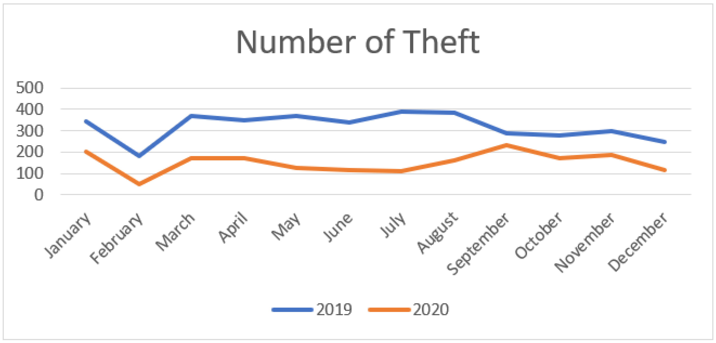
As is shown in Figure 1, in terms of monthly numbers, February had the lowest number of thefts, with 181 thefts in February 2019 (pre-COVID-19) and 52 crimes in February 2020 (during COVID-19). In all other months in 2019, >240 thefts were committed per month, and >110 thefts were committed per month in all other months in 2020.

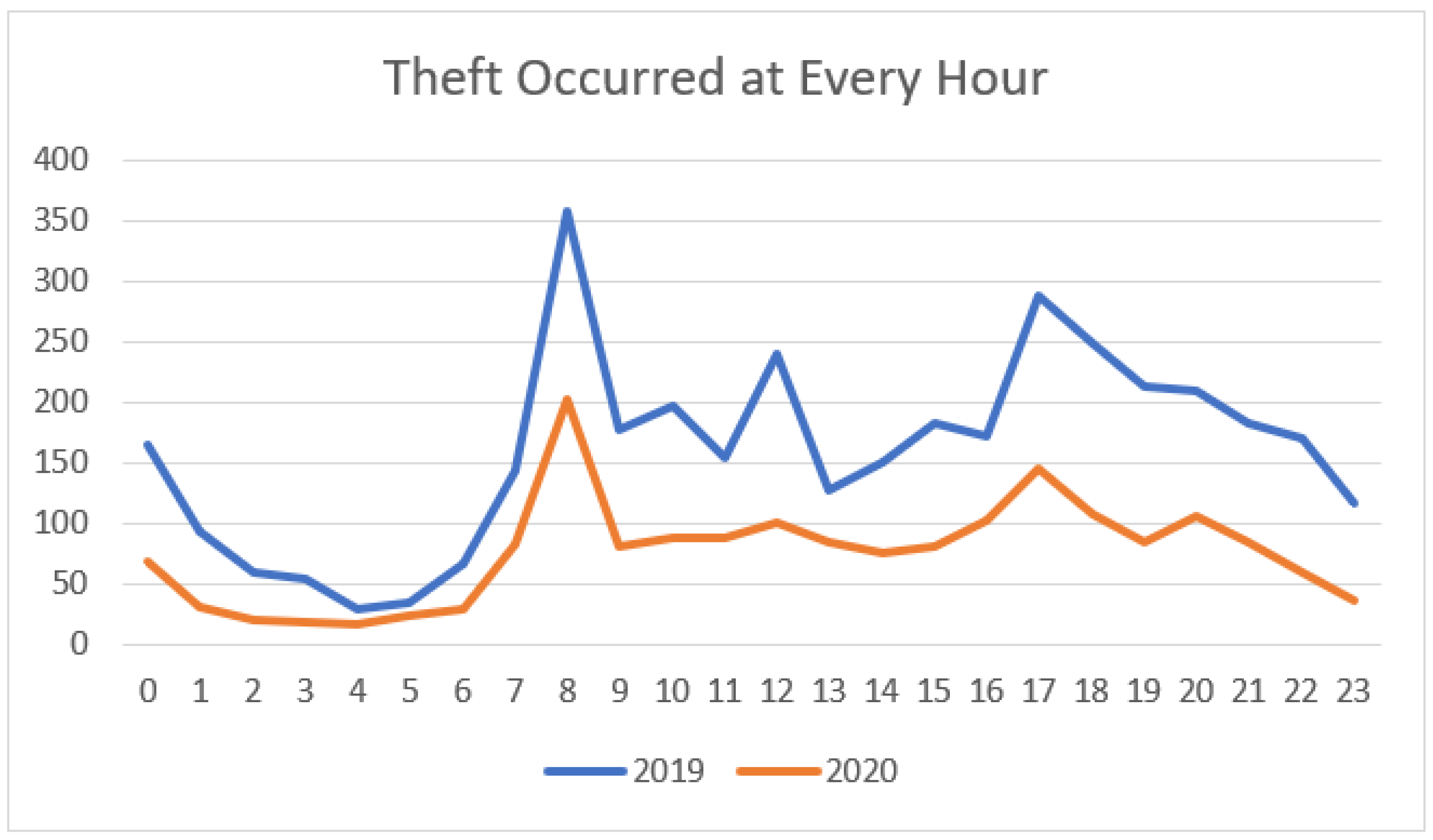
As is shown in Figure 2, regarding the time of day, 8:00–9:00 and 17:00–18:00 were the peak commuting periods, during which more theft occurred both in 2019 (pre-COVID-19) and 2020 (during COVID-19).

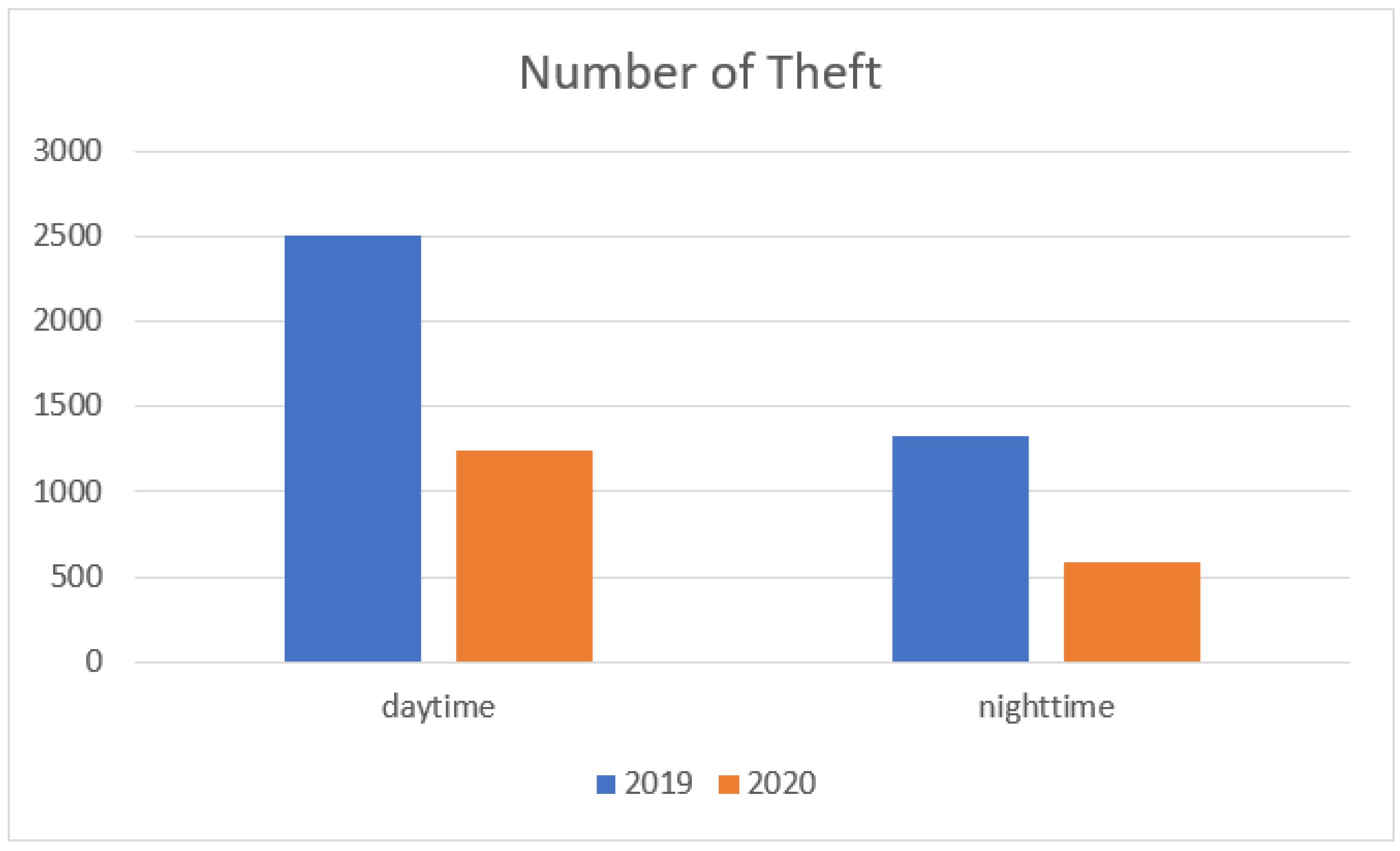
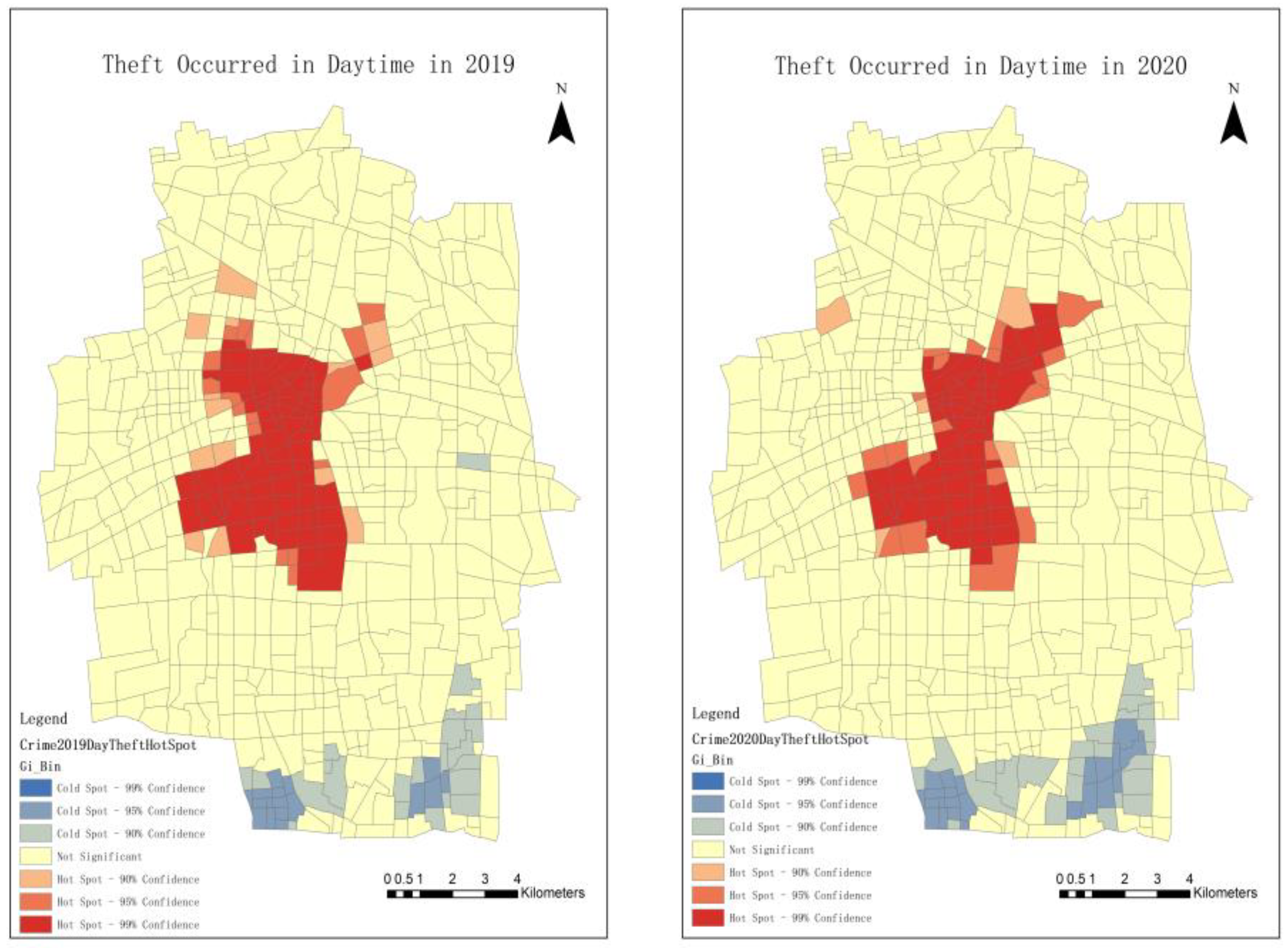
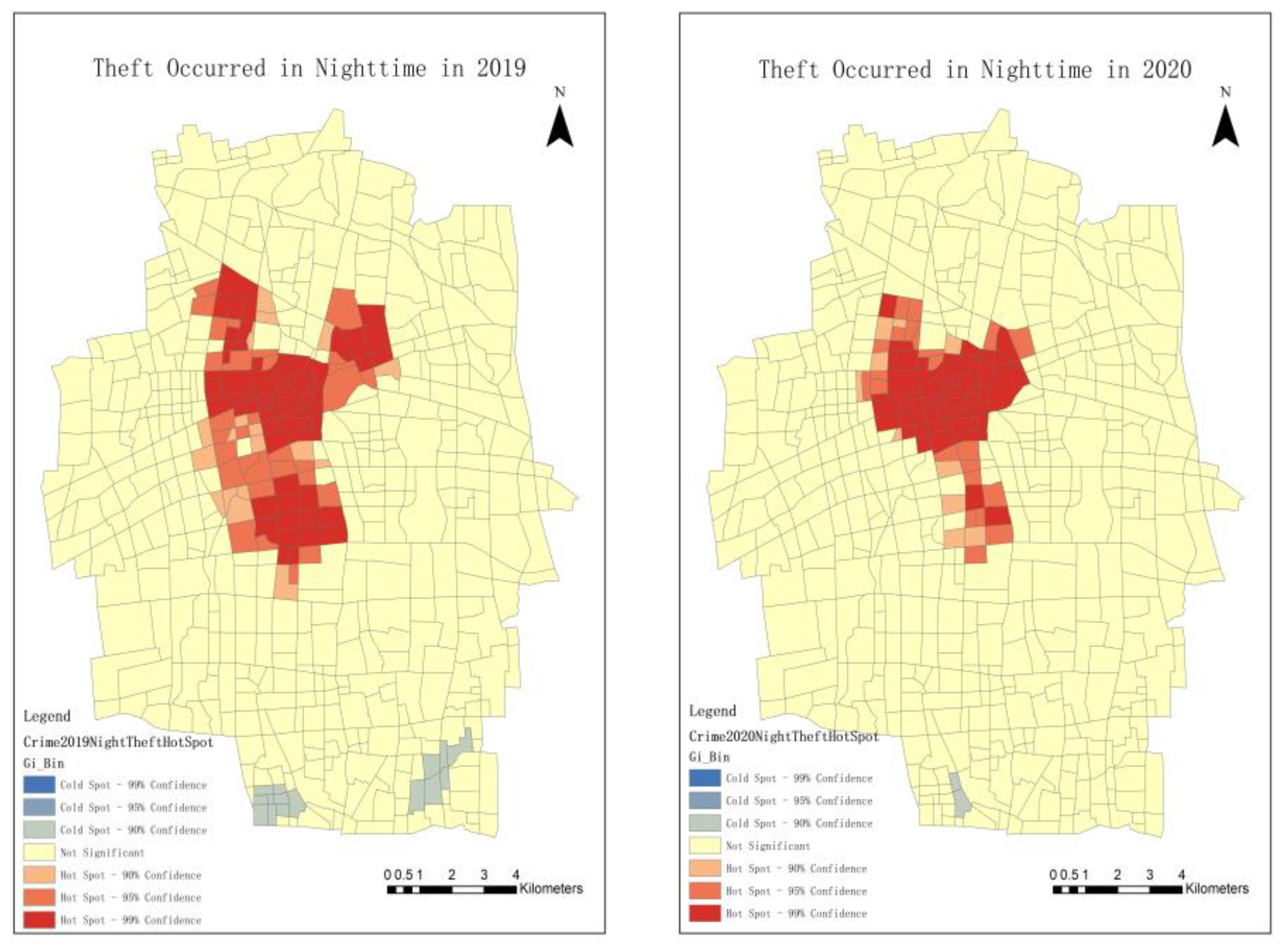
We counted the number of thefts that occurred after 8:00 and before 20:00 as daytime thefts and those that occurred after 20:00 and before 8:00 the next day as nighttime thefts. As is shown in Figure 3, when comparing daytime and nighttime hours, more theft occurred during the day than at night.

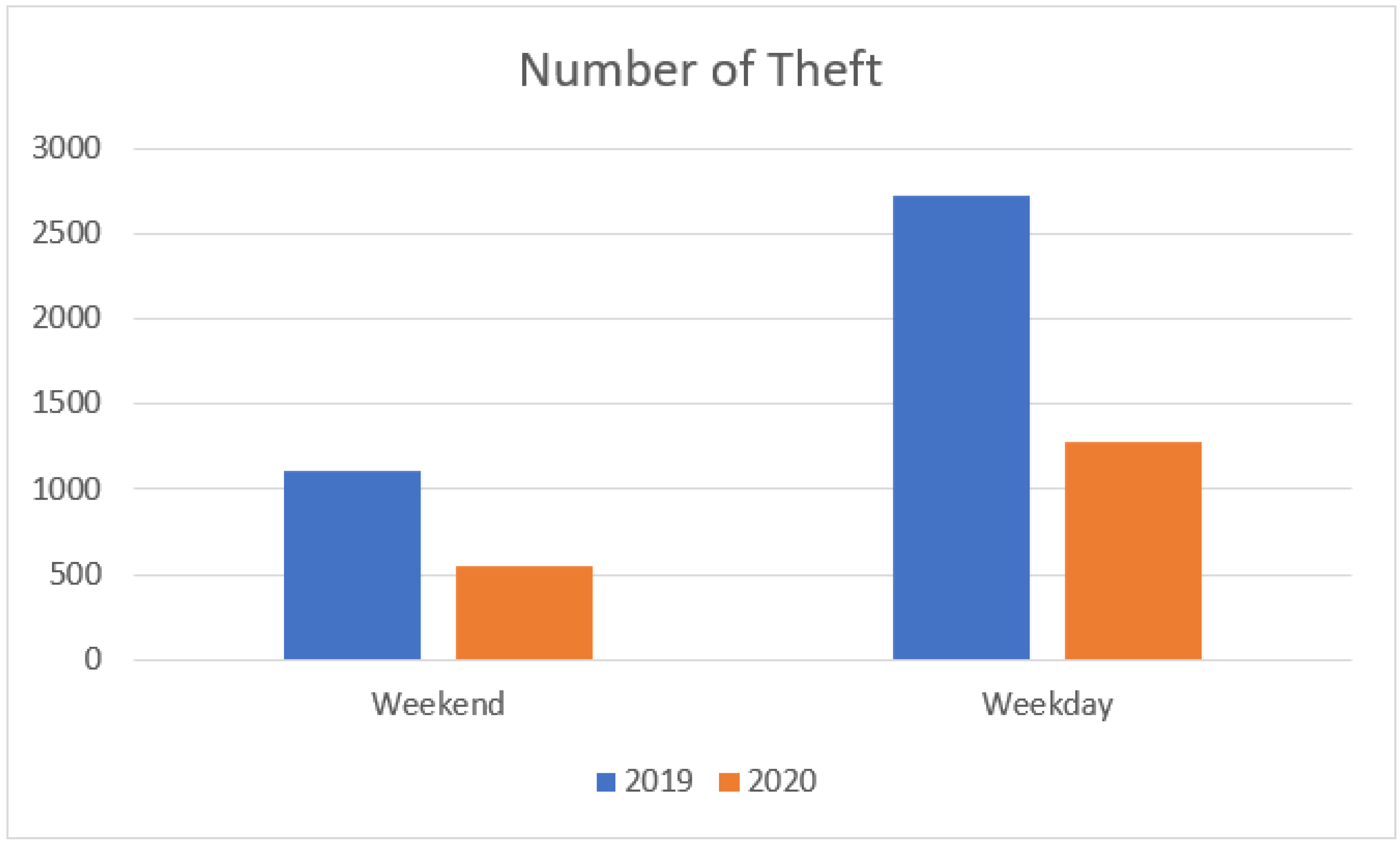
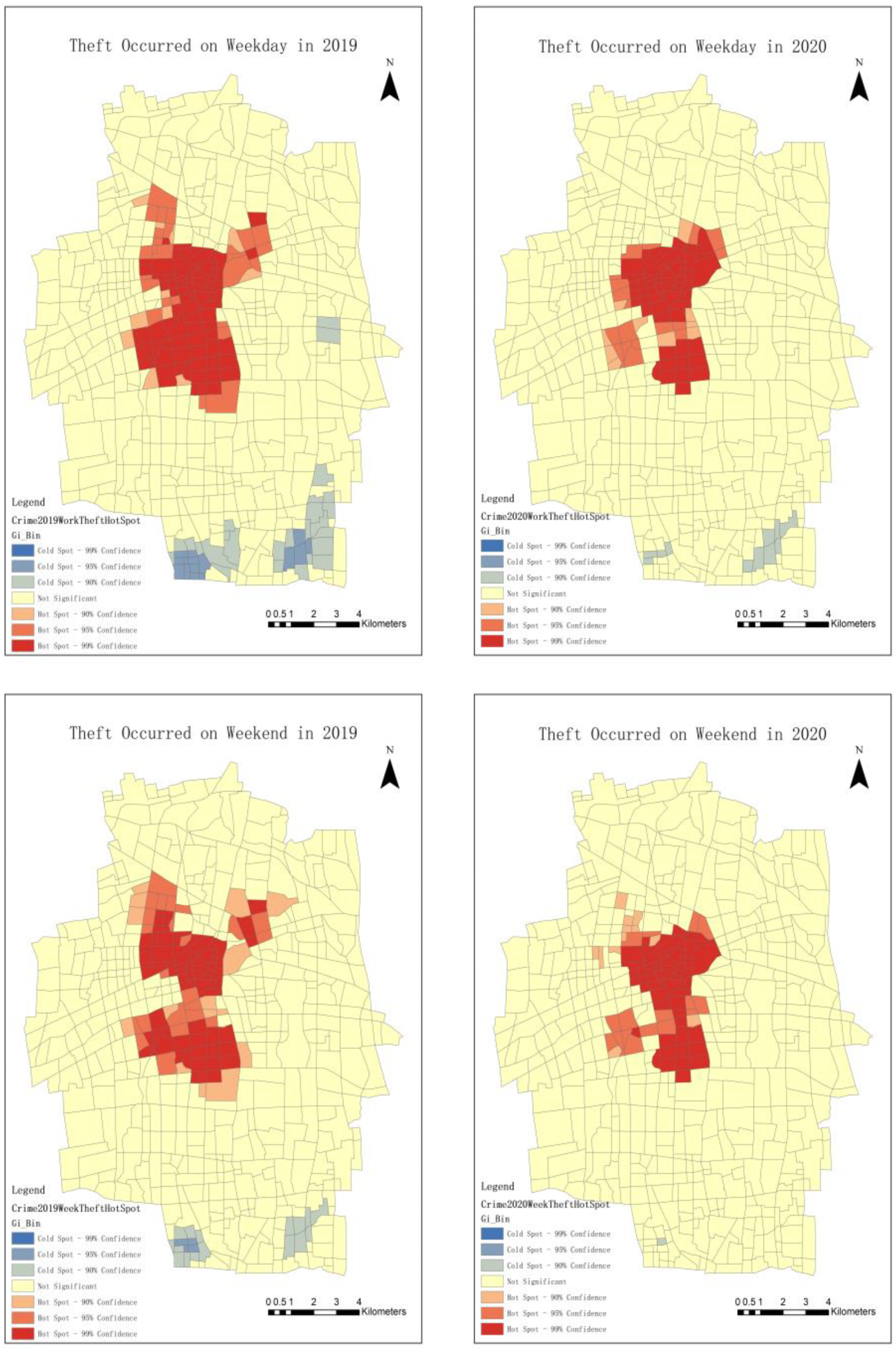
The number of thefts on weekdays and weekends was calculated based on the occurrence dates of thefts in 2019 and 2020. As is shown in Figure 4, it was found that the number of thefts on weekdays pre- and during-COVID-19 was higher than that on weekends.

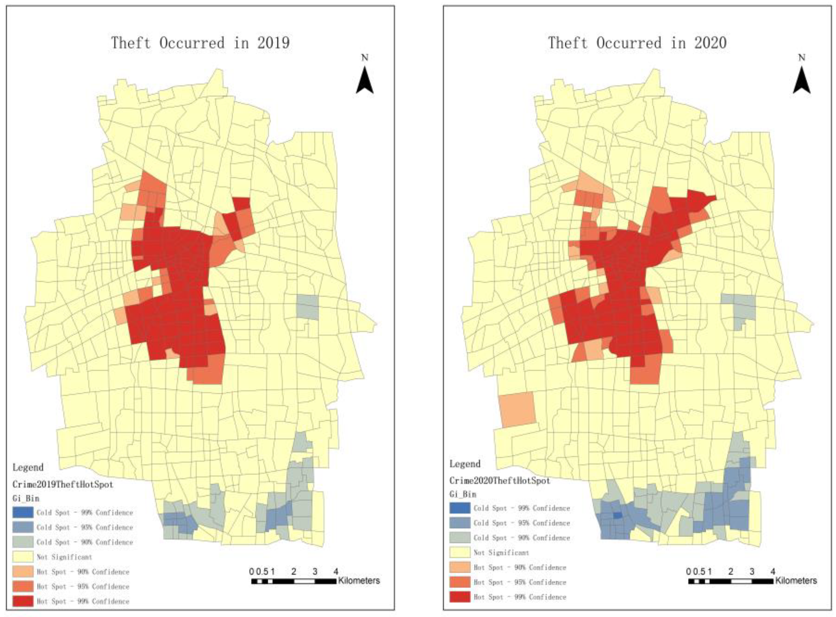
4.2. Spatial Distribution Characteristics of Theft

By analyzing the spatial distribution of thefts in the pre- and during-COVID-19 periods, we found that the hot spots of theft were concentrated in the central region of the study area, with slightly different boundaries between the two years. The cold spot areas were located mainly in the southern part of the study area, and the cold spot area increased during the COVID-19 period. The hot spot characteristics of theft distribution at the neighborhood scale are shown in Figure 5.

The hotspot range of theft shifted to the northeast during the day in the COVID-19 period, and the cold spot area was increased; the hotspot area decreased more significantly at night. The hotspot characteristics of theft distribution during one day are shown in Figure 6.

In both the pre- and COVID-19 periods, hotspots were concentrated in the central area, and hotspots decreased on both weekdays and weekends during the COVID-19 period. The characteristics of theft distribution are shown in Figure 7.

4.3. Spatial Autocorrelation Characteristics of Impact Factors

We analyzed the Moran’s I calculation results to discern the spatial distribution patterns of the dataset. The minimum value of Moran’s I is −1, and the maximum value is 1. When Moran’s I is < 0, the attribute values of the dataset have a discrete distribution pattern in space. When Moran’s I is closer to −1, similar values have obvious dispersions in space, and very different values have obvious clustering in space (“high–low” clustering or “low–high” clustering). If Moran’s I is > 0, the attribute values of the dataset show a spatial aggregation distribution pattern. When Moran’s I is closer to 1, similar values have an obvious spatial aggregation (“high–high” aggregation or “low–low” aggregation). If Moran’s I is 0, the attribute values of the dataset are randomly distributed in space and there is no spatial autocorrelation.

The results of the Moran’s I test in the pre- and COVID-19 periods are shown in

Table 1. Moran’s I index test results pre-COVID-19.

	Moran’s I Index	Expected Index	Variance	z-Score	p-Value
X1	0.942931	−0.001786	0.000412	46.514893	0.000000
X2	0.610315	−0.001786	0.000413	30.107576	0.000000
X3	0.922103	−0.001786	0.000413	45.458592	0.000000
X4	1.025135	−0.001786	0.000411	50.681494	0.000000
X5	0.802339	−0.001786	0.000409	39.750823	0.000000
X6	1.000710	−0.001786	0.000406	49.773963	0.000000
X7	0.855719	−0.001786	0.000411	42.296918	0.000000
X8	0.235030	−0.001786	0.000379	12.167346	0.000000
X9	0.494608	−0.001786	0.000411	24.499080	0.000000
X10	0.724707	−0.001786	0.000413	35.760625	0.000000
X11	1.059239	−0.001786	0.000413	52.215374	0.000000
X12	1.079792	−0.001786	0.000411	53.372033	0.000000
X13	0.995083	−0.001786	0.000413	49.048678	0.000000
X14	0.504677	−0.001786	0.000413	24.934092	0.000000

and

Table 2. Moran’s I index test results during the COVID-19 period.

	Moran’s I Index	Expected Index	Variance	z-Score	p-Value
X1	0.852175	−0.001786	0.000413	42.043374	0.000000
X2	0.538961	−0.001786	0.000413	26.596872	0.000000
X3	0.832803	−0.001786	0.000413	41.054320	0.000000
X4	0.768857	−0.001786	0.000411	38.011347	0.000000
X5	0.538303	−0.001786	0.000409	26.718267	0.000000
X6	0.649939	−0.001786	0.000407	32.307992	0.000000
X7	0.913006	−0.001786	0.000412	45.078005	0.000000
X8	0.335604	−0.001786	0.000399	16.898551	0.000000
X9	0.400080	−0.001786	0.000410	19.847979	0.000000
X10	0.722516	−0.001786	0.000413	35.638922	0.000000
X11	0.943492	−0.001786	0.000413	46.514503	0.000000
X12	0.985522	−0.001786	0.000411	48.696948	0.000000
X13	1.005885	−0.001786	0.000413	49.572372	0.000000
X14	0.504381	−0.001786	0.000413	24.919512	0.000000

. We found that all Moran’s I values for 14 independent variables were >0, and the corresponding p-statistic values of all independent variables were <0.05 (the significance level was set at 0.05). Thus, the null hypothesis (the alternative independent variables did not have spatial autocorrelation) was rejected, and the results indicated that all of the alternative independent variables selected in this study had some spatial autocorrelation. At the same time, all the independent variables had positive z-score values and were >2.58, which further indicated that the alternative independent variables had strong spatial aggregation characteristics and met the conditions for constructing the GWR model in both the pre- and COVID-19 periods.

4.4. Geographically Weighted Regression Analysis

The dependent variable of this study was the number of thefts in each neighborhood in 2019 and 2020. According to criminological theory, crime is related to many factors [34]. The point of interest data of this study is closely related to the RAT [42]. The independent variables were mainly taken from the POI data, including X1–X13, and X14 was the demographic data. The variables can be divided into the three categories of functional facilities, transportation conditions, and socioeconomic conditions. The list of influencing factors (independent variables) is shown in

Table 3. List of influencing factors (independent variables).

Classification	Variable Name	Description	Variable Number
Functional Facilities	Dining and Gourmet	Number of dining and gourmet establishments per unit area in the neighborhood	X1
	Company and Enterprise	Number of companies and enterprises per unit area in the neighborhood	X2
	Shopping and Consumption	Number of supermarkets, convenience stores, and stores per unit area in the neighborhood	X3
	Sports and Leisure Services	Number of outdoor fitness places, fitness centers, campgrounds, golf courses, taekwondo facilities, ice and snow sports facilities, billiards facilities, swimming facilities, soccer facilities, table tennis facilities, badminton facilities, pensioner vacation facilities, chess and card rooms, KTV bars, farmhouses, Internet cafes, bars, and playgrounds per unit area in the neighborhood	X4
	Financial Institutions	Number of banks, ATMs, insurance offices, and investment banking offices per unit area in the neighborhood	X5
	Hotel Accommodation	Number of hotels, star hotels, and hotel chains per unit area in the neighborhood	X6
	Science, Education, and Culture	Number of kindergartens, primary and secondary schools, research units, training units, conventions, and higher education institutions per unit area in the neighborhood	X7
	Tourist Attractions	Number of parks, squares, monuments, and religious institutions per unit area in the neighborhood	X8
	Automotive Related	Number of gas stations, charging stations, car repair shops, car maintenance shops, and car dealers per unit area in the neighborhood	X9
	Business and Residence	Number of residential areas, dormitories, industrial parks, office buildings, commercial and residential buildings, and community centers per unit area in the neighborhood	X10
	Life Services	Number of intermediaries, beauty salons, telecommunication business halls, public toilets, logistics, bathing and massage sites, launderettes, and lottery sale locations per unit area in the neighborhood	X11
	Healthcare	Number of general hospitals, specialty hospitals, emergency centers, pharmacies, animal medical care clinics, and clinics per unit area in the neighborhood	X12
Transportation Conditions	Transportation Facilities	Number of subways, bus stops, parking lots, toll booths, port terminals, and trains per unit area in the neighborhood	X13
Socioeconomic	Resident Population Density	Resident population per unit area in the neighborhood	X14

.

The values of the independent variables varied widely and did not satisfy a normal distribution, and thus we obtained the final values of the independent variables using Log transformation. Before using the GWR model, we checked the multicollinearity of the two datasets. For the dataset before COVID-19, all variance inflation factor (VIF) values were <10. Additionally, most were <5, except for X3 and X11. For the dataset during COVID-19, all VIF values were <10. Additionally, most were <5, except for X3, X11, and X13. Therefore, the two datasets could be used in the GWR model.

Before using the GWR model for the case analysis, we had to find the appropriate weight function and bandwidth. In this study, through a large number of simulations, comparisons, and analyses, we selected the adjusted exponential spatial weight function and the cross-validation (CV) method to optimize the bandwidth selection.

From

Table 4. Pre-COVID-19 parameter values calculated by different models.

	Global Regression	GWR
AIC	612.68356	334.823043
AICc	613.564294	532.640665
Residual sum of squares	92.474266	47.851422
R2	0.669023	0.828734
Adjusted R2	0.659914	0.744762

and

Table 5. Parameter values during the COVID-19 period calculated by different models.

	Global Regression	GWR
AIC	724.96088	479.972983
AICc	725.841614	675.206209
Residual sum of squares	112.963892	62.105284
R2	0.475052	0.711394
Adjusted R2	0.460604	0.57002

, we can see that both the R² and adjusted R² values were larger than the corresponding values of the ordinary linear regression. This result indicates that the simulation of the GWR model was better than the ordinary linear regression model.

In Table 4 and Table 5, the adjusted R² is a multiple determination coefficient obtained by adjusting R². This value can be used to measure the regression fit of the regression model, and the higher its value, the better it explains the relationship between the dependent variable and the independent variable. As Table 4 shows, the R² and adjusted R² values of the dependent variable increased compared with the global regression, with the R² value increasing by 0.159711 and the adjusted R² value increasing by 0.084848. In Table 5, it can be seen that the R² value increased by 0.236342 and the adjusted R² value increased by 0.109416. This result indicates that GWR was a better fit for the relationship between theft and influencing factors and has more explanatory power compared with ordinary linear regression that was used throughout the study. In addition, we found that both the Akaike information criterion (AIC) and AICc values of GWR converged compared with the ordinary linear regression, which indicated that GWR was more sensitive to the datasets and significantly improved the fitting performance. In conclusion, the GWR model had more explanatory power for the independent variable influences on the dependent variable (theft) and exhibited a significant improvement compared to the ordinary linear regression method.

We used POI datasets for the GWR analysis. The spatial distribution of regression coefficients for all case impact factors in the study area of the GWR model are shown in Figure S1 for the pre- and COVID-19 periods. The summary of GWR coefficient estimates in the pre- and COVID-19 periods are shown in

Table 6. Summary of GWR coefficient estimates pre-COVID-19.

Name	Min	1st Qu	Median	3rd Qu	Max
Intercept	−0.102	0.242	0.409	0.638	1.030
X1	−0.188	0.056	0.109	0.200	0.361
X2	−0.152	−0.031	0.003	0.039	0.255
X3	−0.074	0.095	0.157	0.216	0.405
X4	−0.163	0.041	0.105	0.136	0.288
X5	−0.151	−0.067	−0.033	−0.002	0.084
X6	−0.191	−0.098	−0.062	0.002	0.115
X7	−0.206	−0.087	0.000	0.082	0.397
X8	0.013	0.104	0.161	0.201	0.684
X9	−0.174	−0.070	−0.028	0.005	0.093
X10	−0.086	0.047	0.125	0.327	0.597
X11	−0.129	0.069	0.135	0.194	0.493
X12	−0.103	−0.014	0.034	0.093	0.304
X13	−0.159	−0.016	0.078	0.137	0.277
X14	−0.104	0.008	0.037	0.062	0.163

Min, minimum; 1st Qu, the first quarter; 3rd Qu, the third quarter; Max, maximum.

and

Table 7. Summary of GWR coefficient estimates during the COVID-19 period.

Name	Min	1st Qu	Median	3rd Qu	Max
Intercept	−0.391	0.023	0.158	0.315	0.645
X1	−0.367	−0.065	0.029	0.076	0.175
X2	−0.113	−0.025	0.016	0.046	0.121
X3	−0.371	−0.037	0.018	0.061	0.204
X4	−0.268	−0.093	−0.042	0.007	0.175
X5	−0.213	−0.153	−0.099	−0.037	0.107
X6	−0.170	−0.086	0.069	0.210	0.445
X7	−0.206	0.002	0.09	0.177	0.286
X8	−0.041	0.216	0.324	0.420	0.791
X9	−0.128	−0.035	0.021	0.132	0.280
X10	−0.146	−0.036	0.039	0.128	0.454
X11	−0.146	−0.007	0.037	0.093	0.292
X12	−0.285	−0.028	0.068	0.178	0.384
X13	−0.094	0.172	0.255	0.327	0.559
X14	0.010	0.080	0.117	0.158	0.226

Min, minimum; 1st Qu, the first quarter; 3rd Qu, the third quarter; Max, maximum.

.

The effects of tourist attractions (X8) were positively correlated, and there was little difference between the pre- and COVID-19 periods.

The effects of dining and gourmet (X1), shopping and consumption (X3), business and residence (X10), and life services (X11) were overwhelmingly positively correlated in the pre-COVID-19 period. The basic life and work-related areas such as restaurants and food, shopping, living services, and business residences were all hot spots for theft, but due to the impact of COVID-19, thefts were negatively correlated with the above factors during COVID-19, which may be due to the COVID-19 prevention and control policies and the reduced frequency of residents going outside.

Transportation facilities (X13) and resident population density (X14) were most positively correlated with thefts during COVID-19, which indicated that these two factors are key targets for the prevention and control of theft in the COVID-19 period and that densely populated areas, transportation facilities, and distribution areas require strengthened security and control.

The effect of sports and leisure service facilities (X4) was mostly positively correlated pre- COVID-19 and was mostly negatively correlated in the during COVID-19. The effect of hotel accommodations (X6) was negatively correlated pre-COVID-19 and was negatively correlated in the northern region but positively correlated in both the south and west during the COVID-19 period. This is likely because the population flow was less intense during the COVID-19 period, especially in the northern region, while the population flow was greater in the pre-COVID-19 period, and the suppression of the surrounding population was obvious. Hotel accommodations (X6) were the public security focus of the deployment of video surveillance, and its deterrent effect on theft was great.

The effect of companies and enterprises (X2) had similar impacts in the pre- and COVID-19 periods, indicating that COVID-19 had little impact on theft around companies and enterprises. The effect of financial institutions (X5) was positively correlated with theft in the COVID-19 period and shifted to the west. The effect of science, education, and culture facilities (X7) was different in the north and south, with a positive correlation being seen in the south and a negative correlation observed in the north pre-COVID-19; negative correlations were identified in the west and northwest during the COVID-19 period. The positive correlation effect of automotive-related facilities (X9) shifted to the northern region during the COVID-19 period. The negative correlation effect of healthcare facilities (X12) was located in the center and the eastern region, and negative correlations appeared in the northern region during the COVID-19 period.

A detailed analysis of the results of the GWR model demonstrated its ability to discriminate the spatial heterogeneity of the factors influencing theft. Different influencing factors had different theft coefficients; thus, crime prevention and control can be carried out through the analysis of different regional influencing factors. The spatiotemporal characteristics, spatial distribution, and influencing factors of theft in the pre- and COVID-19 periods were different. The study of quantitative relationships has strong significance for guiding security prevention and control. Prevention and control efforts should be strengthened for those influencing factors that were positively correlated, especially those with larger coefficients, to prevent the occurrence of theft.

5. Conclusions and Discussion

In this study, we conducted a spatiotemporal analysis and geographic modeling using spatiotemporal big data, demographic data, neighborhood data, and theft data. This study analyzed the theft data of Haining City in the pre- and COVID-19 periods using mathematical statistical methods. The number of thefts decreased significantly in the COVID-19 period. The daily, weekly, and monthly trends were similar in the pre- and COVID-19 periods. The hotspot spatial distribution area decreased in the during COVID-19. A greater number of thefts occurred during the peak commuting periods, and a greater number occurred during the day than at night. In terms of police deployment and public security prevention and control, it is necessary to increase police patrols in the peak months and hours of theft so as to have a deterrent effect on theft.

When using the hot spot analysis (Getis-Ord Gi*) method to analyze the theft hot spots in 2019 and 2020, the results showed that the theft hot spots were clustered, with 99% confidence level hot spot areas being concentrated in the center of the study area and 90% confidence level cold spot areas being concentrated in the south of the study area. In the hot spot area, police patrol, video surveillance deployment, and other measures should be increased. In the cold spot area, these measures should be appropriately reduced. For the global spatial autocorrelation analysis, we used Moran’s I index to test the results in the pre- and COVID-19 periods. All the Moran’s I indexes were >0, and all the z-score values were >2.58, with obvious clustering benefits. These results can help guide precise police deployment to theft hot spots. Mathematical analysis and temporal distribution characteristics can support urban planning and enhance public safety. In hot spot areas, police prevention and control measures need to be increased by implementing measures such as video surveillance, patrol cars, and security booths, and police presence can be reduced in cold spot areas.

We used the GWR model to detect the spatial variation pattern of the local regional regression coefficients of theft in Haining City and to explain the relationship between theft and their influencing factors. After analyzing the model regression results, we found that thefts in the study area were not smoothly distributed in space. Through an analysis of the GWR model results, we found that the effect of tourist attractions was positively correlated with theft, with little difference between the pre- and COVID-19 periods. The effects of dining and gourmet, shopping and consumption, business and residence, and life service areas varied greatly. These four factors are related to basic life and work and represent densely populated areas for theft, but due to the impact of COVID-19, theft was negatively correlated with the above factors during the pandemic, which may be related to the COVID-19 prevention and control policies implemented in this city. The other influencing factors were different in terms of their spatial distribution. Police prevention and control measures can be adjusted according to the influencing factors of theft in the pre- and COVID-19 periods. Points of interest that strongly positively correlate with theft require an increased police presence, and vice versa. In urban public security planning, land use planning should be conducted to reduce the agglomeration of factors with a great influence on the crime rate. Combined with police planning, video surveillance should be deployed to reduce the occurrence of theft, increase the efficiency of theft detection, and ensure the safety of the public’s lives and property. The results of this study are important for understanding the spatial evolution of crime under the influence of major public health emergencies and for formulating scientific strategies for crime prevention and control.

Crime is a complex phenomenon that is the result of a combination of multiple factors. More studies on influence factors and internal relationships should be added to explore the influence mechanism of theft and other types of crime under different scenarios. By looking at different types of crime and time points of crime occurrence, we can study the impact of crime more granularly in order to tackle it with better placed video surveillance in the future. For example, according to the time smoothness of daily changes over the course of a week, we can focus on the regular characteristics and mechanisms of action under daily changes. For different types of crime, we can analyze the R² value and adjusted R² and AIC values using the GWR model, which can be used to study the mechanism of action of crime impact. Additionally, we will distinguish the types of theft and conduct more refined studies from different perspectives in future work. Based on the POI data from multiple years, the length of the research time series should be increased to study the impact characteristics of crime in different years. Video surveillance deployment should be closely integrated with factors of high crime impact to have a greater inhibitory effect on crime. However, the deployment of video surveillance does not necessarily and inevitably reduce the occurrence of crime, because the crime rate is related to the type of crime, the time of the crime, and other influencing factors of crime.

References

1. Zhu, X. A Preliminary Exploration of Crime Geography. J. Hebei Norm. Univ. Philos. Soc. Sci. Edit. 1986, 3, 113–118. [Google Scholar]
2. Guerry, A.-M. Essai Sur La Statistique Morale De La France; Kessinger Publishing: Paris, France, 1833. [Google Scholar]
3. Ceccato, V.; Haining, R.; Kahn, T. The geography of homicide in São Paulo, Brazil. Environ. Plan. A 2007, 39, 1632–1653. [Google Scholar] [CrossRef]
4. Shaw, C.R.; McKay, H.D. Juvenile Delinquency and Urban Areas; University of Chicago Press: Chicago, IL, USA, 1942. [Google Scholar]
5. Browning, C.R.; Byron, R.A.; Calder, C.A.; Krivo, L.J.; Kwan, M.-P.; Lee, J.-Y.; Peterson, R.D. Commercial density, residential concentration, and crime: Land use patterns and violence in neighborhood context. J. Res. Crime Delinq. 2010, 47, 329–357. [Google Scholar] [CrossRef]
6. Wolfe, M.K.; Mennis, J. Does vegetation encourage or suppress urban crime? Evidence from Philadelphia, PA. Landsc. Urban Plan. 2012, 108, 112–122. [Google Scholar] [CrossRef]
7. Bernasco, W. Modeling micro-level crime location choice: Application of the discrete choice framework to crime at places. J. Quant. Criminol. 2010, 26, 113–138. [Google Scholar] [CrossRef]
8. Schweitzer, J.H.; Kim, J.W.; Mackin, J.R. The impact of the built environment on crime and fear of crime in urban neighborhoods. J. Urban Technol. 1999, 6, 59–73. [Google Scholar] [CrossRef]
9. Boessen, A.; Hipp, J.R. Close-ups and the scale of ecology: Land uses and the geography of social context and crime. Criminology 2015, 53, 399–426. [Google Scholar] [CrossRef]
10. Mao, Y.; Dai, S. Reasearch on Spatial and Enviornmental Characters of Crimes: Case Study of Shanghai. J. Urban Plan. 2006, 3, 85–93. [Google Scholar]
11. Zhou, S.; Xie, W.; Song, G.; Liu, L. The Spatial Differentiation Effect of Land Use on Street Robbery: A Case Study in H City, China. Sci. Geogr. Sin. 2017, 37, 885–894. [Google Scholar]
12. Zhang, X.; Chen, P. The Impact of Urban Facilities on Crime during the Pre-and Pandemic Periods: A Practical Study in Beijing. Int. J. Environ. Res. Public Health 2023, 20, 2163. [Google Scholar] [CrossRef]
13. Yang, M.; Chen, Z.; Zhou, M.; Liang, X.; Bai, Z. The impact of COVID-19 on crime: A spatial temporal analysis in Chicago. ISPRS Int. J. Geo-Inf. 2021, 10, 152. [Google Scholar] [CrossRef]
14. Campedelli, G.M.; Favarin, S.; Aziani, A.; Piquero, A.R. Disentangling community-level changes in crime trends during the COVID-19 pandemic in Chicago. Crime Sci. 2020, 9, 21. [Google Scholar] [CrossRef] [PubMed]
15. Halford, E.; Dixon, A.; Farrell, G.; Malleson, N.; Tilley, N. Crime and coronavirus: Social distancing, lockdown, and the mobility elasticity of crime. Crime Sci. 2020, 9, 11. [Google Scholar] [CrossRef] [PubMed]
16. Nivette, A.E.; Zahnow, R.; Aguilar, R.; Ahven, A.; Amram, S.; Ariel, B.; Burbano, M.J.A.; Astolfi, R.; Baier, D.; Bark, H.-M. A global analysis of the impact of COVID-19 stay-at-home restrictions on crime. Nat. Hum. Behav. 2021, 5, 868–877. [Google Scholar] [CrossRef]
17. Ashby, M.P. Initial evidence on the relationship between the coronavirus pandemic and crime in the United States. Crime Sci. 2020, 9, 6. [Google Scholar] [CrossRef] [PubMed]
18. Ceccato, V.; Kahn, T.; Herrmann, C.; Östlund, A. Pandemic restrictions and spatiotemporal crime patterns in New York, São Paulo, and Stockholm. J. Contemp. Crim. Justice 2022, 38, 120–149. [Google Scholar] [CrossRef]
19. Sun, Y.; Huang, Y.; Yuan, K.; Chan, T.O.; Wang, Y. Spatial patterns of COVID-19 incidence in relation to crime rate across London. ISPRS Int. J. Geo-Inf. 2021, 10, 53. [Google Scholar] [CrossRef]
20. Carter, T.M.; Turner, N.D. Examining the immediate effects of COVID-19 on residential and commercial burglaries in Michigan: An interrupted time-series analysis. J. Crim. Justice 2021, 76, 101834. [Google Scholar] [CrossRef]
21. Langton, S.; Dixon, A.; Farrell, G. Small area variation in crime effects of COVID-19 policies in England and Wales. J. Crim. Justice 2021, 75, 101830. [Google Scholar] [CrossRef]
22. Mohler, G.; Bertozzi, A.L.; Carter, J.; Short, M.B.; Sledge, D.; Tita, G.E.; Uchida, C.D.; Brantingham, P.J. Impact of social distancing during COVID-19 pandemic on crime in Los Angeles and Indianapolis. J. Crim. Justice 2020, 68, 101692. [Google Scholar] [CrossRef]
23. Andresen, M.A.; Hodgkinson, T. Somehow I always end up alone: COVID-19, social isolation and crime in Queensland, Australia. Crime Sci. 2020, 9, 1–20. [Google Scholar] [CrossRef] [PubMed]
24. Schleimer, J.P.; Pear, V.A.; McCort, C.D.; Shev, A.B.; De Biasi, A.; Tomsich, E.; Buggs, S.; Laqueur, H.S.; Wintemute, G.J. Unemployment and crime in US cities during the coronavirus pandemic. J. Urban Health 2022, 99, 82–91. [Google Scholar] [CrossRef] [PubMed]
25. Kaukinen, C. When stay-at-home orders leave victims unsafe at home: Exploring the risk and consequences of intimate partner violence during the COVID-19 pandemic. Am. J. Crim. Justice 2020, 45, 668–679. [Google Scholar] [CrossRef] [PubMed]
26. Almulhim, T.S.; Barahona, I. Decision support system for ranking relevant indicators for reopening strategies following COVID-19 lockdowns. Qual. Quant. 2022, 56, 463–491. [Google Scholar] [CrossRef] [PubMed]
27. Chen, T.; Bowers, K.; Zhu, D.; Gao, X.; Cheng, T. Spatio-temporal stratified associations between urban human activities and crime patterns: A case study in San Francisco around the COVID-19 stay-at-home mandate. Comput. Urban Sci. 2022, 2, 13. [Google Scholar] [CrossRef] [PubMed]
28. McCarthy, M.; Homel, J.; Ogilvie, J.; Allard, T. Initial impacts of COVID-19 on youth offending: An exploration of differences across communities. J. Criminol. 2021, 54, 323–343. [Google Scholar] [CrossRef]
29. Weisburd, D.; Mazerolle, L.G. Crime and disorder in drug hot spots: Implications for theory and practice in policing. Police Q. 2000, 3, 331–349. [Google Scholar] [CrossRef]
30. Sherman, L.W.; Gartin, P.R.; Buerger, M.E. Hot spots of predatory crime: Routine activities and the criminology of place. Criminology 1989, 27, 27–56. [Google Scholar] [CrossRef]
31. Ratcliffe, J.H. Crime mapping and the training needs of law enforcement. Eur. J. Crim. Policy Res. 2004, 10, 65–83. [Google Scholar] [CrossRef]
32. Mahmood, S. Exploring COVID-19 incidence hotspot in Metropolitan area of Pakistan using geo-statistical approach: A study of Lahore city. Spat. Inf. Res. 2022, 30, 469–476. [Google Scholar] [CrossRef]
33. Henrico, I.; Mayoyo, N.; Mtshawu, B. Understanding crime in the context of COVID-19. S. Afr. Crime Q. 2022, 71, 2413–3108. [Google Scholar]
34. Maiti, A.; Zhang, Q.; Sannigrahi, S.; Pramanik, S.; Chakraborti, S.; Cerda, A.; Pilla, F. Exploring spatiotemporal effects of the driving factors on COVID-19 incidences in the contiguous United States. Sustain. Cities Soc. 2021, 68, 102784. [Google Scholar] [CrossRef] [PubMed]
35. Liu, L.; Du, F.; Xiao, L.; Song, G.; Liu, K.; Jiang, C. The density of various road types and larceny rate:An empiricalanalysis of zg city. Hum. Geogr. 2017, 32, 32–38. [Google Scholar]
36. Yan, J.; Shu, X.; Yuan, H. Relationship between spatial distribution of thief crime and geographical factors. J. Tsinghua Uni. 2010, 50, 197–202. [Google Scholar]
37. Fotheringham, A.S.; Brunsdon, C.; Charlton, M. Geographically Weighted Regression: The Analysis of Spatially Varying Relationships; John Wiley & Sons: Hoboken, NJ, USA, 2003. [Google Scholar]
38. Fotheringham, A.S.; Charlton, M.E.; Brunsdon, C. Geographically weighted regression: A natural evolution of the expansion method for spatial data analysis. Environ. Plan. A 1998, 30, 1905–1927. [Google Scholar] [CrossRef]
39. Brunsdon, C.; Fotheringham, A.S.; Charlton, M.E. Geographically weighted regression: A method for exploring spatial nonstationarity. Geogr. Anal. 1996, 28, 281–298. [Google Scholar] [CrossRef]
40. Wang, Z. Temporal-Spatial Hot Spot Analysis on Crime Cases Based on ScanStatistics Methodologies in Shanghai; East China Normal University: Shanghai, China, 2013. [Google Scholar]
41. Bao, S.; Wang, Z. Research and Practice of Crime SpatialTemporal Scan Statistics Methodology. Microcomput. Appl. 2017, 33, 63–66. [Google Scholar]
42. Cohen, L.E.; Felson, M. Social change and crime rate trends: A routine activity approach (1979). In Classics in Environmental Criminology; Routledge: New York, NY, USA, 2010; pp. 203–232. [Google Scholar]
43. Patricia, B.; Paul, B. Criminality of place: Crime generators and crime attractors. Eur. J. Crim. Policy Res. 1995, 3, 5–26. [Google Scholar]
44. Clarke, R.V.G.; Felson, M. Routine Activity and Rational Choice; Transaction publishers: Piscataway, NJ, USA, 1993; Volume 5. [Google Scholar]
45. Webb, B.; Laycock, G. Tackling Car Crime: The Nature and Extent of the Problem; Home Office, Crime Prevention Unit: London, UK, 1992. [Google Scholar]
46. Matthews, R. Developing more effective strategies for curbing prostitution. Secur. J. 1990, 1, 182–187. [Google Scholar]
47. Jeffery, C.R. Crime Prevention through Environmental Design; Sage: Beverly Hills, CA, USA, 1971. [Google Scholar]
48. Brantingham, P.J.; Brantingham, P.L. Environmental Criminology; Sage Publications: Beverly Hills, CA, USA, 1981. [Google Scholar]
49. Brantingham, P.J.; Brantingham, P.L. Patterns in Crime; Macmillan: New York, NY, USA, 1984. [Google Scholar]
50. Eck, J.; Weisburd, D.L. Crime places in crime theory. Crime Place Crime Prev. Stud. 2015, 4, 1–33. [Google Scholar]
51. Bernasco, W.; Ruiter, S.; Block, R. Do street robbery location choices vary over time of day or day of week? A test in Chicago. J. Res. Crime Delinq. 2017, 54, 244–275. [Google Scholar] [CrossRef] [PubMed]
52. Long, D.; Liu, L.; Xu, M.; Feng, J.; Chen, J.; He, L. Ambient population and surveillance cameras: The guardianship role in street robbers’ crime location choice. Cities 2021, 115, 103223. [Google Scholar] [CrossRef]
53. Bernasco, W.; Block, R. Robberies in Chicago: A block-level analysis of the influence of crime generators, crime attractors, and offender anchor points. J. Res. Crime Delinq. 2011, 48, 33–57. [Google Scholar] [CrossRef]
54. Kinney, J.B.; Brantingham, P.L.; Wuschke, K.; Kirk, M.G.; Brantingham, P.J. Crime attractors, generators and detractors: Land use and urban crime opportunities. Built Environ. 2008, 34, 62–74. [Google Scholar] [CrossRef]
55. Long, D.; Liu, L.; Chen, J.; Xiao, L.; Song, G.; Xu, C. Impact of prior crime experiences of street robbers on subsequent crime location choices. Prog. Geogr. 2020, 39, 815–828. [Google Scholar] [CrossRef]
56. Bernasco, W.; Block, R.; Ruiter, S. Go where the money is: Modeling street robbers’ location choices. J. Econ. Geogr. 2013, 13, 119–143. [Google Scholar] [CrossRef]
57. Kurland, J.; Johnson, S.D.; Tilley, N. Offenses around stadiums: A natural experiment on crime attraction and generation. J. Res. Crime Delinq. 2014, 51, 5–28. [Google Scholar] [CrossRef]
58. Haberman, C.P.; Ratcliffe, J.H. Testing for temporally differentiated relationships among potentially criminogenic places and census block street robbery counts. Criminology 2015, 53, 457–483. [Google Scholar] [CrossRef]
59. He, L.; Páez, A.; Jiao, J.; An, P.; Lu, C.; Mao, W.; Long, D. Ambient population and larceny-theft: A spatial analysis using mobile phone data. ISPRS Int. J. Geo-Inf. 2020, 9, 342. [Google Scholar] [CrossRef]
60. Ord, J.K.; Getis, A. Local spatial autocorrelation statistics: Distributional issues and an application. Geogr. Anal. 1995, 27, 286–306. [Google Scholar] [CrossRef]
61. Jana, M.; Sar, N. Modeling of hotspot detection using cluster outlier analysis and Getis-Ord Gi* statistic of educational development in upper-primary level, India. Model. Earth Syst. Environ. 2016, 2, 1–10. [Google Scholar] [CrossRef]
62. Mondal, S.; Singh, D.; Kumar, R. Crime hotspot detection using statistical and geospatial methods: A case study of Pune City, Maharashtra, India. GeoJournal 2022, 87, 5287–5303. [Google Scholar] [CrossRef]
63. Mitchel, A. The ESRI Guide to GIS Analysis, Volume 2: Spartial Measurements and Statistics; ESRI press: Redlands, CA, USA, 2005. [Google Scholar]
64. Jubit, N.; Masron, T. GIS for Crime Mapping: A Case Study of Property Crime in Kuching, Sarawak. J. Asian Geogr. 2022, 1, 25–33. [Google Scholar]
65. Ryadi, G.Y.I. Investigating Crime Patterns in New York City using Spatial Point Pattern Analysis Techniques. Available online: https://www.researchgate.net/profile/GabrielRyadi/publication/366928748_Investigating_Crime_Patterns_in_New_York_City_using_Spatial_Point_Pattern_Analysis_Techniques/links/63b9145d097c7832ca9872bd/Investigating-Crime-Patterns-in-New-York-City-using-Spatial-Point-Pattern-Analysis-Techniques.pdf (accessed on 6 January 2023).
66. Moise, I.K.; Piquero, A.R. Geographic disparities in violent crime during the COVID-19 lockdown in Miami-Dade County, Florida, 2018–2020. J. Exp. Criminol. 2021, 19, 97–106. [Google Scholar] [CrossRef] [PubMed]
67. Moran, P.A. Notes on continuous stochastic phenomena. Biometrika 1950, 37, 17–23. [Google Scholar] [CrossRef]
68. Cahill, M.; Mulligan, G. Using geographically weighted regression to explore local crime patterns. Soc. Sci. Comput. Rev. 2007, 25, 174–193. [Google Scholar] [CrossRef]
Figure 1. Number of thefts per month.
Ijgi 12 00189 g001
Figure 2. Number of thefts per hour of the day.
Ijgi 12 00189 g002
Figure 3. Number of thefts in the daytime and nighttime.
Ijgi 12 00189 g003
Figure 4. Number of thefts during weekdays and weekends.
Ijgi 12 00189 g004
Figure 5. Hotspot characteristics of theft distribution at the neighborhood scale.
Ijgi 12 00189 g005
Figure 6. Hotspot characteristics of theft distribution over one day.
Ijgi 12 00189 g006aIjgi 12 00189 g006b
Figure 7. Hotspot characteristics of theft distribution over one week.
Ijgi 12 00189 g007