Author Contributions
Conceptualization, David Taniar; methodology, Kiki Adhinugraha; validation, David Taniar and Sultan Alamri; formal analysis, Sultan Alamri and Kiki Adhinugraha; investigation, Sultan Alamri and Nasser Allheeib; resources, Kiki Adhinugraha; data curation, Kiki Adhinugraha and Sultan Alamri; writing—original draft preparation, Sultan Alamri and Nasser Allheeib; writing—review and editing, Kiki Adhinugraha and Nasser Allheeib; visualization, Kiki Adhinugraha and Sultan Alamri. All authors have read and agreed to the published version of the manuscript.
Appendix A
Information on the local government areas (LGAs) of metropolitan Melbourne. Each row represents an LGA, and the remaining seven columns contain, respectively, the land area in square kilometers (sqkm), population (Pop), population density (Psqkm), number of mesh blocks (MB), number of residential mesh blocks (MBR), percentage of blank spots (MBBl), and percentage of the population at blank spots (PB).
Table A1.
LGAs population and blank spot details.
Table A1.
LGAs population and blank spot details.
| LGA | sqkm | Pop | Psqkm | MB | MBR | MBBl | PB |
|---|
| Bayside (C) | 37.21 | 97,127 | 2610.16 | 1278 | 1002 | 0.55% | 0.55% |
| Boroondara (C) | 60.18 | 167,182 | 2778.15 | 2237 | 1774 | 0.54% | 0.57% |
| Brimbank (C) | 123.40 | 194,052 | 1572.56 | 2256 | 1703 | 3.81% | 5.25% |
| Cardinia (S) | 1282.57 | 94,142 | 73.40 | 1121 | 774 | 19.71% | 22.17% |
| Casey (C) | 409.43 | 299,206 | 730.79 | 3051 | 2494 | 6.13% | 7.47% |
| Darebin (C) | 53.47 | 146,593 | 2741.54 | 1923 | 1559 | 0.21% | 0.24% |
| Frankston (C) | 129.60 | 134,228 | 1035.73 | 1900 | 1467 | 5.16% | 7.72% |
| Hobsons Bay (C) | 64.24 | 88,702 | 1380.78 | 1265 | 899 | 1.74% | 2.61% |
| Hume (C) | 503.85 | 197,260 | 391.51 | 2074 | 1602 | 4.68% | 5.72% |
| Kingston (C) (Vic.) | 91.37 | 151,509 | 1658.23 | 2217 | 1658 | 1.94% | 2.96% |
| Knox (C) | 113.91 | 154,044 | 1352.31 | 1729 | 1406 | 3.30% | 4.20% |
| Manningham (C) | 113.35 | 116,167 | 1024.87 | 1405 | 1127 | 2.06% | 2.73% |
| Maribyrnong (C) | 31.23 | 82,158 | 2631.13 | 1096 | 856 | 0.46% | 0.72% |
| Maroondah (C) | 61.41 | 110,504 | 1799.46 | 1383 | 1148 | 4.19% | 5.67% |
| Melbourne (C) | 37.35 | 136,001 | 3641.13 | 1323 | 671 | | |
| Monash (C) | 81.48 | 182,705 | 2242.25 | 2179 | 1772 | 4.27% | 5.21% |
| Moonee Valley (C) | 43.14 | 116,631 | 2703.63 | 1526 | 1188 | 1.25% | 1.53% |
| Moreland (C) | 50.95 | 162,499 | 3189.26 | 2106 | 1646 | 0.09% | 0.15% |
| Mornington Peninsula | 724.17 | 154,952 | 213.97 | 3248 | 2255 | 14.13% | 20.46% |
| Nillumbik (S) | 432.34 | 61,353 | 141.91 | 740 | 477 | 6.89% | 8.13% |
| Port Phillip (C) | 20.71 | 100,735 | 4864.26 | 1582 | 1188 | | |
| Greater Dandenong | 129.55 | 152,059 | 1173.78 | 1864 | 1417 | 1.93% | 2.78% |
| Whitehorse (C) | 64.28 | 162,007 | 2520.33 | 1969 | 1616 | 1.73% | 2.13% |
| Whittlesea (C) | 489.69 | 197,572 | 403.46 | 2232 | 1785 | 3.94% | 4.18% |
| Wyndham (C) | 542.09 | 217,006 | 400.31 | 2274 | 1897 | 4.49% | 4.99% |
| Yarra (C) | 19.54 | 86,598 | 4431.27 | 1378 | 864 | 0.07% | 0.05% |
| Banyule (C) | 62.54 | 121,891 | 1949.00 | 1555 | 1288 | 2.89% | 3.62% |
| Melton (C) | 527.54 | 135,421 | 256.70 | 1449 | 1162 | 9.25% | 10.34% |
| Glen Eira (C) | 38.69 | 140,877 | 3641.12 | 1714 | 1532 | 0.06% | 0.07% |
| Stonnington (C) | 25.65 | 103,843 | 4048.24 | 1597 | 1222 | 0.06% | 0.09% |
| Yarra Ranges (S) | 2468.21 | 149,544 | 60.59 | 1868 | 1277 | 9.69% | 12.37% |
Appendix B
This table shows public transportation information for the local government areas (LGA) of metropolitan Melbourne. Each row represents a factor with eleven columns. The first column represents the number of public transportation stops for all LGA. Column ’Day’ represents the number of stops operating during the day. The third and fourth columns represent how many stops operate in the evening () and at night () for every LGA. The fifth and sixth columns show how many public transportation stops operate on weekdays () and at weekends (). The seventh column represents how many public transportation stops operate for 24 h. The eighth, ninth, tenth, and eleventh columns represent the active interval times of the public transportation services in each LGA: five, fifteen, thirty, and more than thirty minutes to access another public transportation service (regardless of public transportation service number).
Table A2.
LGAs’ public transportation service details.
Table A2.
LGAs’ public transportation service details.
| LGA | | Day | | | | | 24 h | | | | |
|---|
| Bayside (C) | 467 | 467 | 465 | 192 | 465 | 449 | 7 | 65 | 262 | 122 | 18 |
| Boroondara (C) | 700 | 700 | 687 | 396 | 694 | 690 | 118 | 321 | 125 | 250 | 4 |
| Brimbank (C) | 818 | 818 | 810 | 173 | 818 | 805 | 6 | 62 | 411 | 308 | 37 |
| Cardinia (S) | 251 | 251 | 238 | 137 | 251 | 251 | 4 | 5 | 78 | 105 | 63 |
| Casey (C) | 1126 | 1126 | 1072 | 399 | 1124 | 1074 | 3 | 77 | 532 | 458 | 59 |
| Darebin (C) | 844 | 844 | 789 | 328 | 842 | 793 | 72 | 200 | 520 | 121 | 3 |
| Frankston (C) | 622 | 622 | 597 | 250 | 620 | 590 | 3 | 42 | 178 | 325 | 77 |
| Hobsons Bay | 438 | 438 | 430 | 93 | 436 | 436 | 2 | 40 | 233 | 162 | 3 |
| Hume (C) | 952 | 952 | 936 | 176 | 951 | 925 | 6 | 70 | 445 | 407 | 30 |
| Kingston (C) | 785 | 785 | 715 | 294 | 785 | 681 | 10 | 36 | 439 | 180 | 130 |
| Knox (C) | 782 | 782 | 730 | 134 | 781 | 679 | 5 | 53 | 442 | 184 | 103 |
| Manningham | 630 | 630 | 574 | 402 | 628 | 606 | 4 | 134 | 297 | 176 | 23 |
| Maribyrnong | 447 | 447 | 446 | 236 | 447 | 446 | 4 | 129 | 227 | 91 | 0 |
| Maroondah (C) | 532 | 532 | 525 | 305 | 532 | 530 | 4 | 18 | 233 | 271 | 10 |
| Melbourne (C) | 589 | 589 | 582 | 462 | 582 | 558 | 169 | 409 | 116 | 61 | 3 |
| Monash (C) | 871 | 871 | 856 | 275 | 865 | 866 | 7 | 139 | 458 | 269 | 5 |
| Moonee Valley | 562 | 562 | 550 | 240 | 556 | 556 | 8 | 171 | 193 | 172 | 26 |
| Moreland (C) | 806 | 806 | 780 | 260 | 798 | 793 | 73 | 170 | 371 | 242 | 23 |
| Morn-Peninsula | 754 | 754 | 508 | 332 | 754 | 744 | 4 | 20 | 109 | 361 | 264 |
| Nillumbik (S) | 235 | 235 | 232 | 75 | 235 | 217 | 4 | 13 | 112 | 92 | 18 |
| Port Phillip (C) | 376 | 376 | 375 | 275 | 375 | 370 | 69 | 206 | 98 | 65 | 7 |
| Gre-Dandenong | 719 | 719 | 705 | 268 | 718 | 693 | 5 | 55 | 251 | 312 | 101 |
| Whitehorse (C) | 900 | 900 | 884 | 424 | 899 | 853 | 44 | 139 | 556 | 162 | 43 |
| Whittlesea (C) | 871 | 871 | 870 | 308 | 871 | 853 | 9 | 70 | 534 | 262 | 5 |
| Wyndham (C) | 854 | 854 | 850 | 265 | 852 | 843 | 4 | 13 | 217 | 587 | 37 |
| Yarra (C) | 288 | 288 | 287 | 237 | 287 | 264 | 87 | 220 | 25 | 42 | 1 |
| Banyule (C) | 574 | 574 | 571 | 211 | 574 | 528 | 12 | 93 | 298 | 182 | 1 |
| Melton (C) | 499 | 499 | 494 | 134 | 497 | 496 | 1 | 5 | 172 | 245 | 77 |
| Glen Eira (C) | 647 | 647 | 642 | 327 | 643 | 640 | 59 | 159 | 307 | 173 | 8 |
| Stonnington (C) | 436 | 436 | 418 | 302 | 434 | 405 | 18 | 267 | 91 | 44 | 34 |
| Yarra Ranges (S) | 780 | 780 | 689 | 201 | 780 | 714 | 2 | 31 | 204 | 421 | 124 |
Appendix C
This table shows public transportation information for the local government areas (LGA) of metropolitan Melbourne. Each row represents a factor with eleven columns. The first column represents the number of public transportation stops for all LGAs. The ’Day’ column represents the number of stops operating during a day. The third and fourth columns represent how many stops operate in the evening and at night for every LGA. The fifth and sixth columns show how many public transportation stops operate on weekdays and weekends. The seventh column represents how many public transportation stops operate for 24 h. The eighth, ninth, tenth, and eleventh columns represent the active interval times of the public transportation services in each LGA: five, fifteen, thirty, and more than thirty minutes to access another public transportation service (regardless of public transportation service number).
Table A3.
PTV road utilization details in each LGA.
Table A3.
PTV road utilization details in each LGA.
| LGA | Road (km) | PTV Usage | Bus Usage | Tram Usage |
|---|
| Banyule (C) | 170.00 | 65.82% | 65.81% | 1.19% |
| Bayside (C) | 120.27 | 64.43% | 63.88% | 1.26% |
| Boroondara (C) | 214.60 | 58.49% | 44.93% | 17.49% |
| Brimbank (C) | 421.73 | 65.75% | 65.75% | |
| Cardinia (S) | 604.33 | 18.88% | 18.88% | |
| Casey (C) | 674.43 | 51.89% | 51.89% | |
| Darebin (C) | 151.55 | 79.68% | 72.70% | 13.06% |
| Frankston (C) | 304.35 | 55.02% | 55.02% | |
| Glen Eira (C) | 132.09 | 70.67% | 63.05% | 11.06% |
| Greater Dandenong (C) | 371.46 | 52.33% | 52.33% | |
| Hobsons Bay (C) | 182.97 | 66.26% | 66.26% | |
| Hume (C) | 591.11 | 56.30% | 56.30% | |
| Kingston (C) (Vic.) | 250.78 | 69.53% | 69.53% | |
| Knox (C) | 283.80 | 68.50% | 68.50% | |
| Manningham (C) | 203.42 | 76.50% | 76.50% | |
| Maribyrnong (C) | 109.34 | 70.77% | 70.77% | 5.63% |
| Maroondah (C) | 176.90 | 69.79% | 69.79% | |
| Melbourne (C) | 307.59 | 68.36% | 55.05% | 26.54% |
| Melton (C) | 407.51 | 35.95% | 35.95% | |
| Monash (C) | 250.18 | 71.51% | 71.51% | |
| Moonee Valley (C) | 157.42 | 68.09% | 64.11% | 11.55% |
| Moreland (C) | 156.22 | 74.25% | 70.06% | 11.78% |
| Mornington Peninsula (S) | 769.61 | 31.47% | 31.47% | |
| Nillumbik (S) | 278.36 | 30.76% | 30.76% | 0.01% |
| Port Phillip (C) | 148.16 | 57.99% | 49.00% | 18.56% |
| Stonnington (C) | 115.29 | 53.89% | 32.05% | 26.01% |
| Whitehorse (C) | 191.92 | 81.95% | 81.03% | 10.29% |
| Whittlesea (C) | 448.72 | 55.65% | 55.64% | 0.60% |
| Wyndham (C) | 564.34 | 54.42% | 54.42% | |
| Yarra (C) | 116.27 | 55.17% | 33.97% | 26.29% |
| Yarra Ranges (S) | 847.99 | 38.23% | 38.23% | |
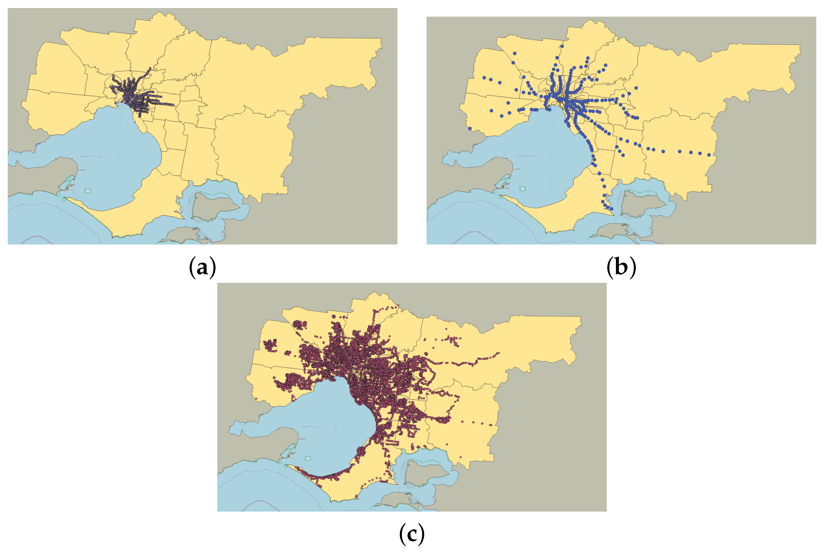
Figure 1.
Trains, trams, and buses within metropolitan Melbourne. (a) Tram lines; (b) train lines; (c) bus lines.
Figure 1.
Trains, trams, and buses within metropolitan Melbourne. (a) Tram lines; (b) train lines; (c) bus lines.
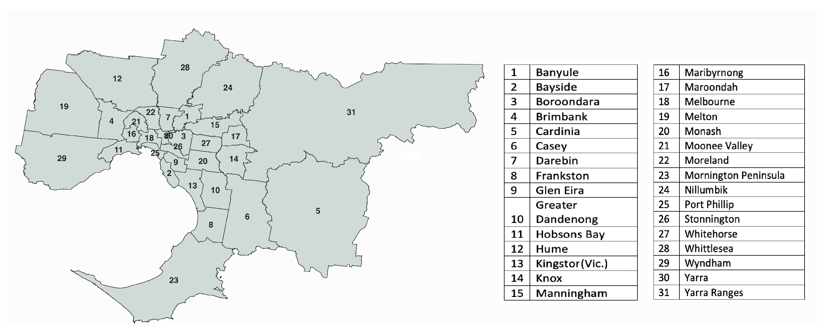
Figure 2.
Local government areas (LGAs) in metropolitan Melbourne.
Figure 2.
Local government areas (LGAs) in metropolitan Melbourne.
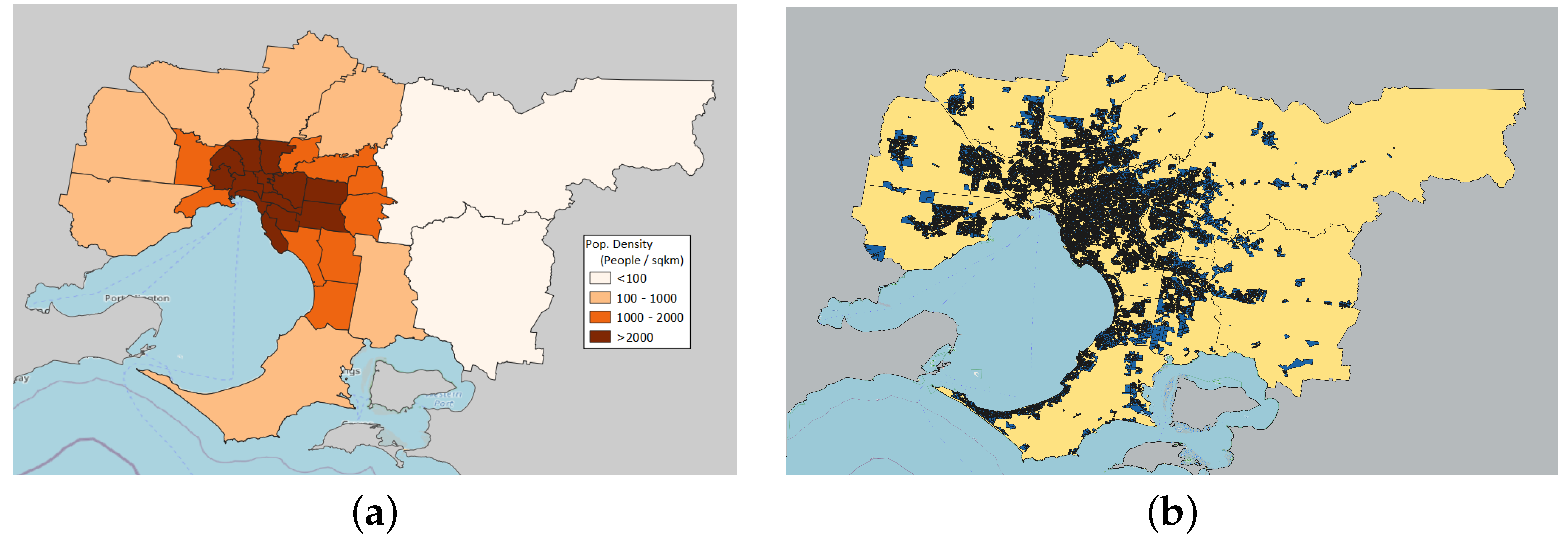
Figure 3.
The residential areas and populations in each LGA. (a) The population density based on LGA; (b) residential areas in metropolitan Melbourne.
Figure 3.
The residential areas and populations in each LGA. (a) The population density based on LGA; (b) residential areas in metropolitan Melbourne.
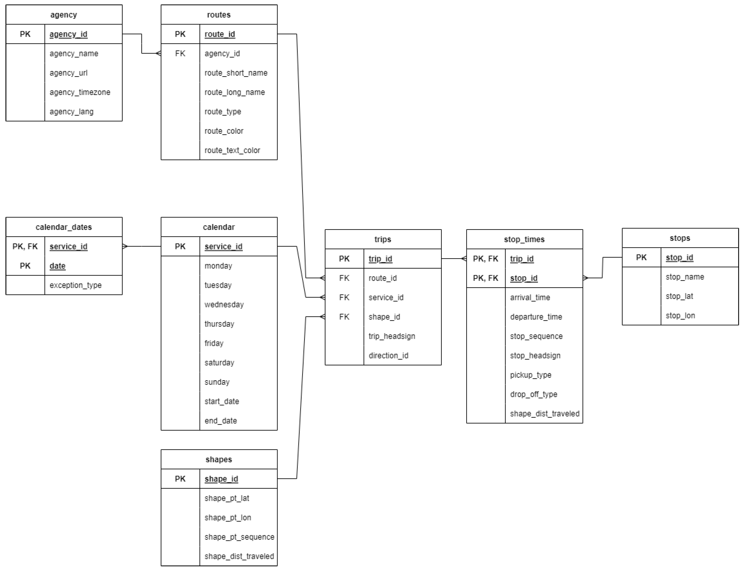
Figure 4.
GTFS entity relationship diagram.
Figure 4.
GTFS entity relationship diagram.
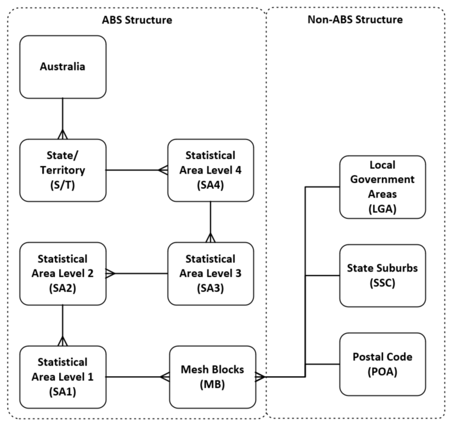
Figure 5.
Boundary structures in Australia.
Figure 5.
Boundary structures in Australia.
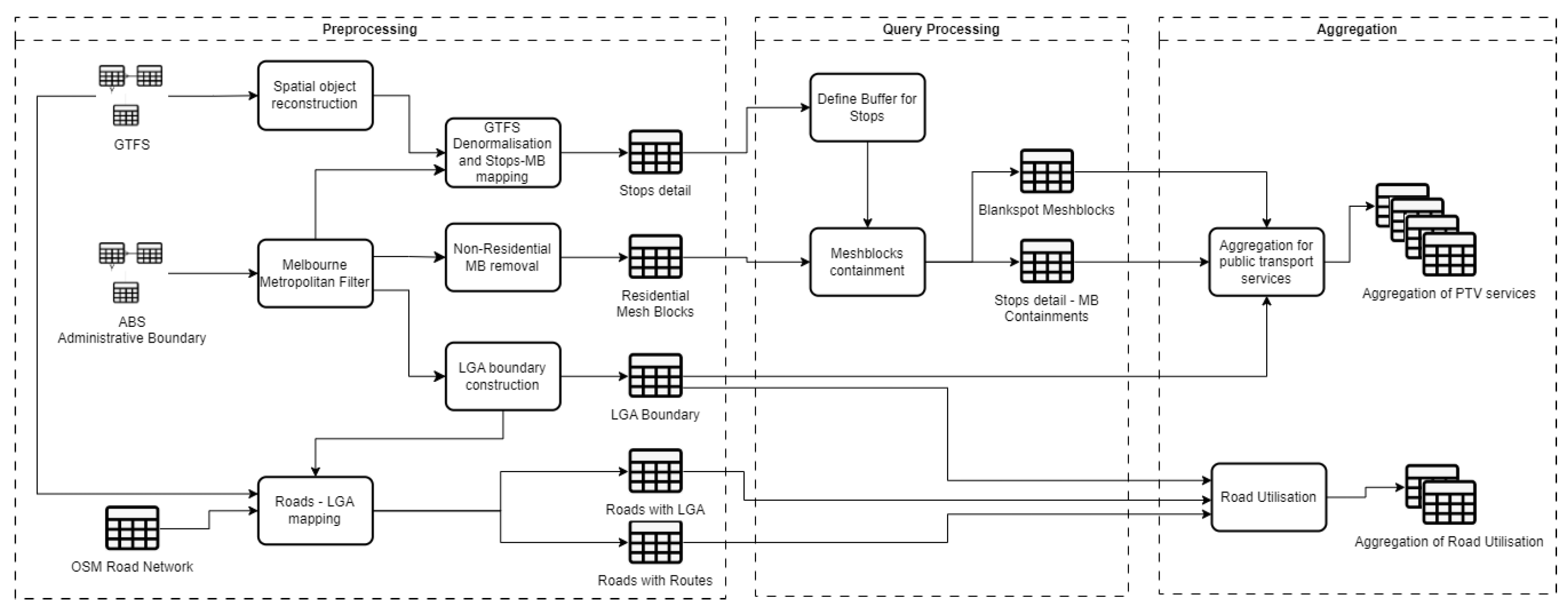
Figure 6.
The processing framework.
Figure 6.
The processing framework.
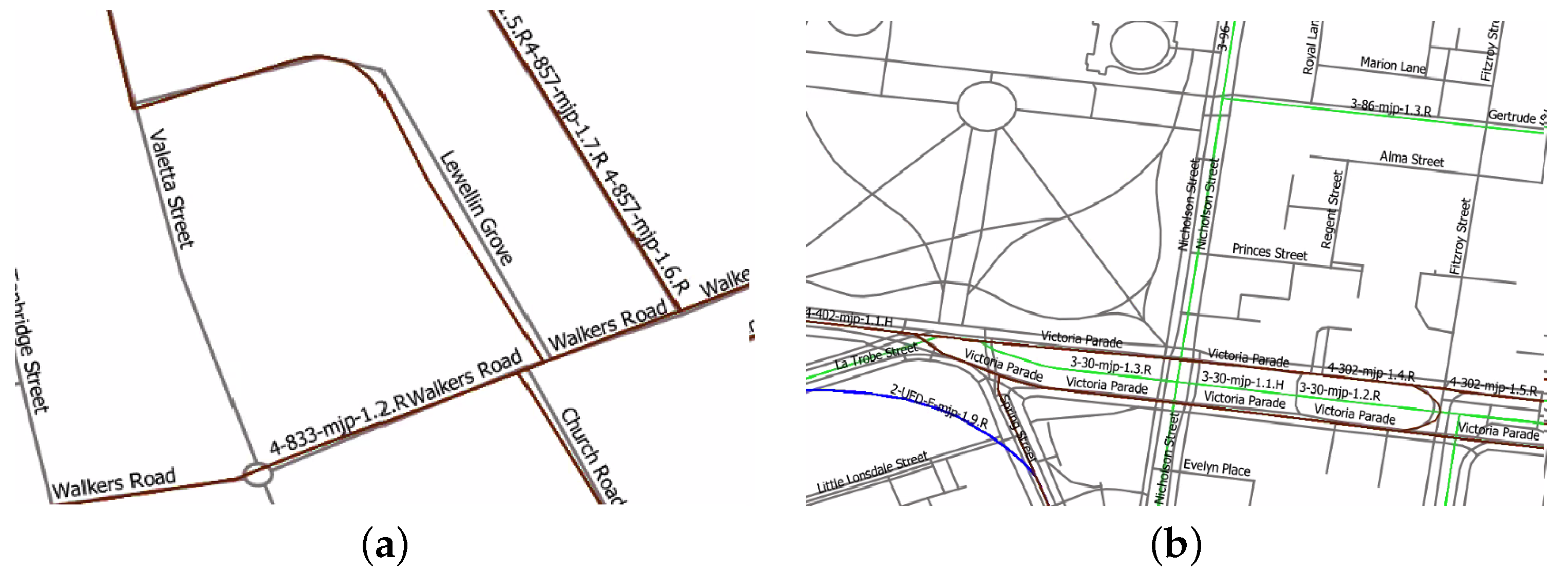
Figure 7.
Bus line (brown), tram line (green), train line (blue), and the road line (grey). (a) A bus line (brown) and road line (grey); (b) a tramline (green) and road line (grey).
Figure 7.
Bus line (brown), tram line (green), train line (blue), and the road line (grey). (a) A bus line (brown) and road line (grey); (b) a tramline (green) and road line (grey).
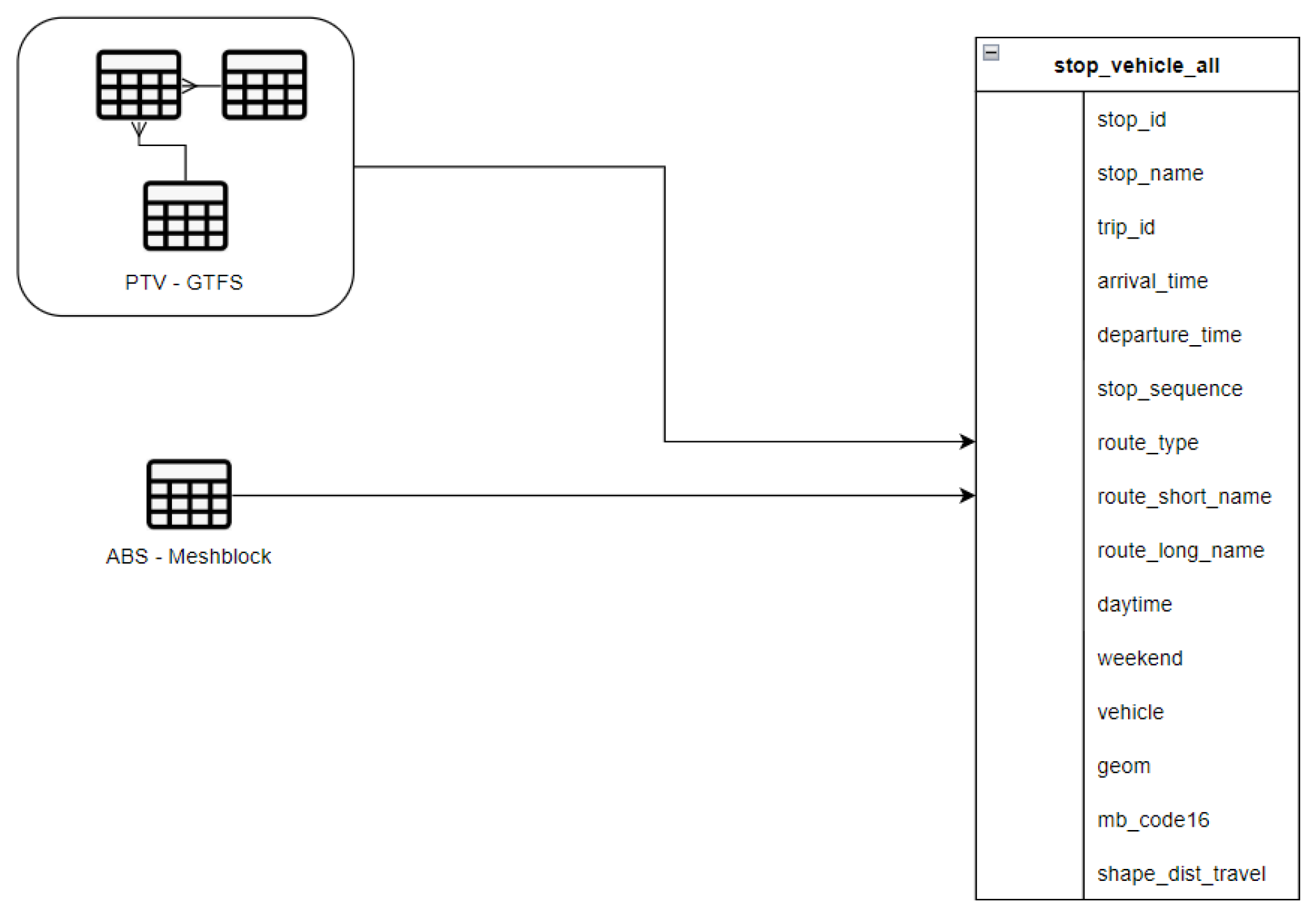
Figure 8.
GTFS denormalization.
Figure 8.
GTFS denormalization.
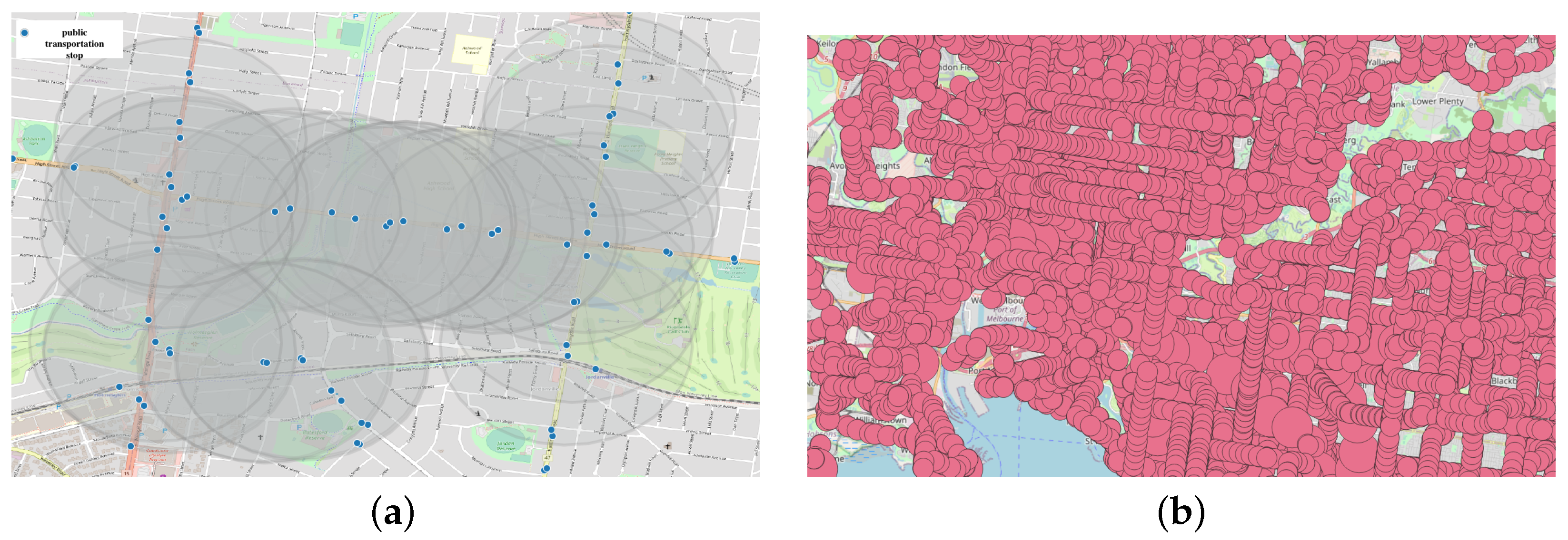
Figure 9.
Catchment analysis. (a) An example of the catchment in a suburb (400 m buffer for each pt stop); (b) a catchment for the whole of Melbourne (the buffers for each public transport stop).
Figure 9.
Catchment analysis. (a) An example of the catchment in a suburb (400 m buffer for each pt stop); (b) a catchment for the whole of Melbourne (the buffers for each public transport stop).
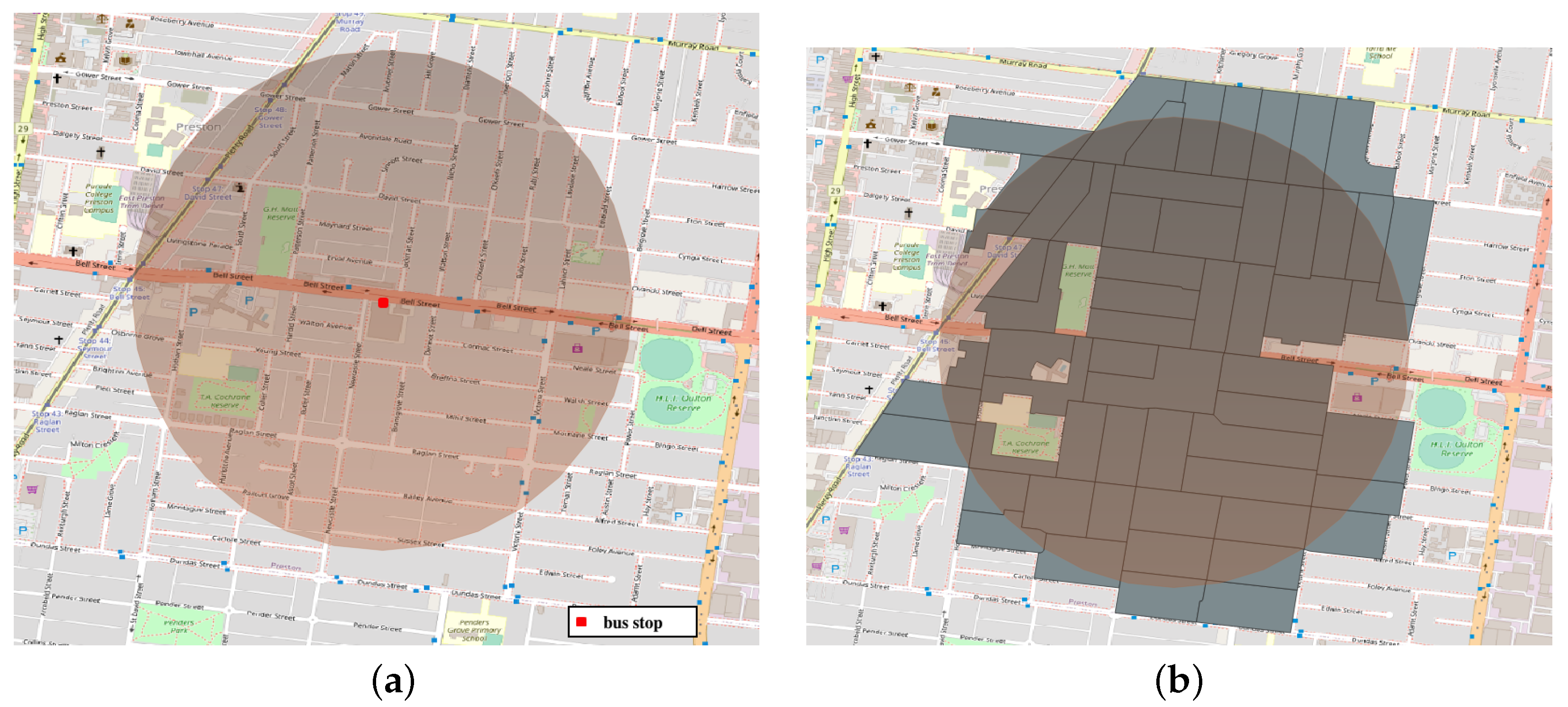
Figure 10.
One public transportation catchment example. (a) An example bus stop catchment (a buffer of 400 m); (b) a catchment that intersects with a mesh block.
Figure 10.
One public transportation catchment example. (a) An example bus stop catchment (a buffer of 400 m); (b) a catchment that intersects with a mesh block.
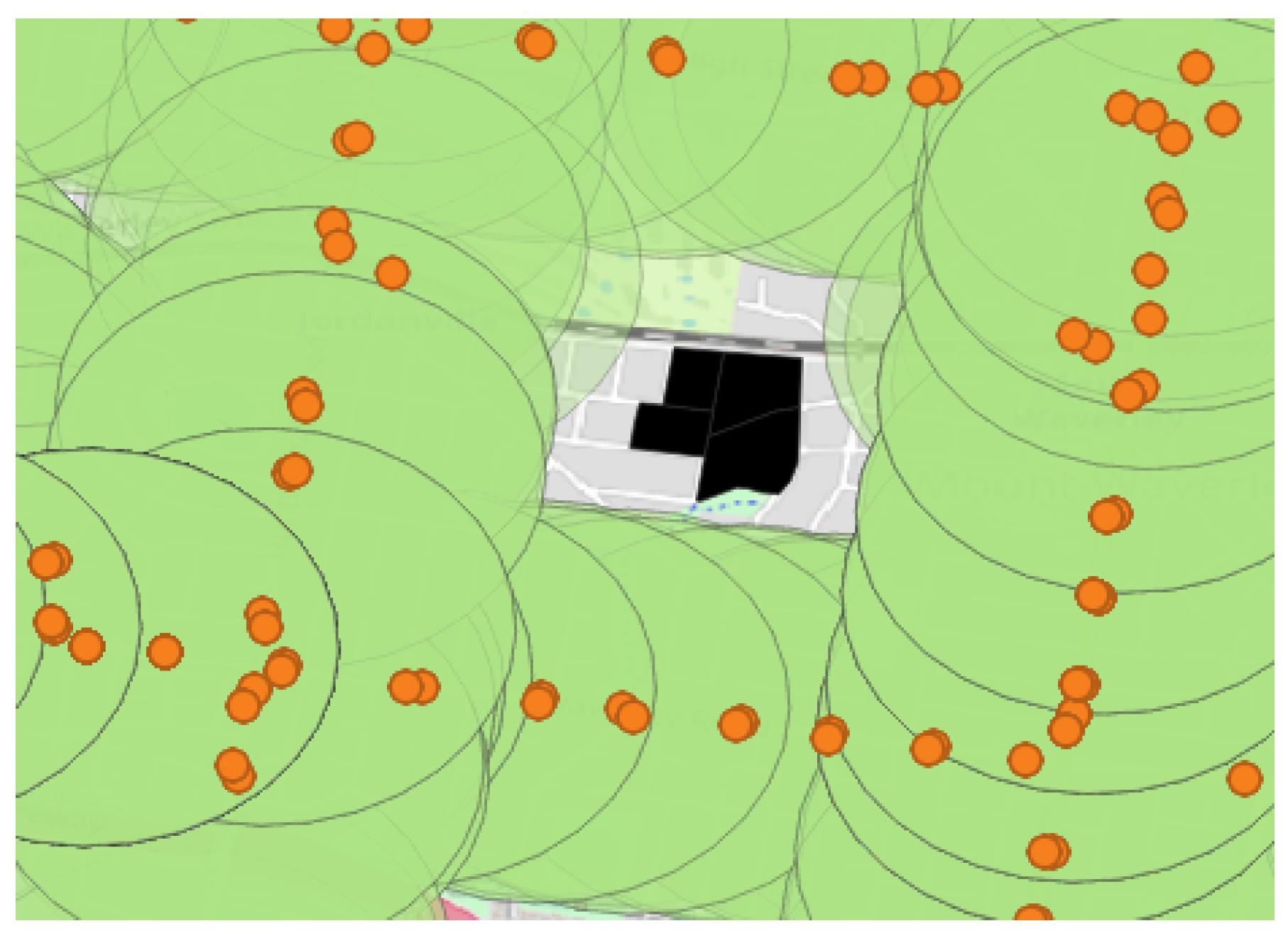
Figure 11.
An example of blank spot verification between catchments.
Figure 11.
An example of blank spot verification between catchments.
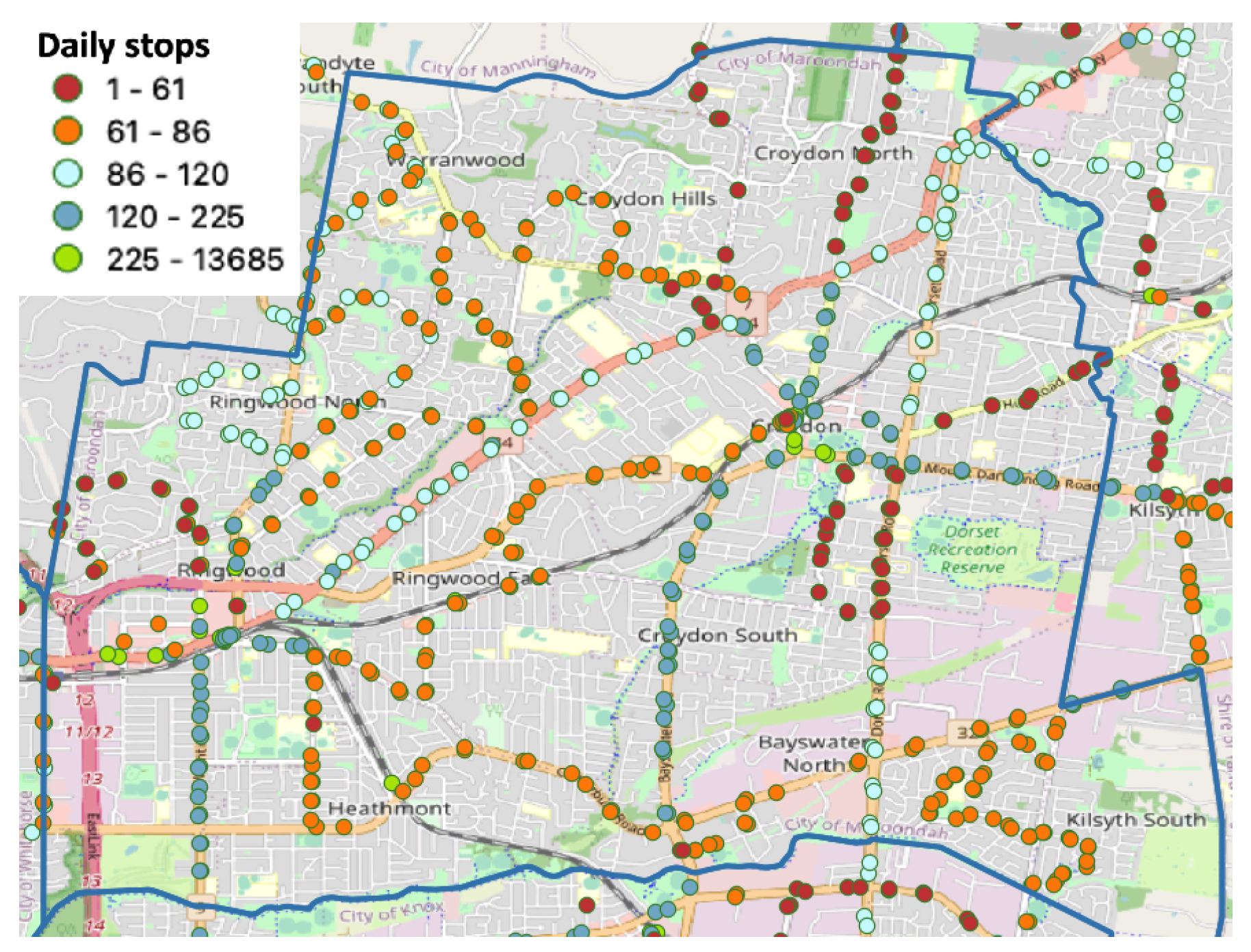
Figure 12.
Maroondah City PT daily stops.
Figure 12.
Maroondah City PT daily stops.
Figure 13.
Blank spots within metropolitan Melbourne. (a) Percentage of blank spots in each LGA; (b) blank spots.
Figure 13.
Blank spots within metropolitan Melbourne. (a) Percentage of blank spots in each LGA; (b) blank spots.
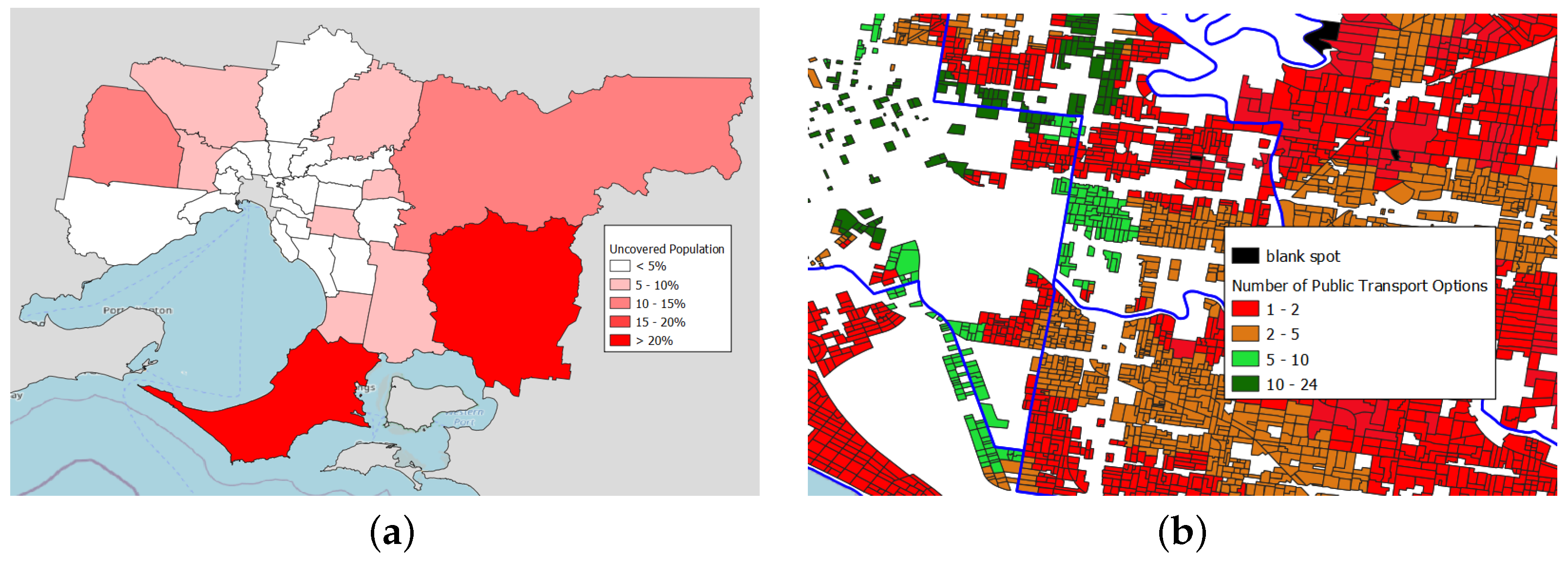
Figure 14.
The blank spots of the Melbourne metropolitan area. (a) Uncovered population; (b) MB catchment and LGA.
Figure 14.
The blank spots of the Melbourne metropolitan area. (a) Uncovered population; (b) MB catchment and LGA.
Figure 15.
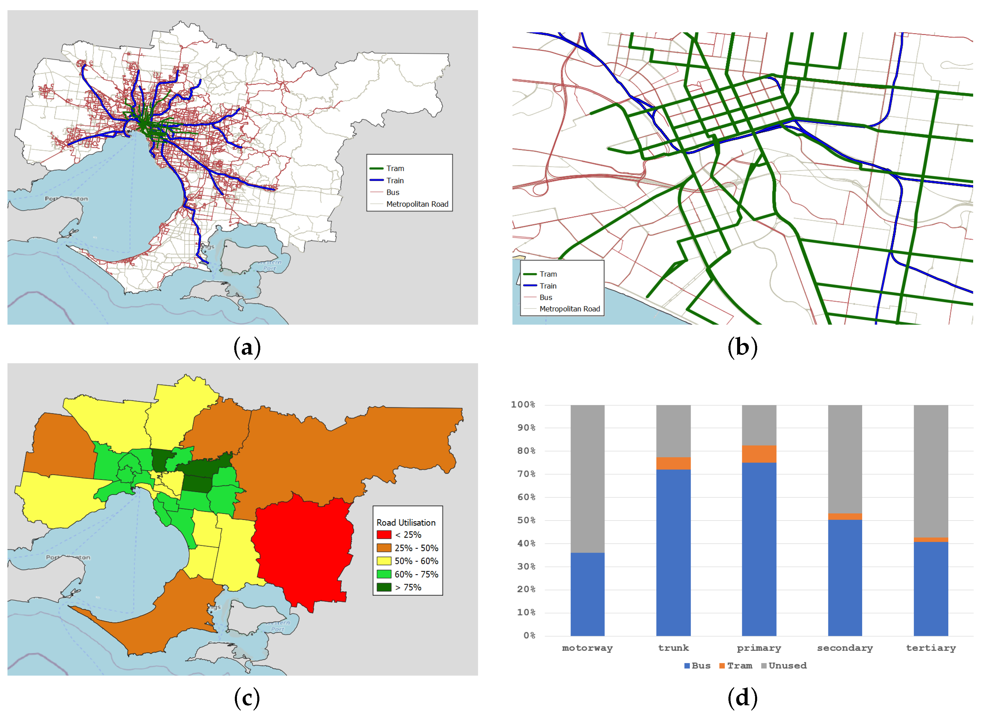
Roads utilized by public transport vehicles. (a) PTV and road network; (b) example PTV network in CBD; (c) road utilization by LGA; (d) road utilization by OSM road type.
Figure 15.
Roads utilized by public transport vehicles. (a) PTV and road network; (b) example PTV network in CBD; (c) road utilization by LGA; (d) road utilization by OSM road type.
Figure 16.
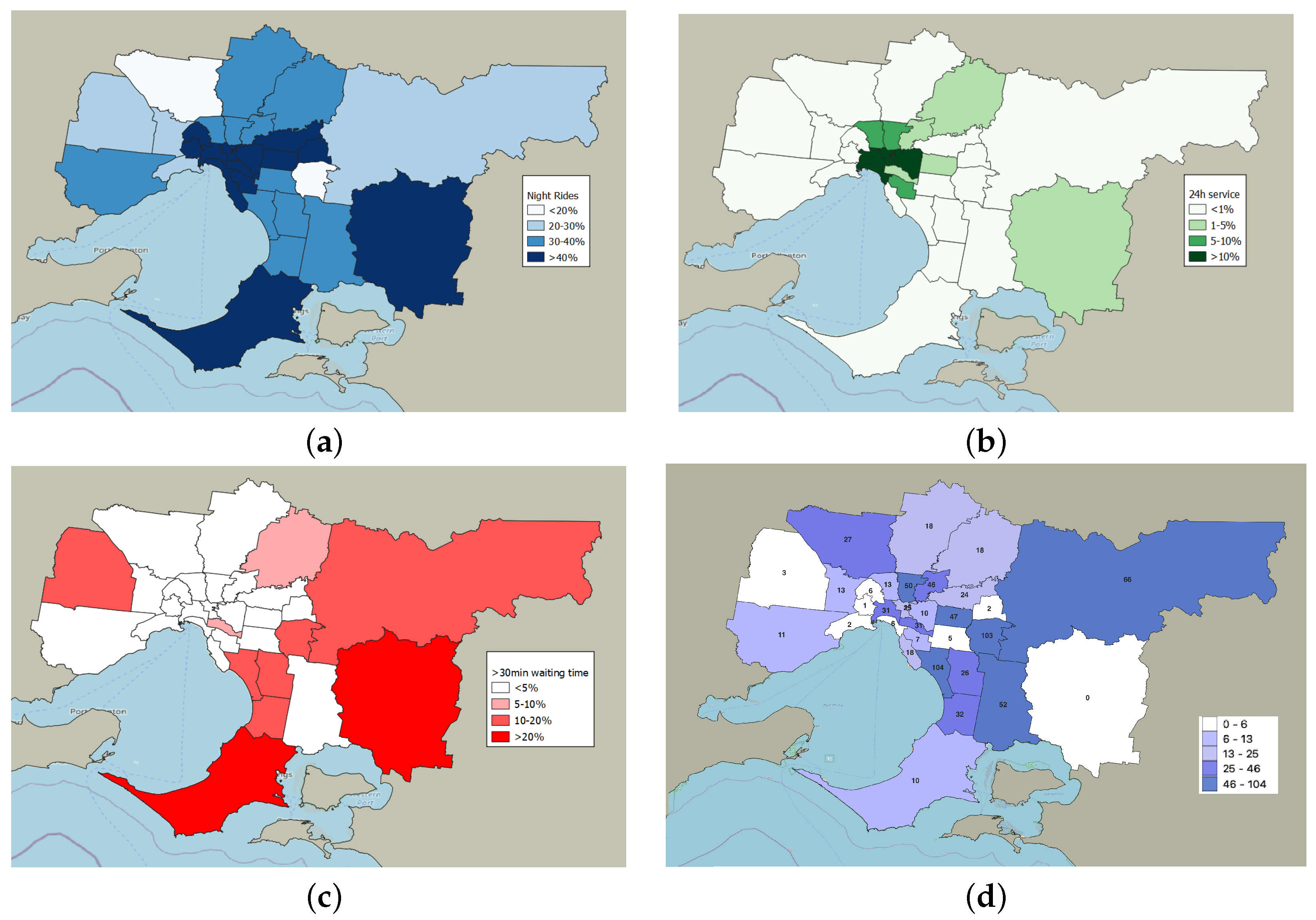
The availability of public transportation in Melbourne metropolitan area from different aspects. (a) Night rides; (b) 24-h availability; (c) active interval; (d) weekend availability.
Figure 16.
The availability of public transportation in Melbourne metropolitan area from different aspects. (a) Night rides; (b) 24-h availability; (c) active interval; (d) weekend availability.
Figure 17.
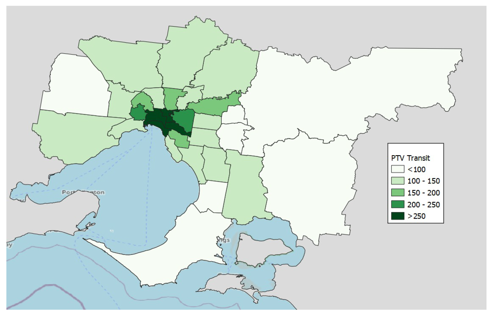
Stop transit average in each LGA.
Figure 17.
Stop transit average in each LGA.
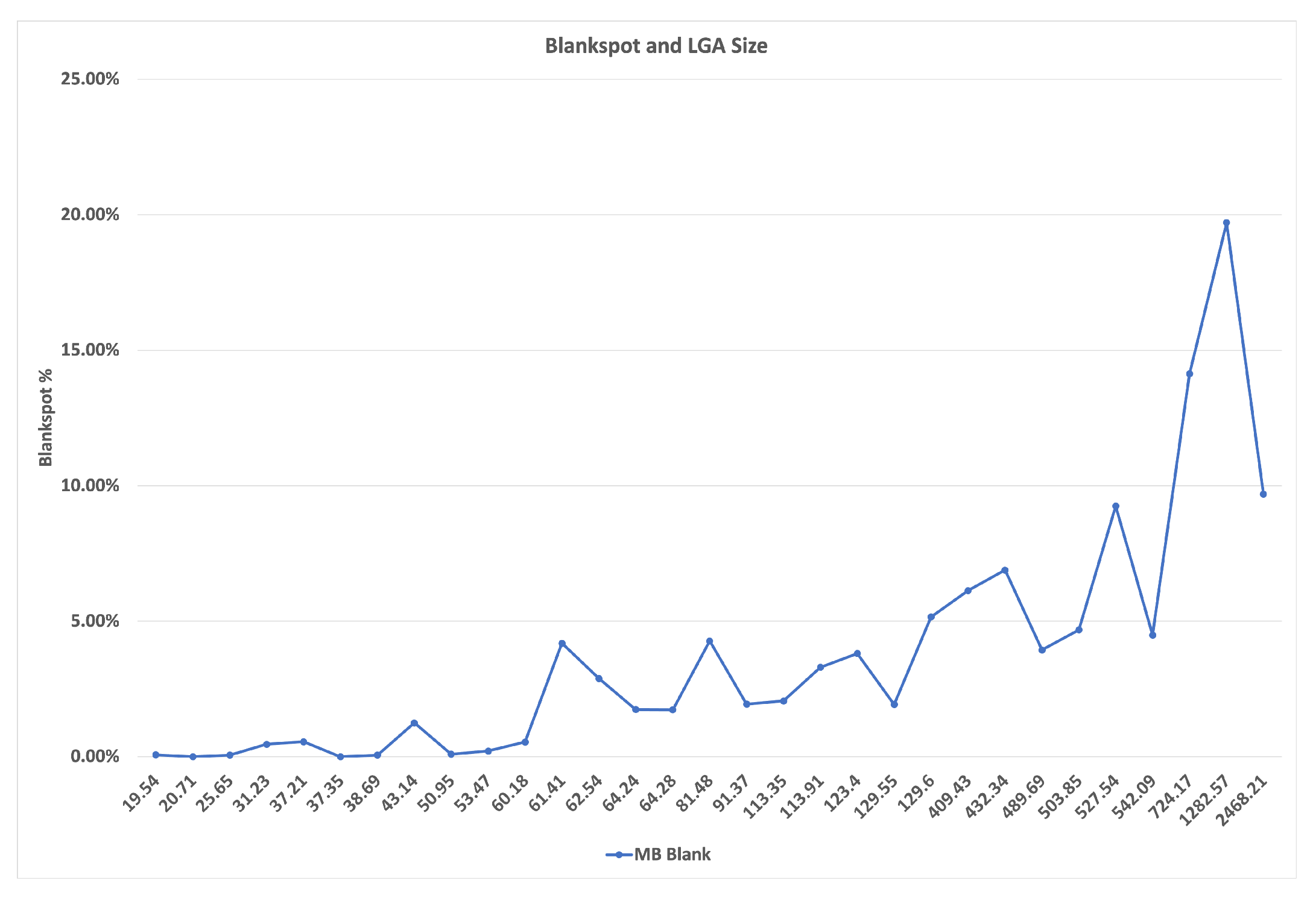
Figure 18.
Blank spots and the size of the LGA area.
Figure 18.
Blank spots and the size of the LGA area.
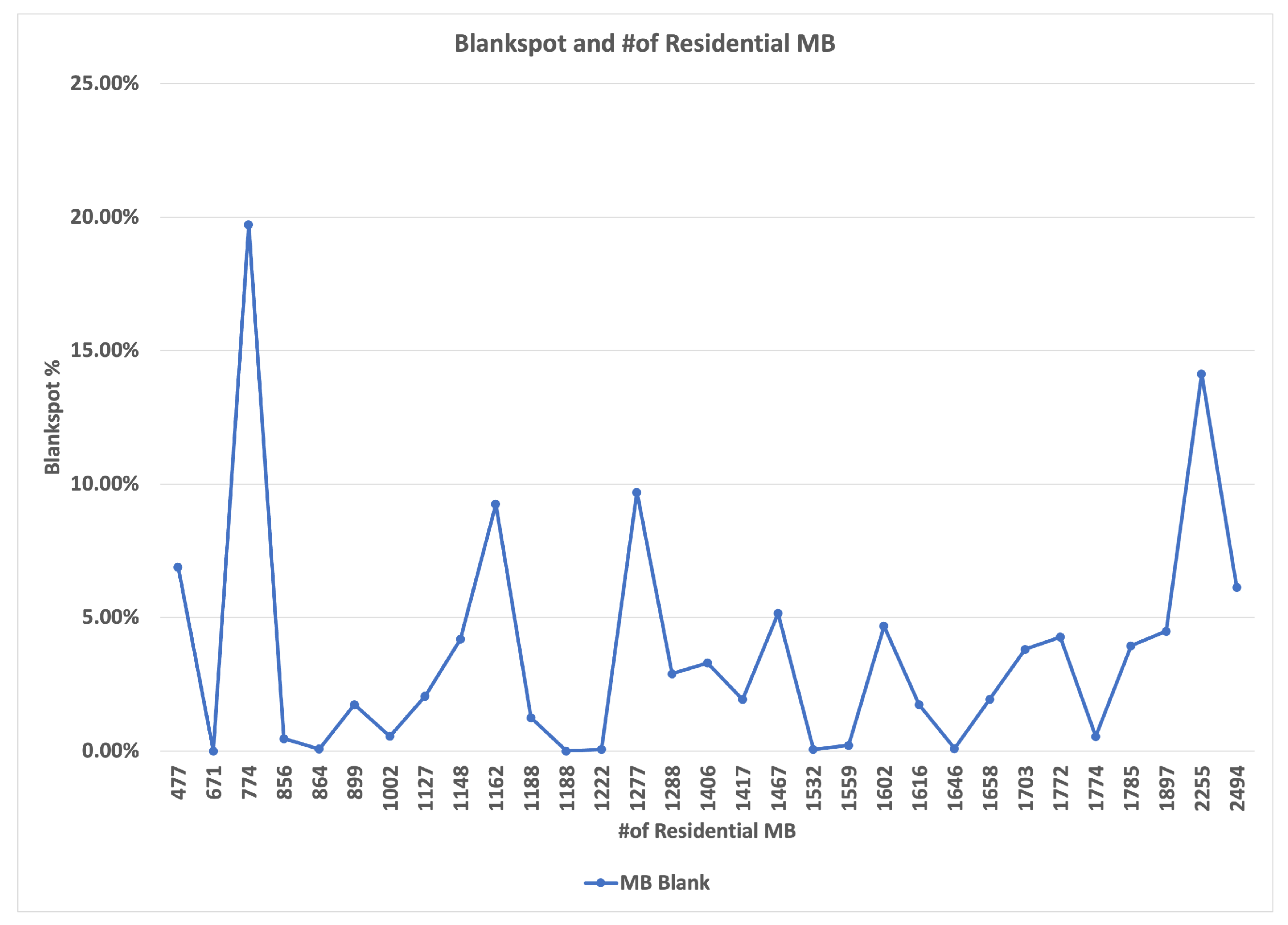
Figure 19.
Blank spots and number of residential MBs.
Figure 19.
Blank spots and number of residential MBs.
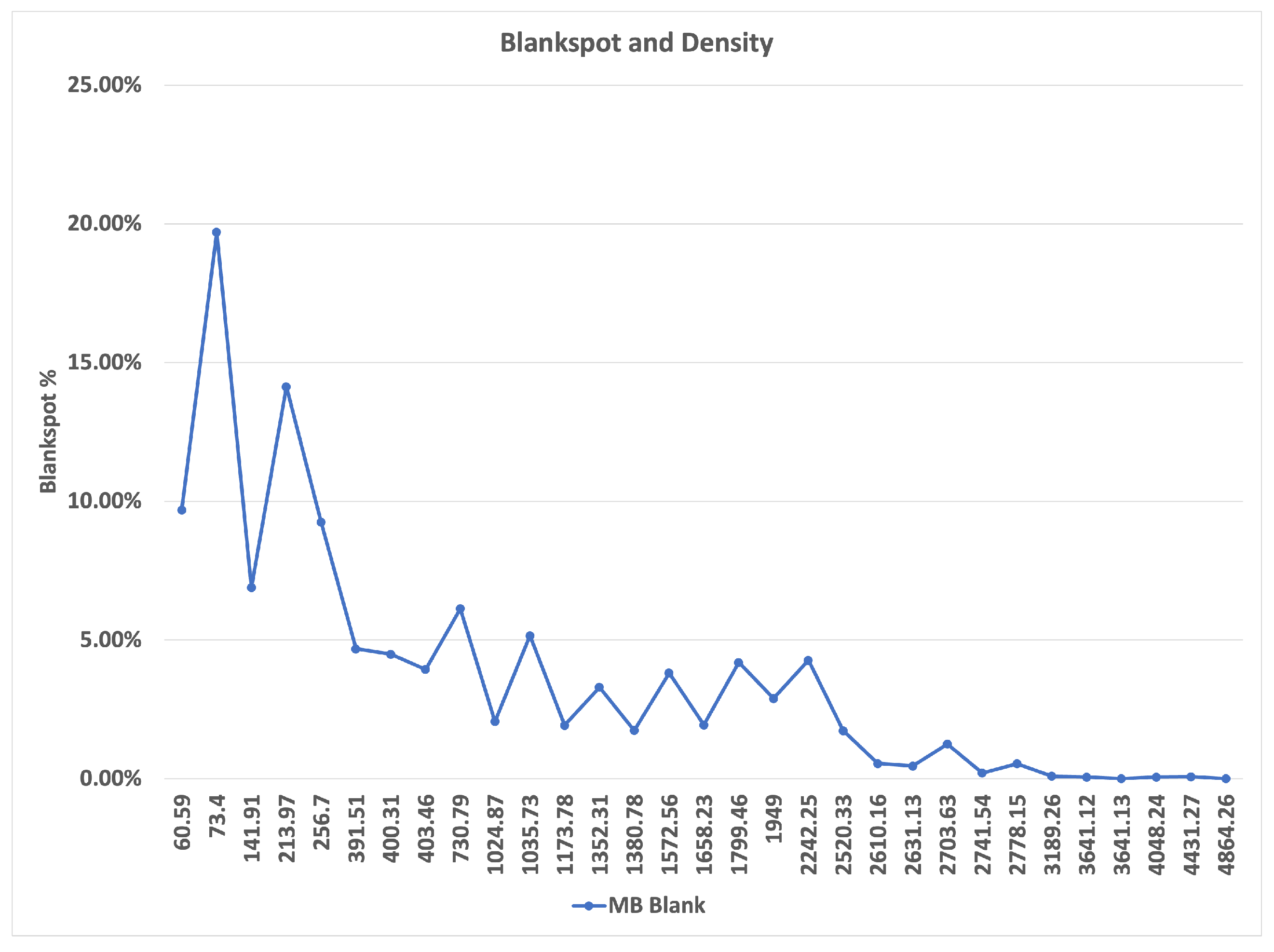
Figure 20.
Blank spots and LGA density.
Figure 20.
Blank spots and LGA density.
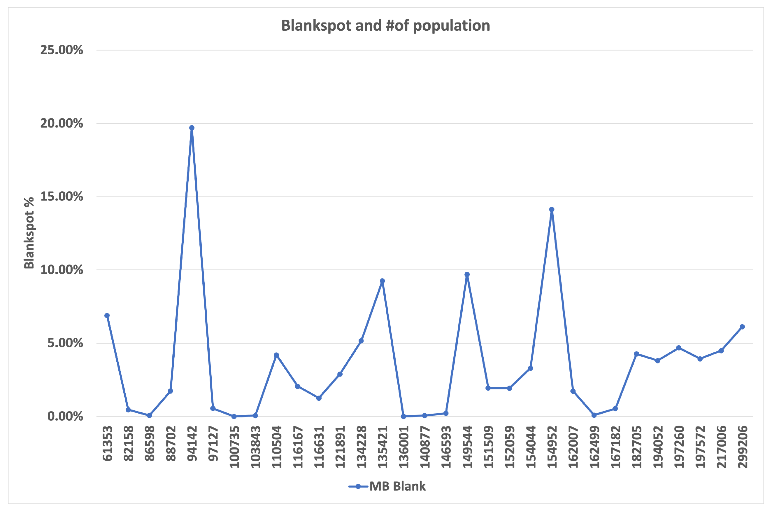
Figure 21.
Blank spots and the population.
Figure 21.
Blank spots and the population.
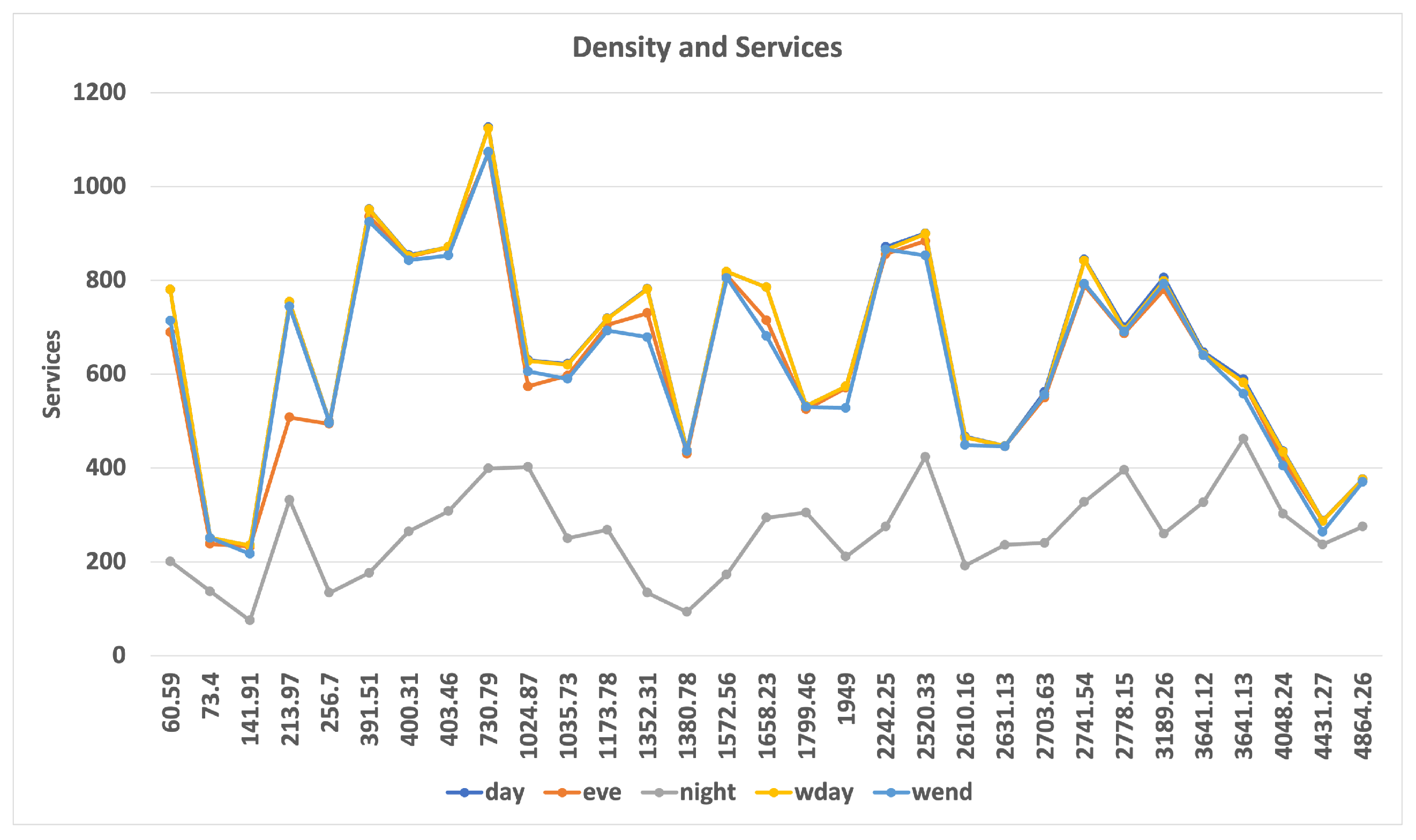
Figure 22.
Services and LGA density.
Figure 22.
Services and LGA density.
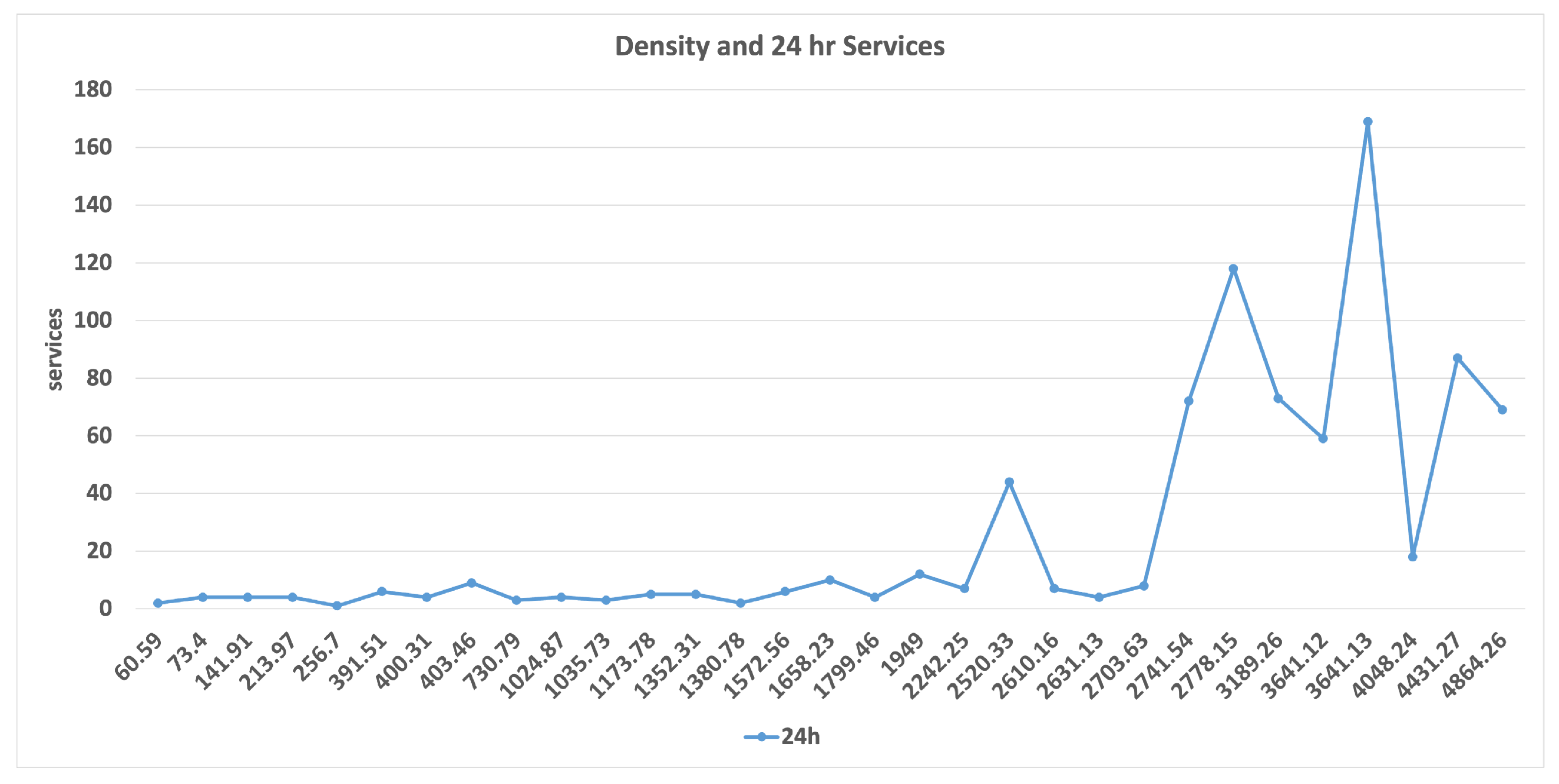
Figure 23.
LGA density and 24-h services.
Figure 23.
LGA density and 24-h services.
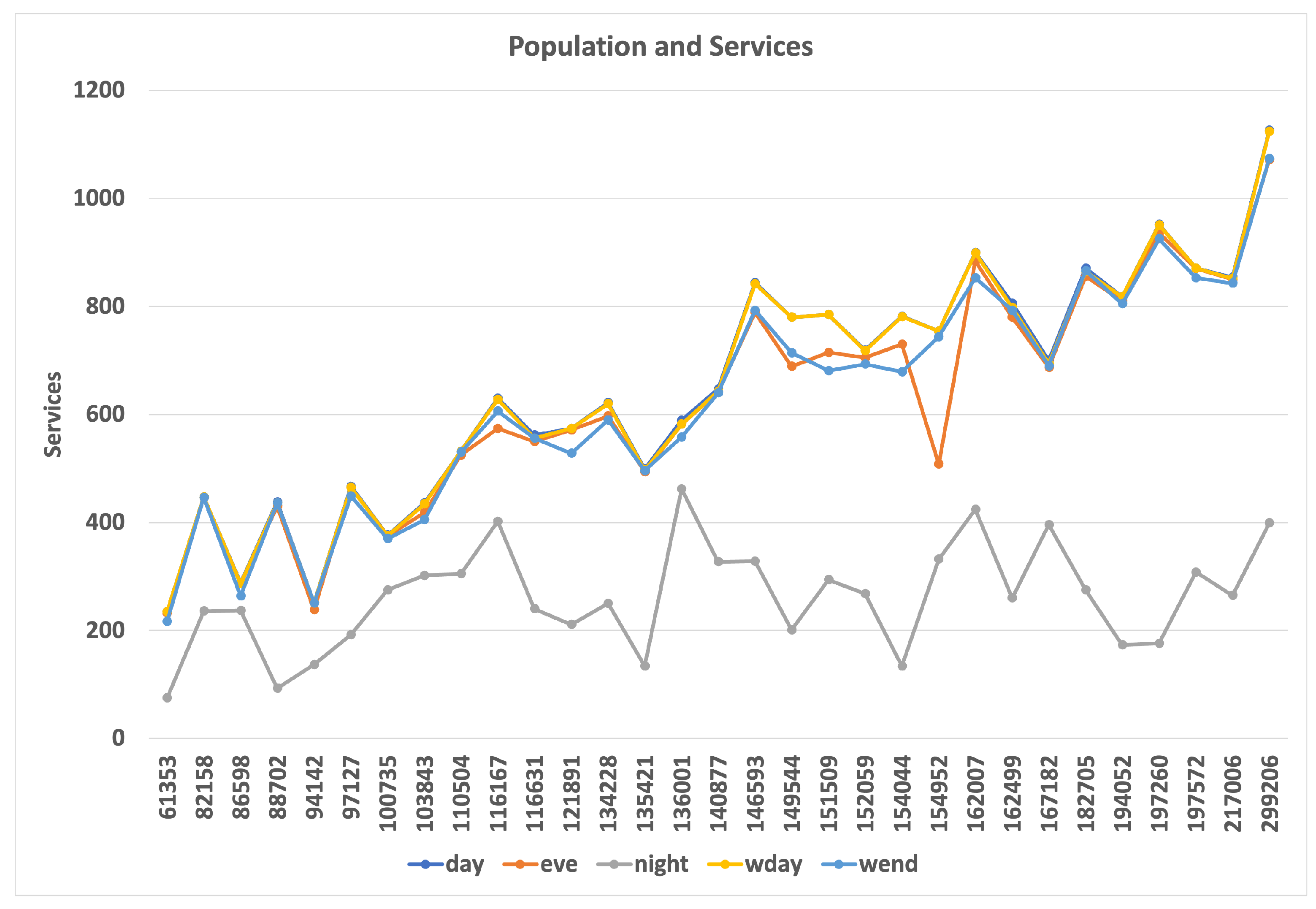
Figure 24.
Population and services.
Figure 24.
Population and services.
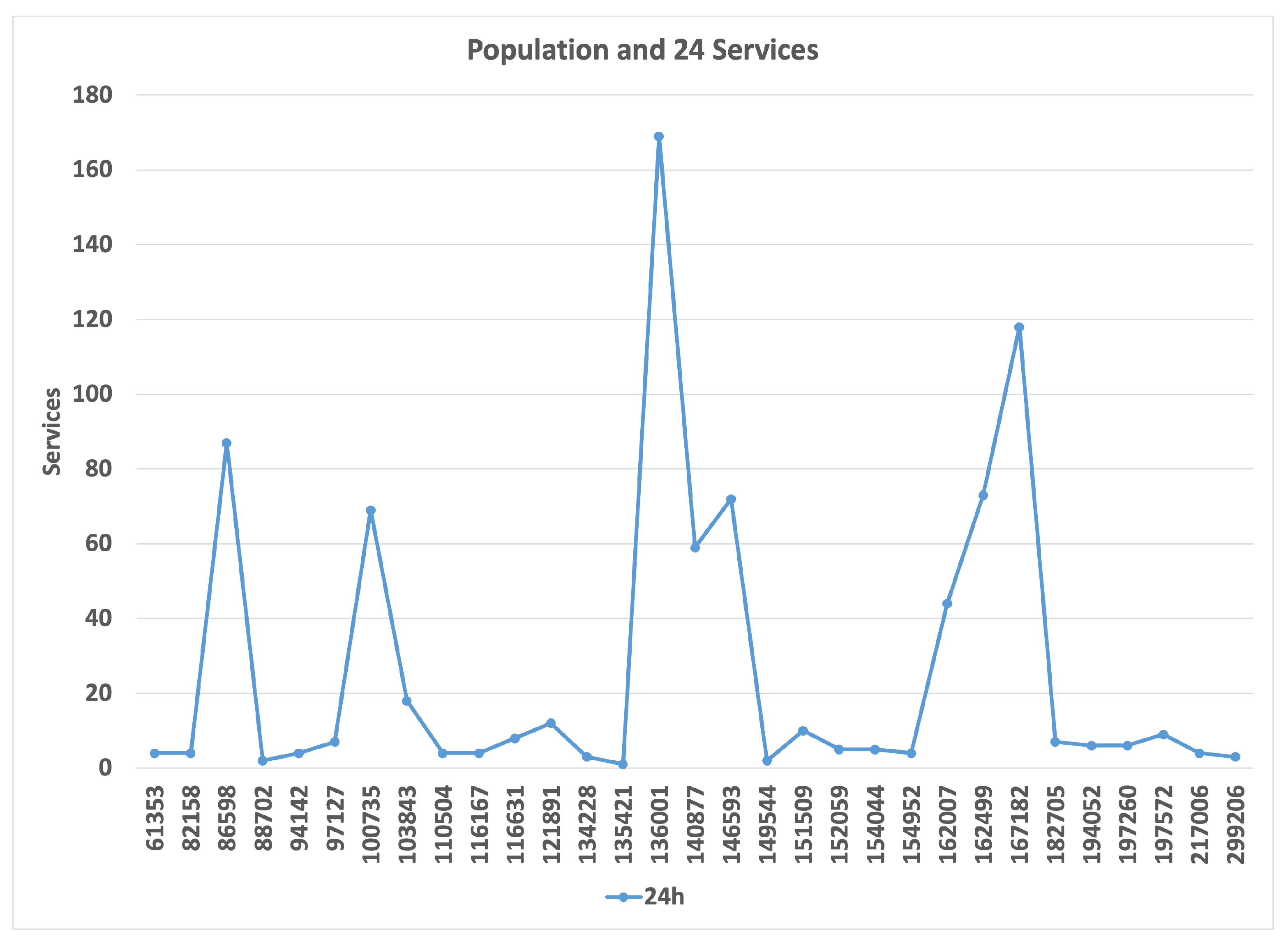
Figure 25.
Population and 24-h services.
Figure 25.
Population and 24-h services.
Figure 26.
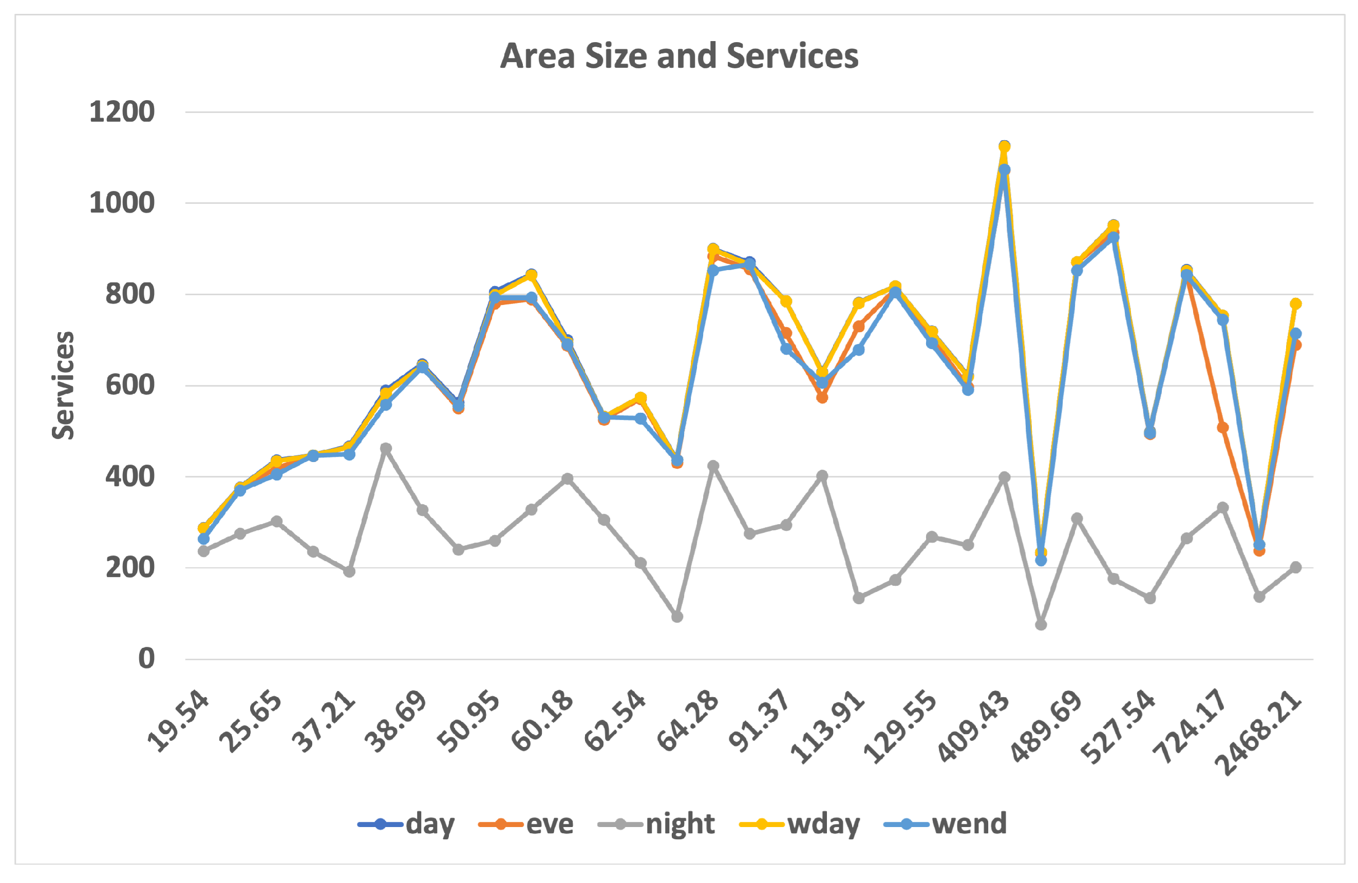
Services and LGA size.
Figure 26.
Services and LGA size.
Table 1.
Blank spots by category.
Table 1.
Blank spots by category.
| Category | Total | Blank | Percentage |
|---|
| Industrial | 1608 | 122 | 7.59% |
| Commercial | 3123 | 19 | 0.61% |
| Residential | 42,726 | 2173 | 5.09% |
| Hospital/Medical | 148 | 4 | 2.70% |
| Education | 1305 | 56 | 4.29% |
Table 2.
Road utilization by OSM type.
Table 2.
Road utilization by OSM type.
| Road Type | Length (km) | Bus (km) | Tram (km) | Unused (km) |
|---|
| Motorway | 1208 | 435 | 0 | 772 |
| Trunk | 901 | 649 | 49 | 203 |
| Primary | 1588 | 1191 | 121 | 277 |
| Secondary | 2131 | 1072 | 60 | 999 |
| Tertiary | 4017 | 1632 | 81 | 2304 |


