Article

Assessment of Perceived and Physical Walkability Using Street View Images and Deep Learning Technology

1
Department of Social Studies (Geography), Ewha Womans University, Seoul 03760, Republic of Korea
2
Department of Big Data Analytics, Ewha Womans University, Seoul 03760, Republic of Korea
*
Author to whom correspondence should be addressed.
ISPRS Int. J. Geo-Inf. 2023, 12(5), 186; https://doi.org/10.3390/ijgi12050186
Submission received: 9 February 2023 / Revised: 17 April 2023 / Accepted: 1 May 2023 / Published: 2 May 2023
(This article belongs to the Special Issue Urban Geospatial Analytics Based on Crowdsourced Data)

Abstract

:
As neighborhood walkability has gradually become an important topic in various fields, many cities around the world are promoting an eco-friendly and people-centered walking environment as a top priority in urban planning. The purpose of this study is to visualize physical and perceived walkability in detail and analyze the differences to prepare alternatives for improving the neighborhood’s walking environment. The study area is Jeonju City, one of the medium-sized cities in Korea. For the evaluation of perceived walkability, 196,624 street view images were crawled and 127,317 pairs of training datasets were constructed. After developing a convolutional neural network model, the scores of perceived walkability are predicted. For the evaluation of physical walkability, eight indicators are selected, and the score of overall physical walkability is calculated by combining the scores of the eight indicators. After that, the scores of perceived and physical walkability are visualized, and the difference between them is analyzed. This study is novel in three aspects. First, we develop a deep learning model that can improve the accuracy of perceived walkability using street view images, even in small and medium-sized cities. Second, in analyzing the characteristics of street view images, the possibilities and limitations of the semantic segmentation technique are confirmed. Third, the differences between perceived and physical walkability are analyzed in detail, and how the results of our study can be used to prepare alternatives for improving the walking environment is presented.

1. Introduction

Neighborhood walkability is an important topic in various fields such as urban planning, health, and transportation. The walking environment is assessed as one of the critical factors for creating a sustainable city because it helps improve public health [1,2,3], increases community bonds [4,5], contributes to community development [6,7], alleviates traffic congestion, and reduces carbon emissions along with green transportation [8,9]. With the growing awareness that neighborhood walkability greatly affects our lives, many cities around the world are promoting an eco-friendly and people-centered walking environment as the top priority in urban planning [10,11,12,13]. Moreover, in Korea, the pedestrian rights movement began in the 1990s under the slogan ‘Creating a Walkable City’, and the Ministry of Public Administration and Security enacted a related law to promote the walking environment in 2012 [14]. Every five years, local governments across the country establish a basic plan and conduct a survey on pedestrian safety and convenience enhancement.
As the importance of neighborhood walkability increases, a number of studies in the field of urban planning have identified the characteristics of the neighborhood environment. The studies showed that residents’ walking increased in urban residential areas with high residential density, a good land use mix, small block sizes, and good street connectivity [15,16,17,18]. Early studies on the walking environment focused on the physical design features of neighborhoods. However, as it has been known that perceived walkability is as important as physical design features, several studies have been performed to analyze what kind of walking environment people are satisfied with [19,20,21].
From a data analysis point of view, as the available data have increased and the GIS analysis technique has improved, studies have subdivided the indicators for assessing physical walkability and measured the walking environment at the mesoscale [22]. On the other hand, other studies have assessed the perceived walkability with a survey or on-site participant questionnaire targeting some areas [20,23]. However, recently, street view images (SVIs) provided by the internet portal platform and computer vision technology have opened a new chapter in assessing the neighborhood walking environment. The SVI and deep learning technology enable the assessment of physical walkability in detail by automatically extracting a variety of information. In addition, a more realistic assessment is possible by showing SVI and asking how good the point is for walking in the assessment of perceived walkability [24].
However, current research on both physical and perceived walkability assessments has certain limitations. The application of SVIs and semantic segmentation technology to evaluate physical walkability is limited by the lack of a detailed analysis of the accuracy and problems of semantic segmentation results. Perceived walkability assessment studies have limitations when using pairwise comparison training datasets due to the time-consuming and difficult process of obtaining a large number of responses. Additionally, previously published models such as SS-CNN or RSS-CNN are not suitable for small and medium-sized cities, necessitating the development of a new deep learning model to improve accuracy. As such, further research is needed to overcome these limitations and improve the accuracy of walkability assessments.
The purpose of this study is to assess the perceived and physical walkability of a small and medium-sized city, Jeonju, in Korea. Additionally, we analyze the differences between them. For detailed analysis, we used the semantic segmentation technique of SVIs for physical walkability, constructed a pairwise comparison dataset, and developed a deep learning model for perceived walkability.

2. Literature Review

2.1. Studies on the Walking Environment

A variety of studies have assessed the neighborhood’s walking environment and recognized the importance of walkability. Frank et al. [25] revealed that the better the physical design features of neighborhoods, such as residential density, land use mix, and street network connectivity, the more pedestrian activity there is. Lee and Ahn [26] found that the frequency of walking activities was high both when the land-use mix was high and nearby living facilities such as walking, exercise, and shopping were good. In most studies analyzing the physical characteristics of the walking environment, key factors that affected walking, such as pedestrian comfort, safety, street diversity, street connectivity, and public transport accessibility, were extracted through surveys or site visits [20,22,27,28,29,30].
Unlike the existing studies based on a survey or site visits, new approaches, which assess the physical walking environment by applying the semantic segmentation technique to the street view image, are evolving recently. Zhou et al. [31] measured visual walkability using Baidu SVIs in Shenzhen. They created four visual walkability indexes: psychological greenery, visual crowdedness, outdoor enclosure, and visual pavement. In addition, they calculated the score of Integrated Visual Walkability (IVW) and found that the IVW was uneven in space. Li et al. [32] developed Walkability on Urban Street (WoUS), which was composed of seven indicators and focused on the area around Osaka University in Japan. The seven indicators were walk score, pedestrian flow density, noise, light, greenery, enclosure, and relative walking width. Among them, greenery, enclosure, and relative walking width were calculated by segmenting street view images. By comprehensively analyzing seven scores, they visualized WoUS by street and compared physical WoUS with perceived WoUS obtained by an expert questionnaire. Wu et al. [33] analyzed SVIs in Shenzhen using semantic segmentation techniques and confirmed that the importance of objects varied according to spatial scale. On the other hand, Li and Latti [34] developed the sky view factor (SVF) and green view index (GVI) by analyzing the physical characteristics of the street view image. By applying SVF and GVI, they confirmed that the correlation between street landscape characteristics and pedestrian activity was different for each type of land use.
The recent development of SVIs and semantic segmentation technology is expanding the possibility of including not only GIS data but also various objects obtained from SVIs in the assessment of the physical walking environment. However, there is a limitation in that the accuracy and problems of the semantic segmentation result of the SVIs have not been analyzed in detail.

2.2. Assessment of Perceived Walkability Using Deep Learning Technology

Along with the study to understand the physical features that made up the neighborhood walking environment, other studies analyzed what kind of walking environment people felt was good for walking [18,19,20,35,36,37]. As studies to analyze perceived walkability, Park et al. [36] revealed that street comfort was the greatest factor that affected walking satisfaction, and Mateo-Babiano [20] found that mobility, safety, ease, accessibility, and pleasure were the main factors in satisfying pedestrians. However, the survey on the perceived walkability of residents showed limitations in representativeness because field surveys are usually conducted by targeting some residents in small areas.
Meanwhile, as Google has started a street view service and computer vision technology has developed rapidly, a new approach to analyzing people’s perceptions of urban built environments, such as sentiment [38,39], walking environment [31,32,40], greenery [34], etc., is emerging. Unlike aerial photography or satellite imagery, the SVIs are suitable for evaluating people’s perceptions of the urban built environment because they enable examining visual features from a human perspective [41,42]. The Place Pulse dataset served as an opportunity to promote studies to qualitatively assess urban built environments using SVIs.
The media lab at MIT University in the U.S. has built a website that can conduct a survey on urban landscapes based on SVIs. The volunteers who visited the website were asked to select the superior one from two SVIs from a specific point of view, such as safety, liveliness, and beauty. Place Pulse is a dataset that has been built and published with this response result. Place Pulse 1.0 is a data set constructed as a result of 200,000 pairwise comparisons of 4109 images collected from New York and Boston (U.S.) and Linz and Salzburg (Austria) [38]. In addition, Place Pulse 2.0 is a dataset that expanded version 1.0 and built 1.17 million pairwise comparison results as a database using 110,988 images collected from 56 cities in 28 countries. The dataset of Place Pulse 1.0 provides pairwise comparison data for three emotions, while the dataset of Place Pulse 2.0 provides pairwise comparison results for six emotions: ‘Which place looks safer, livelier, more beautiful, richer, gloomier, or more boring?’. A deep learning model using pairwise comparison datasets has also been activated. Using Place Pulse 2.0 data, Dubey et al. [39] proposed a convolutional neural network (CNN) model that could predict pair-wise comparisons of perceptual properties when inputting pairs of images and named them street score-CNN (SS-CNN) and ranking SS-CNN (RSS-CNN), respectively. Since then, several studies have proposed a deep learning model architecture for predicting perceived sensibility using the Place Pulse dataset. However, as far as we know, there is currently no publicly available dataset that captures people’s preferences for walking environments through pairwise comparisons.
The architecture of the deep learning model predicting perceptions of the urban built environment can be divided into two types according to the method of collecting people’s perceptions. The first is to collect the perception of SVIs from respondents as absolute values [43,44]. Participants assign a score according to the Likert scale for a given street view image. Accordingly, the model is trained to predict the sentiment score using a single SVI as input data. However, these studies have limitations in terms of the reliability and accuracy of their scores. According to previous studies, it is relatively efficient and accurate to collect responses through a pairwise comparison of two images rather than to collect absolute scores for an image [45,46]. The second is to collect responses from pairwise comparisons between the two images. In this method, participants are presented with two SVIs and asked to choose one for a question, such as ‘Which one is more beautiful?’. Dubey et al. [39] proposed an SS-CNN and RSS-CNN model to evaluate street sentiment using Places Pulse 2.0. Since then, a number of studies have proposed a deep learning model for predicting urban sensibility using this dataset [47,48,49].
Deep learning models that assess people’s perceptions using pairwise comparison data have two characteristics. First, it has a model architecture based on the Siamese network. Koch et al. [50] proposed a Siamese network to learn the similarity between image vectors through two identical neural networks. The two neural networks receive different image vectors as inputs, but their weights are jointly updated because they are combined by the loss function at the top. Through shared weights, similar images can be embedded at nearby points in the vector space. As such, a Siamese network that learns the similarity and differences between two input data is suitable as a model structure using pairwise comparison data. Second, it uses a loss function to optimize ranking learning. A Rank support vector machine (RankSVM), RankBoost, and RankNet are used as models for learning ranking. A loss function is calculated as the matching ratio between the score of the actual input pair and the score predicted by the model.
From the perspective of perceived walkability assessment, existing studies [31,32,40] have limitations in two aspects. Firstly, using pairwise comparison training datasets is more accurate than using a single image’s absolute score, but building such a dataset is time-consuming and requires a significant amount of effort. In order to perform pairwise comparisons of a large number of images, it is necessary to build a dataset that can be compared more than K times for all comparison targets so that a stable score can be derived while ensuring an appropriate degree of accuracy [51,52,53]. Creating a web-based crowdsourcing site for pairwise comparison surveys and verifying the consistency of the responses requires a significant effort that goes beyond the scope of research in most walkability studies. Therefore, there is a scarcity of studies that utilize pairwise comparison data. Secondly, the previously published SS-CNN or RSS-CNN model uses the place pulse 2.0 data as the training data set, which may not be suitable for small and medium-sized cities where the differences in street scenery are not clear. Therefore, a new deep learning model is required to improve accuracy.

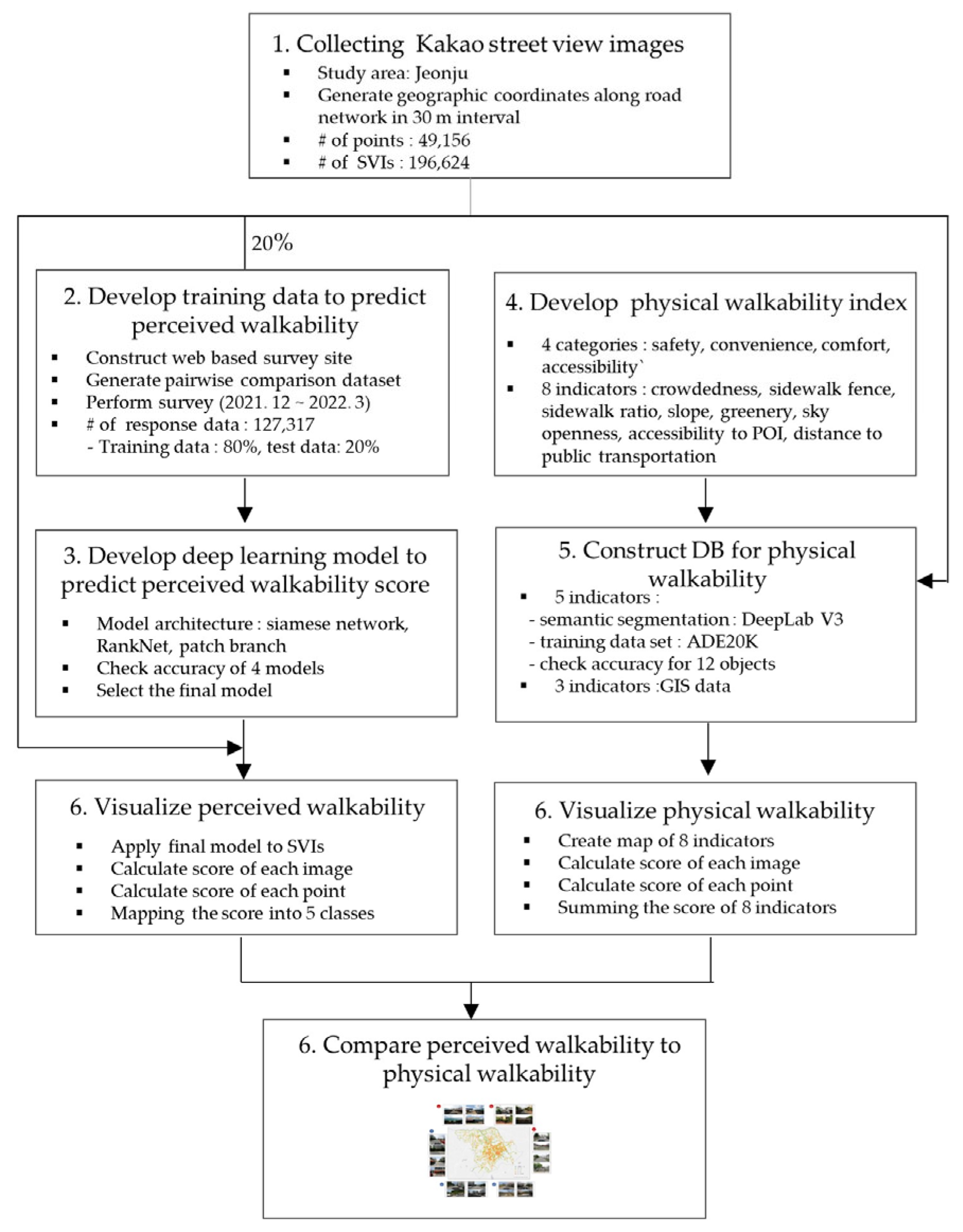
3. Materials and Methods

The study area for assessing walkability is Jeonju, a medium-sized city with a population of 650,000 located in the southwest of Korea. As a historical city that dates back to the Joseon Dynasty, Jeonju has a tourist attraction called Jeonju Han-ok Village, where you can experience lots of traditional elements. Jeonju has a provincial government office and city hall in the city center, and the old and new towns coexist. New residential areas have been formed on the outskirts of the city, and a little out of the city center is a rural area, as shown in Figure 1.
Figure 2 shows the research flow for assessing the walkability of Jeonju. Research procedures are as follows:
  • Step 1: collect the SVIs in Jeonju.
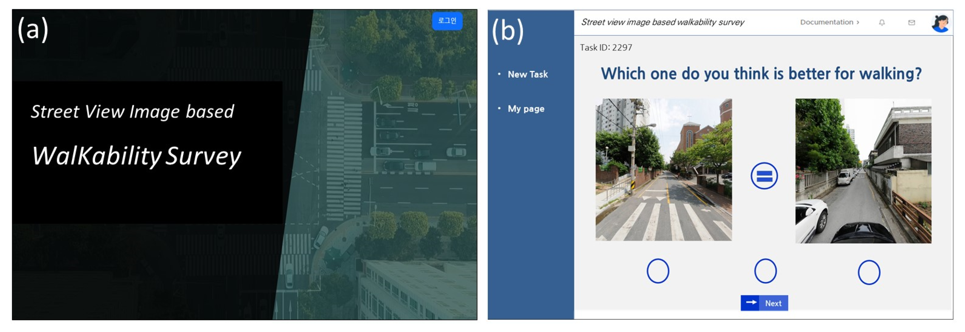
  • Step 2: construct 127,317 pairwise comparisons using crowdsourced data that ask which image was better to walk using 20% of the collected SVIs.
  • Step 3: develop a deep learning model to predict the score of perceived walkability using the training dataset.
  • Step 4: develop an index for evaluating the physical walkability.
  • Step 5: generate the score of the comprehensive physical walkability after constructing data for each indicator by using the semantic segmentation values of SVIs and GIS data.
  • Step 6: visualize a score of the perceived and physical walkability by street, analyze the differences, and then propose alternatives to improve the walkability.

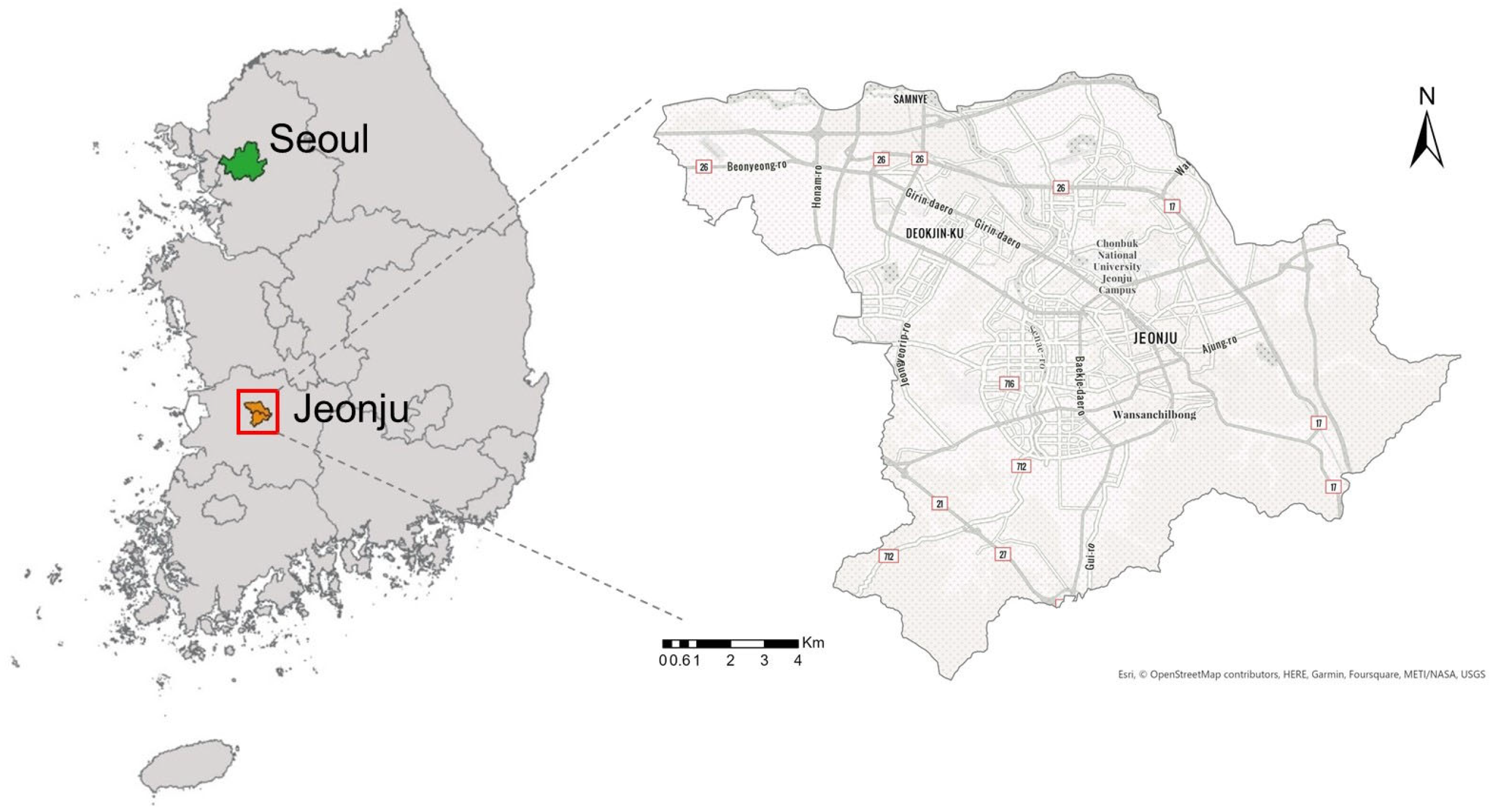
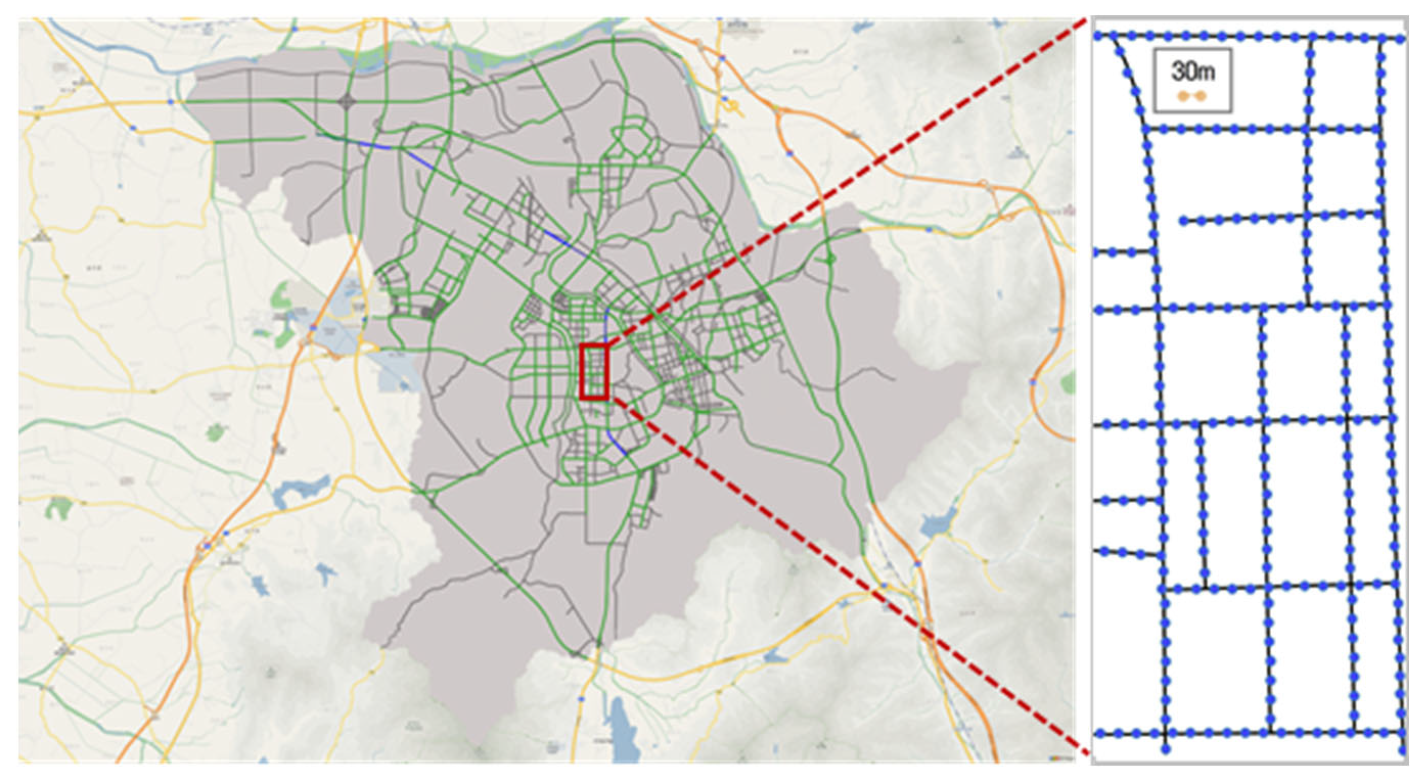
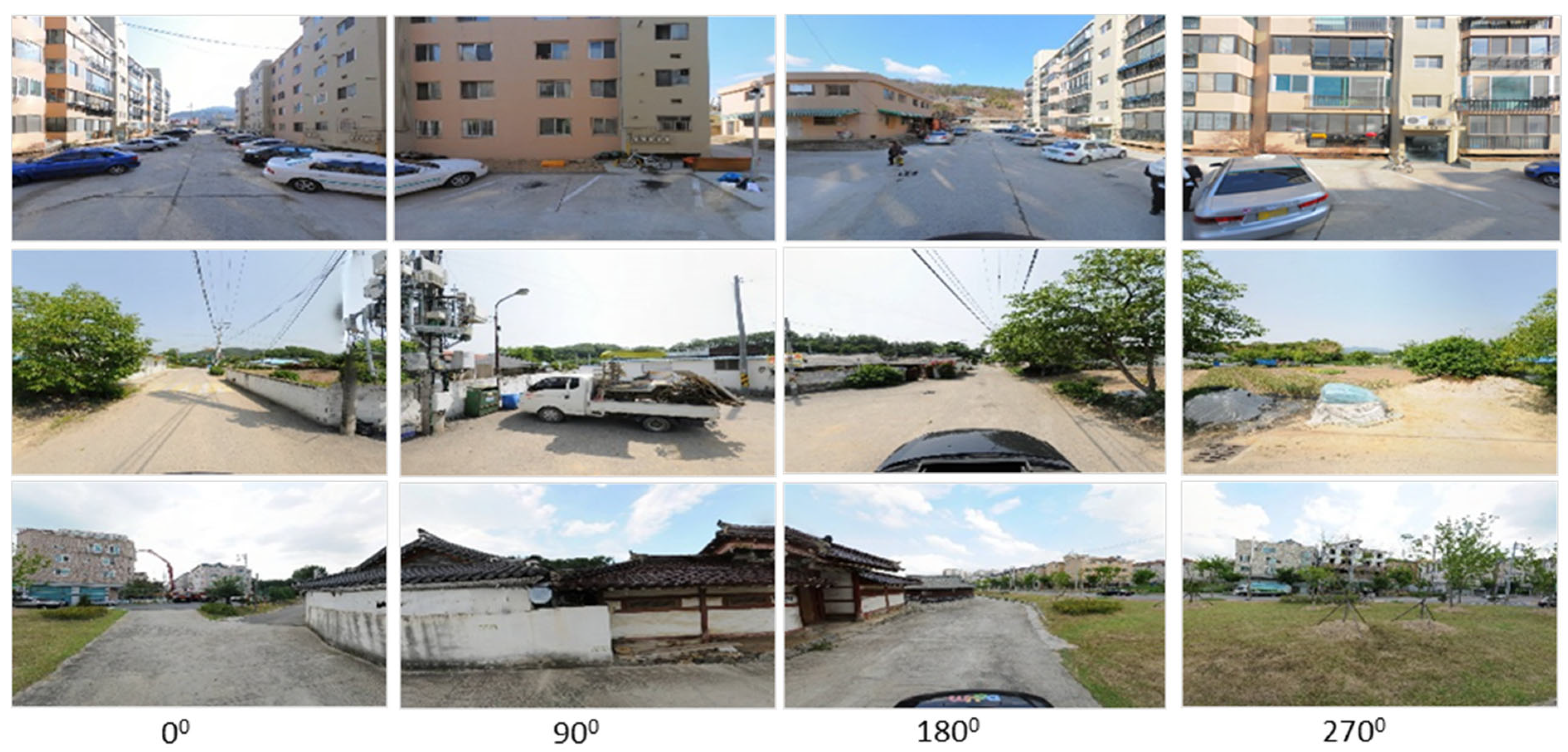
3.1. Collecting SVI Data

In Korea, SVIs can be collected through internet portal sites such as Google, Naver, and Kakao. In this study, we crawled SVIs from Kakao because it provided a relatively shorter update cycle and a wider range of SVIs than Google and Naver. To crawl the SVIs, we generated location coordinates at 30 m intervals using the road network as shown in Figure 3, and extracted a total of 49,156 points in Jeonju, where the total length of the road is 1121 km. Since the SVI was taken in 360-degree panoramic format at a point, we collected the image in 4 directions (0, 90, 180, and 270 degrees) at one point because the image viewed from each direction might be different, as shown in Figure 4. Through this, we finally crawled a total of 196,624 SVIs.

3.2. Construction of a Training Data Set for Predicting the Score of Perceived Walkability

In order to train a model that can predict the score of perceived walkability, a training dataset consisting of SVIs and people’s preference labels is required. Two things should be considered when constructing the training data set: First, what percentage of the entire image dataset should be used as a training dataset? The ratio of the training dataset was set to 20% of the total images. That is, 10,590 points, corresponding to about 20% of the 49,156 total points, were set as the training dataset. The 10,590 points were extracted by a stratification approach in consideration of both road type (boulevard, street, and alley) and land use type (industrial, commercial, and business land use and high-rise and general residential areas). Since there were images in 4 directions at one point, a total of 42,360 SVIs were composed of the training dataset. Second, what assessment method should be applied to analyze SVIs? In this study, we applied a pairwise comparison method because it was known to be more efficient and accurate than a method in which participants gave numerical scores to each SVI [45,46]. To this end, we built a website where participants could select which image was good for walking among two images, as shown in Figure 5. The cyclical pair comparison algorithm proposed by Burton (2003) is widely used for constructing pairwise comparison sets of K times or more [54]. In this study, a pairwise comparison data set was constructed using the K-disjoint pair comparison algorithm and the K-chaining comparison algorithm, which complemented the cyclical pair comparison algorithm [55]. In this study, one image was evaluated at least 6 times to generate a stable score. A total of 52 respondents answered the survey from December 2021 to March 2022, and a total of 127,317 responses were collected. Among them, 120,895 responses were used as the training dataset, except for 6422 responses that answered ‘equal to (=)’. As a result, 80 percent of the valid response data was used as training data, and 20 percent was used as test data.

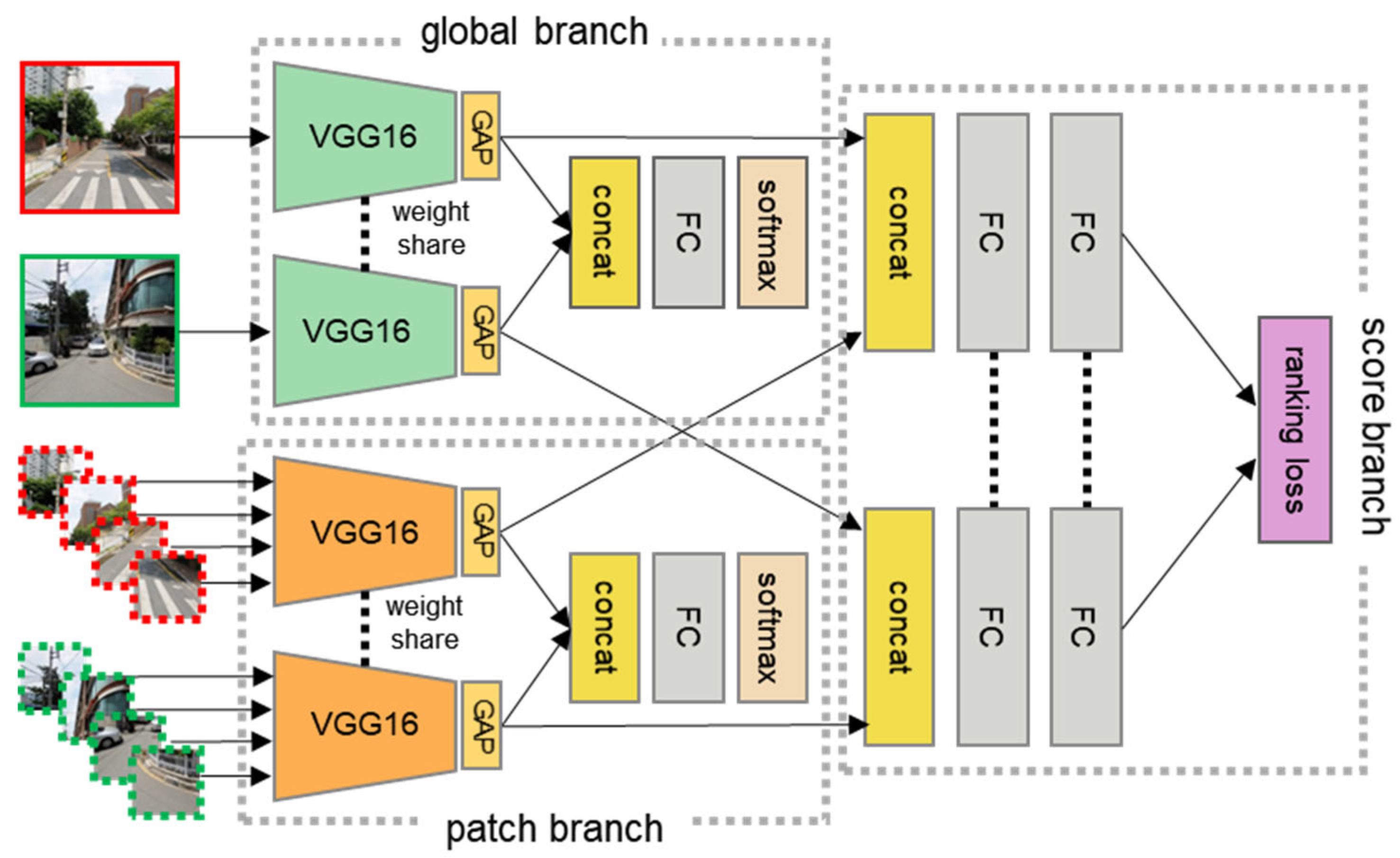
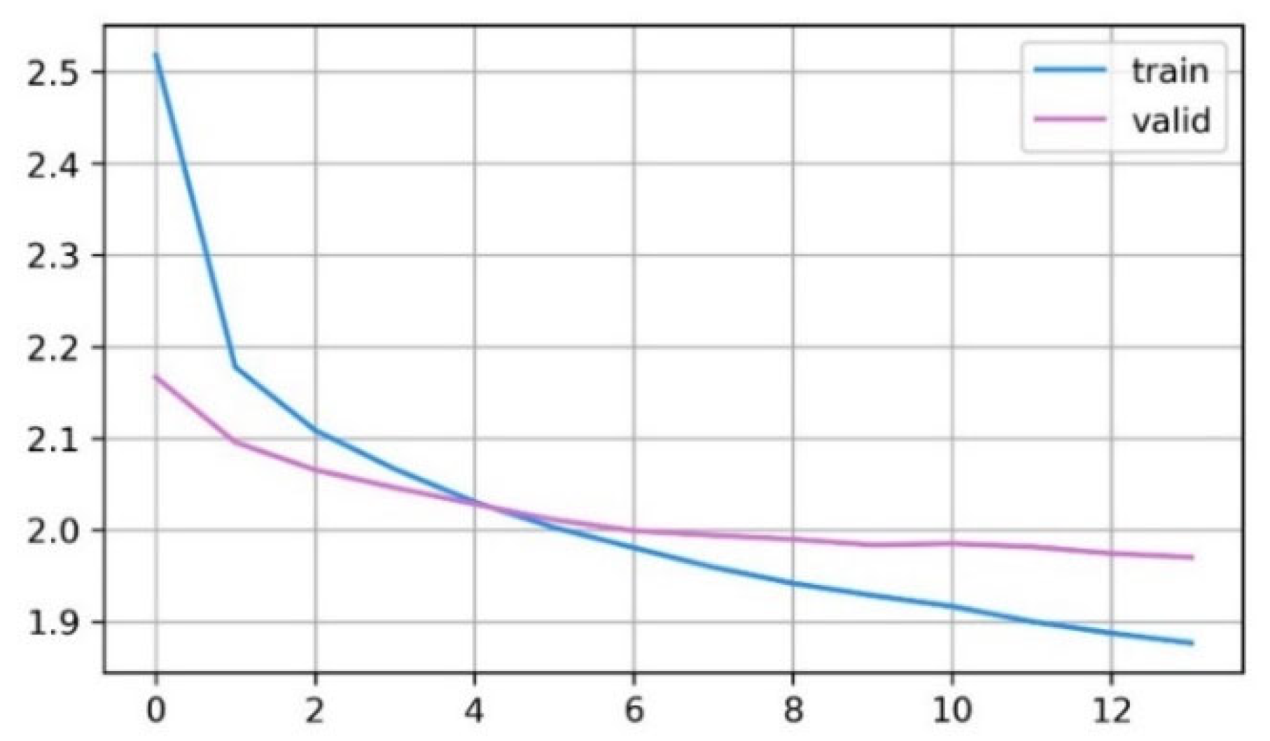
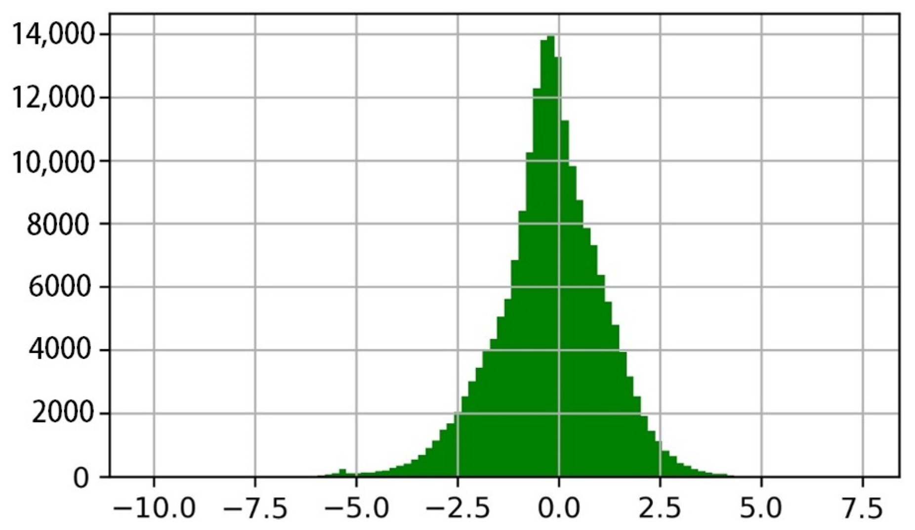
3.3. Development of a Deep Learning Model to Predict Perceived Walkability

For a deep learning model for predicting the score of perceived walkability, the Siamese network and RankNet were set as baseline architectures. In the deep learning model, the Siamese network has a structure in which input images enter in pairs and learn common features of input data, and RankNet has a structure that outputs the final ranking of the pairwise comparison result as a score. That is, the structure of the RSS-CNN model proposed by Dubey et al. [39] was used as a baseline. However, in the case of Jeonju, a medium-sized city, it was necessary to build a structure that could efficiently learn the differences in SVIs even in areas where the differences in the urban landscape were not clear. In consideration of this, we added a structure so that global and regional features appearing in SVIs could be learned together.
The model proposed in this study is composed of three main parts: a patch branch for learning local features, a global branch for learning global features, and a score branch that returns a score by generating a ranking of the SVI based on the previously extracted global and regional features, as shown in Figure 6. The input data is two SVIs that are compared for pairwise comparison, and the final result of the model is the score of the perceived walkability for each image. In the case of the patch branch, four patches generated by cutting one image to a certain size are used as input data in order to learn the local features of the image. Such a multi-patch method is useful when extracting detailed features from an image [56,57,58]. The global branch is responsible for learning the global features of images. Both branches are classified using softmax so that characteristic filters can be learned through comparison between two images. After that, the vector output from each branch is combined for each image, and the RankNet of the score branch is learned along with the superiority values. Based on this, the score of the perceived walkability for each image can be predicted.
The accuracy of the model was calculated using a test dataset consisting of a total of 24,179 pairs. Accuracy was calculated as the matching ratio between the actual and predicted preferences. Four models were designed and evaluated to compare the performance between our model and the models proposed in existing studies. The first baseline model was a model that learned the global features of images and followed the RSS-CNN structure [39]. Considering the number of parameters in the model, the structures of this model were adjusted according to the dataset of this study. The second model was a semantic model proposed by Xu et al. [48] and had a structure to learn the global features of the image and the results of semantic segmentation analysis together. The third model was a patch model that learned only regional patterns that appeared in images and had a structure that removed the global branch part from Figure 6. The fourth model was a global-patch model, which considered both regional and global patterns. All models have experimented under the following three common conditions: the VGG16 model pre-trained on the Places365 dataset was utilized, data augmentation techniques to prevent overfitting and ensure stable learning were applied, and fine tuning was performed only on the top three layers. Table 1 shows the accuracy of the four models for the test dataset, with the global-patch model showing the highest accuracy at 75.01%. This is the result of showing the highest accuracy compared to previous studies that predicted qualitative evaluation through pairwise comparison of images. We confirmed that the global-patch model that learned both global and local features showed higher accuracy than the baseline model that learned only global features or the patch model that learned only regional features. In addition, the patch model that learned regional features was more accurate than the baseline model that learned only global features, indicating that regional features were suitable for improving model performance.
Figure 7 shows the change in the loss value during the training process of the global-patch model, and the model trained up to epoch 8 is used as the final model to prevent overfitting. Figure 8 shows the distribution of the predicted score of perceived walkability for a total of 196,624 SVIs with a global-patch model. It shows the highest number around the mean, −0.21, showing a distribution close to symmetry around the mean value, with a minimum value of −10.21 and a maximum value of 7.52. Figure 9 shows the predicted score of the perceived walkability for the SVIs as an example.

3.4. Development of the Assessment Index of Physical Walkability

To assess the physical walkability, it is necessary to systematize the indicator and build a method. We reviewed studies related to the categories and indicators of walkability and the method of calculating these indicators. In Table 2, the indicators of physical walkability by category were summarized. We derived four categories, such as safety, convenience, comfort, and accessibility, which were the most frequent and considered reasonable. The specific indicators included in each category and their calculation methods varied from researcher to researcher. We reviewed the indicators used in each study for four categories in Table 3. Based on this, we developed a draft of the physical walkability indicators as shown in Table 4.
In Table 4, in the case of SVI data, the accuracy of object segmentation is reviewed, and in the case of GIS data, the data collection and analysis procedures are proposed. To calculate the score for each indicator through the SVIs, the objects that appear in the SVIs are semantically divided using the semantic segmentation model. Semantic segmentation is a deep learning technique that classifies and recognizes images in pixel units by assigning a categorical label to every pixel of the image [61]. In this study, we applied the DeepLab V3 model, among many deep learning models, for semantic segmentation. For image segmentation of SVIs, a training data set that can meaningfully segment SVIs is required. The most representative training data sets include Cityscape and ADE20K [62,63]. The Cityscape divides objects into 30 classes, and ADE20K divides indoor and outdoor images into 150 classes. In this study, object classification was based on ADE20K. Figure 10 shows a semantic segmentation result as an example. There were a total of 12 objects that required accuracy confirmation in the SVI for the evaluation of physical walkability. There were six objects related to the crowdedness indicator (people, cars, buses, trucks, vans, and bicycles), a fence object (existence of sidewalk fences), two objects related to the sidewalk index (roads, sidewalks), and tree, sky, and trash objects related to greenery, sky openness, and the existence of the trash index, respectively. For example, trash was an important factor that hindered comfort in relation to physical walkability, but as shown in Figure 11, flowerpots or wall leaflets were mistakenly recognized as garbage, or garbage was not recognized even when it was present. The accuracy of the semantic segmentation result was confirmed for 40 SVIs drawn from 10 points in consideration of regional characteristics according to land use type, such as residential, commercial, industrial, and agricultural areas in Jeonju. We checked accuracy based on the confusion matrix. For trash objects, the overall accuracy was 87.5%, which was calculated by the equation in Table 5: (TP + TN)/(TP + FP = FN + TN) = (2 + 33)/40. Table 6 shows the accuracy of 12 objects. The accuracy of objects such as the sky, trees, cars, buses, vans, and bicycles was high, but it was relatively low for people and trash objects.
Accuracy = TP + TN/TP + TN + FP + FN
The fence that separates sidewalks and roads is an important factor for pedestrian safety. However, the fence that separated sidewalks and roads, the security window of the building, the fence that divided the center of the roads, etc. were recognized as fences. Therefore, it was judged that additional processing was necessary so that only the fence that separated sidewalks and roads could be classified as a sidewalk fence, as shown in Figure 12. Since the sidewalk fence had the characteristic of being connected to roads or sidewalks, only fences with a road and a sidewalk within a certain distance were classified as sidewalk fences. The SVIs used in this study were 1200 × 1200 pixels, and we created a square filter of 40 pixels in width and length around pixels classified as 32, which was an index of the fence label. The filter was moved one space from the first pixel classified as 32 in the image, and if there were both road and sidewalk indexes 6 and 11 in the filter, we classified the fence as a sidewalk fence, as shown in Figure 13.
In Table 4, the indicators using GIS data were traffic, slope, accessibility to POIs, and distance to public transportation. Areas where traffic accidents frequently occur needed to be reflected in the evaluation of physical walkability. However, the use of the traffic accident data was limited in this study because the data could only be obtained at the mesoscale. In the case of the slope, it was generally calculated using DEM data. Accessibility to POIs was calculated by the distance from the SVI acquisition point to major POIs by crawling the data of 15 types of POIs provided by the Kakao Platform. Accessibility to public transportation was calculated by calculating the distance to the bus stop because Jeonju had no subway as a public transportation option. Table 7 shows the final 8 indicators in consideration of the accuracy of semantic segmentation of SVIs and the possibility of GIS data acquisition.

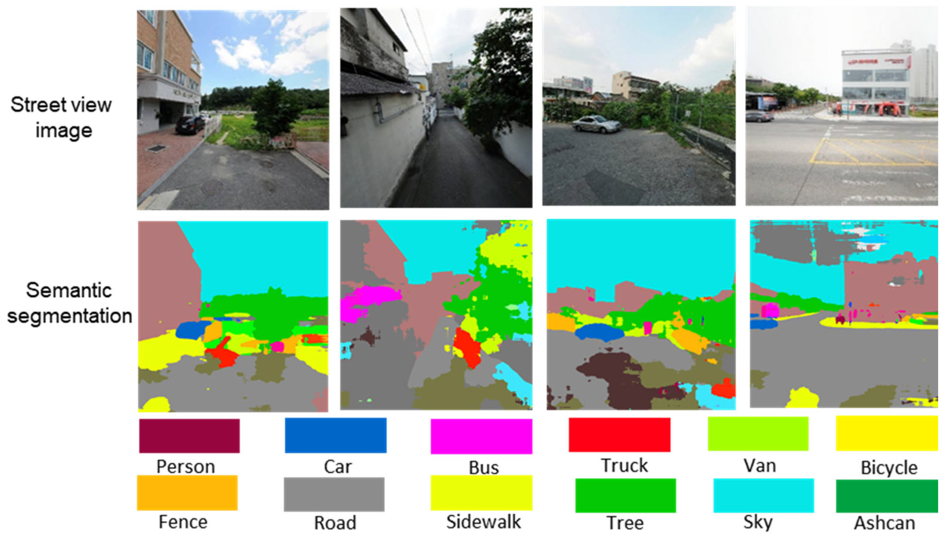
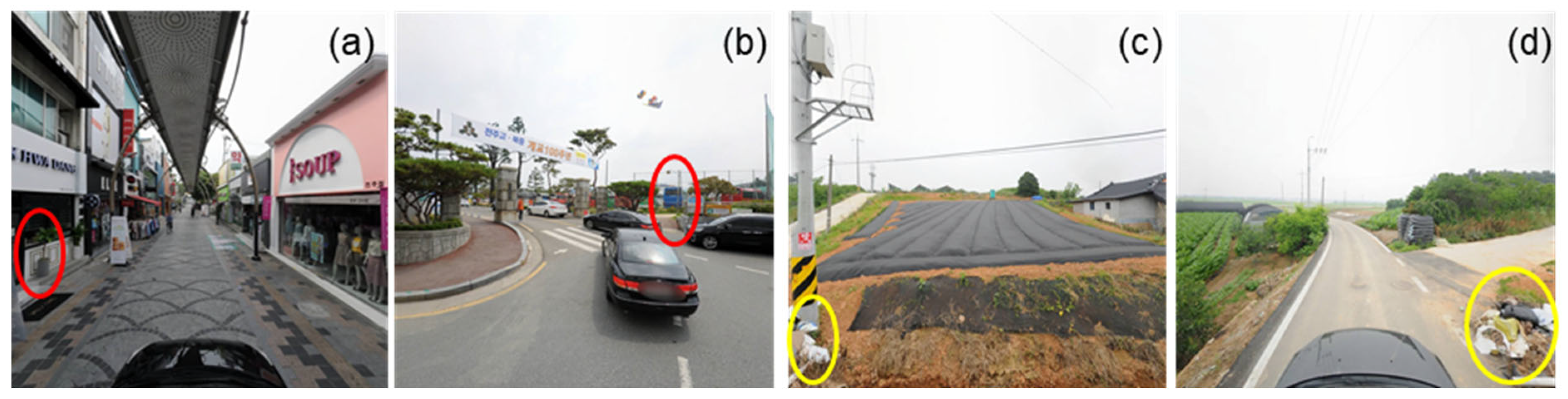
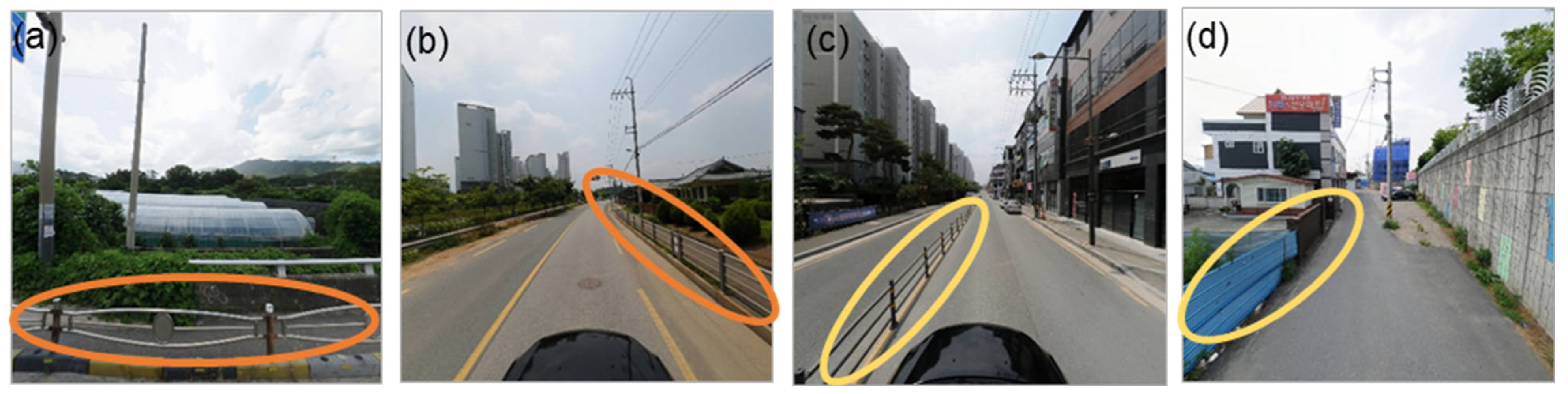
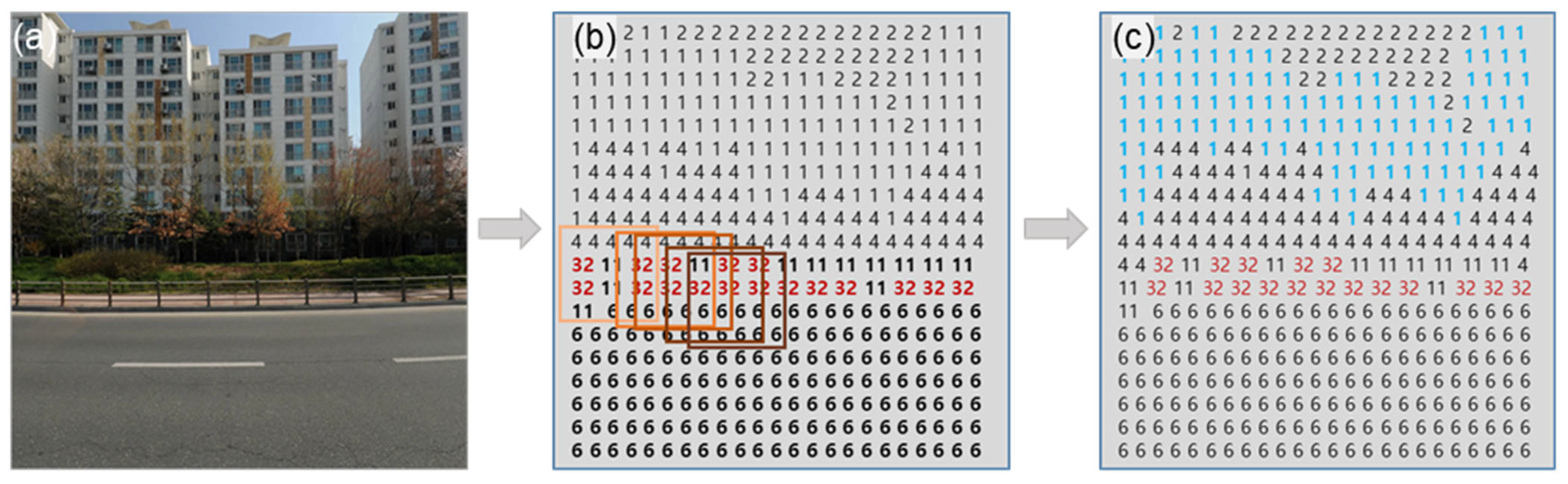
3.5. Database Construction for Physical Walkability Indicators

We constructed the data for the final indicators of physical walkability. When the data source was SVIs, we constructed data with 196,624 images and generated a score for each point by averaging four directions. When the data source was GIS, we generated a score of 49,156 points. A score was given on a scale of 1 to 5 for each indicator, and a high score meant a good physical walking environment. Table 7 summarizes the methods of data construction for each indicator, and Figure 14 is the result of evaluating the scores for eight indicators.
The characteristics of the 8 indicators were as follows: (1) crowdedness was high in the city center and low in the suburbs; (2) sidewalk fence was poor except for some areas in the city center; (3) sidewalk ratio was high in the city center and low in the outskirts, similar to the distribution of residential areas; (4) slope showed a gentle slope in all regions; (5) greenery was high along some boulevard sides, but overall scores were low in both the city center and the outskirts; (6) sky openness was good in the outskirts, but the feeling of openness of the sky in the city center was poor; (7) accessibility to POI was good in the city center and new residential areas; and (8) distance to the bus stop was good in the downtown area and along the roadside.

4. Results

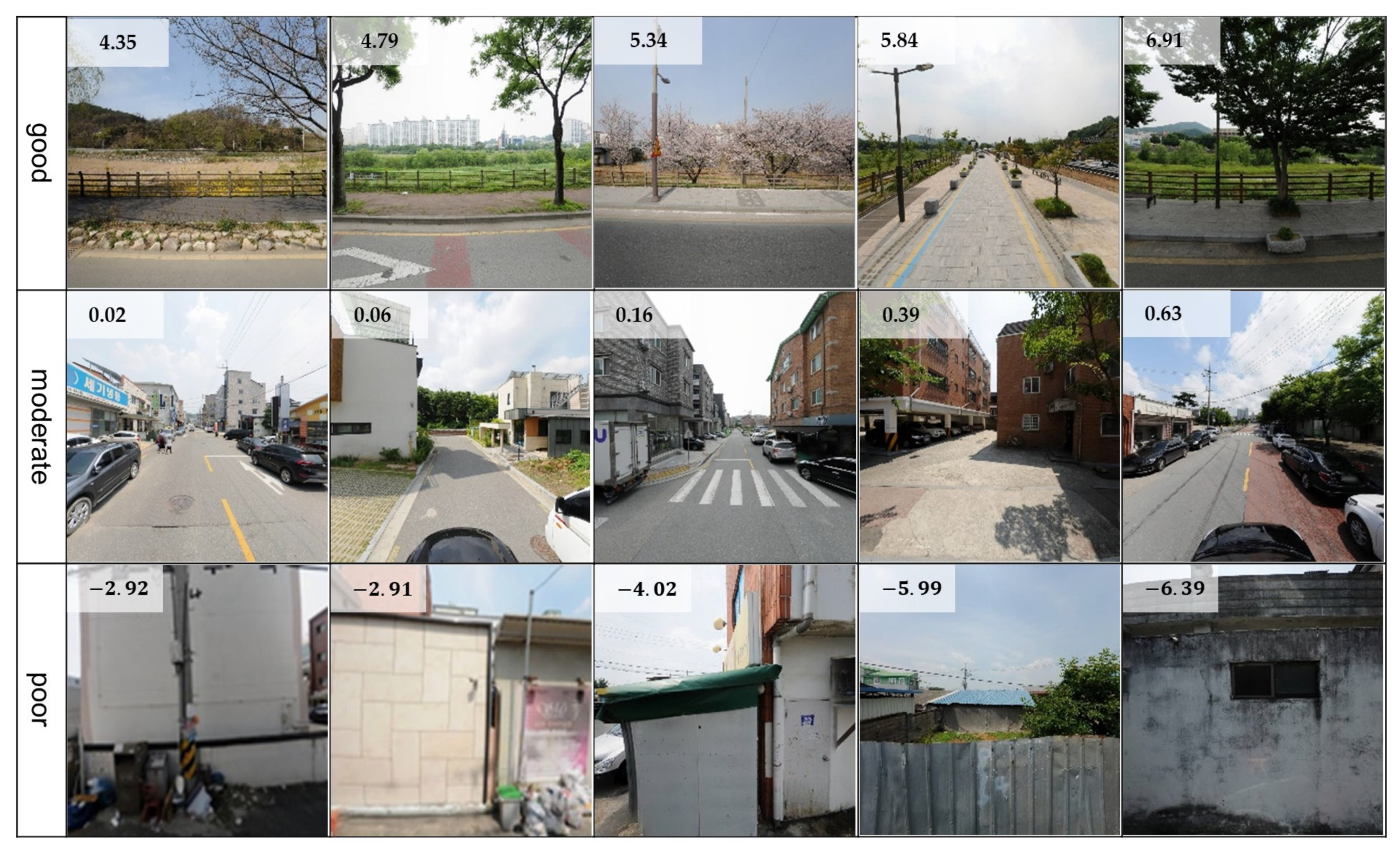
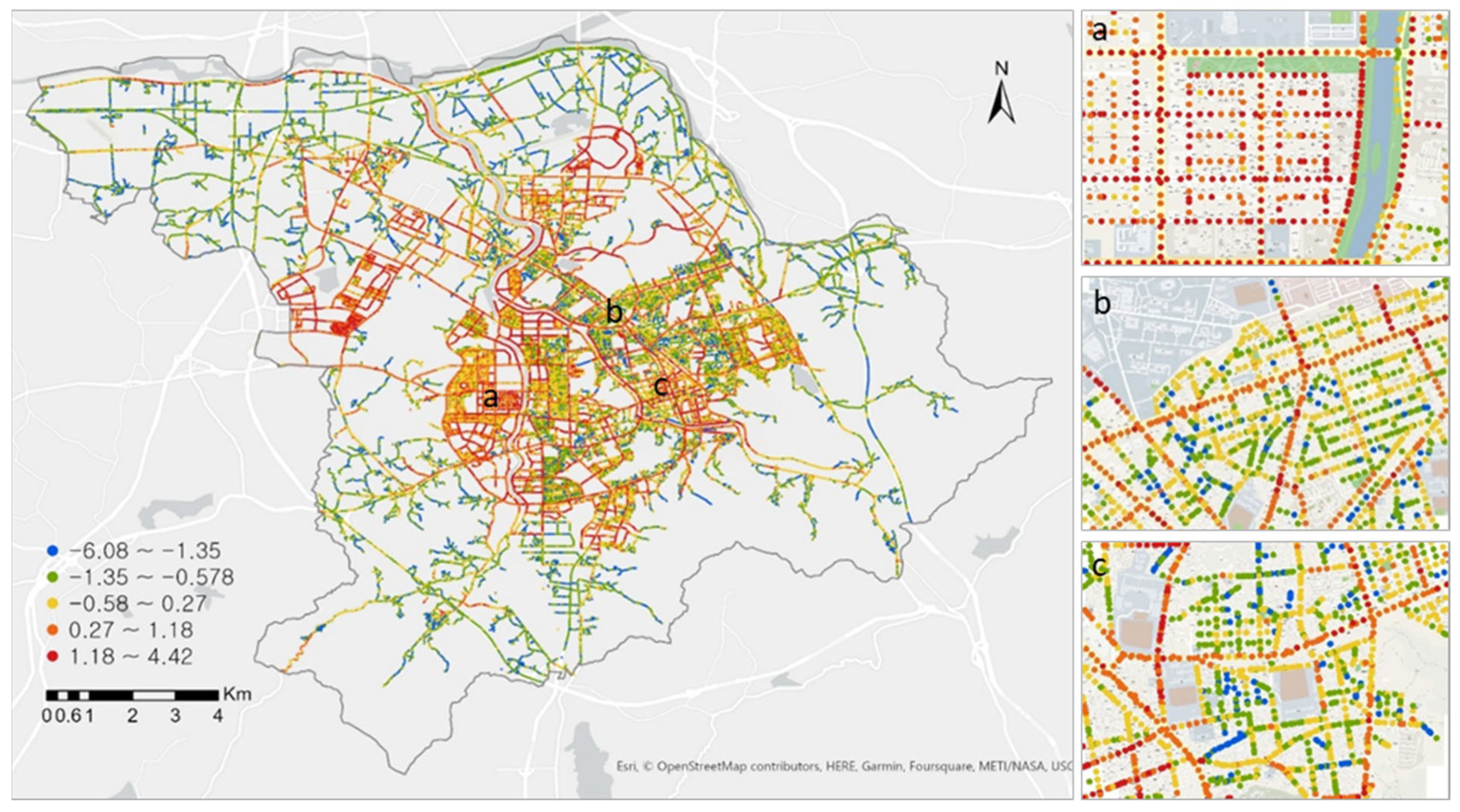
4.1. Visualization of Perceived Walkability

Figure 15 shows the results of visualizing the score of perceived walkability. We calculated the score at one point by averaging the score of four direction images and then divided it into five classes through a natural break. The perceived walkability was relatively good in the city center and new town area, while it was poor on the outskirts of the city. Even within the center of the city, the score of perceived walkability was found to be good in the new town developed as housing complexes, tourist attractions, and boulevards of old town areas. On the other hand, the score of perceived walkability was low even in the center of the city along the back road away from the main road and the old town residential area.

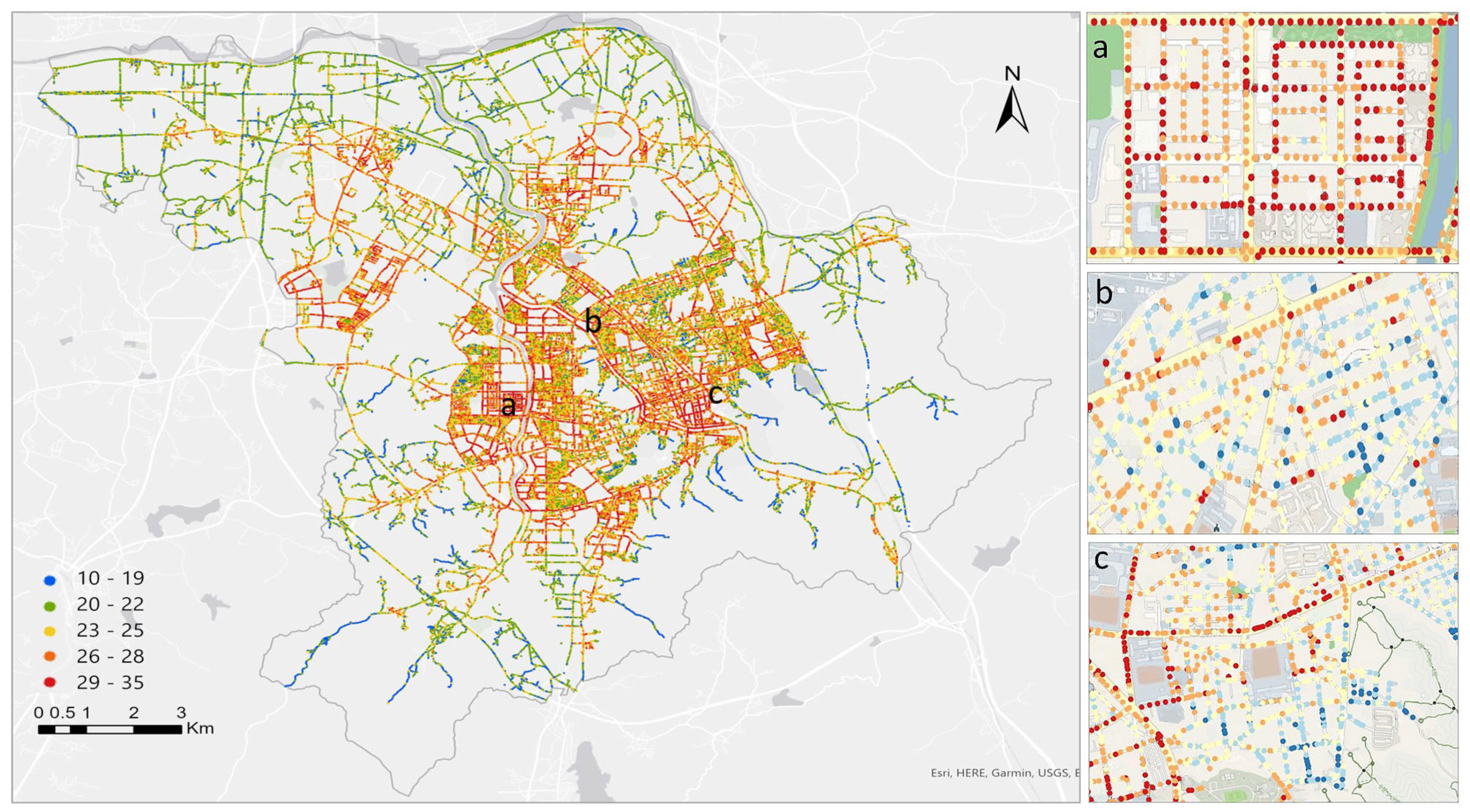
4.2. Visualization of Physical Walkability

The score of physical walkability was calculated by summing the scores of eight indicators. As a result of the combined score, the minimum and maximum scores were 10 and 35, respectively, and the score was divided into five classes by natural break, as shown in Figure 16. In Jeonju, the physical walkability was good in the central area, and, in particular, it was the best around newly constructed large-scale apartment complexes and tourist attractions such as Jeonju Hanok Village. On the other hand, the physical walkability was not good in the outskirts, where the mountain areas were distributed and the rural characteristics were strong. Furthermore, the physical walkability was found to be relatively poor in (1) the outer area with low access to neighborhood facilities or public transportation, (2) the area around factories in industrial complexes, (3) the area where low-rise and row houses were distributed, and (4) the old downtown area where commercial facilities and government offices were concentrated.

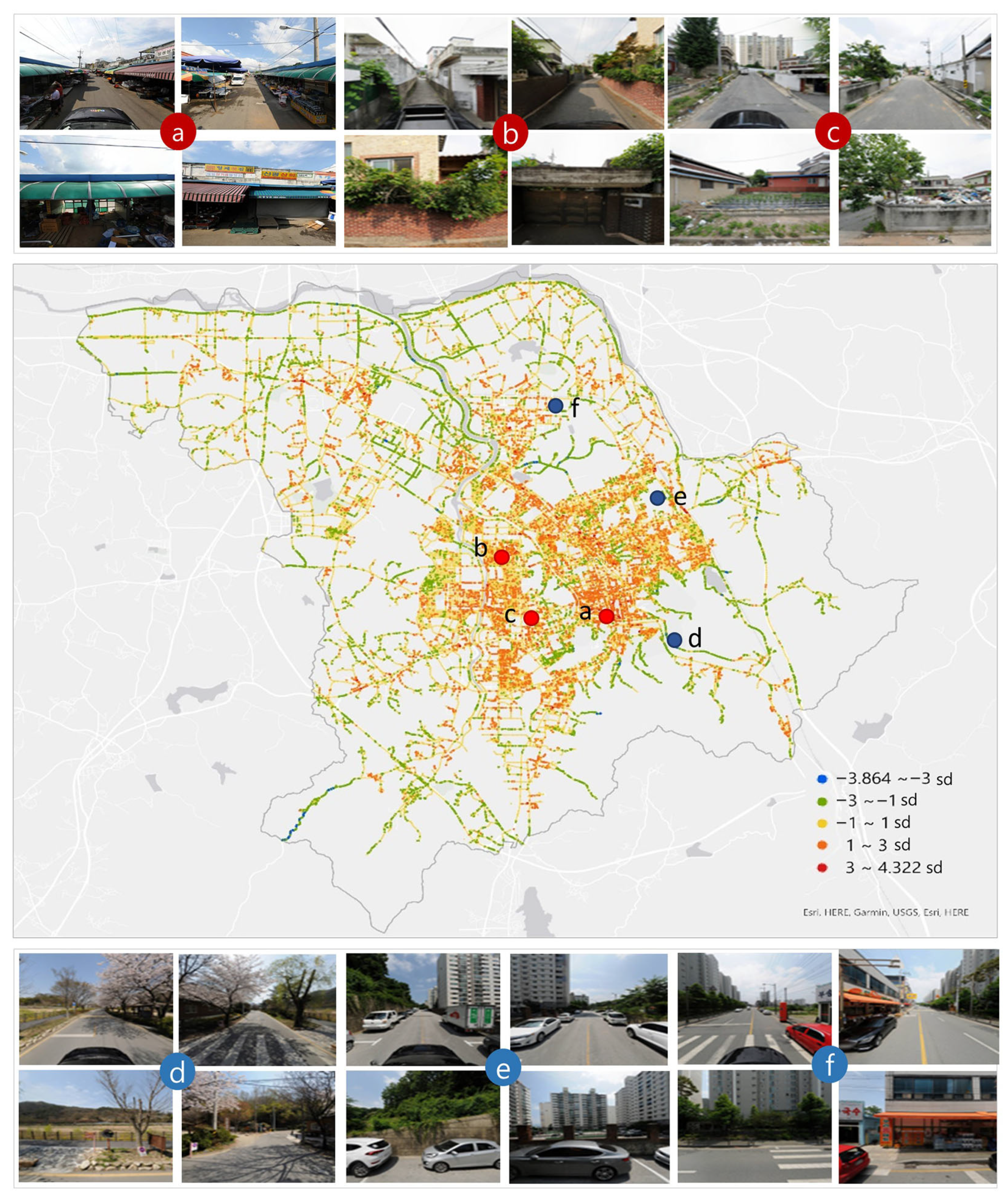
4.3. Difference between Perceived and Physical Walkability

The score of physical walkability showed a distribution between 10 and 35, while the score of perceived walkability had a distribution between −6.8 and 4.4. For a comparison between the physical and perceived walkability, we applied the min–max scaling method by converting the scores into values between zero and one. Then we calculated the difference by subtracting the score of perceived walkability from the one of physical walkability. Figure 17 shows the results of mapping in five classes after finding the standard deviation of the difference values. Areas with positive values were those where the score of physical walkability was higher than the one of perceived walkability, and areas with negative values were the opposite. In Figure 17, the areas marked with red or orange, which appeared mainly in the center of the city, had a higher score of physical walkability than perceived walkability. In particular, the score of physical walkability was much higher than the score of perceived walkability in apartments and housing complexes around Jeonju Express Terminal because the accessibility to neighborhood facilities and the distance to bus stops were good. The area marked in blue or green, which appeared on the outskirts of the city, was the area with a relatively high score of perceived walkability compared to the score of physical walkability, but regions with high scores of perceived walkability appeared discontinuously and intermittently in the center of the city as well. The score of perceived walkability was relatively high in places such as well-maintained areas around large apartment complexes and areas with less accessible but beautiful pedestrian scenery.
The difference between the scores of physical and perceived walkability provided implications for improving the walking environment. In other words, considering the scores of physical and perceived walkability, the areas with high scores of physical walkability but relatively low scores of perceived walkability were judged to be where the walking environment should be improved in priority. Most of these areas appeared in the center of the city. The score of physical walkability was high due to good accessibility indicators, but the score of perceived walkability was relatively low. The area marked in red in Figure 17 was a representative example, and it was necessary to improve the walking environment.

5. Conclusions and Discussion

This study focused on visualizing perceived and physical walkability using SVIs and deep learning technology and analyzing the differences between them. The study area was Jeonju City, one of the medium-sized cities in Korea. 196,624 SVIs were crawled at 30-meter intervals along the road network, and 127,317 pairs of training datasets were constructed by pairwise comparison of about 42,360 SVIs, corresponding to 20% of the acquisition points. After developing a convolutional neural network model that combines the Siamese network and RankNet with global and local patches using the training dataset, the scores of perceived walkability for all collected SVIs were predicted. For the evaluation of physical walkability, eight indicators such as crowdedness, sidewalk fence, sidewalk ratio, slope, greenery, sky openness, accessibility to POIs, and distance to bus stops were selected in a review of existing studies, the accuracy of object classification using the semantic segmentation model, the availability of data acquisition, and redundancy between indicators. Then the score of overall physical walkability was calculated by combining the scores of eight indicators. After that, the scores of perceived and physical walkability were visualized, and the difference between them was analyzed.
The score of physical walkability was almost identically high in the center of the city due to accessibility to neighborhood facilities and distance to bus stops, whereas the score of perceived walkability was high in the center of the city and low in the back streets of the old town, alleys in residential areas, and row houses in the center of the city. The results of assessing perceived and physical walkability provided implications for improving the walking environment. In particular, considering the scores of physical and perceived walkability, the area with a high score of physical walkability but a relatively low score of perceived walkability was judged to be the area where the walking environment should be improved in priority. Most of these areas appeared in the center of the city, especially in the back roads of the old town, row houses, and multi-family clusters.
This study presents novel contributions in three aspects. Firstly, a deep learning model was developed to improve the accuracy of perceived walkability assessments using SVIs, even in small and medium-sized cities where the built environment is less diverse. The basic architecture of the Siamese network and ranking function was applied, and an architecture was added to learn the global and regional features of SVIs so that even small differences in SVIs could be learned effectively. The developed model achieved higher accuracy compared to existing models. Additionally, we built a pairwise comparison dataset for people’s preferred walking environments and made it publicly available on the Figshare platform (https://figshare.com/s/7e0b212bd046e0800f48 (accessed on 23 October 2022)). Secondly, the characteristics of SVIs were analyzed to identify the possibilities and limitations of the semantic segmentation technique. In previous studies, the classification accuracy of objects included in the assessment of physical walkability was not evaluated after applying the semantic segmentation technique. However, in this study, a more sophisticated approach was taken by excluding objects such as trash and people due to their low accuracy and diversifying object processing methods. This indicates the need to develop methodologies suitable for the characteristics of the area when assessing the walking environment in other regions. Thirdly, the differences between perceived and physical walkability were analyzed in detail at the street level, and potential alternatives for improving the walking environment were presented based on the study results. This study provides valuable insights for urban planners and policymakers in understanding the factors that influence perceived and physical walkability, which can ultimately help improve the quality of urban environments.
However, further studies are needed in the future. Although we successfully predicted the perceived walkability score using a deep learning model based on the pairwise comparison dataset, we could not fully understand the factors that influence perceived walkability scores. Investigating the underlying factors that affect perceived walkability is crucial, not only in the domain of walkability research but also in other fields that employ deep learning techniques. The area of explainable AI has gained significant attention in the field of deep learning and can aid in this pursuit. In this study, we employed a semantic segmentation model to identify objects that affect physical walkability. However, we believe that combining semantic segmentation with object detection models can lead to more meaningful assessments. For example, detecting garbage and graffiti can be important factors affecting the comfort of walking, and an object detection model may be more effective in identifying them. Additionally, evaluating walkability during the night is just as important as during the day. Brightness and floating population data may be relevant factors to consider in this regard. Since SVIs capture data at a specific point in time, seasonal variations and changes over time should also be monitored to obtain a comprehensive understanding of walkability.

Author Contributions

Conceptualization, Youngok Kang; methodology, software, validation, and formal analysis, Jiyeon Kim, Jiyoung Park and Jiyoon Lee; data curation, Youngok Kang, Jiyeon Kim and Jiyoung Park; writing—original draft preparation, Youngok Kang; writing—review & editing, Youngok Kang; visualization, Jiyeon Kim and Jiyoung Park; supervision, Youngok Kang; project administration, Youngok Kang; funding acquisition, Youngok Kang. All authors have read and agreed to the published version of the manuscript.

Funding

This research was supported by the Korea Agency for Infrastructure Technology Advancement (KAIA) and funded by the Ministry of Land, Infrastructure, and Transport of the Korean government (Grant No. RS-2022-00143782).

Data Availability Statement

The data and code for the method that supports the findings of this study are available with the identifier at the following link: https://figshare.com/s/7e0b212bd046e0800f48 (accessed on 23 October 2022).

Conflicts of Interest

The authors declare no conflict of interest.

References

  1. Saelens, B.E.; Handy, S.L. Built environment correlates of walking: A review. Med. Sci. Sports Exerc. 2008, 40, 550–566. [Google Scholar] [CrossRef] [PubMed]
  2. Giles-Corti, B.; Kelty, S.F.; Zubrick, S.R.; Villanueva, K.P. Encouraging walking for transport and physical activity in children and adolescents: How important is the built environment? Sports Med. 2009, 39, 995–1009. [Google Scholar] [CrossRef] [PubMed]
  3. Ding, D.; Sallis, J.F.; Kerr, J.; Lee, S.; Rosenberg, D.E. Neighborhood environment and physical activity among youth: A review. Am. J. Prev. Med. 2011, 41, 442–455. [Google Scholar] [CrossRef] [PubMed]
  4. Leslie, E.; Coffee, N.; Frank, L.; Owen, N.; Bauman, A.; Hugo, G. Walkability of local communities: Using geographic information systems to objectively assess relevant environmental attributes. Health Place 2007, 13, 111–122. [Google Scholar] [CrossRef] [PubMed]
  5. Rogers, S.H.; Halstead, J.M.; Gardner, K.H.; Carlson, C.H. Examining walkability and social capital as indicators of quality of life at the municipal and neighborhood scales. Appl. Res. Qual. Life 2011, 6, 201–213. [Google Scholar] [CrossRef]
  6. Cortright, J. Walking the Walk: How Walkability Raises Home Values in U.S. Cities. Chicago, Illinois, USA, CEOs for Cities. 2009. Available online: http://www.ceosforcities.org/pagefiles/WalkingTheWalk_CEOsforCities.pdf (accessed on 5 October 2022).
  7. Pivo, G.; Fisher, J.D. The walkability premium in commercial real estate investments. Real Estate Econ. 2011, 39, 185–219. [Google Scholar] [CrossRef]
  8. Marshall, J.D.; Brauer, M.; Frank, L.D. Healthy neighborhoods: Walkability and air pollution. Environ. Health Perspect. 2009, 117, 1752–1759. [Google Scholar] [CrossRef]
  9. Fonseca, F.; Ribeiro, P.J.; Conticelli, E.; Jabbari, M.; Papageorgiou, G.; Tondelli, S.; Ramos, R.A. Built environment attributes and their influence on walkability. Int. J. Sustain. Transp. 2022, 16, 660–679. [Google Scholar] [CrossRef]
  10. Transport for London. London Travel Report 2005. 2005. Available online: http://content.tfl.gov.uk/london-travel-report-2005.pdf (accessed on 12 November 2022).
  11. WHO Regional Office for Europe. The European Health Report 2009: Health and Health Systems. 2009. Available online: http://www.euro.who.int/__data/assets/pdf_file/0009/82386/E93103.pdf (accessed on 24 November 2022).
  12. Toronto Public Health. The Walkable City: Neighborhood Design and Preferences, Travel Choices and Health (A Healthy Toronto by Design Report). 2012. Available online: http://www.toronto.ca/health/hphe/pdf/walkable_city.pdf (accessed on 8 April 2022).
  13. Giles-Corti, B.; Vernez-Moudon, A.; Reis, R.; Turrell, G.; Dannenberg, A.L.; Badland, H.; Foster, S.; Lowe, M.; Sallis, J.F.; Stevenson, M.; et al. City planning and population health: A global challenge. Lancet 2016, 388, 2912–2924. [Google Scholar] [CrossRef]
  14. Ministry of Public Administration and Security of Korea. Act on the Promotion of Pedestrian Safety and Convenience Enhancement Act; Ministry of Public Administration and Security of Korea: Seoul, Republic of Korea, 2012.
  15. Cervero, R.; Kockelman, K. Travel demand and the 3Ds: Density, diversity, and design. Transp. Res. Part D Transp. Environ. 1997, 2, 199–219. [Google Scholar] [CrossRef]
  16. Saelens, B.E.; Sallis, J.F.; Frank, L.D. Environmental correlates of walking and cycling: Findings from the transportation, urban design, and planning literatures. Ann. Behav. Med. 2003, 25, 80–91. [Google Scholar] [CrossRef] [PubMed]
  17. Rodríguez, D.A.; Evenson, K.R.; Roux, A.V.D.; Brines, S.J. Land use, residential density, and walking. Am. J. Prev. Med. 2009, 37, 397–404. [Google Scholar] [CrossRef]
  18. Ewing, R.; Cervero, R. Travel and the Built Environment. J. Am. Plann. Assoc. 2010, 76, 265–294. [Google Scholar] [CrossRef]
  19. Wang, W.; Li, P.; Wang, W.; Namgung, M. Exploring determinants of pedestrians’ satisfaction with sidewalk environments: Case study in Korea. J. Urban Plan. Dev. 2012, 138, 166–172. [Google Scholar] [CrossRef]
  20. Mateo-Babiano, I. Pedestrian’s needs matter: Examining Manila’s walking environment. Transp. Policy 2016, 45, 107–115. [Google Scholar] [CrossRef]
  21. Lee, E.; Dean, J. Perceptions of walkability and determinants of walking behavior among urban seniors in Toronto, Canada. J. Transp. Health 2018, 9, 309–320. [Google Scholar] [CrossRef]
  22. Arellana, J.; Saltarín, M.; Larrañaga, A.M.; Alvarez, V.; Henao, C.A. Urban walkability considering pedestrians’ perceptions of the built environment: A 10-year review and a case study in a medium-sized city in Latin America. Transp. Rev. 2020, 40, 183–203. [Google Scholar] [CrossRef]
  23. Kim, K.; Lee, J. Pedestrian Cognition and Satisfaction on the Physical Elements in Pedestrian Space. J. Urban Des. Inst. Korea 2016, 17, 89–103. [Google Scholar]
  24. Chiang, Y.C.; Sullivan, W.; Larsen, L. Measuring neighborhood walkable environments: A comparison of three approaches. Int. J. Environ. Res. Public Health 2017, 14, 593. [Google Scholar] [CrossRef]
  25. Frank, L.D.; Schmid, T.L.; Salis, J.F.; Chapman, J.; Saelems, B.E. Linking Objectively Measured Physical Activity with Objectively Measured Urban Form: Findings from SMARTRAQ. Am. J. Prev. Med. 2005, 28, 117–125. [Google Scholar] [CrossRef]
  26. Lee, K.; Ahn, K. An Empirical Analysis of Neighborhood Environment Affecting Residents’ Walking: Case study of 12 Areas in Seoul. J. Archit. Ins. Korea Plan. Des. 2008, 24, 293–302. [Google Scholar]
  27. Lee, C.; Moudon, A.V. The 3Ds + R: Quantifying Land Use and Urban Form Correlates of Walking. Transp. Res. Part D Transp. Environ. 2006, 11, 204–215. [Google Scholar] [CrossRef]
  28. Weiss, R.L.; Maantay, J.A.; Fahs, M. Promoting active urban aging: A measurement approach to neighborhood walkability for older adults. Cities Environ. 2010, 3, 12. [Google Scholar] [CrossRef]
  29. Kim, S.; Park, S.; Lee, J.S. Meso-or micro-scale? Environmental factors influencing pedestrian satisfaction. Transp. Res. Part D Transp. Environ. 2014, 30, 10–20. [Google Scholar] [CrossRef]
  30. Quercia, D.; Aiello, L.M.; Schifanella, R.; Davies, A. The digital life of walkable streets. In Proceedings of the 24th International Conference on World Wide Web, Florence, Italy, 18–22 May 2015; pp. 875–884. [Google Scholar]
  31. Zhou, H.; He, S.; Cai, Y.; Wang, M.; Su, S. Social inequalities in neighborhood visual walkability: Using street view imagery and deep learning technologies to facilitate healthy city planning. Sustain. Cities Soc. 2019, 50, 101605. [Google Scholar] [CrossRef]
  32. Li, Y.; Yabuki, N.; Fukuda, T.; Zhang, J. A big data evaluation of urban street walkability using deep learning and environmental sensors-a case study around Osaka University Suita campus. In Proceedings of the 38th eCAADe Conference, Berlin, Germany, 16–18 September 2020; pp. 319–328. [Google Scholar]
  33. Wu, C.; Peng, N.; Ma, X.; Li, S.; Rao, J. Assessing multiscale visual appearance characteristics of neighborhoods using geographically weighted principal component analysis in Shenzhen, China. Comput. Environ. Urban Syst. 2020, 84, 101547. [Google Scholar] [CrossRef]
  34. Li, X.; Ratti, C. Mapping the spatial distribution of shade provision of street trees in Boston using Google Street View panoramas. Urban For. Urban Gree 2018, 31, 109–119. [Google Scholar] [CrossRef]
  35. Humpel, N.; Owen, N.; Leslie, E.; Marshall, A.L.; Bauman, A.E.; Sallis, J.F. Associations of location and perceived environmental attributes with walking in neighborhoods. Am. J. Health Promot. 2004, 18, 239–242. [Google Scholar] [CrossRef]
  36. Park, S.; Choi, Y.; Seo, H.; Kim, J. Perception of Pedestrian Environment and Satisfaction of Neighborhood Walking—An Impact Study based on Four Residential Communities in Seoul, Korea. J. Archit. Ins. Korea Plan. Des. 2009, 25, 253–261. [Google Scholar]
  37. Vallejo-Borda, J.A.; Cantillo, V.; Rodriguez-Valencia, A. A perception-based cognitive map of the pedestrian perceived quality of service on urban sidewalks. Transp. Res. Part F Traffic Psychol. Behav. 2020, 73, 107–118. [Google Scholar] [CrossRef]
  38. Salesses, P.; Schechtner, K.; Hidalgo, C.A. The Collaborative Image of The City: Mapping the Inequality of Urban Perception. PLoS ONE 2013, 10, e0119352. [Google Scholar] [CrossRef] [PubMed]
  39. Dubey, A.; Naik, N.; Parikh, D.; Raskar, R.; Hidalgo, C.A. Deep learning the city: Quantifying urban perception at a global scale. In Proceedings of the European Conference on Computer Vision, Amsterdam, The Netherlands, 8–16 October 2016; pp. 196–212. [Google Scholar]
  40. Wang, R.; Liu, Y.; Lu, Y.; Zhang, J.; Liu, P.; Yao, Y.; Grekousis, G. Perceptions of built environment and health outcomes for older Chinese in Beijing: A big data approach with street view images and deep learning technique. Comput. Environ. Urban Syst. 2019, 78, 101386. [Google Scholar] [CrossRef]
  41. Biljecki, F.; Ito, K. Street view imagery in urban analytics and GIS: A review. Landsc. Urban Plan. 2021, 215, 104217. [Google Scholar] [CrossRef]
  42. Kim, J.H.; Lee, S.; Hipp, J.R.; Ki, D. Decoding urban landscapes: Google street view and measurement sensitivity. Comput. Environ. Urban Syst. 2021, 88, 101626. [Google Scholar] [CrossRef]
  43. Blečić, I.; Cecchini, A.; Trunfio, G.A. Towards automatic assessment of perceived walkability. In Proceedings of the International Conference on Computational Science and Its Application, Melbourne, Australia, 2–5 July 2018; pp. 351–365. [Google Scholar]
  44. Santani, D.; Ruiz-Correa, S.; Gatica-Perez, D. Looking south: Learning urban perception in developing cities. ACM Trans. Soc. Comput. 2018, 1, 1–23. [Google Scholar] [CrossRef]
  45. Bijmolt, T.H.; Wedel, M. The effects of alternative methods of collecting similarity data for multidimensional scaling. Int. J. Res. Mark. 1995, 124, 363–371. [Google Scholar] [CrossRef]
  46. Stewart, N.; Brown, G.D.; Chater, N. Absolute identification by relative judgment. Psychol. Rev. 2005, 112, 881–911. [Google Scholar] [CrossRef]
  47. Min, W.; Mei, S.; Liu, L.; Wang, Y.; Jiang, S. Multi-task deep relative attribute learning for visual urban perception. IEEE Trans. Image Process. 2019, 29, 657–669. [Google Scholar] [CrossRef]
  48. Xu, Y.; Yang, Q.; Cui, C.; Shi, C.; Song, G.; Han, X.; Yin, Y. Visual Urban Perception with Deep Semantic-Aware Network. In Proceedings of the International Conference on Multimedia Modeling, Thessaloniki, Greece, 8–11 January 2019; pp. 28–40. [Google Scholar]
  49. Guan, W.; Chen, Z.; Feng, F.; Liu, W.; Nie, L. Urban Perception: Sensing Cities via a Deep Interactive Multitask Learning Framework. ACM Trans. Multim. Comput. 2021, 17, 1–20. [Google Scholar] [CrossRef]
  50. Koch, G.; Zemel, R.; Salakhutdinov, R. Siamese Neural Networks for One-Shot Image Recognition. ICML Deep Learning Workshop. 2015, Volume 2. Available online: https://www.cs.toronto.edu/~zemel/documents/oneshot1.pdf (accessed on 5 October 2022).
  51. Koczkodaj, W.W.; Szybowski, J. Pairwise comparisons simplified. Appl. Math. Comput. 2015, 253, 387–394. [Google Scholar] [CrossRef]
  52. Saha, A.; Shivanna, R.; Bhattacharyya, C. How many pairwise preferences do we need to rank a graph consistently? In Proceedings of the AAAI Conference on Artificial Intelligence, Honolulu, HI, USA, 27 January–1 February 2019; Volume 33, pp. 4830–4837. [Google Scholar] [CrossRef]
  53. Sunahase, T.; Baba, Y.; Kashima, H. Pairwise HITS: Quality estimation from pairwise comparisons in creator-evaluator crowdsourcing process. In Proceedings of the AAAI Conference on Artificial Intelligence, San Francisco, CA, USA, 4–9 February 2017; Volume 31, pp. 977–983. [Google Scholar] [CrossRef]
  54. Burton, M.L. Too Many Questions? The Uses of Incomplete Cyclic Designs for Paired Comparisons. Field Methods 2003, 15, 115–130. [Google Scholar] [CrossRef]
  55. Yoo, K.; Lee, D.; Lee, C.; Nam, K. Generating Pairwise Comparison Set for Crowed Sourcing based Deep Learning. J. Korea Ind. Inf. Syst. Res. 2022, 27, 1–11. [Google Scholar] [CrossRef]
  56. Lu, X.; Lin, Z.; Jin, H.; Yang, J.; Wang, J.Z. Rapid: Rating pictorial aesthetics using deep learning. In Proceedings of the 22nd ACM international conference on Multimedia, Orlando, FL, USA, 3–7 November 2014; Volume 3, pp. 457–466. [Google Scholar]
  57. Lu, X.; Lin, Z.; Shen, X.; Mech, R.; Wang, J.Z. Deep multi-patch aggregation network for image style, aesthetics, and quality estimation. In Proceedings of the IEEE International Conference on Computer Vision, Santiago, Chile, 7–13 December 2015; pp. 990–998. [Google Scholar]
  58. Zou, W.; Zhang, D.; Lee, D.J. A new multi-feature fusion based convolutional neural network for facial expression recognition. Appl. Intell. 2021, 52, 2918–2929. [Google Scholar] [CrossRef]
  59. Lee, S.; Ko, J.; Lee, G. An Analysis of Neighborhood Environment Affecting Walking Satisfaction-Focused on the ‘Seoul Survey’ 2013. J. Korea Plan. Assoc. 2016, 51, 169–187. [Google Scholar] [CrossRef]
  60. Park, K.D.; Lee, S.K. Structural Relationship between Neighborhood Environment, Daily Walking Activity, and Subjective Health Status: Application of Path Model. J. Korea Plan. Assoc. 2018, 53, 255–272. [Google Scholar] [CrossRef]
  61. Wang, P.; Chen, P.; Yuan, Y.; Liu, D.; Huang, Z.; Hou, X.; Cottrell, G. Understanding convolution for semantic segmentation. In Proceedings of the 2018 IEEE Winter Conference on Applications of Computer Vision, Lake Tahoe, NV, USA, 12–15 March 2018; pp. 1451–1460. [Google Scholar]
  62. Cityscapes. Available online: https://www.cityscapes-dataset.com (accessed on 2 January 2023).
  63. ADE20K. Available online: https://groups.csail.mit.edu/vision/datasets/ADE20K (accessed on 2 January 2023).
Figure 1. Study area.
Ijgi 12 00186 g001
Figure 2. Research flow.
Ijgi 12 00186 g002
Figure 3. Road network in Jeonju and an example of data collection at a 30 m interval.
Ijgi 12 00186 g003
Figure 4. Example of SVIs: each row represents the same location, and the number indicates the data collection angle of the same point: 0°: front, 90°: right, 180°: back, and 270°: left.
Ijgi 12 00186 g004
Figure 5. Web-based walking environment survey site: (a) landing page, (b) crowdsourcing evaluation page.
Ijgi 12 00186 g005
Figure 6. Deep learning model architecture for perceived walking score prediction.
Ijgi 12 00186 g006
Figure 7. Training loss: the x-axis represents epochs, and the y-axis represents loss values.
Ijgi 12 00186 g007
Figure 8. Distribution of perceived walkability score for 196,624 SVIs: the x-axis represents perceived walkability score, and the y-axis presents the number of SVIs.
Ijgi 12 00186 g008
Figure 9. Examples of the perceived walkability score of SVIs.
Ijgi 12 00186 g009
Figure 10. Example of the result of semantic segmentation.
Ijgi 12 00186 g010
Figure 11. Examples of trash object misclassifications: (a) segmenting flowerpots as trash, (b) segmenting banners as trash, and (c,d) failure to segment trash.
Ijgi 12 00186 g011
Figure 12. Examples of fences that were segmented as a fence: (a,b) a fence that is separating the sidewalk from the road, (c) a fence that is dividing the center of the road, and (d) a fence that is separating the vacant lot.
Ijgi 12 00186 g012
Figure 13. Example of SVI processing to classify sidewalk fences: (a) original image, (b) apply a filter of size 40 × 40 around the pixel with 32 and move the filter along 32, and (c) if there are 6 and 11 in the filter, it is judged as a sidewalk fence. Note: 32, 6, and 11 represent indices of fence, road, and sidewalk, respectively.
Ijgi 12 00186 g013
Figure 14. The scores of physical walkability by the 8 indicators: red dot: 5 pts, orange dot: 4 pts, yellow dot: 3 pts, green dot: 2 pts, and blue dot: 1 pt.
Ijgi 12 00186 g014
Figure 15. Visualization of perceived walkability by street: (a) new town area and (b,c) old town area.
Ijgi 12 00186 g015
Figure 16. Visualization of physical walkability by street: (a) new town area and (b,c) old town area.
Ijgi 12 00186 g016
Figure 17. Difference between the scores of perceived and physical walkability: (ac) areas where the score of physical walkability was higher than the one of perceived walkability; (df) areas where the score of physical walkability was lower than the one of perceived walkability. (a) Traditional market in the old town, (b) multi-family area in the old city center, (c) detached house area in the old city center, (d) area where roads around cultural properties are developed outside the city center, (e) area where new roads and apartments were constructed with the construction of new railroad stations, and (f) new housing development district outside the city.
Ijgi 12 00186 g017
Table 1. Comparison of accuracy between models.
ModelAccuracy
Baseline model (RSS_CNN)73.87%
Semantic model73.64%
Patch model74.62%
Global-Patch model75.01%
Table 2. Physical walkability assessment category.
Zhou et al. [31]Li et al. [32]Blečić et al. [43]Li and Latti [34]Lee et al. [59]Park and Lee [60]Kim et al. [29]Quercia et al. [30]Mateo-Babiano [20]
Safety
Convenience
Comfort● ○
Accessibility
Connectivity
Perceptibility
Conviviality
Diversity
Note: ●: SVIs used, ○: other than SVIs used.
Table 3. Specific indicators by category of physical walkability.
IndicatorsZhou et al. [31]Li et al. [32]Blečić et al. [43]Li and Latti [34]Lee et al. [59]Park and Lee [60]Kim et al. [29]Quercia et al. [30]Mateo-Babiano [20]
SafetyVisual crowdedness
Light
Continuity of the school zone
Crossing
Bus lane
Sidewalk fence
Traffic signal
Street light
Car accident
Crime
CCTV
Police officer at the intersection
ConvenienceVisual pavement
Slope
Width of the sidewalk
Sidewalk width and quality
Continuity of the sidewalk
Signboard
Street facility
ComfortPsychological greenery
Outdoor enclosure
Enclosure
Sky view factor
Pedestrian density
Noise
Density of trees along the street
Ratio of park/green area
Existence of trees
Existence of trash
Existence of shade
Accessi
bility
Accessibility to the POI
Ratio of a 4 lane road
Density of the bus station
Class 1 facility within 500 m
Class 2 facility within 500 m
Complex mall within 500 m
Distance to bus stop
Distance to the subway station
Note: ●: SVIs used, ○: other than SVIs used.
Table 4. Physical walkability indicator (draft).
CategoryIndicatorMethodData Source
SafetyVisual crowdedness Obstacle ( car ,   bicycle ,   truck ,   van ,   person )   pixel / Total   pixel SVI
Existence of a fenceExistence of a sidewalk fenceSVI
ConvenienceSidewalk ratio Sidewalk   pixel / Road   pixel SVI
Slope GIS data (DEM)
ComfortGreenery Tree   pixel / Total   pixel SVI
Sky openness Sky   pixel / Total   pixel SVI
Existence of trashExistence of trashSVI
AccessibilityAccessibility to the POIDistance to POIPOI/GIS data
Distance to public transportationDistance to public transportationGIS data
Table 5. Object classification accuracy (trash).
True ConditionPredicted Condition
PositiveNegative
PositiveTrue Positive (TP): 2False Negative (FN): 2
NegativeFalse Positive (FP): 3True Negative (TN): 33
Table 6. Accuracy of 12 objects required for evaluating physical walkability.
ObjectAccuracy (%)Description
1Sky(40/40) × 100 = 100.0
2Tree(40/40) × 100 = 100.0
3Fence(34/40) × 100 = 85.0Need to extract sidewalk fences between sidewalk and road.
4Sidewalk
Pavement
(39/40) × 100 = 97.5Object detection accuracy is high,
but it is necessary to verify the detection area.
5Road, route(36/40) × 100 = 90.0Relatively low accuracy compared to other objects.
The number of people in the SVI is so small that it is considered to have low relevance to visual crowdedness.
6ObstaclePerson(29/40) × 100 = 72.5
7Car(39/40) × 100 = 97.5
8Bus(39/40) × 100 = 97.5
9Truck(36/40) × 100 = 90.0
10Van(37/40) × 100 = 92.5
11Bike(40/40) × 100 = 100.0
12Trash(bin)(35/40) × 100 = 87.5Relatively low accuracy compared to other objects.
Table 7. Method of data construction for indicators of physical walkability.
CategoryIndicatorData SourceData Construction
SafetyCrowdednessSVI
-
Obstacle ( car ,   bicycle ,   truck ,   van ,   person ) pixel / Total   pixel
-
The higher the ratio of crowdedness, the lower the score (for example, the score is ‘1’ when the crowdedness is highest; the score is calculated according to a natural break).
Sidewalk fenceSVI
-
Extract sidewalk fence
-
Assign score from 1 to 5 considering the existence of a sidewalk fence in 4 directions (sum + 1).
ConvenienceSidewalk ratioSVI
-
Sidewalk   pixel / Road   pixel
-
The higher the ratio of sidewalks, the higher the score.
-
Exception (1): replace with the highest score ‘5’ if sidewalks only exist.
-
Exception (2): if neither a sidewalk nor a car exists: NA, excluded in the process of calculating the mean.
SlopeDEM/GIS analysis
-
Assign score after calculating the slope.
-
5: below 5°, 3: 5°~15°, 1: above 15°
ComfortGreenerySVI
-
Tree   pixel / Total   pixel
-
The higher the ratio of greenery, the higher the score.
-
Lowest score: 1, highest score: 5 (by natural break)
Sky opennessSVI
-
Sky   pixel / Total   pixel
-
The higher the ratio of sky openness, the higher the score.
-
Lowest score: 1, highest score: 5 (by natural break)
AccessibilityAccessibility to the POIPOI/GIS
Analysis
-
Calculating the score based on the number of POI(s) within 500 m
Distance to public transportationGIS analysis
-
Calculating the score based on the distance to the nearest bus stop
-
5: 0 m~250 m, 3: 250 m~500 m, 1: above 500 m
Disclaimer/Publisher’s Note: The statements, opinions and data contained in all publications are solely those of the individual author(s) and contributor(s) and not of MDPI and/or the editor(s). MDPI and/or the editor(s) disclaim responsibility for any injury to people or property resulting from any ideas, methods, instructions or products referred to in the content.

