
Machine-Learning-Based Forest Classification and Regression (FCR) for Spatial Prediction of Liver Fluke Opisthorchis viverrini (OV) Infection in Small Sub-Watersheds


 , ,
, ,
Abstract
:1. Introduction
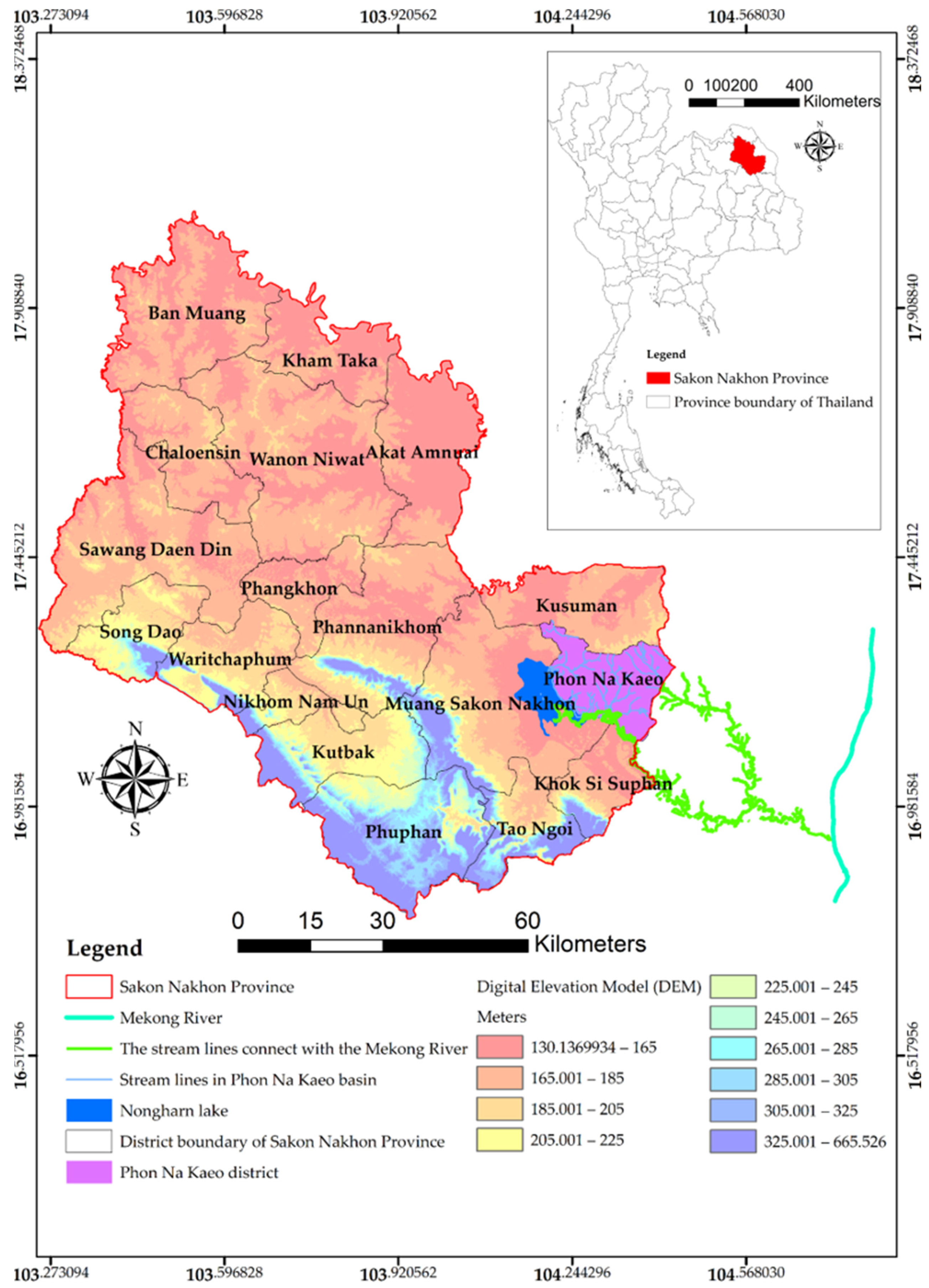
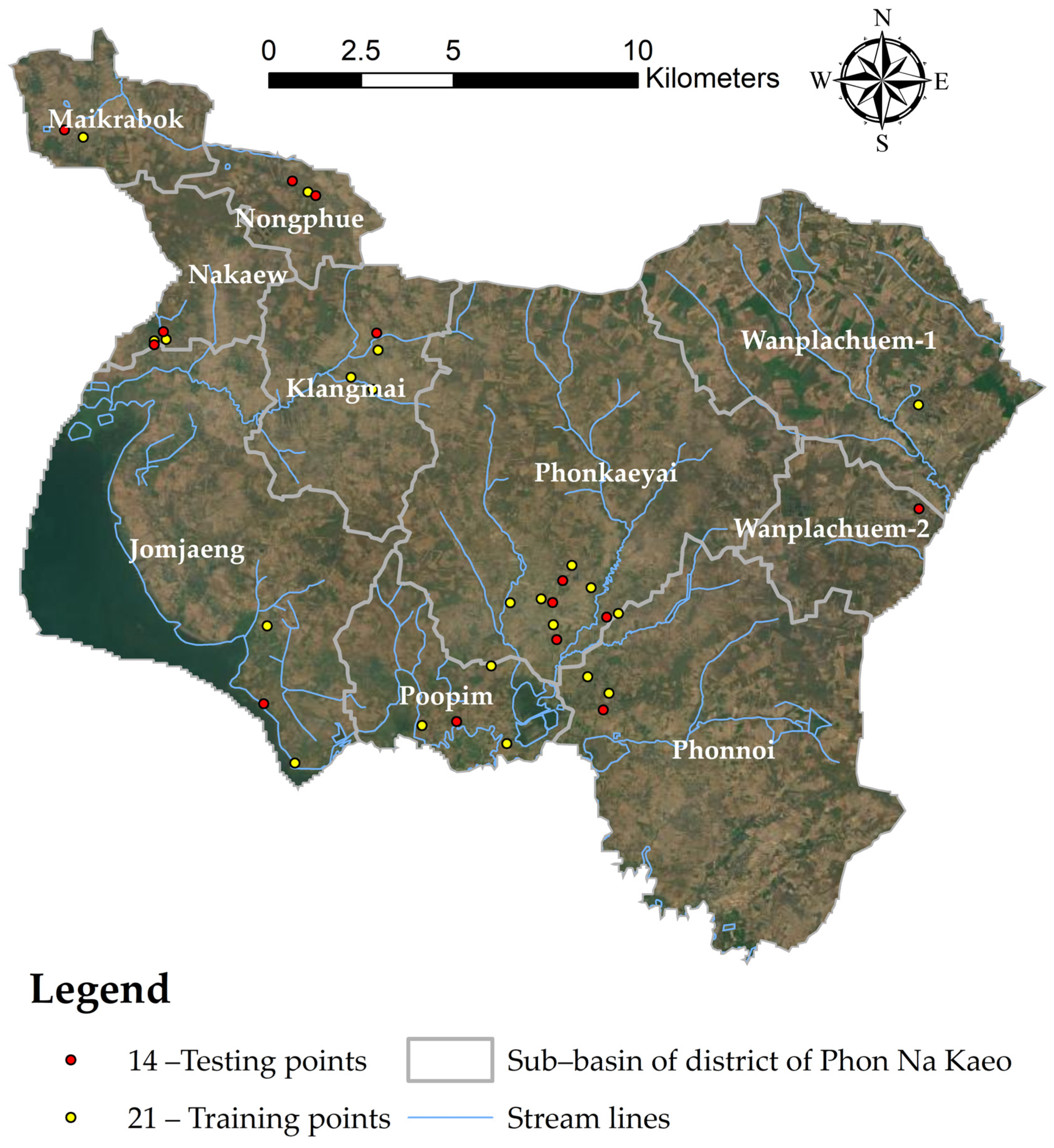
1.1. The Study Area
1.2. Datasets and Analyses
2. Materials and Methods
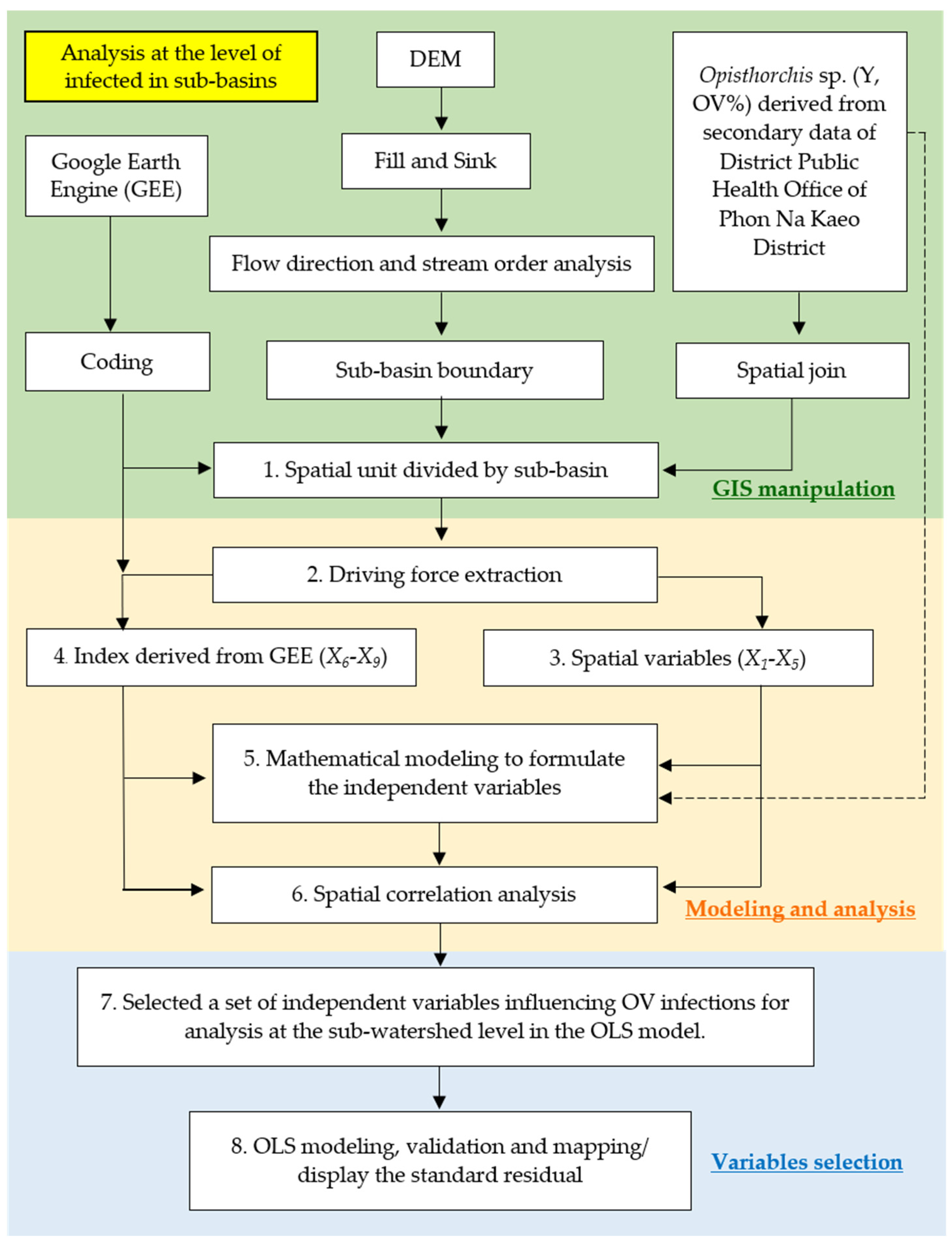
2.1. Ordinary Least Square (OLS) Approach for Spatial Modeling (Analysis at the Level of Infected in Sub-Basins)
- (1)
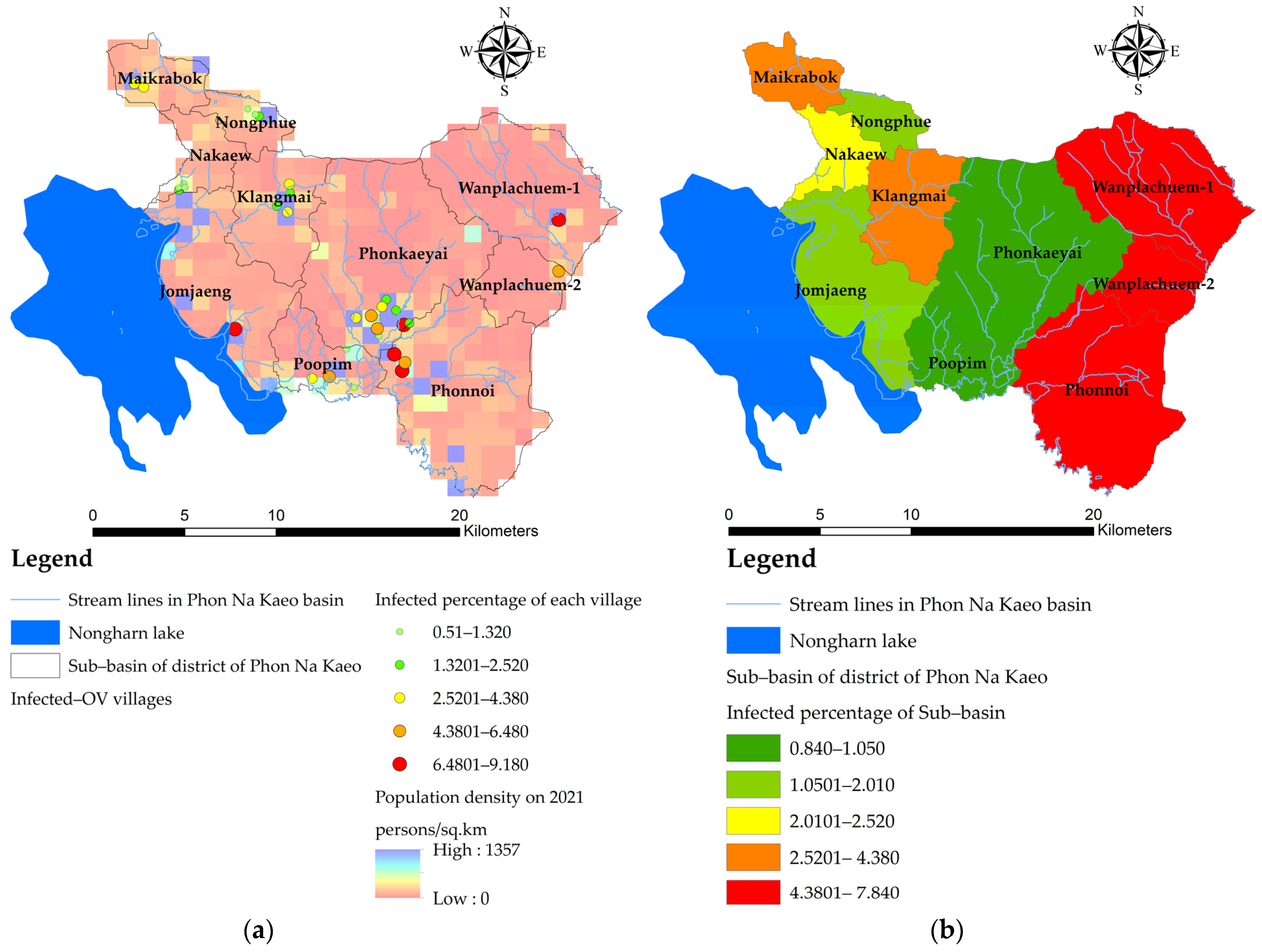
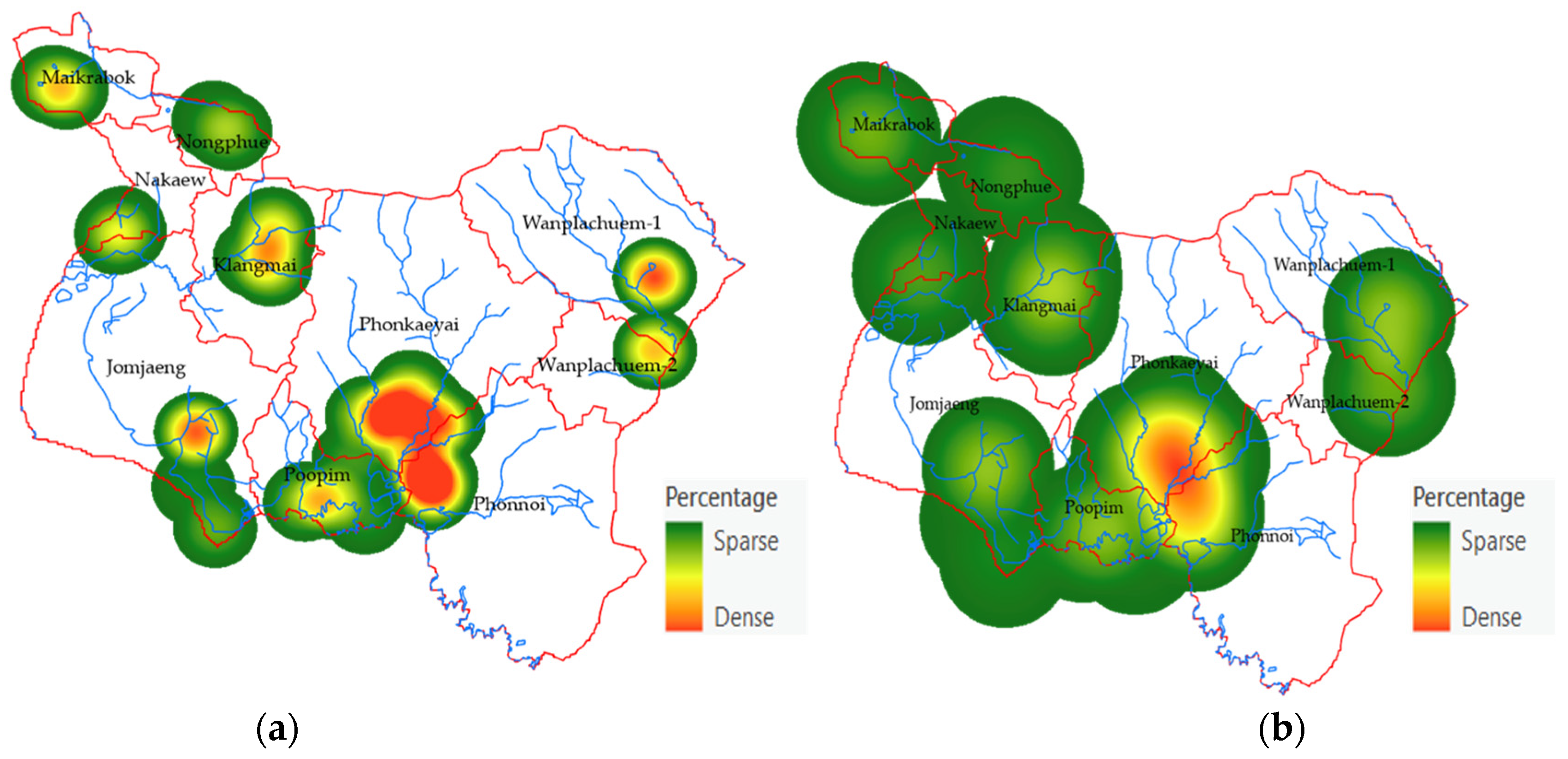
- The OLS model uses the principle of estimating the coefficients of the equation with the same squared method as the conventional linear model, but the creation of a variable dataset is a geostatistical statistic that can generate a dataset from a smaller sample but retain a Z value that is similar to the original Z value. The area that seems to be the ideal area for shellfish implantation is the buffer area away from the accumulated flow line of water [20]. The variable data are generated as points of location in the village where the OV data were surveyed. The dependent variable (Y,OV%) is the point data of the location that each village regularly used to find fish for the period 2019–2021, where fish samples were collected and tested for liver fluke infection. Points that represent the percentage of infected people are converted into raster data to reflect the continuous distribution of dependent variables and use the average of infected people to represent that sub-basin. The location data of infected villages are used to create density maps to ensure the continuity of infection. In this study, a heat map was created with a kernel density approach. The density is calculated using the kernel density method, the same algorithm used by the kernel density geoprocessing tool in ArcGIS pro.
- (2)
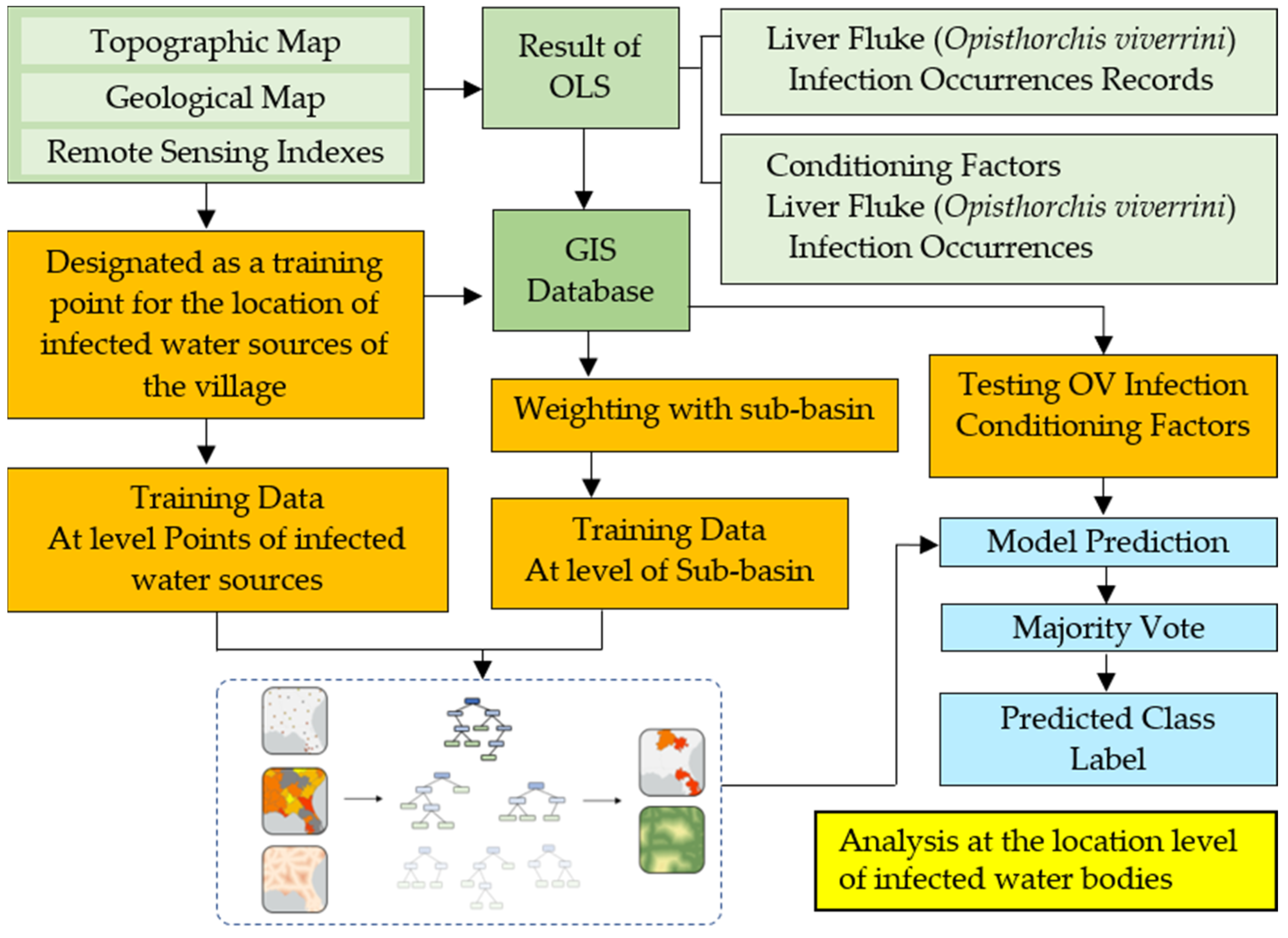
- When modeling the relationship between liver flukes, other types of parasites, and spatial factors, OLS uses a global model of spatial statistics, i.e., a model created specifically for each sub-basin, which allows for predicting liver flukes and other types of parasites and analyzing the relationships. The model serves to determine the coefficient of the relationship between the independent and dependent variables using the distance reciprocal weighting method, where OLS obtains a model to predict every unit area with a difference in coefficients [9,21,22]. OLS modeling must create a data layer based on this research, namely the percentage of liver fluke infection of the sub-basin region to be analyzed from 5 m DEM data, the import of independent variables, consisting of the index variables generated from the wavelength correlation of satellite images in mathematical functions, and other spatial factors, such as the distance from water bodies and roads; the detailed procedure is shown in Figure 4, and OLS is shown in Equation (1) [25].
- the interception point y (constant value);
- the regression coefficient or slope of the explanatory variable n at point i;
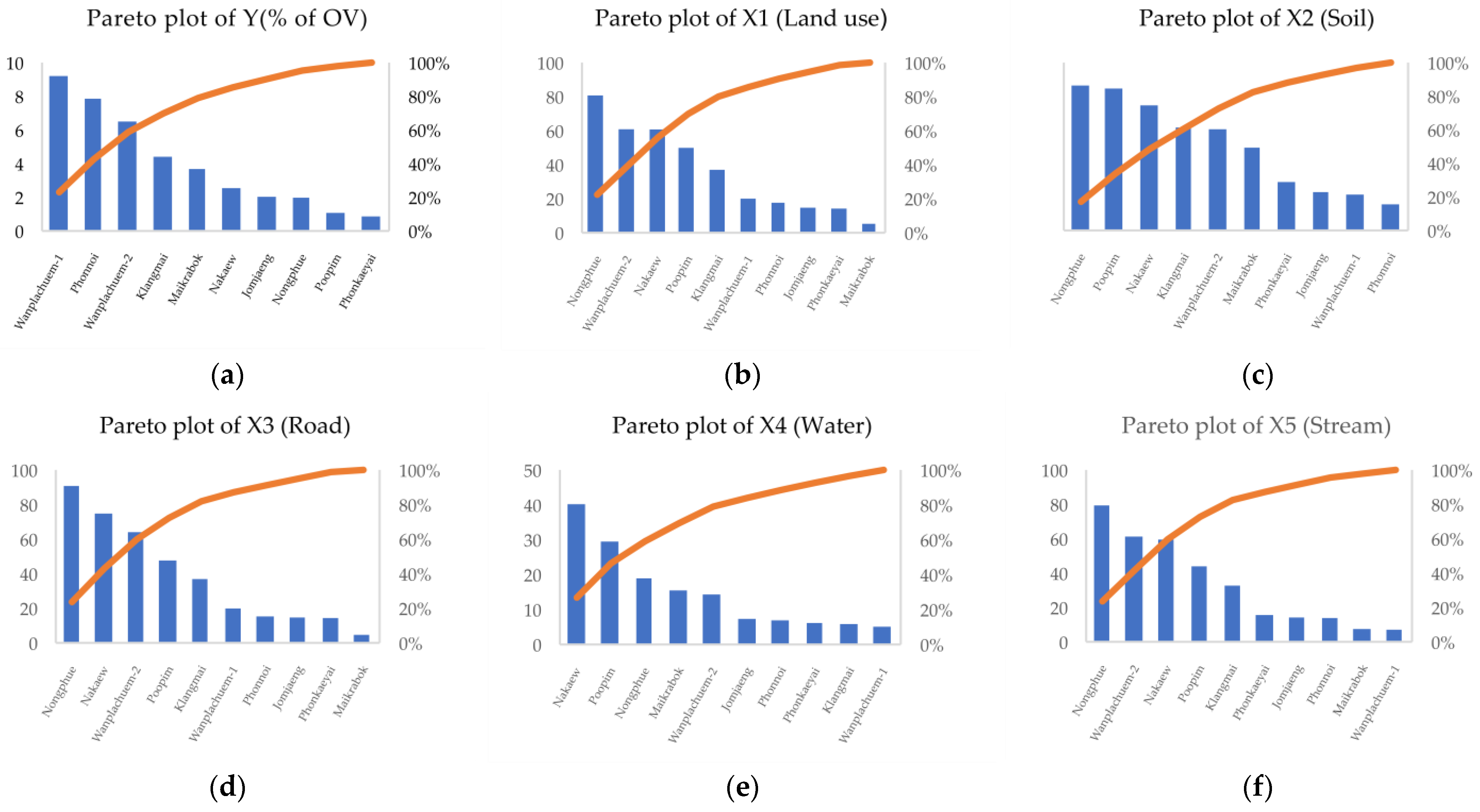
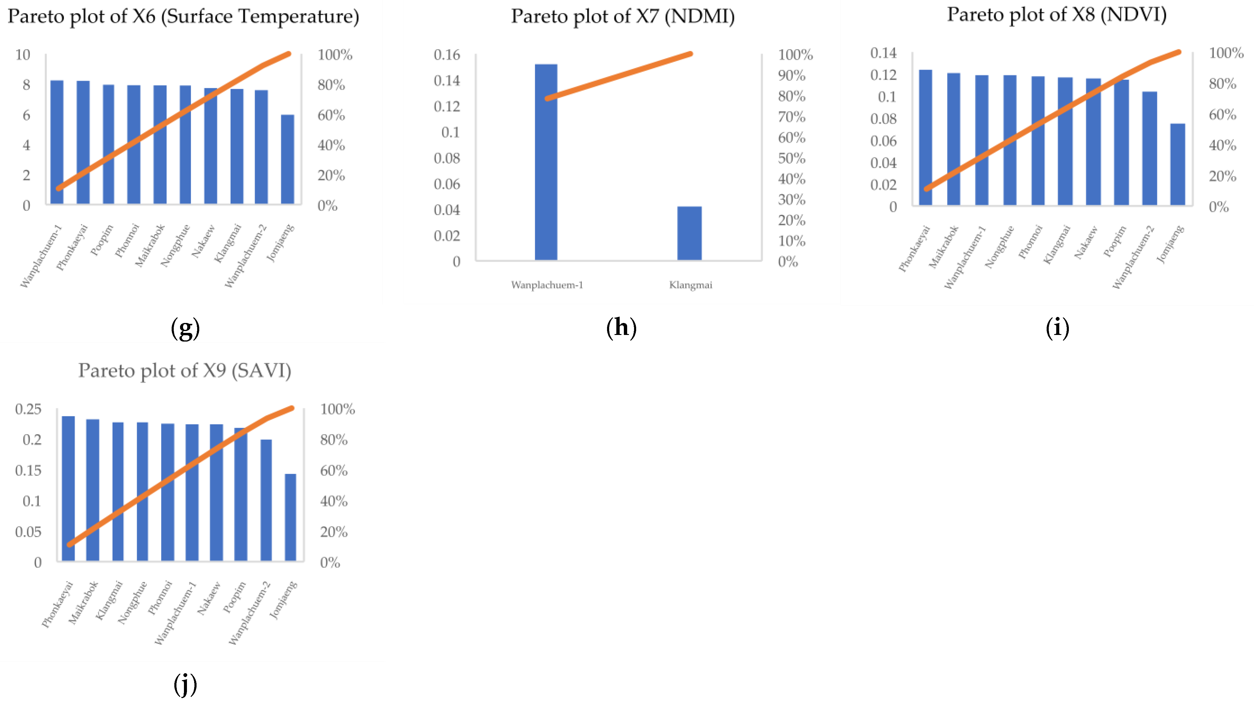
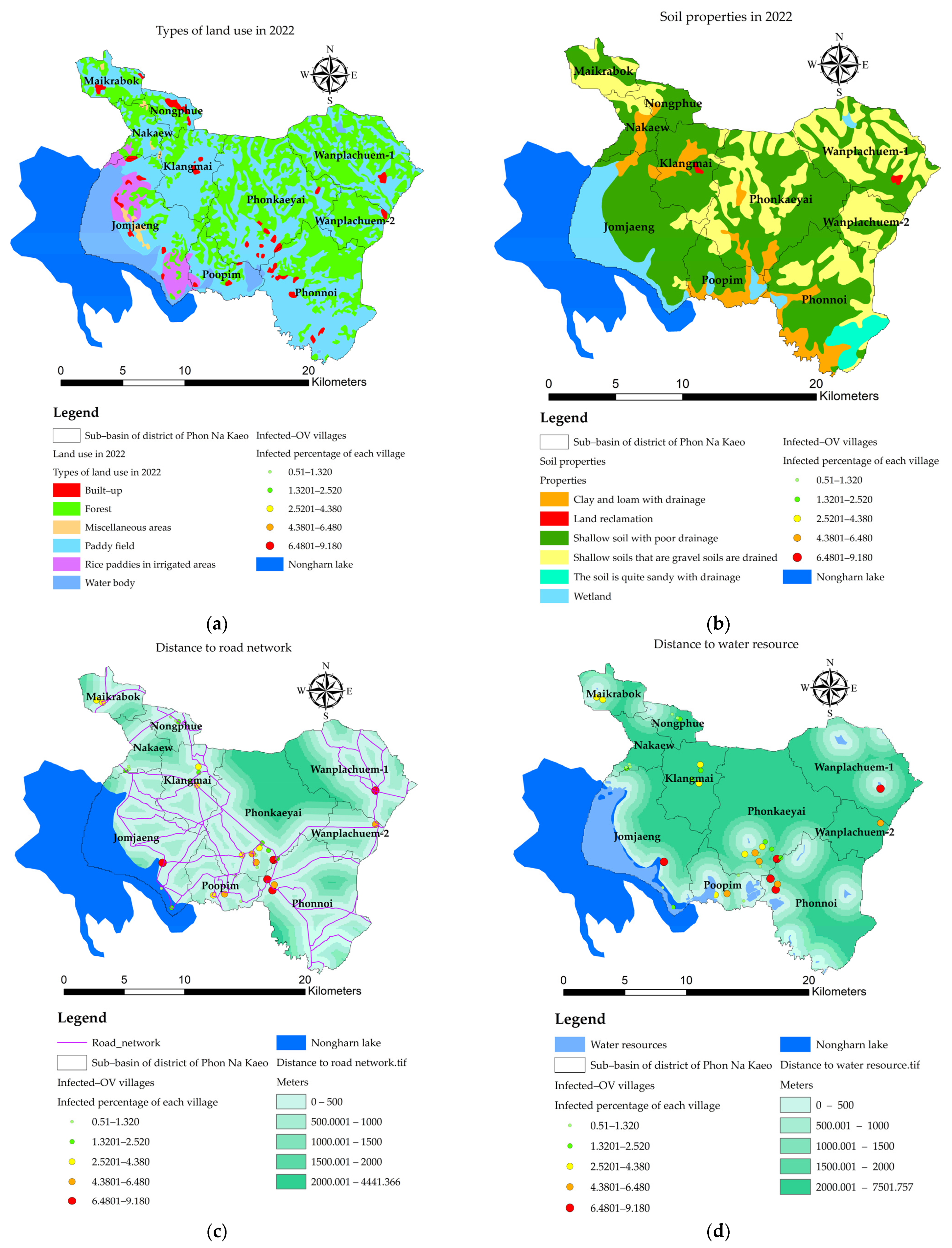
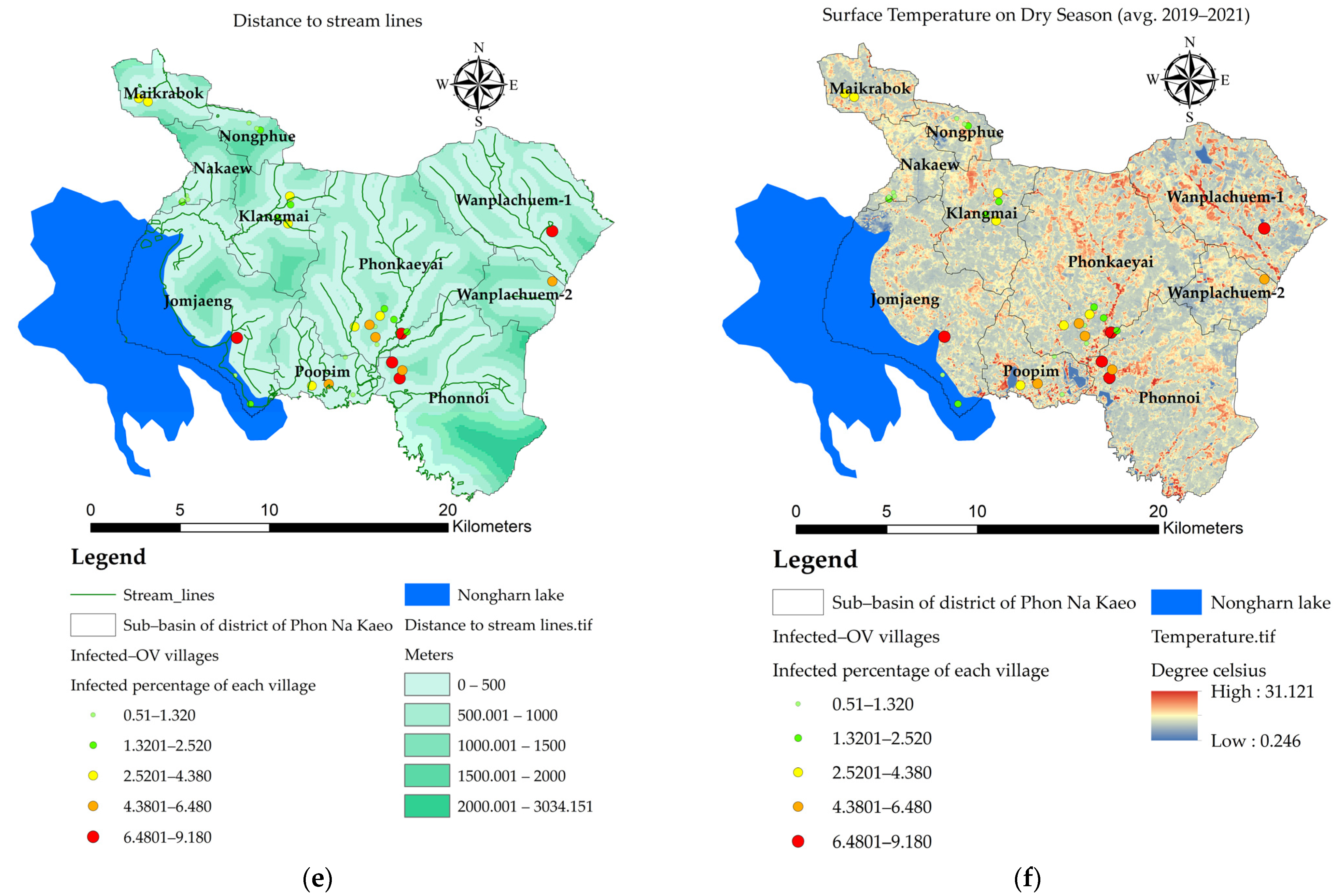
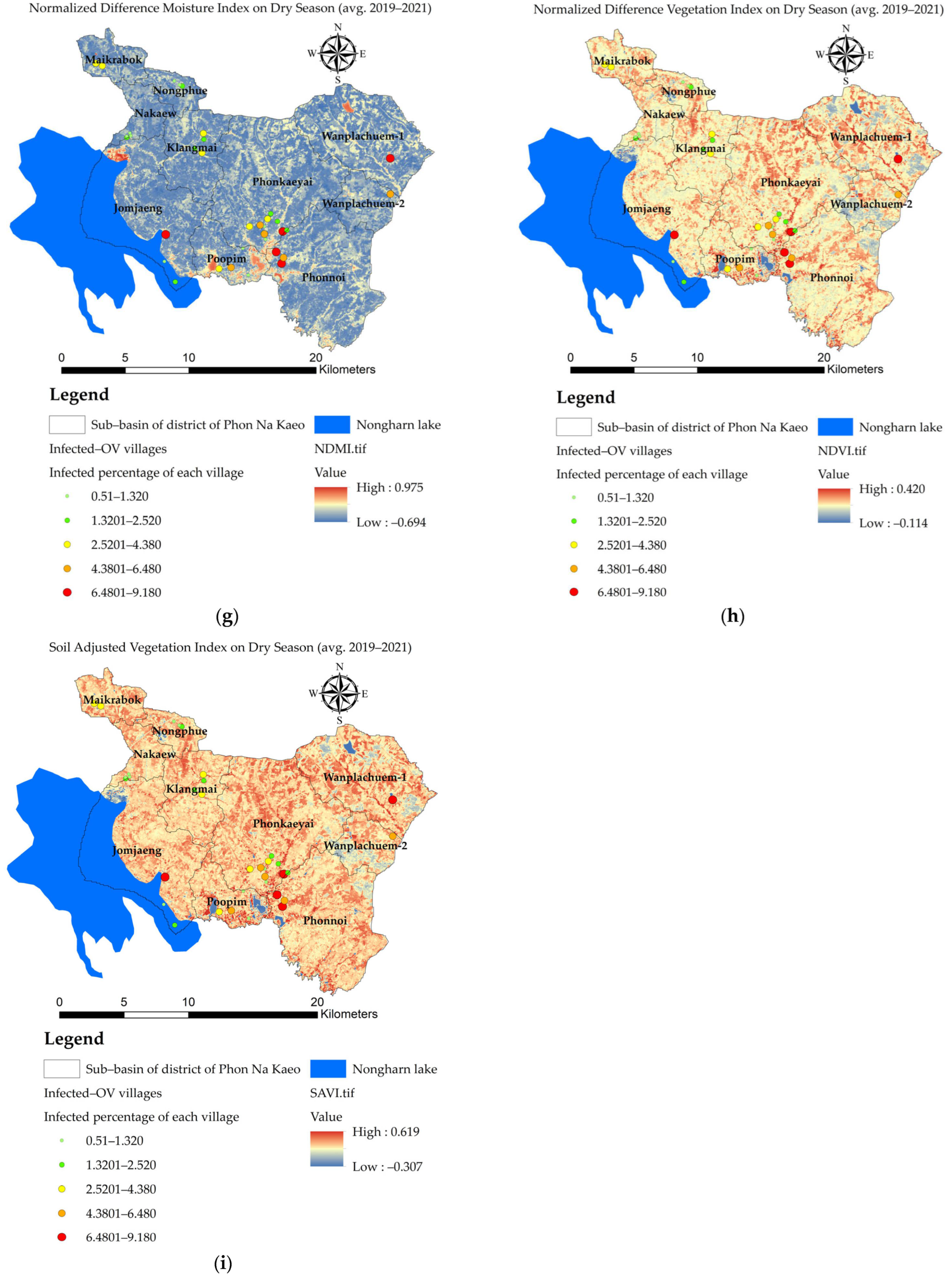
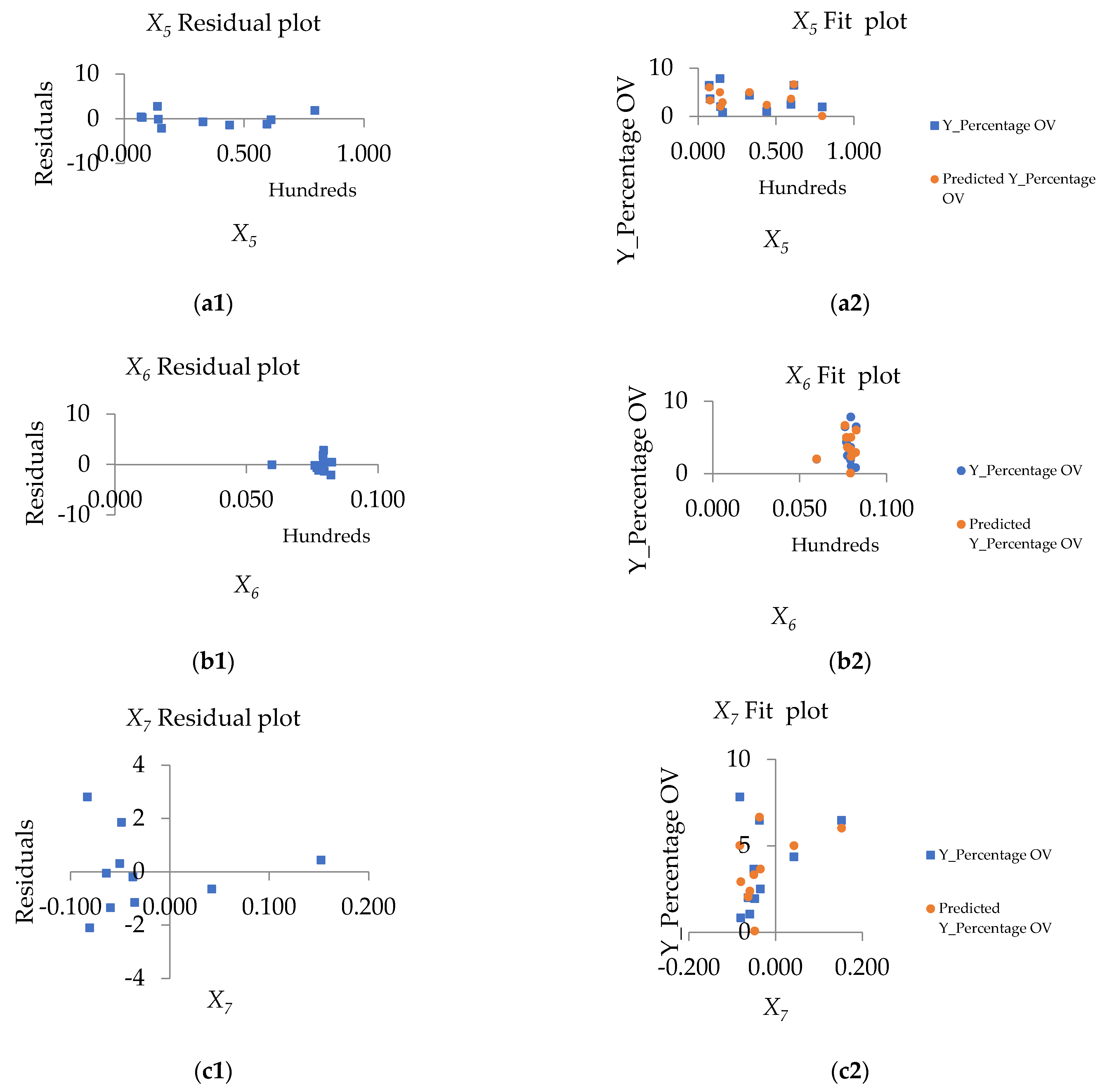
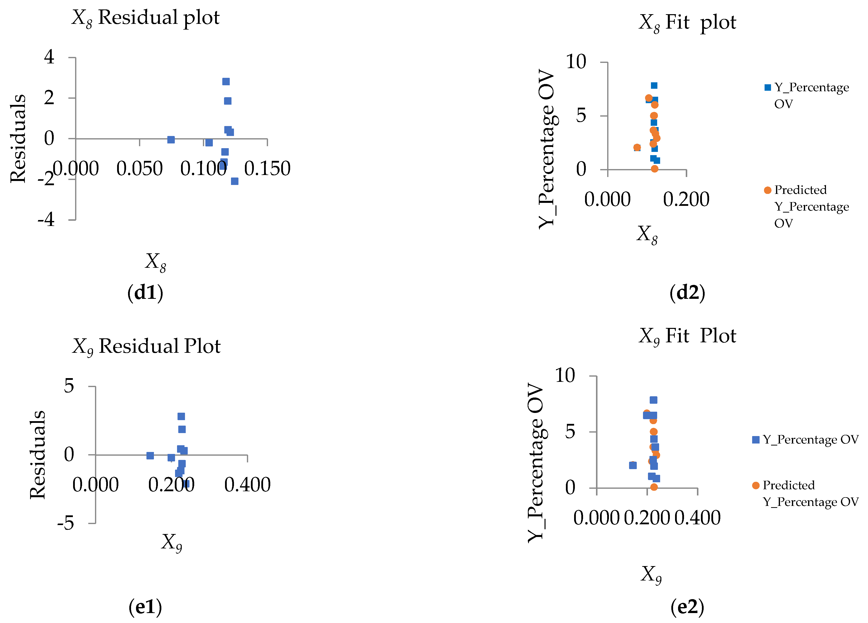
- the value of the variable n at point i. The X variable can be described as X1 (index of land-use types), X2 (index of soil drainage properties), X3 (distance index from the road network, X4 (distance index from surface water sources), X5 (distance index from the stream lines or flow accumulation lines), X6 (index of average surface temperature), X7 (average surface moisture index), X8 (average normalized difference vegetation index), and X9 (average soil-adjusted vegetation index);
- the error of the regression equation.
2.2. Independent Variable Modeling
2.3. Data Preparation for OLS and FCR Models
2.4. Forest-Based Classification and Regression (Analysis at the Location Level of Infected Water Bodies)
- Definition of the FCR for liver fluke (Opisthorchis viverrini) infection prediction
- Description of the pre-processing
- Dimension of the dataset
- Processor for feature selection
- Description of the different modeling tested and rationale behind the model construction
- Validation protocol to analyze FCR models’ performance
3. Results
3.1. Factor Selected for OLS with Liver Fluke Infection (Watershed Level)
3.2. Mapping the Spatial OV Infection (Y, Dependent Variable)
3.3. Mapping of the Independent Variables
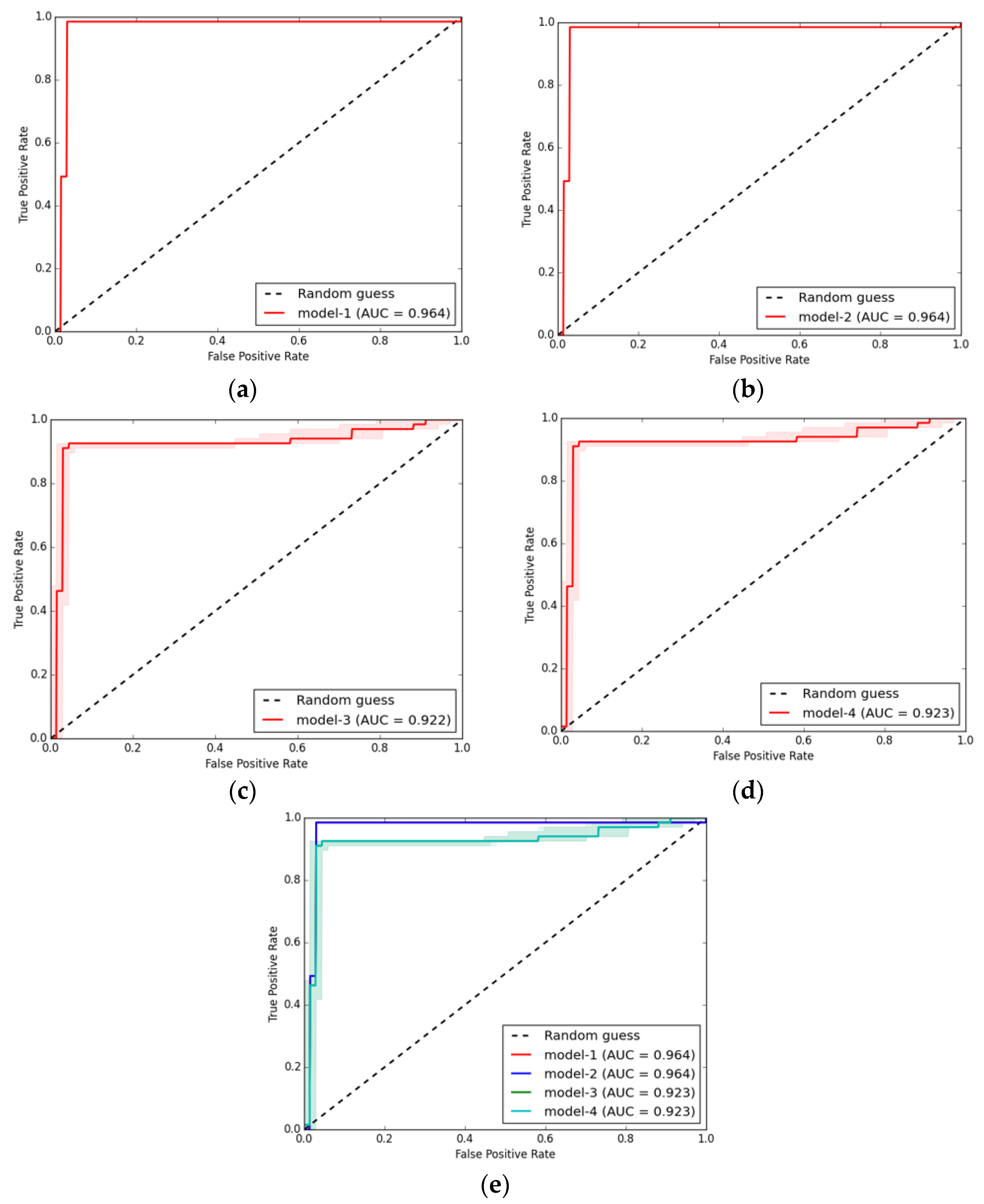
3.4. Spatial Prediction of OV-Infection Using Forest-Based Classification and Regression (FCR) (Location Level)
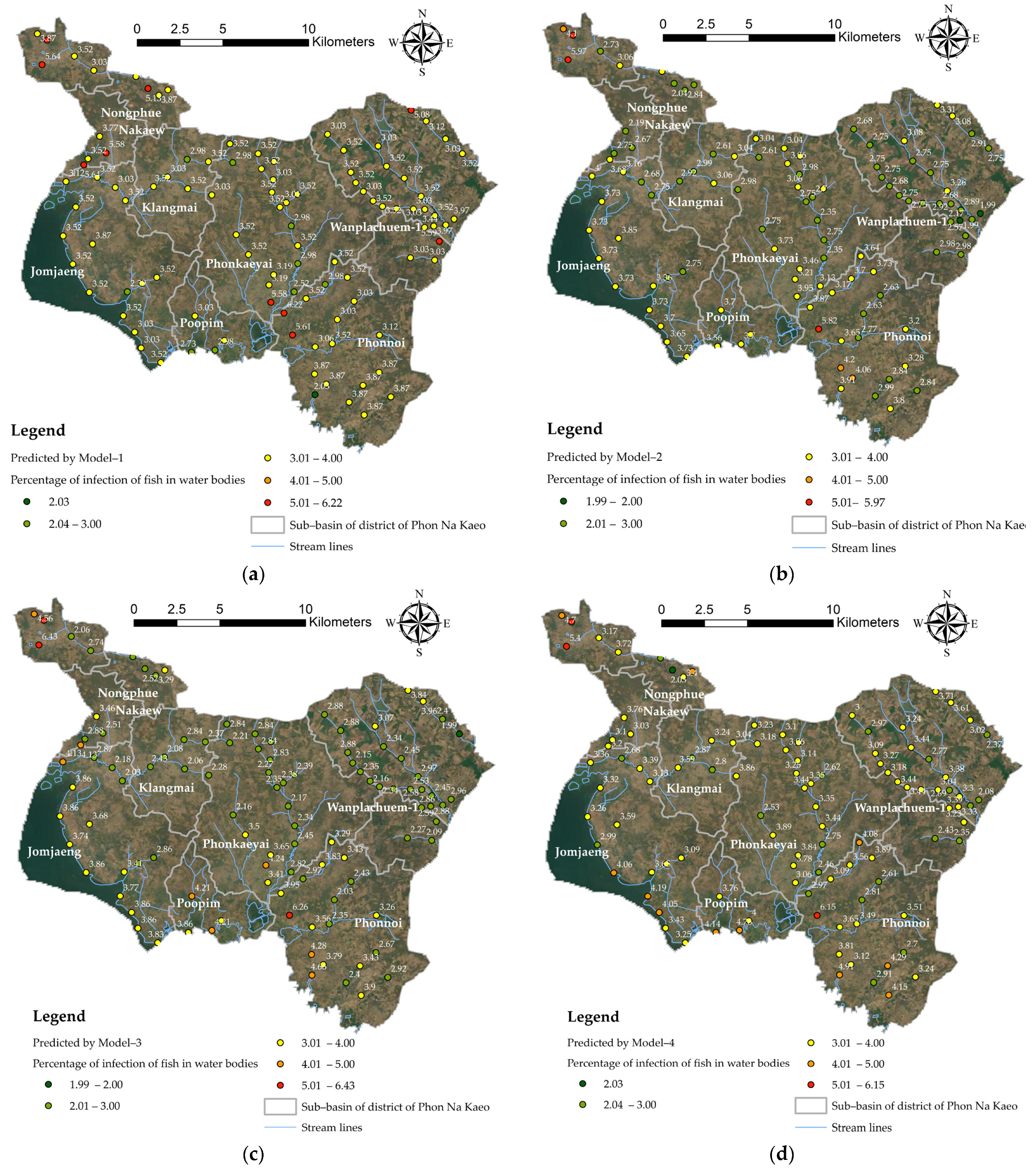
3.5. Spatial Prediction of OV-Infected
4. Discussion
4.1. Redundancy of Independent Variable Sets Associated with Spatial Liver Infection
4.2. Limitations of Spatial OLS Model
4.3. FCR Improvement Approach for Spatial Prediction
4.4. The Importance of the Single Variables to the Models
5. Conclusions
- An OLS model was developed in this study to track liver fluke infection. This spatial statistical model is suitable for analysis at the local process level, and the results were compared to confirm that Model 3 was more accurate and more appropriate than Model 1, Model 2, and Model 4. However, to make full use of the model, the spatial unit data layer should first be designed to separate the variables accordingly and independently [90,91,92]. Often, OLS models provide low coefficients of decision because sub-area unit assignments are not suitable. In this study, OLS could be used as a prototype for a method for analyzing spatial relationships with liver fluke infections by creating sub-basin units with continuous, adjacent boundaries. Local fluke case data should be continuously collected so that a curve can be created between the percentage of infected people and an independent set of variables. The factors used in this study are only prototypes of OLS model testing; in more advanced studies, spatial survey factors such as soil moisture in the field where mollusks are found should be used. Mathematical modeling is used to adjust database measures so that they can be measured together as an alternative approach to optimizing the prediction of the model [22]. Finally, the results of this study can guide the creation of spatial models at the scale of small watersheds to track spatial infections of liver flukes in other areas with similar watershed characteristics.
- Improving prediction at the position level by using machine learning and the FCR method: in order to improve performance when extracting values from explanatory training rasters and calculate the distances by using explanatory training distance features, consider training the model on 100% of the data without excluding data for testing, and choose to create output trained features [27,44]. Although the default number of trees parameter value is 100, this number is not data-driven. The number of trees needed increases with the complexity of the relationships between the explanatory variables, the size of the dataset, and the variable used to predict, in addition to variations in these variables. Increase the number of trees in the forest value and keep track of the out-of-bags (OOBs) or classification errors [93]. It is recommended to increase the number of trees by least three times up to at least 500 trees to best evaluate model performance. Tool execution time is highly sensitive to the number of variables used per tree. Using a small number of variables per tree decreases the chances of overfitting [27]; however, be sure to use many trees if the model is using a small number of variables per tree to improve model performance. In order to create a model that does not change in every run, a seed can be set in the random number generator environment setting. There will still be randomness in the model, but that randomness will be consistent between runs.
Supplementary Materials
Author Contributions
Funding
Institutional Review Board Statement
Informed Consent Statement
Data Availability Statement
Acknowledgments
Conflicts of Interest
References
- Geadkaew-Krenc, A.; Krenc, D.; Thanongsaksrikul, J.; Grams, R.; Phadungsil, W.; Glab-ampai, K.; Chantree, P.; Martviset, P. Production and Immunological Characterization of ScFv Specific to Epitope of Opisthorchis Viverrini Rhophilin-Associated Tail Protein 1-like (OvROPN1L). Trop. Med. Infect. Dis. 2023, 8, 160. [Google Scholar] [CrossRef] [PubMed]
- Perakanya, P.; Ungcharoen, R.; Worrabannakorn, S.; Ongarj, P.; Artchayasawat, A.; Boonmars, T.; Boueroy, P. Prevalence and Risk Factors of Opisthorchis Viverrini Infection in Sakon Nakhon Province, Thailand. Trop. Med. Infect. Dis. 2022, 7, 313. [Google Scholar] [CrossRef] [PubMed]
- Sadaow, L.; Rodpai, R.; Janwan, P.; Boonroumkaew, P.; Sanpool, O.; Thanchomnang, T.; Yamasaki, H.; Ittiprasert, W.; Mann, V.H.; Brindley, P.J.; et al. An Innovative Test for the Rapid Detection of Specific IgG Antibodies in Human Whole-Blood for the Diagnosis of Opisthorchis Viverrini Infection. Trop. Med. Infect. Dis. 2022, 7, 308. [Google Scholar] [CrossRef] [PubMed]
- Boonjaraspinyo, S.; Boonmars, T.; Ekobol, N.; Artchayasawat, A.; Sriraj, P.; Aukkanimart, R.; Pumhirunroj, B.; Sripan, P.; Songsri, J.; Juasook, A.; et al. Prevalence and Associated Risk Factors of Intestinal Parasitic Infections: A Population-Based Study in Phra Lap Sub-District, Mueang Khon Kaen District, Khon Kaen Province, Northeastern Thailand. Trop. Med. Infect. Dis. 2023, 8, 22. [Google Scholar] [CrossRef]
- Sripa, B.; Bethony, J.M.; Sithithaworn, P.; Kaewkes, S.; Mairiang, E.; Loukas, A.; Mulvenna, J.; Laha, T.; Hotez, P.J.; Brindley, P.J. Opisthorchiasis and Opisthorchis-Associated Cholangiocarcinoma in Thailand and Laos. Acta Trop. 2011, 120, S158–S168. [Google Scholar] [CrossRef]
- Prasongwatana, J.; Laummaunwai, P.; Boonmars, T.; Pinlaor, S. Viable Metacercariae of Opisthorchis viverrini in Northeastern Thai Cyprinid Fish Dishes—As Part of a Rational Program for Control of O. viverrini-Associated Cholangiocarcinoma. Parasitol. Res. 2013, 112, 1323–1327. [Google Scholar] [CrossRef]
- Sripa, B.; Kaewkes, S.; Sithithaworn, P.; Mairiang, E.; Laha, T.; Smout, M.; Pairojkul, C.; Bhudhisawasdi, V.; Tesana, S.; Thinkamrop, B.; et al. Liver Fluke Induces Cholangiocarcinoma. PLoS Med. 2007, 4, e201. [Google Scholar] [CrossRef]
- Sripa, B.; Brindley, P.J.; Mulvenna, J.; Laha, T.; Smout, M.J.; Mairiang, E.; Bethony, J.M.; Loukas, A. The Tumorigenic Liver Fluke Opisthorchis Viverrini–Multiple Pathways to Cancer. Trends Parasitol. 2012, 28, 395–407. [Google Scholar] [CrossRef]
- Sripa, B.; Tangkawattana, S.; Laha, T.; Kaewkes, S.; Mallory, F.F.; Smith, J.F.; Wilcox, B.A. Toward Integrated Opisthorchiasis Control in Northeast Thailand: The Lawa Project. Acta Trop. 2015, 141, 361–367. [Google Scholar] [CrossRef]
- Haswell-Elkins, M.R.; Satarug, S.; Elkins, D.B. Opisthorchis Viverrini Infection in Northeast Thailand and Its Relationship to Cholangiocarcinoma. J. Gastroenterol. Hepatol. 1992, 7, 538–548. [Google Scholar] [CrossRef]
- Mairiang, E.; Elkins, D.B.; Mairiang, P.; Chaiyakum, J.; Chamadol, N.; Loapaiboon, V.; Posri, S.; Sithithaworn, P.; Haswell-Elkins, M. Relationship between Intensity of Opisthorchis Viverrini Infection and Hepatobiliary Disease Detected by Ultrasonography. J. Gastroenterol. Hepatol. 1992, 7, 17–21. [Google Scholar] [CrossRef] [PubMed]
- Pumhirunroj, B.; Aukkanimart, R. Liver Fluke-Infected Cyprinoid Fish in Northeastern Thailand (2016–2017). Southeast Asian J. Trop. Med. Public Health 2017, 51, 1–7. [Google Scholar]
- Pinlaor, S.; Onsurathum, S.; Boonmars, T.; Pinlaor, P.; Hongsrichan, N.; Chaidee, A.; Haonon, O.; Limviroj, W.; Tesana, S.; Kaewkes, S.; et al. Distribution and Abundance of Opisthorchis Viverrini Metacercariae in Cyprinid Fish in Northeastern Thailand. Korean J. Parasitol. 2013, 51, 703–710. [Google Scholar] [CrossRef] [PubMed]
- Suwannatrai, A.T.; Thinkhamrop, K.; Clements, A.C.A.; Kelly, M.; Suwannatrai, K.; Thinkhamrop, B.; Khuntikeo, N.; Gray, D.J.; Wangdi, K. Bayesian Spatial Analysis of Cholangiocarcinoma in Northeast Thailand. Sci. Rep. 2019, 9, 14263. [Google Scholar] [CrossRef] [PubMed]
- Hasegawa, S.; Ikai, I.; Fujii, H.; Hatano, E.; Shimahara, Y. Surgical Resection of Hilar Cholangiocarcinoma: Analysis of Survival and Postoperative Complications. World J. Surg. 2007, 31, 1258–1265. [Google Scholar] [CrossRef] [PubMed]
- Thinkhamrop, K.; Suwannatrai, A.T.; Chamadol, N.; Khuntikeo, N.; Thinkhamrop, B.; Sarakarn, P.; Gray, D.J.; Wangdi, K.; Clements, A.C.A.; Kelly, M. Spatial Analysis of Hepatobiliary Abnormalities in a Population at High-Risk of Cholangiocarcinoma in Thailand. Sci. Rep. 2020, 10, 16855. [Google Scholar] [CrossRef]
- Pratumchart, K.; Suwannatrai, K.; Sereewong, C.; Thinkhamrop, K.; Chaiyos, J.; Boonmars, T.; Suwannatrai, A.T. Ecological Niche Model Based on Maximum Entropy for Mapping Distribution of Bithynia Siamensis Goniomphalos, First Intermediate Host Snail of Opisthorchis Viverrini in Thailand. Acta Trop. 2019, 193, 183–191. [Google Scholar] [CrossRef]
- Sriamporn, S.; Pisani, P.; Pipitgool, V.; Suwanrungruang, K.; Kamsa-ard, S.; Parkin, D.M. Prevalence of Opisthorchis viverrini infection and incidence of cholangiocarcinoma in Khon Kaen, Northeast Thailand. Trop. Med. Int. Health 2004, 9, 588–594. [Google Scholar] [CrossRef]
- Martviset, P.; Phadungsil, W.; Na-Bangchang, K.; Sungkhabut, W.; Panupornpong, T.; Prathaphan, P.; Torungkitmangmi, N.; Chaimon, S.; Wangboon, C.; Jamklang, M.; et al. Current Prevalence and Geographic Distribution of Helminth Infections in the Parasitic Endemic Areas of Rural Northeastern Thailand. BMC Public Health 2023, 23, 448. [Google Scholar] [CrossRef]
- Littidej, P.; Buasri, N. Built-up Growth Impacts on Digital Elevation Model and Flood Risk Susceptibility Prediction in Muaeng District, Nakhon Ratchasima (Thailand). Water 2019, 11, 1496. [Google Scholar] [CrossRef]
- Littidej, P.; Uttha, T.; Pumhirunroj, B. Spatial Predictive Modeling of the Burning of Sugarcane Plots in Northeast Thailand with Selection of Factor Sets Using a GWR Model and Machine Learning Based on an ANN-CA. Symmetry 2022, 14, 1989. [Google Scholar] [CrossRef]
- Prasertsri, N.; Littidej, P. Spatial Environmental Modeling for Wildfire Progression Accelerating Extent Analysis Using Geo-Informatics. Pol. J. Environ. Stud. 2020, 29, 3249–3261. [Google Scholar] [CrossRef]
- Lu, B.; Charlton, M.; Fotheringham, A.S. Geographically Weighted Regression Using a Non-Euclidean Distance Metric with a Study on London House Price Data. Procedia Environ. Sci. 2011, 7, 92–97. [Google Scholar] [CrossRef]
- Lu, B.; Charlton, M.; Harris, P.; Fotheringham, A.S. Geographically Weighted Regression with a Non-Euclidean Distance Metric: A Case Study Using Hedonic House Price Data. Int. J. Geogr. Inf. Sci. 2014, 28, 660–681. [Google Scholar] [CrossRef]
- Fotheringham, A.; Charlton, M. Geographically Geographically Weighted Weighted Regression Regression A Stewart Fotheringham. Geogr. Anal. 2014, 28, 281–298. [Google Scholar]
- Hussain, M.A.; Chen, Z.; Zheng, Y.; Shoaib, M.; Shah, S.U.; Ali, N.; Afzal, Z. Landslide Susceptibility Mapping Using Machine Learning Algorithm Validated by Persistent Scatterer In-SAR Technique. Sensors 2022, 22, 3119. [Google Scholar] [CrossRef] [PubMed]
- Achour, Y.; Pourghasemi, H.R. How Do Machine Learning Techniques Help in Increasing Accuracy of Landslide Susceptibility Maps? Geosci. Front. 2020, 11, 871–883. [Google Scholar] [CrossRef]
- Kumar, R.; Anbalagan, R. Landslide Susceptibility Mapping Using Analytical Hierarchy Process (AHP) in Tehri Reservoir Rim Region, Uttarakhand. J. Geol. Soc. India 2016, 87, 271–286. [Google Scholar] [CrossRef]
- Tengtrairat, N.; Woo, W.L.; Parathai, P.; Aryupong, C.; Jitsangiam, P.; Rinchumphu, D. Automated Landslide-Risk Prediction Using Web GIS and Machine Learning Models. Sensors 2021, 21, 4620. [Google Scholar] [CrossRef]
- Park, S.; Choi, C.; Kim, B.; Kim, J. Landslide Susceptibility Mapping Using Frequency Ratio, Analytic Hierarchy Process, Logistic Regression, and Artificial Neural Network Methods at the Inje Area, Korea. Environ. Earth Sci. 2013, 68, 1443–1464. [Google Scholar] [CrossRef]
- Tien Bui, D.; Pradhan, B.; Lofman, O.; Revhaug, I. Landslide Susceptibility Assessment in Vietnam Using Support Vector Machines, Decision Tree, and Naïve Bayes Models. Math. Probl. Eng. 2012, 2012, 974638. [Google Scholar] [CrossRef]
- Mandal, S.; Mandal, K. Modeling and Mapping Landslide Susceptibility Zones Using GIS Based Multivariate Binary Logistic Regression (LR) Model in the Rorachu River Basin of Eastern Sikkim Himalaya, India. Model. Earth Syst. Environ. 2018, 4, 69–88. [Google Scholar] [CrossRef]
- Pourghasemi, H.R.; Rahmati, O. Prediction of the Landslide Susceptibility: Which Algorithm, Which Precision? Catena 2018, 162, 177–192. [Google Scholar] [CrossRef]
- Youssef, A.M.; Pourghasemi, H.R.; Pourtaghi, Z.S.; Al-Katheeri, M.M. Landslide Susceptibility Mapping Using Random Forest, Boosted Regression Tree, Classification and Regression Tree, and General Linear Models and Comparison of Their Performance at Wadi Tayyah Basin, Asir Region, Saudi Arabia. Landslides 2016, 13, 839–856. [Google Scholar] [CrossRef]
- Rossi, M.; Guzzetti, F.; Reichenbach, P.; Mondini, A.C.; Peruccacci, S. Optimal Landslide Susceptibility Zonation Based on Multiple Forecasts. Geomorphology 2010, 114, 129–142. [Google Scholar] [CrossRef]
- Park, S.; Kim, J. Landslide Susceptibility Mapping Based on Random Forest and Boosted Regression Tree Models, and a Comparison of Their Performance. Appl. Sci. 2019, 9, 942. [Google Scholar] [CrossRef]
- Sevgen, E.; Kocaman, S.; Nefeslioglu, H.A.; Gokceoglu, C. Photogrammetric Techniques for Landslide Susceptibility Mapping with Logistic Regression. Sensors 2019, 19, 3940. [Google Scholar] [CrossRef]
- Pérez-Díaz, P.; Martín-Dorta, N.; Gutiérrez-García, F.J. Construction Labour Measurement in Reinforced Concrete Floating Caissons in Maritime Ports. Civ. Eng. J. 2022, 8, 195–208. [Google Scholar] [CrossRef]
- Hussain, M.A.; Chen, Z.; Wang, R.; Shoaib, M. Ps-Insar-Based Validated Landslide Susceptibility Mapping along Karakorum Highway, Pakistan. Remote Sens. 2021, 13, 4129. [Google Scholar] [CrossRef]
- Taalab, K.; Cheng, T.; Zhang, Y. Mapping Landslide Susceptibility and Types Using Random Forest. Big Earth Data 2018, 2, 159–178. [Google Scholar] [CrossRef]
- Conoscenti, C.; Ciaccio, M.; Caraballo-Arias, N.A.; Gómez-Gutiérrez, Á.; Rotigliano, E.; Agnesi, V. Assessment of Susceptibility to Earth-Flow Landslide Using Logistic Regression and Multivariate Adaptive Regression Splines: A Case of the Belice River Basin (Western Sicily, Italy). Geomorphology 2015, 242, 49–64. [Google Scholar] [CrossRef]
- Felicísimo, Á.M.; Cuartero, A.; Remondo, J.; Quirós, E. Mapping Landslide Susceptibility with Logistic Regression, Multiple Adaptive Regression Splines, Classification and Regression Trees, and Maximum Entropy Methods: A Comparative Study. Landslides 2013, 10, 175–189. [Google Scholar] [CrossRef]
- Vorpahl, P.; Elsenbeer, H.; Märker, M.; Schröder, B. How Can Statistical Models Help to Determine Driving Factors of Landslides? Ecol. Model. 2012, 239, 27–39. [Google Scholar] [CrossRef]
- Ghasemian, B.; Shahabi, H.; Shirzadi, A.; Al-Ansari, N.; Jaafari, A.; Kress, V.; Renoud, S.; Ramadhan, A.; Geertsema, M. A Robust Deep-Learning Model for Landslide Susceptibility Mapping. Sensors 2022, 22, 1573. [Google Scholar] [CrossRef] [PubMed]
- Ma, J.; Wang, Y.; Niu, X.; Jiang, S.; Liu, Z. A Comparative Study of Mutual Information-Based Input Variable Selection Strategies for the Displacement Prediction of Seepage-Driven Landslides Using Optimized Support Vector Regression. Stoch. Environ. Res. Risk Assess. 2022, 36, 3109–3129. [Google Scholar] [CrossRef]
- Kalantar, B.; Pradhan, B.; Naghibi, S.A.; Motevalli, A.; Mansor, S. Assessment of the Effects of Training Data Selection on the Landslide Susceptibility Mapping: A Comparison between Support Vector Machine (SVM), Logistic Regression (LR) and Artificial Neural Networks (ANN). Geomat. Nat. Hazards Risk 2018, 9, 49–69. [Google Scholar] [CrossRef]
- Pham, B.T.; Tien Bui, D.; Pourghasemi, H.R.; Indra, P.; Dholakia, M.B. Landslide Susceptibility Assesssment in the Uttarakhand Area (India) Using GIS: A Comparison Study of Prediction Capability of Naïve Bayes, Multilayer Perceptron Neural Networks, and Functional Trees Methods. Theor. Appl. Climatol. 2017, 128, 255–273. [Google Scholar] [CrossRef]
- Pham, B.T.; Pradhan, B.; Tien Bui, D.; Prakash, I.; Dholakia, M.B. A Comparative Study of Different Machine Learning Methods for Landslide Susceptibility Assessment: A Case Study of Uttarakhand Area (India). Environ. Model. Softw. 2016, 84, 240–250. [Google Scholar] [CrossRef]
- Mehrabi, M.; Pradhan, B.; Moayedi, H. Optimizing an Adaptive Neuro-Fuzzy Inference System for Spatial Prediction of Landslide Susceptibility Using Four State-of-the-Art Metaheuristic Techniques. Sensors 2020, 20, 1723. [Google Scholar] [CrossRef]
- Dehnavi, A.; Aghdam, I.N.; Pradhan, B.; Morshed Varzandeh, M.H. A New Hybrid Model Using Step-Wise Weight Assessment Ratio Analysis (SWARA) Technique and Adaptive Neuro-Fuzzy Inference System (ANFIS) for Regional Landslide Hazard Assessment in Iran. Catena 2015, 135, 122–148. [Google Scholar] [CrossRef]
- Aghdam, I.N.; Varzandeh, M.H.M.; Pradhan, B. Landslide Susceptibility Mapping Using an Ensemble Statistical Index (Wi) and Adaptive Neuro-Fuzzy Inference System (ANFIS) Model at Alborz Mountains (Iran). Environ. Earth Sci. 2016, 75, 553. [Google Scholar] [CrossRef]
- Kumar, R.; Anbalagan, R. Landslide Susceptibility Zonation in Part of Tehri Reservoir Region Using Frequency Ratio, Fuzzy Logic and GIS. J. Earth Syst. Sci. 2015, 124, 431–448. [Google Scholar] [CrossRef]
- Charandabi, S.E.; Kamyar, K. Prediction of Cryptocurrency Price Index Using Artificial Neural Networks: A Survey of the Literature. Eur. J. Bus. Manag. Res. 2021, 6, 17–20. [Google Scholar] [CrossRef]
- Roshani, M.; Sattari, M.A.; Muhammad Ali, P.J.; Roshani, G.H.; Nazemi, B.; Corniani, E.; Nazemi, E. Application of GMDH Neural Network Technique to Improve Measuring Precision of a Simplified Photon Attenuation Based Two-Phase Flowmeter. Flow Meas. Instrum. 2020, 75, 101804. [Google Scholar] [CrossRef]
- Moayedi, H.; Abdolreza, O.; Bui, D.T.; Foong, L.K. Spatial Landslide Susceptibility Assessment Based on Novel Neural-Metaheuristic Geographic Information System Based Ensembles. Sensors 2019, 19, 4698. [Google Scholar] [CrossRef] [PubMed]
- Bui, D.T.; Moayedi, H.; Kalantar, B.; Osouli, A.; Pradhan, B.; Nguyen, H.; Rashid, A.S.A. A Novel Swarm Intelligence—Harris Hawks Optimization for Spatial Assessment of Landslide Susceptibility. Sensors 2019, 19, 3590. [Google Scholar] [CrossRef] [PubMed]
- Arnone, E.; Francipane, A.; Scarbaci, A.; Puglisi, C.; Noto, L.V. Effect of Raster Resolution and Polygon-Conversion Algorithm on Landslide Susceptibility Mapping. Environ. Model. Softw. 2016, 84, 467–481. [Google Scholar] [CrossRef]
- Aditian, A.; Kubota, T.; Shinohara, Y. Comparison of GIS-Based Landslide Susceptibility Models Using Frequency Ratio, Logistic Regression, and Artificial Neural Network in a Tertiary Region of Ambon, Indonesia. Geomorphology 2018, 318, 101–111. [Google Scholar] [CrossRef]
- Kornejady, A.; Ownegh, M.; Bahremand, A. Landslide Susceptibility Assessment Using Maximum Entropy Model with Two Different Data Sampling Methods. Catena 2017, 152, 144–162. [Google Scholar] [CrossRef]
- Park, N.-W. Using Maximum Entropy Modeling for Landslide Susceptibility Mapping with Multiple Geoenvironmental Data Sets. Environ. Earth Sci. 2015, 73, 937–949. [Google Scholar] [CrossRef]
- Dang, V.H.; Hoang, N.D.; Nguyen, L.M.D.; Bui, D.T.; Samui, P. A Novel GIS-Based Random Forest Machine Algorithm for the Spatial Prediction of Shallow Landslide Susceptibility. Forests 2020, 11, 118. [Google Scholar] [CrossRef]
- Wu, X.; Ren, F.; Niu, R. Landslide Susceptibility Assessment Using Object Mapping Units, Decision Tree, and Support Vector Machine Models in the Three Gorges of China. Environ. Earth Sci. 2014, 71, 4725–4738. [Google Scholar] [CrossRef]
- Merghadi, A.; Yunus, A.P.; Dou, J.; Whiteley, J.; ThaiPham, B.; Bui, D.T.; Avtar, R.; Abderrahmane, B. Machine Learning Methods for Landslide Susceptibility Studies: A Comparative Overview of Algorithm Performance. Earth Sci. Rev. 2020, 207, 103225. [Google Scholar] [CrossRef]
- Sahin, E.K. Comparative Analysis of Gradient Boosting Algorithms for Landslide Susceptibility Mapping. Geocarto Int. 2022, 37, 2441–2465. [Google Scholar] [CrossRef]
- Nohani, E.; Moharrami, M.; Sharafi, S.; Khosravi, K.; Pradhan, B.; Pham, B.T.; Lee, S.; Melesse, A.M. Landslide Susceptibility Mapping Using Different GIS-Based Bivariate Models. Water 2019, 11, 1402. [Google Scholar] [CrossRef]
- Pourghasemi, H.R.; Gayen, A.; Panahi, M.; Rezaie, F.; Blaschke, T. Multi-Hazard Probability Assessment and Mapping in Iran. Sci. Total Environ. 2019, 692, 556–571. [Google Scholar] [CrossRef]
- Yan, F.; Zhang, Q.; Ye, S.; Ren, B. A Novel Hybrid Approach for Landslide Susceptibility Mapping Integrating Analytical Hierarchy Process and Normalized Frequency Ratio Methods with the Cloud Model. Geomorphology 2019, 327, 170–187. [Google Scholar] [CrossRef]
- Suwannahitatorn, P.; Webster, J.; Riley, S.; Mungthin, M.; Donnelly, C.A. Uncooked Fish Consumption among Those at Risk of Opisthorchis Viverrini Infection in Central Thailand. PLoS ONE 2019, 14, e0211540. [Google Scholar] [CrossRef]
- Sripa, B.; Kaewkes, S.; Intapan, P.M.; Maleewong, W.; Brindley, P.J. Chapter 11—Food-Borne Trematodiases in Southeast Asia: Epidemiology, Pathology, Clinical Manifestation and Control. In Important Helminth Infections in Southeast Asia: Diversity and Potential for Control and Elimination, Part A; Zhou, X.-N., Bergquist, R., Olveda, R., Utzinger, J.B.T.-A., Eds.; Academic Press: Cambridge, MA, USA, 2010; Volume 72, pp. 305–350. ISBN 0065-308X. [Google Scholar]
- Qian, M.-B.; Utzinger, J.; Keiser, J.; Zhou, X.-N. Clonorchiasis. Lancet 2016, 387, 800–810. [Google Scholar] [CrossRef]
- Brindley, P.J.; Bachini, M.; Ilyas, S.I.; Khan, S.A.; Loukas, A.; Sirica, A.E.; Teh, B.T.; Wongkham, S.; Gores, G.J. Cholangiocarcinoma. Nat. Rev. Dis. Prim. 2021, 7, 65. [Google Scholar] [CrossRef]
- Sakon Nakhon Provincial Public Health Office (SKKO). Annual Report 2021. 2021. Available online: https://skko.moph.go.th/dward/web/index.php?module=skko (accessed on 20 July 2021).
- Dao, T.T.H.; Bui, T.V.; Abatih, E.N.; Gabriël, S.; Nguyen, T.T.G.; Huynh, Q.H.; Van Nguyen, C.; Dorny, P. Opisthorchis Viverrini Infections and Associated Risk Factors in a Lowland Area of Binh Dinh Province, Central Vietnam. Acta Trop. 2016, 157, 151–157. [Google Scholar] [CrossRef] [PubMed]
- Ruantip, S.; Eamudomkarn, C.; Kopolrat, K.Y.; Sithithaworn, J.; Laha, T.; Sithithaworn, P. Analysis of Daily Variation for 3 and for 30 Days of Parasite-Specific IgG in Urine for Diagnosis of Strongyloidiasis by Enzyme-Linked Immunosorbent Assay. Acta Trop. 2021, 218, 105896. [Google Scholar] [CrossRef]
- Boondit, J.; Suwannahitatorn, P.; Siripattanapipong, S.; Leelayoova, S.; Mungthin, M.; Tan-Ariya, P.; Piyaraj, P.; Naaglor, T.; Ruang-Areerate, T. An Epidemiological Survey of Opisthorchis viverrine Infection in a Lightly Infected Community, Eastern Thailand. Am. J. Trop. Med. Hyg. 2020, 102, 838–843. [Google Scholar] [CrossRef] [PubMed]
- Saenna, P.; Hurst, C.; Echaubard, P.; Wilcox, B.A.; Sripa, B. Fish sharing as a risk factor for Opisthorchis viverrini infection: Evidence from two villages in north-eastern Thailand. Infect. Dis. Poverty 2017, 6, 66. [Google Scholar] [CrossRef] [PubMed]
- Sakon Nakhon Provincial Public Health Office (SKKO). Annual Report 2022. 2022. Available online: https://pnkhospital.net/index.php/2017-02-14-07-03-03/category/15-2022-06-17-04-30-23 (accessed on 1 August 2023).
- Office, 8th Health District. Annual Report 2021. 2021. Available online: https://r8way.moph.go.th/r8way/index/ (accessed on 17 June 2021).
- Honjo, S.; Srivatanakul, P.; Sriplung, H.; Kikukawa, H.; Hanai, S.; Uchida, K.; Todoroki, T.; Jedpiyawongse, A.; Kittiwatanachot, P.; Sripa, B.; et al. Genetic and Environmental Determinants of Risk for Cholangiocarcinoma via Opisthorchis Viverrini in a Densely Infested Area in Nakhon Phanom, Northeast Thailand. Int. J. Cancer 2005, 117, 854–860. [Google Scholar] [CrossRef]
- Office, 8th Health District. Annual Report 2022. 2022. Available online: https://r8way.moph.go.th/r8-primary/ (accessed on 20 June 2022).
- Zhao, T.-T.; Feng, Y.-J.; Doanh, P.N.; Sayasone, S.; Khieu, V.; Nithikathkul, C.; Qian, M.-B.; Hao, Y.-T.; Lai, Y.-S. Model-Based Spatial-Temporal Mapping of Opisthorchiasis in Endemic Countries of Southeast Asia. Elife 2021, 10, e59755. [Google Scholar] [CrossRef]
- Arabameri, A.; Yamani, M.; Pradhan, B.; Melesse, A.; Shirani, K.; Tien Bui, D. Novel Ensembles of COPRAS Multi-Criteria Decision-Making with Logistic Regression, Boosted Regression Tree, and Random Forest for Spatial Prediction of Gully Erosion Susceptibility. Sci. Total Environ. 2019, 688, 903–916. [Google Scholar] [CrossRef]
- Brunton, L.A.; Alexander, N.; Wint, W.; Ashton, A.; Broughan, J.M. Using Geographically Weighted Regression to Explore the Spatially Heterogeneous Spread of Bovine Tuberculosis in England and Wales. Stoch. Environ. Res. Risk Assess. 2017, 31, 339–352. [Google Scholar] [CrossRef]
- Rujirakul, R.; Ueng-arporn, N.; Kaewpitoon, S.; Loyd, R.J.; Kaewthani, S.; Kaewpitoon, N. GIS-Based Spatial Statistical Analysis of Risk Areas for Liver Flukes in Surin Province of Thailand. Asian Pac. J. Cancer Prev. 2015, 16, 2323–2326. [Google Scholar] [CrossRef]
- Brunsdon, C.; Fotheringham, S.; Charlton, M. Geographically Weighted Regression-Modelling Spatial Non-Stationarity. J. R. Stat. Soc. Ser. D Stat. 1998, 47, 431–443. [Google Scholar]
- Comber, A.; Brunsdon, C.; Charlton, M.; Dong, G.; Harris, R.; Lu, B.; Lü, Y.; Murakami, D.; Nakaya, T.; Wang, Y.; et al. A Route Map for Successful Applications of Geographically Weighted Regression. Geogr. Anal. 2023, 55, 155–178. [Google Scholar] [CrossRef]
- Lu, B.; Hu, Y.; Murakami, D.; Brunsdon, C.; Comber, A.; Charlton, M.; Harris, P. High-Performance Solutions of Geographically Weighted Regression in R. Geo-Spat. Inf. Sci. 2022, 25, 536–549. [Google Scholar] [CrossRef]
- Reza, M.; Miri, S.; Javidan, R. A Hybrid Data Mining Approach for Intrusion Detection on Imbalanced NSL-KDD Dataset. Int. J. Adv. Comput. Sci. Appl. 2016, 7, 070603. [Google Scholar] [CrossRef]
- Forrer, A.; Sayasone, S.; Vounatsou, P.; Vonghachack, Y.; Bouakhasith, D.; Vogt, S.; Glaser, R.; Utzinger, J.; Akkhavong, K.; Odermatt, P. Spatial Distribution of, and Risk Factors for, Opisthorchis Viverrini Infection in Southern Lao PDR. PLoS Negl. Trop. Dis. 2012, 6, e1481. [Google Scholar] [CrossRef]
- Xia, J.; Jiang, S.; Peng, H.-J. Association between Liver Fluke Infection and Hepatobiliary Pathological Changes: A Systematic Review and Meta-Analysis. PLoS ONE 2015, 10, e0132673. [Google Scholar] [CrossRef]
- Leong, Y.Y.; Yue, J.C. A Modification to Geographically Weighted Regression. Int. J. Health Geogr. 2017, 16, 11. [Google Scholar] [CrossRef]
- Isazade, V.; Qasimi, A.B.; Dong, P.; Kaplan, G.; Isazade, E. Integration of Moran’s I, Geographically Weighted Regression (GWR), and Ordinary Least Square (OLS) Models in Spatiotemporal Modeling of COVID-19 Outbreak in Qom and Mazandaran Provinces, Iran. Model. Earth Syst. Environ. 2023, 9, 3923–3937. [Google Scholar] [CrossRef]
- Kim, J.-C.; Lee, S.; Jung, H.-S.; Lee, S. Landslide Susceptibility Mapping Using Random Forest and Boosted Tree Models in Pyeong-Chang, Korea. Geocarto Int. 2018, 33, 1000–1015. [Google Scholar] [CrossRef]


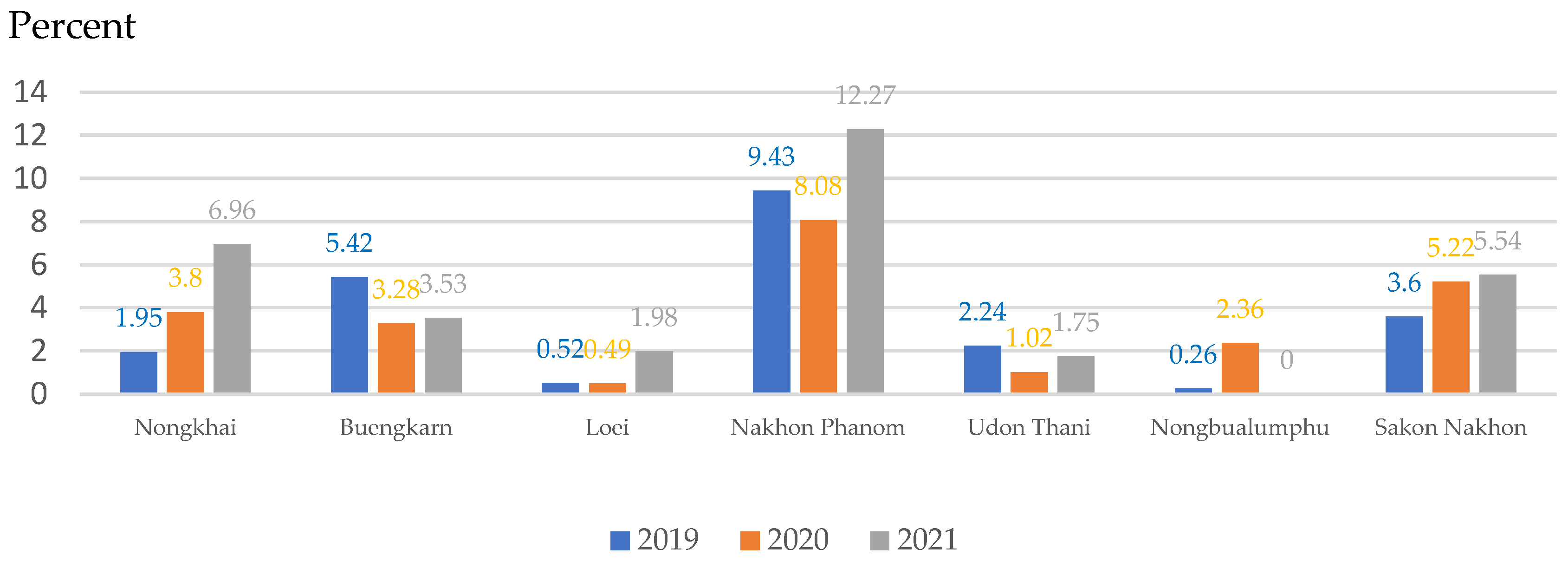
| Provinces | Number of People with Cholangiocarcinoma in 2019 | Number of People with Cholangiocarcinoma in 2020 |
|---|---|---|
| Nongkhai | 22 | 37 |
| Buengkarn | 8 | 7 |
| Loei | 54 | 84 |
| Nakhon Phanom | 7 | 10 |
| Udon Thani | 50 | 88 |
| Nongbualumphu | 19 | 12 |
| Sakon Nakhon | 161 | 130 |
| Sub-Basin | Y (% of OV) | X1 (lu) | X2 (soil) | X3 (road) | X4 (water) | X5 (stream) | X6 (temp) | X7 (ndmi) | X8 (ndvi) | X9 (savi) |
|---|---|---|---|---|---|---|---|---|---|---|
| Jomjaeng | 2.01 | 14.773 | 9.144 | 14.755 | 7.361 | 14.293 | 5.966 | −0.064 | 0.075 | 0.143 |
| Poopim | 1.05 | 49.947 | 33.838 | 47.748 | 29.494 | 43.984 | 7.954 | −0.060 | 0.115 | 0.218 |
| Phonnoi | 7.84 | 17.688 | 6.252 | 15.376 | 6.922 | 13.931 | 7.925 | −0.083 | 0.118 | 0.225 |
| Phonkaeyai | 0.84 | 14.279 | 11.576 | 14.489 | 6.149 | 15.661 | 8.210 | −0.081 | 0.124 | 0.237 |
| Wanplachuem-1 | 9.18 | 20.042 | 8.565 | 19.993 | 5.129 | 7.122 | 8.241 | 0.152 | 0.119 | 0.224 |
| Wanplachuem-2 | 6.48 | 60.884 | 24.128 | 64.132 | 14.349 | 61.311 | 7.593 | −0.037 | 0.104 | 0.199 |
| Klangmai | 4.38 | 37.048 | 24.577 | 37.011 | 5.862 | 32.838 | 7.677 | 0.042 | 0.117 | 0.227 |
| Nakaew | 2.52 | 60.758 | 29.858 | 74.811 | 40.229 | 59.603 | 7.740 | −0.035 | 0.116 | 0.224 |
| Nongphue | 1.95 | 80.795 | 34.581 | 90.847 | 18.963 | 79.482 | 7.909 | −0.049 | 0.119 | 0.227 |
| Maikrabok | 3.66 | 5.235 | 19.740 | 4.753 | 15.510 | 7.539 | 7.920 | −0.050 | 0.121 | 0.232 |
| Explanatory Variable Range Diagnostics | Training | Testing | Share | |||
|---|---|---|---|---|---|---|
| Minimum | Maximum | Minimum | Maximum | Training a | Testing b | |
| Model 1 distance to stream lines | 0.48 | 1055.51 | 133.04 | 610.29 | 1 | 0.45 * |
| Model 2 distance to stream lines | 0.48 | 1055.51 | 594.64 | 610.29 | 1 | 0.01 * |
| distance to water resource | 108.65 | 6054.45 | 970.21 | 1604.04 | 1 | 0.11 * |
| Model 3 distance to stream lines | 0.48 | 1055.51 | 195.81 | 527.24 | 1 | 0.31 * |
| distance to water resource | 108.65 | 6054.45 | 1319.44 | 1756.75 | 1 | 0.07 * |
| NDMI | −0.13 | 0.14 | 0.04 | 0.1 | 1 | 0.20 * |
| Model 4 distance to stream lines | 0.48 | 928.08 | 610.29 | 1055.51 | 0.88 * | 0.34 * |
| distance to water resource | 108.65 | 6054.45 | 1243.77 | 1604.04 | 1 | 0.06 * |
| NDMI | −0.13 | 0.1 | 0.07 | 0.14 | 0.85 * | 0.10 * |
| NDVI | 0.05 | 0.16 | 0.17 | 0.18 | 0.82 * | 0.00 * |
| Alternative OLS Models for OV-Predicted at the Watershed Level | Independent Variables | Coefficients | t-Stat | p-Value a | R2 |
|---|---|---|---|---|---|
| Y (%OV1) | Intercept | 0.465 | 4.373 *** | 0.000 *** | 0.524 |
| X8 (ndvi) | −1.534 | −0.878 n/s | 0.226 n/s | ||
| X9 (savi) | −6.032 | −2.212 n/s | 0.125 n/s | ||
| Y (%OV2) | Intercept | 4.528 | 1.975 *** | 0.000 *** | 0.672 |
| X7 (ndmi) | 1.125 | 0.769 *** | 0.044 *** | ||
| X8 (ndvi) | −3.116 | −0.890 *** | 0.023 *** | ||
| X9 (savi) | −9.852 | −2.326 n/s | 3.024 n/s | ||
| Y (%OV3) | Intercept | 62.042 | 3.031 *** | 0.000 *** | 0.713 |
| X5 (stream) | −5.047 | −2.068 *** | 0.048 *** | ||
| X7 (ndmi) | 4.246 | 1.875 *** | 0.034 *** | ||
| X8 (ndvi) | −9.874 | −2.661 *** | 0.021 *** | ||
| Y (%OV4) | Intercept | 57.410 | 0.979 *** | 0.000 *** | 0.681 |
| X5 (stream) | −0.0350 | −3.462 *** | 0.031 *** | ||
| X6 (temp) | 20.210 | 0.734 n/s | 1.263 n/s | ||
| X7 (ndmi) | 7.220 | 0.540 *** | 0.044 *** | ||
| X8 (ndvi) | −1524.360 | −0.548 *** | 0.026 *** | ||
| X9 (savi) | −2732.160 | −2.356 n/s | 0.895 n/s |
| Model Out-of-Bag Errors | Model 1 | Model 2 | Model 3 | Model 4 | ||||
|---|---|---|---|---|---|---|---|---|
| Number of Trees | 50 | 100 | 50 | 100 | 50 | 100 | 50 | 100 |
| MSE | 7.167 | 6.985 | 7.298 | 7.074 | 9.075 | 8.93 | 10.203 | 8.98 |
| % of variation explained | −3.432 | −1.358 | −5.511 | −2.267 | −33.117 | −31.003 | −46.689 | −29.111 |
| Top Variable Importance | Model 1 | Model 2 | Model 3 | Model 4 | ||||
|---|---|---|---|---|---|---|---|---|
| Variables | Importance | % | Importance | % | Importance | % | Importance | % |
| Distance to stream lines | 105.09 | 100 | 52.72 | 47 | 34.91 | 37 | 23.18 | 22 |
| Distance to water resource | 58.75 | 53 | 32.32 | 34 | 39.7 | 37 | ||
| NDMI | 27.89 | 29 | 20.32 | 19 | ||||
| NDVI | 22.79 | 22 | ||||||
| Training Data: Regression Diagnostics | Model 1 | Model 2 | Model 3 | Model 4 |
|---|---|---|---|---|
| R-Squared | 0.775 | 0.853 | 0.859 | 0.849 |
| p value | 0 | 0 | 0 | 0 |
| Standard Error | 0.053 | 0.06 | 0.043 | 0.051 |
| Y (% of OV) | X1 (Lu) | X2 (Soil) | X3 (Road) | X4 (Water) | X5 (Stream) | X6 (Temp) | X7 (Ndmi) | X8 (Ndvi) | X9 (Savi) | |
|---|---|---|---|---|---|---|---|---|---|---|
| Y (% of OV) | 1.000 | - | - | - | - | - | - | - | - | - |
| X1 | −0.167 | 1.000 | - | - | - | - | - | - | - | |
| X2 | −0.437 | 0.826 | 1.000 | - | - | - | - | - | - | - |
| X3 | −0.189 | 0.992 | 0.813 | 1.000 | - | - | - | - | - | - |
| X4 | −0.402 | 0.599 | 0.739 | 0.635 | 1.000 | - | - | - | - | - |
| X5 | −0.226 | 0.985 | 0.838 | 0.984 | 0.612 | 1.000 | - | - | - | - |
| X6 | 0.173 | 0.116 | 0.184 | 0.106 | 0.109 | 0.067 | 1.000 | - | - | - |
| X7 | 0.395 | 0.060 | −0.143 | −0.061 | −0.258 | −0.193 | 0.243 | 1.000 | - | - |
| X8 | 0.082 | 0.092 | 0.227 | 0.095 | 0.134 | 0.062 | 0.969 | 0.171 | 1.000 | - |
| X9 | 0.079 | 0.097 | 0.242 | 0.103 | 0.144 | 0.074 | 0.950 | 0.150 | 0.997 | 1.000 |
Disclaimer/Publisher’s Note: The statements, opinions and data contained in all publications are solely those of the individual author(s) and contributor(s) and not of MDPI and/or the editor(s). MDPI and/or the editor(s) disclaim responsibility for any injury to people or property resulting from any ideas, methods, instructions or products referred to in the content. |
© 2023 by the authors. Licensee MDPI, Basel, Switzerland. This article is an open access article distributed under the terms and conditions of the Creative Commons Attribution (CC BY) license (https://creativecommons.org/licenses/by/4.0/).
Share and Cite
Pumhirunroj, B.; Littidej, P.; Boonmars, T.; Bootyothee, K.; Artchayasawat, A.; Khamphilung, P.; Slack, D. Machine-Learning-Based Forest Classification and Regression (FCR) for Spatial Prediction of Liver Fluke Opisthorchis viverrini (OV) Infection in Small Sub-Watersheds. ISPRS Int. J. Geo-Inf. 2023, 12, 503. https://doi.org/10.3390/ijgi12120503
Pumhirunroj B, Littidej P, Boonmars T, Bootyothee K, Artchayasawat A, Khamphilung P, Slack D. Machine-Learning-Based Forest Classification and Regression (FCR) for Spatial Prediction of Liver Fluke Opisthorchis viverrini (OV) Infection in Small Sub-Watersheds. ISPRS International Journal of Geo-Information. 2023; 12(12):503. https://doi.org/10.3390/ijgi12120503
Chicago/Turabian StylePumhirunroj, Benjamabhorn, Patiwat Littidej, Thidarut Boonmars, Kanokwan Bootyothee, Atchara Artchayasawat, Phusit Khamphilung, and Donald Slack. 2023. "Machine-Learning-Based Forest Classification and Regression (FCR) for Spatial Prediction of Liver Fluke Opisthorchis viverrini (OV) Infection in Small Sub-Watersheds" ISPRS International Journal of Geo-Information 12, no. 12: 503. https://doi.org/10.3390/ijgi12120503