A High-Resolution Spatial Distribution-Based Integration Machine Learning Algorithm for Urban Fire Risk Assessment: A Case Study in Chengdu, China

Abstract

The development and functional perfection of urban areas have led to increasingly severe fire risks in recent decades. Previous urban fire risk assessment methods relied on subjective judgment, rough data collection, simple linear statistical methods, etc. These drawbacks can lead to low robustness of evaluation and inadequate generalization ability. To resolve these problems, this paper selects the indicator and regression models based on the high-resolution data of the spatial distribution characteristics of Longquanyi distinct in Chengdu, China. and proposes an integrated machine learning algorithm for fire risk assessment. Firstly, the kernel density analysis is used to map the fourteen urban characteristics related to fire risks. The contributions of these indicators (characteristics) to fire risk and its corresponding index are determined by Random Forest (RF), Gradient Boosting Decision Tree (GBDT), and eXtreme Gradient Boosting (XGBoost). Then, the spatial correlation of fire risks is determined through Moran’s I, and the spatial distribution pattern of indicator weights is clarified through the raster coefficient space analysis. Finally, with these selected indicators, we test the regression performance with a backpropagation neural network (BPNN) algorithm and a geographically weighted regression (GWR) model. The results indicate that numerical variables are more suitable than dummy variables for estimating micro-scale fire risks. The main factors with a high contribution are all numerical variables, including roads, gas pipelines, GDP, hazardous chemical enterprises, petrol and charging stations, cultural heritage protection units, assembly occupancies, and high-rise buildings. The machine learning algorithm integrating RF and BPNN shows the best performance (R² = 0.97), followed by the RF-GWR integrated algorithm (R² = 0.87). Compared with previous methods, this algorithm reduces the subjectivity of the traditional assessment models and shows the ability to automatically obtain the key indicators of urban fire risks. Hence, this new approach provides us with a more robust tool for assessing the future fire safety level in urban areas.

1. Introduction

Fire is a common phenomenon in the world today. Rapid urbanization can increase the number of factors contributing to urban fire risks and increase the difficulty of fire prevention and control. For example, about 748 thousand fires in 2021 were reported in China, with 1987 deaths, 2225 injuries, and more than 6.75 billion yuan in direct property losses [1]. Such threats are severe in crowded places, such as business districts and residential communities, making it necessary to assess and control the fire risks and improve urban fire safety.

Nowadays, fire risk assessment studies in urban areas often focus on identifying key factors and assessment models. The shortcomings of existing research are mainly reflected in the levels of data collection, indicator selection, and model selection.

At the data level, the resolution of datasets has a major impact on the fire risk assessment results. The minimum units of most urban fire studies are buildings [2,3,4,5], blocks [6,7], and grids with dimensions of several kilometers [8,9]. The relationship between urban fire dynamics and urban growth varied at different spatial scales as well as across space [10]. Different sizes of grids may have completely different solutions in spatial optimization models [11]. A low-resolution dataset means a large grid size in the study area, which can lower the accuracy of fire risk prediction and fail to represent the spatial heterogeneity of fire risk distribution. For example, Jin et al. [12] divided San Francisco into 100 grids to explore the spatiotemporal dynamics of fire situations. The low resolution of the grid leads to imprecise assessment results that only reflect the fire situation at a macro level. On the other hand, high-resolution data can help improve the accuracy of the model; however, it often poses challenges to data collection. Therefore, many studies only focus on fire accidents [13,14], instead of the primary driving factors of fire risks.

At the indicator level, the complexity of fire risks makes it difficult to build a risk assessment index with strong theoretical support. Fire risks are not only affected by social, economic, and demographic factors [15] they are also related to the ability of communities and buildings to withstand fire incidents, residential characteristics, and human behaviors [16,17]. Prior studies explain the association between fire risks and their factors and provide some insight into the analysis of uncertain events [18,19,20,21]. However, they tend to ignore the relationship between the spatial distribution of fire risks and the high-resolution spatial layout of urban areas [22]. The spatial distribution of fire risk in urban areas can be explained by the characteristics of urban functional layout, including residential districts, business districts, storage districts, road networks, petrol stations, and so on. These characteristics can help predict human activities, and the areas where human activities converge often have high rates of fires. For example, the number of fires in residential and commercial districts is usually higher than that in storage areas or parks.

At the model level, aleatoric, epistemic, and operational uncertainties are the main challenges for fire risk assessment and prediction. To address these uncertainties and improve the accuracy of fire prediction, several studies [23,24,25] have attempted to use non-parametric models represented by machine learning methods. In addition, McCarty et al., Kumar et al., and Chen et al. apply the spatial econometric models to explore the spatial correlations between different data points and between the spatial distributions of fire risks [16,26,27]. However, these studies suffer from problems as they analyze the entire fire dataset and the values of related variables, which only allow for the evaluation of the impact of factors on fire risk across the entire study area without detecting and characterizing the spatial variations in the impact of factors on fire risk at the local level, leading to biased assessment results.

With the increasing demand for objective and real-time risk assessments in the industrial sector, the use of machine learning algorithms in academia has also become a trend [28]. Machine learning can automatically analyze data to extract patterns and utilize these patterns for predicting unknown data. Neural networks, as a type of non-parametric machine learning algorithm, can help avoid issues such as biases and oversimplification that arise from inaccurate assumptions. As one of the most versatile and accurate models among neural network methods, the backpropagation neural network (BPNN) has better generalization performance and more robust model predictions [29]. Hence, it has become a popular method in natural disaster assessment [30], security risk assessment [31], financial risk assessment [32,33], and environmental management [34]. Despite the widespread application of BPNN in assessing and predicting risks, this method is still absent in studying the relationship between fire risks and urban fire-related factors at the grid level. The non-parametric nature of BPNN, along with its ability to comprehend complex systems and their correlations, offers advantages in fitting fire risk models and contributes to providing new ideas in fire risk modeling.

In terms of the spatial analysis of fire risks, the relationship between fire risk factors varies with geographic locations. Therefore, we need to consider spatial non-stationarity, which is the variability in the relationship or structure among variables due to changes in geographic locations. Geographically Weighted Regression (GWR) can effectively capture the effects of spatial heterogeneity and detect non-smooth spatial relationships and regional variations as a supportive tool, along with other sets of information, such as the local weights of independent variables [35]. The applications of neural network models to studying local spatial heterogeneity remain an open research area. Accordingly, we attempt to use GWR to overcome limitations such as spatial relation analysis of neural networks in this aspect.

In recent years, geographic information systems (GIS) and spatial statistics have become important tools in fire risk assessment and analysis. These tools enable the manipulation of large volumes of data and promote the development of complex models and statistical algorithms [36]. Particularly, territorial spatial planning provides a guide for the development of urban space. The results of the grid-scale fire risk assessment can guide urban fire planning by combining land use development and socioeconomic demographic data from territorial spatial planning. The geographical characteristics of the territory are fundamental to performing good urban safety management; in particular, land cover maps are crucial to defining sustainable management and planning policies [37,38]. This combination can further match fire infrastructure construction with urban development and promote the future public safety development of the region.

In summary, it is important to utilize high-resolution data to identify the key fire risk indicators related to urban characteristics. In this study, machine learning methods were used to analyze the influence of urban functional layout on the spatial distribution of fire risk, explore the spatial correlation of fire risk at a micro-scale, and examine the spatial heterogeneity of indicators influencing fire risk. The suitability of BPNN and GWR models for fire risk assessment in urban areas was compared. The research data were obtained from urban land spatial planning data, and the assessment results of fire risk are closely related to urban development. This research contributes to guiding urban regional fire protection planning, further optimizing the overall layout of urban safety, ensuring that regional public fire protection infrastructure construction matches urban development, and ensuring that the distribution of fire rescue forces aligns with the regional development level, thus ensuring the high-quality social and economic development of the urban region in the future.

The following sections of this paper are constructed as follows: Section 2 presents the materials and methods, including this study area, urban spatial distribution characteristics, fire dataset, and methods. We then report the main results of the indicator selection in Section 3.1, the indicator multicollinearity test in Section 3.2, the spatial patterns of indicators and fire risks in Section 3.3, and the comparison between BPNN and GWR fire risk assessment models in Section 3.4. Following them, Section 4 is the discussion of results and relative studies. Conclusions and outlook are presented in Section 5.

2. Materials and Methods

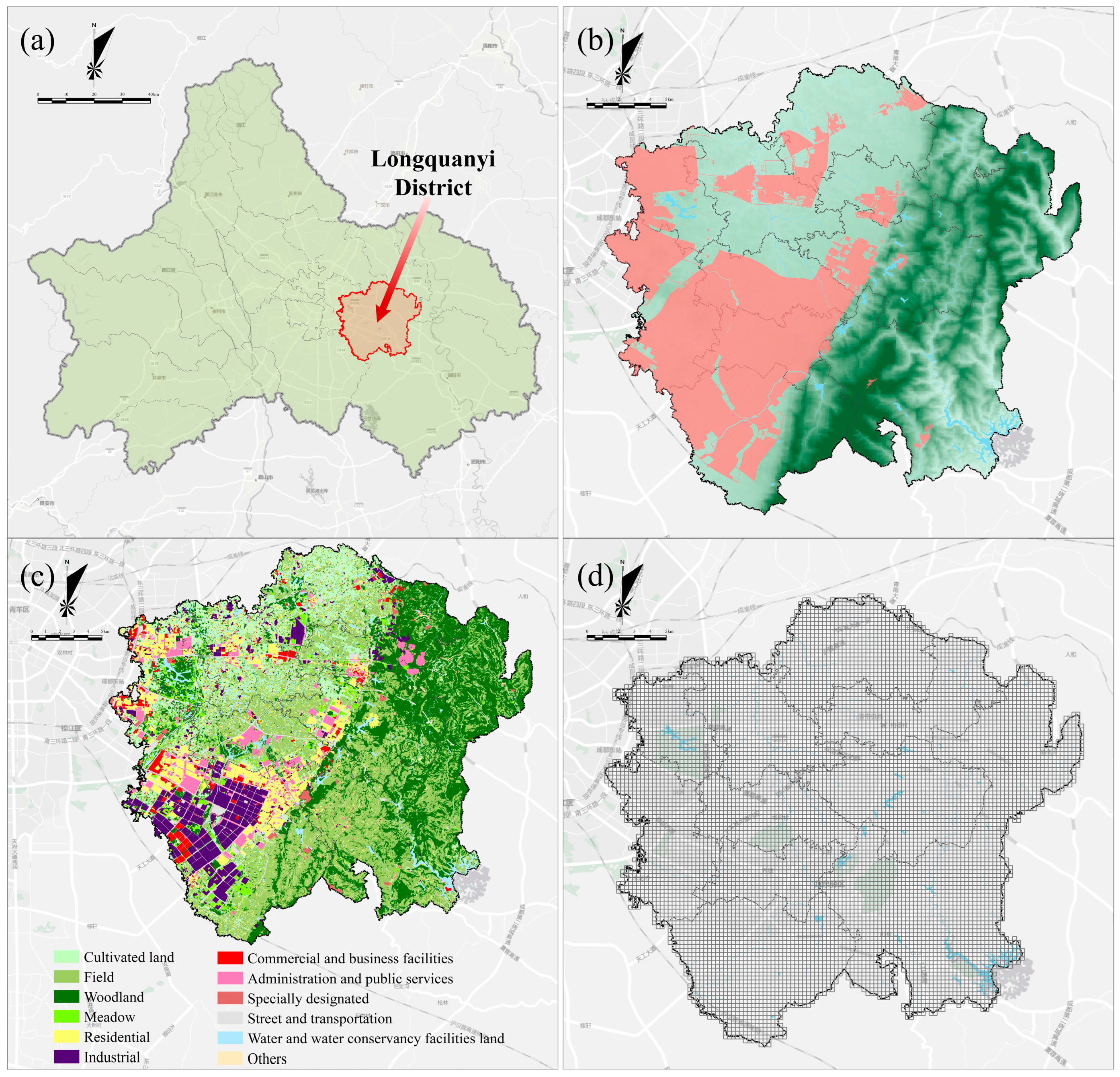
2.1. Study Area

This study area is an administrative district named Longquanyi in the eastern part of Chengdu City, Sichuan Province, as shown in Figure 1a. It is between 30°27′52″–30°43′23″ north latitude and 104°08′19″–104°27′09″ east longitude. The topography of the central city is flat, except for a very few areas in the east, which are located in the shallow hills. The rest of the area belongs to the flat dam area of the Chengdu Plain, with a slight natural slope, and the pink area is the town development area, as shown in Figure 1b. The land survey data provided by the Longquanyi District Bureau of Natural Resources and Planning includes commercial and business facilities, administration and public services, specially designated streets and transportation, water and water conservancy facilities, land, cultivated land, fields, wooded land, meadows, residential, industrial, and others with a 1 m resolution. The central city of Longquanyi District has 168.71 km², including 83.76 km² of urban construction land, 21.20 km² of residential land, 8.25 km² of land for public administration and public services, 5.11 km² of commercial services, 28.43 km² of industrial land, 3.28 km² of storage land, 11.58 km² of transportation land, 0.79 km² of land for public facilities, and 5.12 km² of land for green space and open space, as shown in Figure 1c. To facilitate the subsequent geometry calculation in the projection space, the China Geodetic Coordinate System 2000 is used to determine the geographic coordinates of the fire data. Considering the size of the Longquanyi District and the data set, this study area is transformed into a grid space with a resolution of 250 m × 250 m. The processed dependent and independent variable data are mapped to the corresponding grids in the subsequent study to build models for indicator analysis and fire risk assessment. This study area after gridding is shown in Figure 1d.

2.2. Urban Spatial Distribution Characteristics

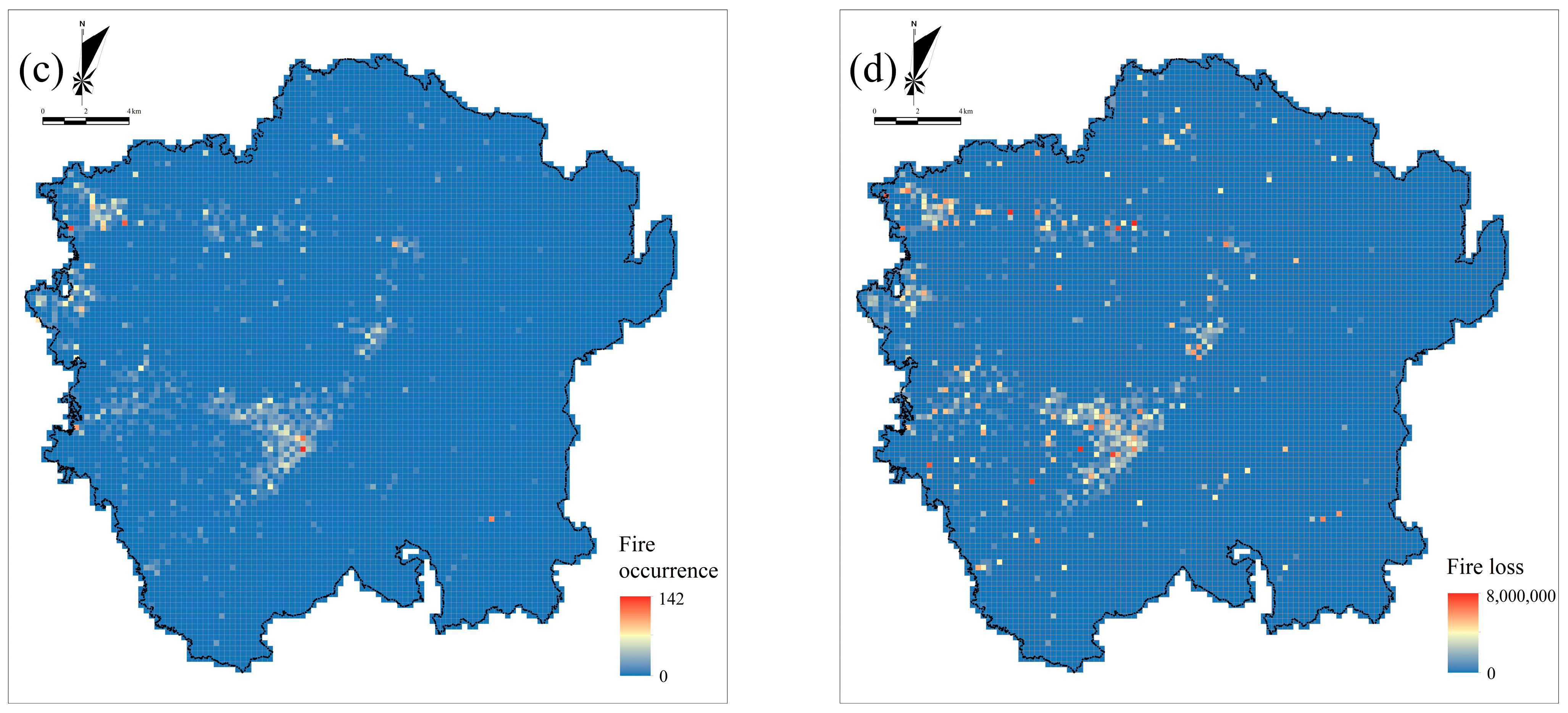
As a subordinate part of territorial spatial planning, fire safety planning needs to consider the factors of regional spatial patterns, functional zoning, infrastructure, and land use layout. Therefore, urban spatial distribution characteristics, including the above aspects, were used to study fire risk in this study, with a total of 14 characteristics. These indicators were collected through the comprehensive application of web crawling and multi-source data from many departments. The details of each indicator, including name, data source, abbreviation, unit, and value, were listed in

Table 1. Fire risk indicators and data sources.

Indicator	Data Sources	Abbreviation	Unit	Value
Road	https://www.openstreetmap.org/ (accessed on 14 July 2022)	ROAD	km/km2	Numerical
Gas pipeline	Bureau of Economy and Information Technology	PIPE	km/km2	Numerical
GDP	Resource and Environment Science and Data Center	GDP	1/km2	Numerical
Population	https://hub.worldpop.org/geodata/summary?id=49730 (accessed on 14 July 2022)	POPU	1/km2	Numerical
Hazardous chemical enterprises	Fire and Rescue Administration	HAZA	1/km2	Numerical
Petrol and charging stations	Amap	PETR	1/km2	Numerical
Cultural Heritage Protection Unit	Bureau of Culture, Sports and Tourism	HERI	1/km2	Numerical
Assembly occupancies 1	Amap	ASSE	1/km2	Numerical
High-rise building	Fire and Rescue Administration	HIGH	1/km2	Numerical
Commercial service zone	Bureau of Natural Resources and Planning	COMM	—	Binary
Industrial zone	Bureau of Natural Resources and Planning	INDU	—	Binary
Warehouse zone	Bureau of Natural Resources and Planning	WARE	—	Binary
Residential zone	Bureau of Natural Resources and Planning	RESI	—	Binary
Land development intensity	Bureau of Natural Resources and Planning	LAND	—	Binary

¹ Assembly occupancies mainly mean business halls, malls, auditoriums, cinemas, theaters, and stadiums, etc., which are large and gather a large number of people simultaneously.

. When analyzing the key influencing factors of fire risk, kernel density processing is performed, and the optimal bandwidth is calculated by an adaptive method. The data are displayed in ArcGIS software with graded symbolic color to show the spatial distribution of each indicator, as shown in Figure 2.

As shown in Table 1, numerical variables are represented by consecutive numbers, while dummy variables are marked with “0” or “1”. Take the indicator “land” as an example; the grid within the urban development boundary is characterized as value 1, and the grid outside the urban development boundary is assigned value 0. Resampling was performed when the resolution of the original data set was greater than 250 m × 250 m.

2.3. Fire Dataset

The historical fire data were collected in Longquanyi District from 2010 to 2021 and provided by the Chengdu Longquanyi fire protection and rescue guards. The data contains aspects of fire date, cause of fires, locations, direct property losses, and response times. The fire data for this decade is 2096 fires, with a direct economic loss of 40,189,000 RMB.

Modeling fire risk in urban areas is theoretically complex. Many scholars have defined and modeled fire risk from different perspectives [39]. Yoe [40] holds the view that risk is a measure of the probability and consequence of uncertain future events; it has two important components: an undesirable consequence and the probability it will occur. The most common definition of fire risk takes into account both the probability of occurrence and the consequences of an event [36,41]. In this paper, we adopted this definition of risk. The fire risk is characterized as shown in Equation (1):

$$R=P·L$$

(1)

where R means the fire risk; P is the fire occurrence probability, characterized as the fire density of the grid; and L represents the undesirable consequence, characterized as the direct economic loss from the fire of the grid.

To prevent uncertainties and errors in the fire record, kernel density analysis is applied to process fire occurrence and fire loss. In the process of kernel density analysis, the size of the bandwidth is mainly related to the analysis scale and geographic phenomena. A smaller bandwidth can result in more high- or low-value areas in the density distribution, while a larger bandwidth can make hotspots more prominent at the global scale. In addition, the setting of bandwidth is also related to the dispersion of data points. Sparse data points are suitable for using a larger bandwidth, while for dense data points, a smaller bandwidth should be considered. In this study, the bandwidth is calculated by the “Silverman rule of thumb”, a bandwidth estimation method based on empirical rules that was first proposed in 1986 by Silverman [42]. and the relevant data are extracted into corresponding spatial grids, as shown in Figure 3.

2.4. Methods

2.4.1. Indicator Selection Models

Considering the characteristics of complex nonlinear relationships among fire risk factors, we selected RF, GBDT, and XGBoost algorithms to investigate the relationship between urban characteristics and fire risk distribution patterns. RF is a highly flexible supervised machine learning algorithm based on the idea of Bagging, which introduces random features based on Bagging to improve the independence between each base model further. To reveal the nonparametric characteristics of complex systems and their correlations, studies comparing RF with multiple regression models show that RF performs better [43,44,45]. GBDT is a classical algorithm of Boosting, and the basic idea is to sum the results of all weak classifiers to obtain the predicted value and residuals. Then, through multiple iterations, the residuals generated by the training process are continuously reduced to classify or regress the data [46]. XGBoost is an improved algorithm for boosting based on GBDT. Compared to GBDT, XGBoost adds a regular term to the objective function for controlling the complexity of the model and adds a parameter to each subtree so that the weight of each subtree is reduced to prevent overfitting.

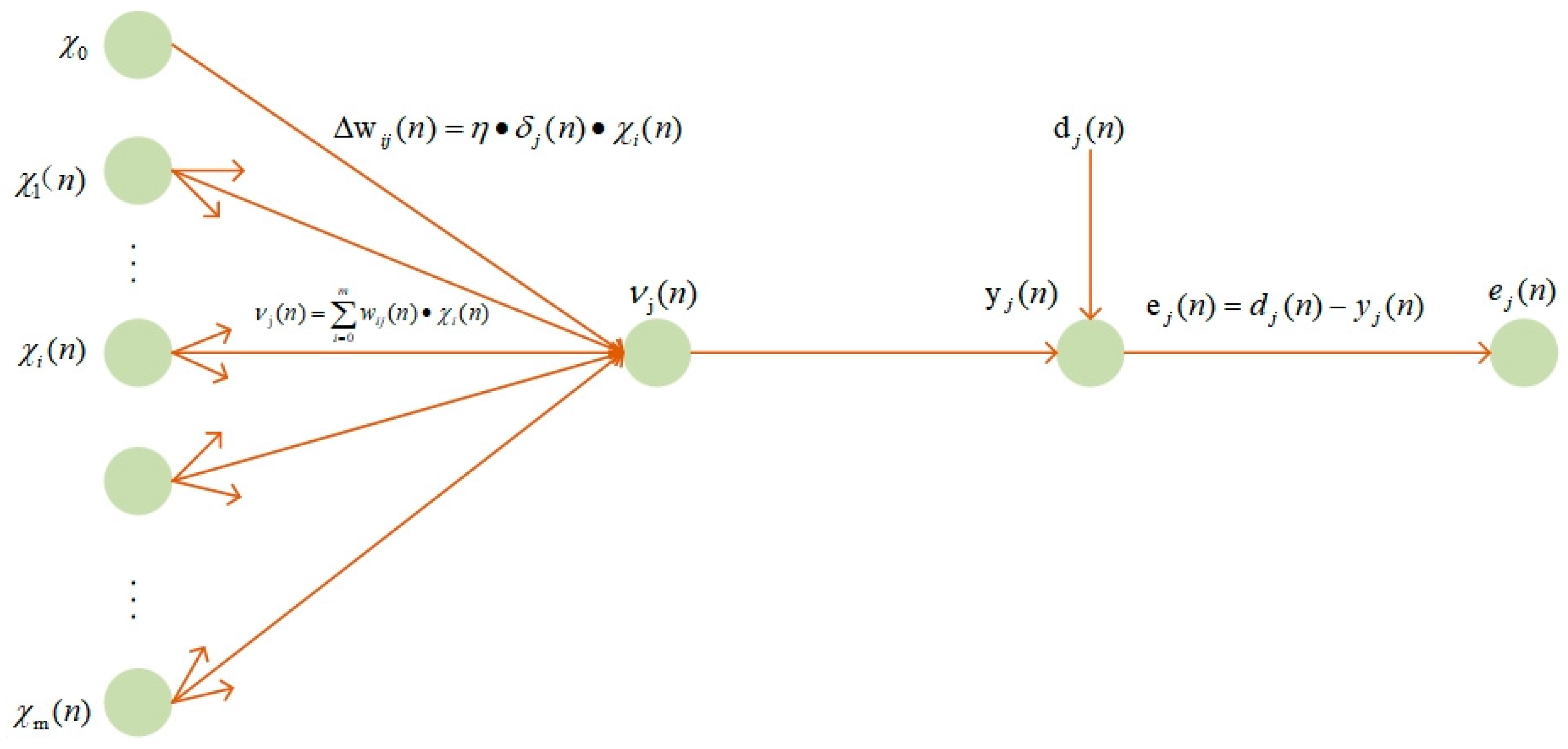
2.4.2. Fire Risk Assessment Models

In this study, two types of models were selected to model fire risk: BPNN and GWR. A typical BPNN structure consists of three layers, which are the input layer, hidden layer, and output layer, as shown in Figure 4. The network connection weights are corrected based on the error between the actual output and the expected output. Finally, the neural network error is smaller than the target function to achieve the expected result. This study uses the fire risk indicator as input and the fire risk as output.

The modified value $\Delta w_{ji}(n)$ of the synaptic weights is defined according to Equation (2):

$$\Delta w_{ji}(n)=\eta ·{\delta }_j(n)·x_i(n)$$

(2)

where: $\eta$ is error backpropagation learning rate, ${\delta }_j(n)$ is local gradient, and $x_i(n)$ is input signal of $i$ neurons.

The ${\delta }_j(n)$ specifies the required change value in synaptic weights, and its mathematical expression is as follows:

$${\delta }_j(n)=e_j(n)·f^{\prime }(v_j(n))$$

(3)

the expression for $e_j(n)$ is shown in Equation (4):

$$e_j(n)=d_j(n)-y_j(n)$$

(4)

$d_j(n)$ refers to the desired output. $f(x)$ is an activation function. The widely used activation functions include the threshold, segmentation, Sigmoid, and tanh functions. Since the Sigmoid function allows for the modeling of non-linear relationships, this study chose the Sigmoid function as the activation function $v_j(n)$ is the input of neuron j. Its expression is Equation (5):

$$v_j(n)={\displaystyle \sum _{i=0}^m{w}_{ji}(n)·x_i(n)}$$

(5)

$w_{ji}(n)$ characterizes the weight of $x_i(n)$.

In neural networks, hidden layers are needed when the data are nonlinearly separated. However, the data set collected in this study is small, and the fire risk features are not complex. Therefore, one hidden layer is selected, and the network structure has three layers. The range of neurons in the hidden layer and other optimal parameters of the network model are determined by tuning hyperparameters, and the parameters are set as shown in

Table 2. BPNN parameter settings.

Parameter	Parameter Tuning	Optimal Setting
Activation functions	Logsig, tansig, ReLU	tansig
Transfer functions	Logsig, tansig, purelin	purelin
Number of neurons in hidden layer	[4, 20]	19
Training functions	Traingd, traingdm, traingda, traingdx, trainrp, traincgb, trainscg, trainlm	traincgb
Learning Rate	0.05, 0.06, 0.07, 0.08, 0.09, 0.1	0.05
Momentum parameters	0.5, 0.6, 0.7, 0.8, 0.9	0.9

.

From the MSE and R, the optimal number of hidden layer neurons is 19, as shown in Figure 5a. At this point, the model has the maximum R and the minimum MSE. After inputting the optimal parameters in Table 2, the distribution of the error values of the BPNN model is shown in Figure 5b. It can be seen that the errors of the BPNN model after tuning the parameters are minor and concentrated between [−0.01, 0.01]. The errors satisfy the accuracy requirements of the model training.

Spatial non-stationarity is commonly found in spatial data. To effectively reflect the spatial non-stationarity of characteristics in regression relationships, spatial variable parameter models are proposed, where the regression parameters of the model are functions concerning geographic location [48]. The GWR model is proposed based on local regression analysis and variable parameter studies [49]. The relationship between the dependent variable and independent variables can be modeled locally for each location by GWR; therefore, it can explain the variability of the effects of different fire risk indicators on fire risk at different locations. Specifically, the GWR model can be interpreted as follows: in a spatial region, a continuous decay function is calculated based on the spatial distance of the element locations, and this decay function is brought in, and the weight of each element in the local regression equation is calculated to obtain the weighted regression equation. The model is defined in Equation (6):

$$Y_i={\beta }_0(u_i,v_i)+{\displaystyle \sum _{j=1}^p{\beta }_j(u_i,v_i)·X_{ij}+{\epsilon }_i}\begin{array}{cc}& i=1,2,\dots ,n\end{array}$$

(6)

A given coordinate $(u_i,v_i)$, ${\beta }_j(u_i,v_i)$ can be estimated using locally weighted least squares, as in Equation (7):

$$\min {\displaystyle \sum _{i=1}^n{\left[y_i-{\displaystyle \sum _{j=1}^p{\beta }_j(u_i,v_i)·x_{ij}}\right]}^2}·w_j(u_i,v_i)$$

(7)

where $w_j(u_i,v_i)$ is the spatial weight at a coordinate $(u_i,v_i)$.

Let $\beta (u_i,v_i)={\left\{{\beta }_0(u_i,v_i),{\beta }_1(u_i,v_i),\dots ,{\beta }_p(u_i,v_i)\right\}}^T$, then the decay function is shown as Equation (8):

$$\widehat{\beta }(u_i,v_i)={\left\{X^{T}W(u_i,v_i)X\right\}}^{-1}·X^{T}W(u_i,v_i)Y$$

(8)

where, $X=\left[\begin{array}{cccc}1& x_{11}& \dots & x_{1p}\\ 1& x_{21}& \dots & x_{2p}\\ \dots & \dots & \dots & \dots \\ 1& x_{n1}& \dots & x_{np}\end{array}\right]\begin{array}{cc}, & Y\end{array}=\left[\begin{array}{c}{y}_1\\ y_2\\ \dots \\ y_n\end{array}\right]$.

The spatial weight matrix is $W(u_i,v_i)=\left[\begin{array}{cccc}{w}_{i1}& 0& \dots & 0\\ 0& w_{i2}& \dots & 0\\ \dots & \dots & \dots & \dots \\ 0& 0& \dots & w_{in}\end{array}\right]$.

The most widely used Gaussian kernel function is used in this study, and its form is shown in Equation (9) [50]. The smaller $d_{ij}$, the greater the weight between the two points. $b$ is the bandwidth, which controls the rate at which the weights fall. The larger the bandwidth, the slower the weights decay with increasing distance. The smaller the bandwidth, the faster the weights decay with increasing distance.

$$w_{ij}=\exp \left\{-{(\frac{d_{ij}}{b})}^2\right\}$$

(9)

As can be seen from the parameters of the spatial weight function, the choice of bandwidth is a critical factor in constructing the spatial weight matrix. The commonly used criteria for optimal bandwidth selection are the Cross-validation criterion, Generalized cross-validation criterion, and Corrected Akaike information criterion (AIC). The AIC criterion is modified based on the significant likelihood by considering the number of independent parameters and improving the fit quality by increasing the free parameters, thus avoiding over-fitting [51]. With this approach, a model can best explain the data but contain a minimum number of free parameters. Since the AIC method considers model complexity and accuracy, the bandwidth corresponding to the geographically weighted regression weight function with the smallest AIC value is chosen for this study.

Before modeling spatial data, one should determine whether spatial correlation or heterogeneity exists in the data. If the effect of fire risk indicators on fire risk is consistent over space, then a global regression model can be used. Global estimates can mask geographic phenomena if there is a lack of consistency in the spatial impact of the indicators on fire risk. Suppose the characteristics of the data need to be understood, and an inappropriate model is used to analyze the problem. In that case, it may lead to a poor model fit and failure to obtain realistic results. Generally speaking, Moran’s index is used to measure spatial correlation. It is based on the principle that the product of attributes and spatial relationships expresses spatial correlation. Moran’s index value represents the distribution of an attribute value over the whole space, reflecting the spatial dependence of the observed value over the whole spatial range. The formula for it is as follows [52,53]:

$$I=\frac{n}{S_0}=\frac{{\displaystyle \sum _{i=1}^n{\displaystyle \sum _{j=1}^n{w}_{ij}·z_i·z_j}}}{{\displaystyle \sum _{i=1}^n{z}_i^2}}$$

(10)

where $z_i$ is the deviation of the attributes of the element $i$ from the mean, denoted as $z_i=(x-\stackrel{⌢}{x})$. $S_0$ is the set of all spatial weights, denoted as Equation (11):

$$S_0={\displaystyle \sum _{i=1}^n{\displaystyle \sum _{j=1}^n{w}_{ij}}}$$

(11)

From the calculation of Moran’s index, it is known that when the values of two elements are greater than or less than the mean at the same time, the product of deviations is positive, and 0 < I < 1 indicates aggregation. When the values of two elements differ in size from the mean value, the product of deviations is negative, and −1 < I < 0 indicates dispersion. When the positive and negative values of the deviation cancel each other out, the I value is closer to 0, the closer the distribution is to random. The larger the deviation, the larger the absolute value of the result obtained. It indicates a more significant spatial aggregation or dispersion relationship.

The calculation of the local Moran index is shown in Equation (12):

$$I_i=\frac{y_i-\overline{y}}{S^2}{\displaystyle \sum _{j\ne i}^n{w}_{ij}(y_i-\overline{y})}$$

(12)

where I_i is the local Moran index of the $i$th grid, $S^2$ is $\frac{1}{n}{{\displaystyle \sum (y_i-\overline{y})}}^2$, $w_{ij}$ is the spatial weight, and $n$ is the number of all grids.

3. Results

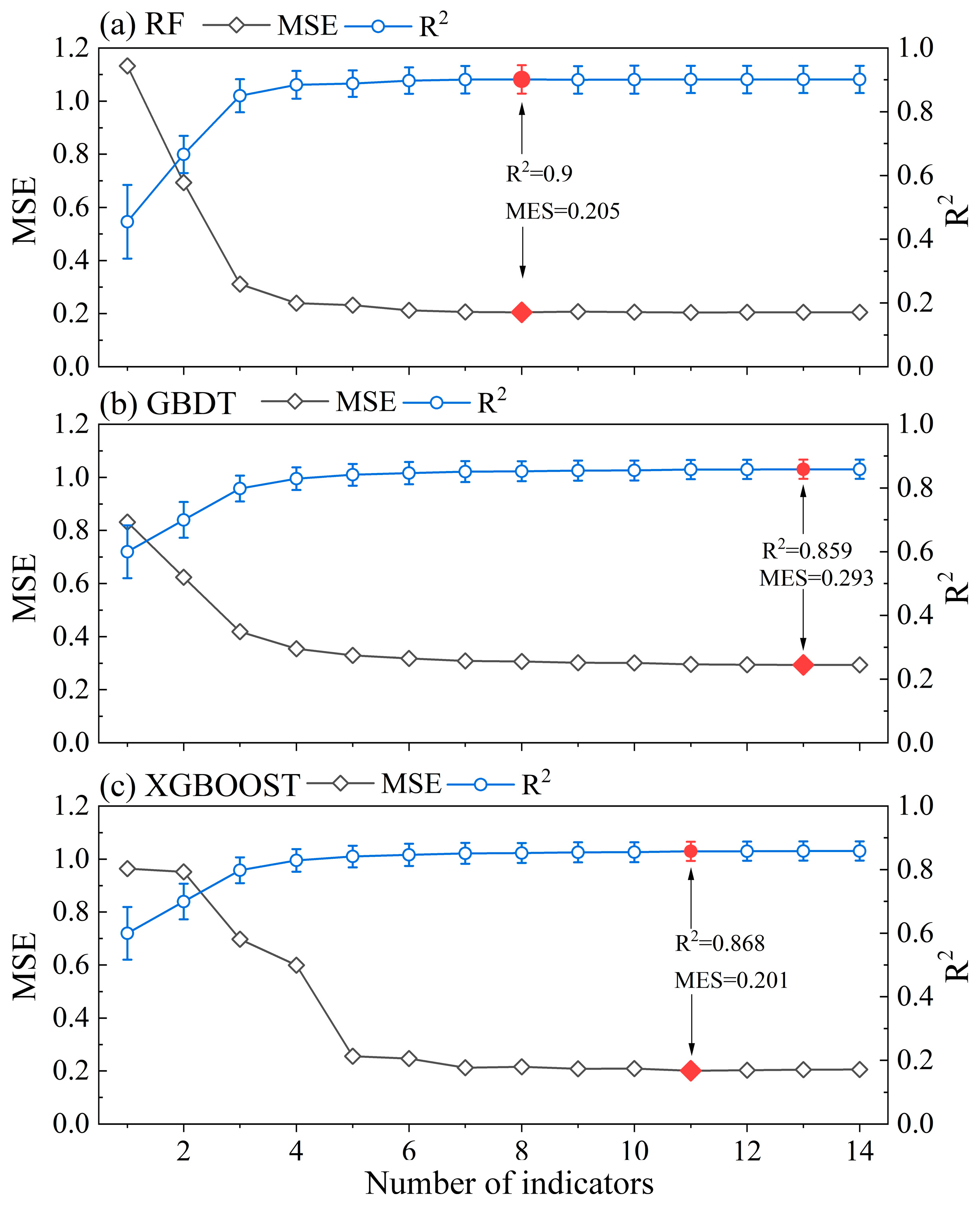
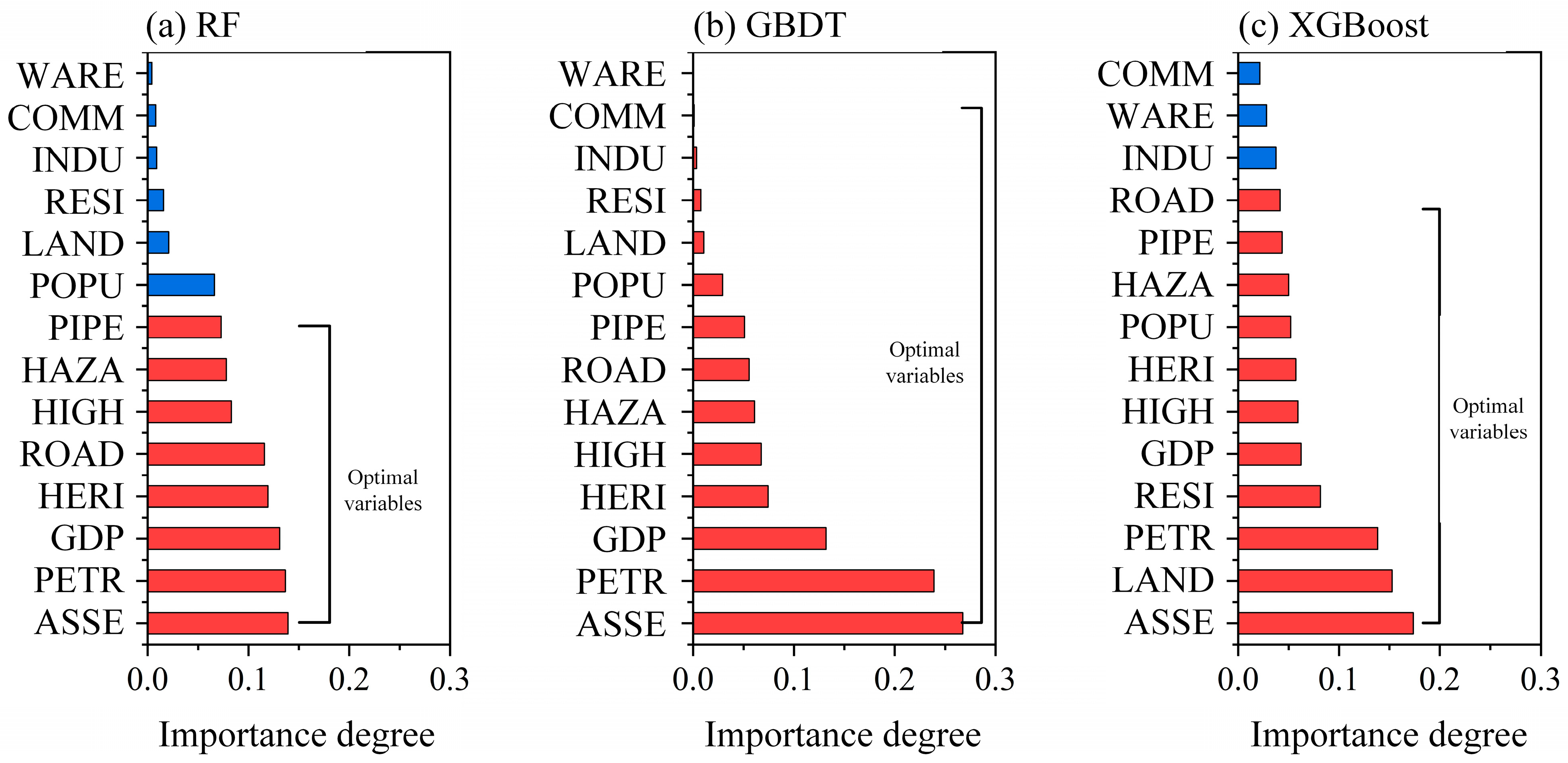
3.1. Indicator Selection

Five-fold cross-validation with five repetitions is used to compare the average performance of different models after training. In order to test which model has the best performance, the MSE and the coefficient of determination R² are used as criteria for variable screening. The changes in the optimal subset of independent variables selected based on the characteristic variables are shown in Figure 6. The blue line with the error bar means the indicators’ coefficient of determination, R². The black lines mean the MSE. The optimal number of indicators obtained from each model simulation is marked with a red dot.

One observation from Figure 6 is that RF exhibits the best performance, selecting eight indicators with 0.9 R² and 0.205 MSE. Then, followed the XGBoost method. It selects eleven indicators with 0.868 R² and 0.201 MSE. Finally, thirteen indicators were selected by the GBDT method, with 0.859 R² and 0.293 MSE.

The importance of each indicator and the optimal feature variables selected based on the feature variables are shown in Figure 7. To facilitate identification and analysis, all the indicators were listed in ascending order of importance. Meanwhile, the selected indicator is marked out with a red column; otherwise, it is marked out with a blue column.

Noticeably, PIPE, HAZA, HIGH, ROAD, HERI, GDP, PETR, and ASSE were the selected indicators by RF. In the following study, we will conduct a regression analysis based on these eight indicators. Another observation from Figure 7 is that the common indicators selected from the three models, including ASSE, PETR, GDP, HERI, ROAD, HIGH, HAZA, and PIPE, are all numerical variables, which indicates that numerical variables are more representative than dummy variables in estimating fire risk.

3.2. Indicators Multicollinearity Test

The problem of multicollinearity among explanatory variables can interfere with the significance of the variables. Therefore, before conducting regression, it is necessary to check the multicollinearity among the independent variables. In linear regression models, the variance inflation factor (VIF) is commonly used as a measure of multicollinearity. Generally speaking, when VIF < 10, there is no multicollinearity among the variables. A VIF between 10 and 100 indicates strong multicollinearity among the variables. And there is severe multicollinearity among the variables in the conditional VIF ≥ 100. The results of VIF, which measures multicollinearity, are presented in

Table 3. Results of multiple covariance test for fire risk indicators.

Indicator	VIF	Indicator	VIF
ROAD	1.56	HIGH	1.9
PIPE	2.87	HERI	1.19
GDP	1.2	PETR	2.77
ASSE	2.61	HAZA	1.18

. The value of VIF among the selected variables is all less than 3, which indicates that there is no multicollinearity among the selected independent variables and proves the indicators selected by RF are reasonable.

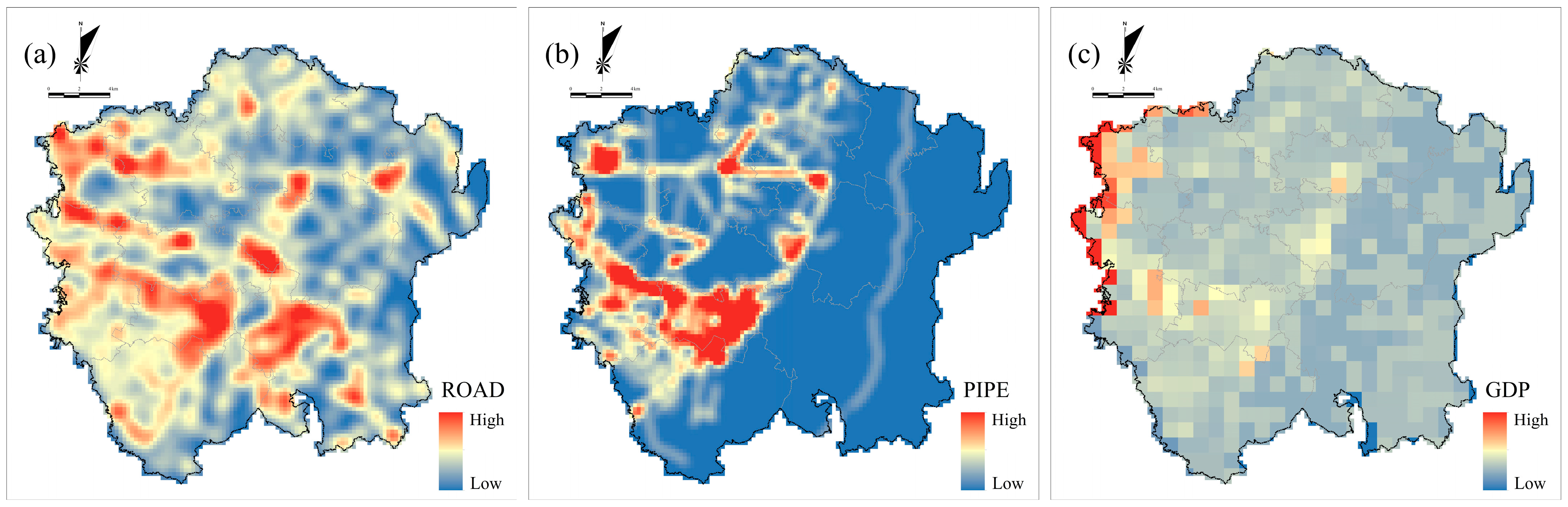
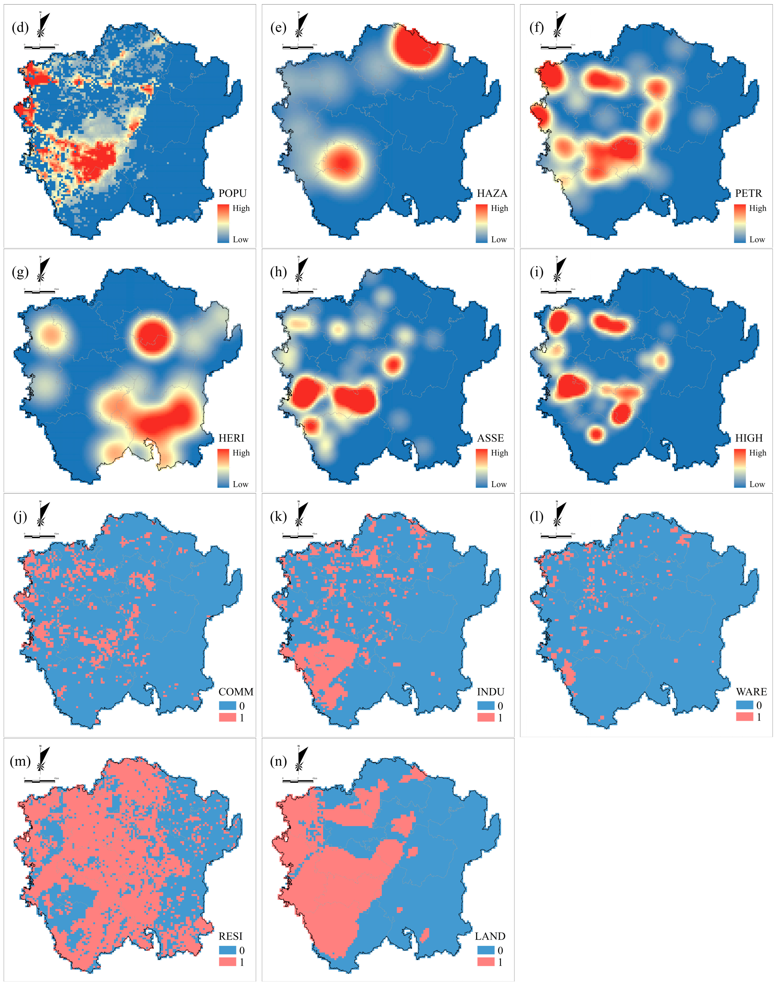
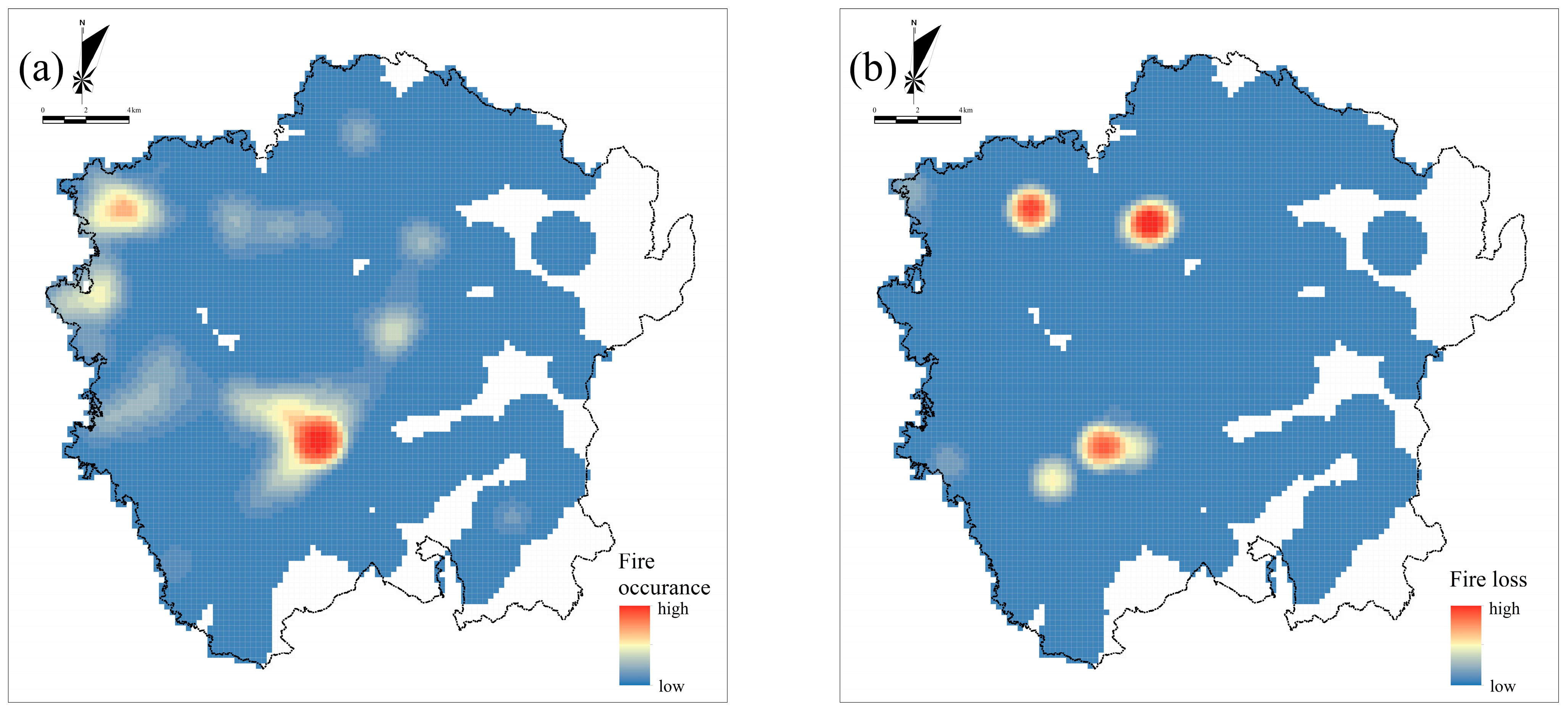
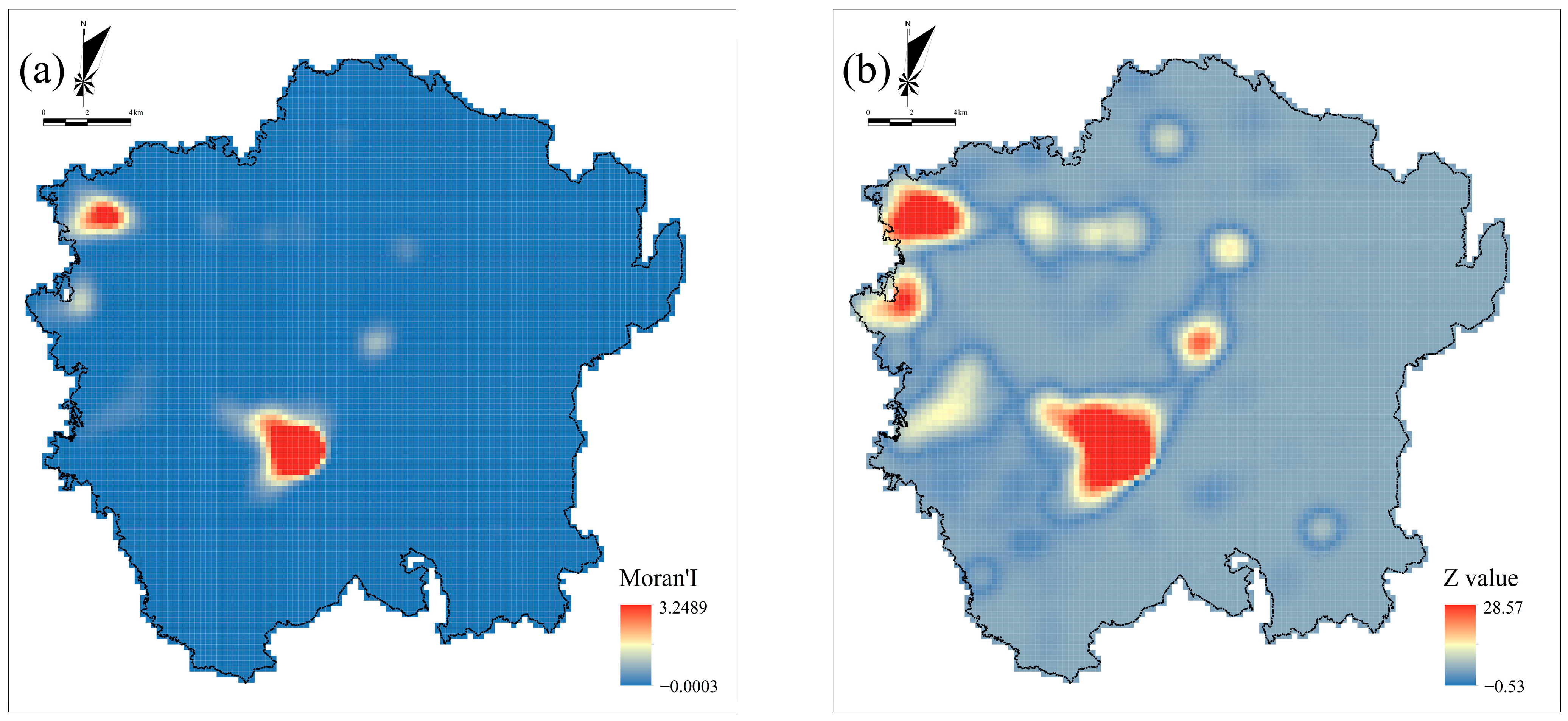
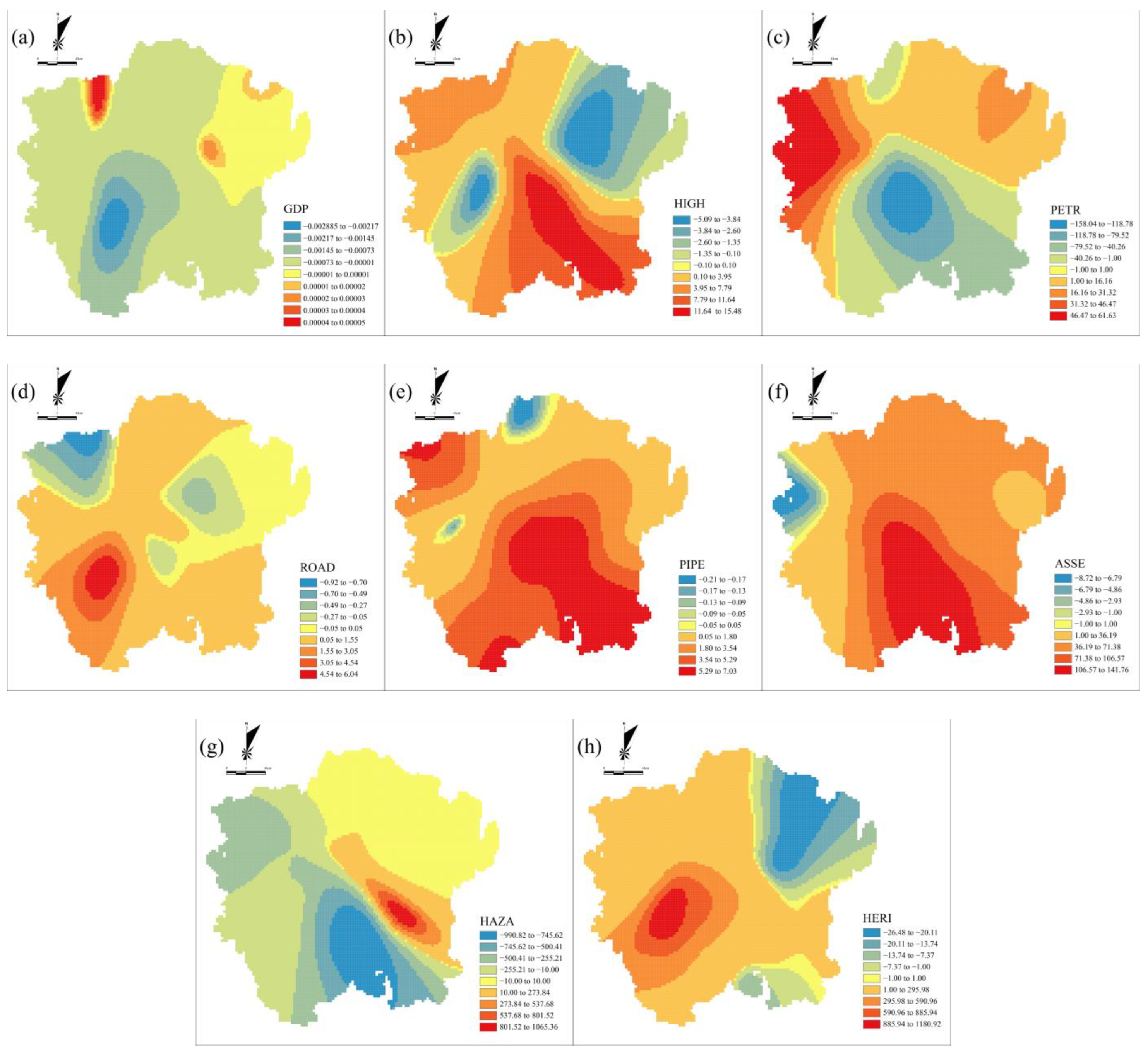
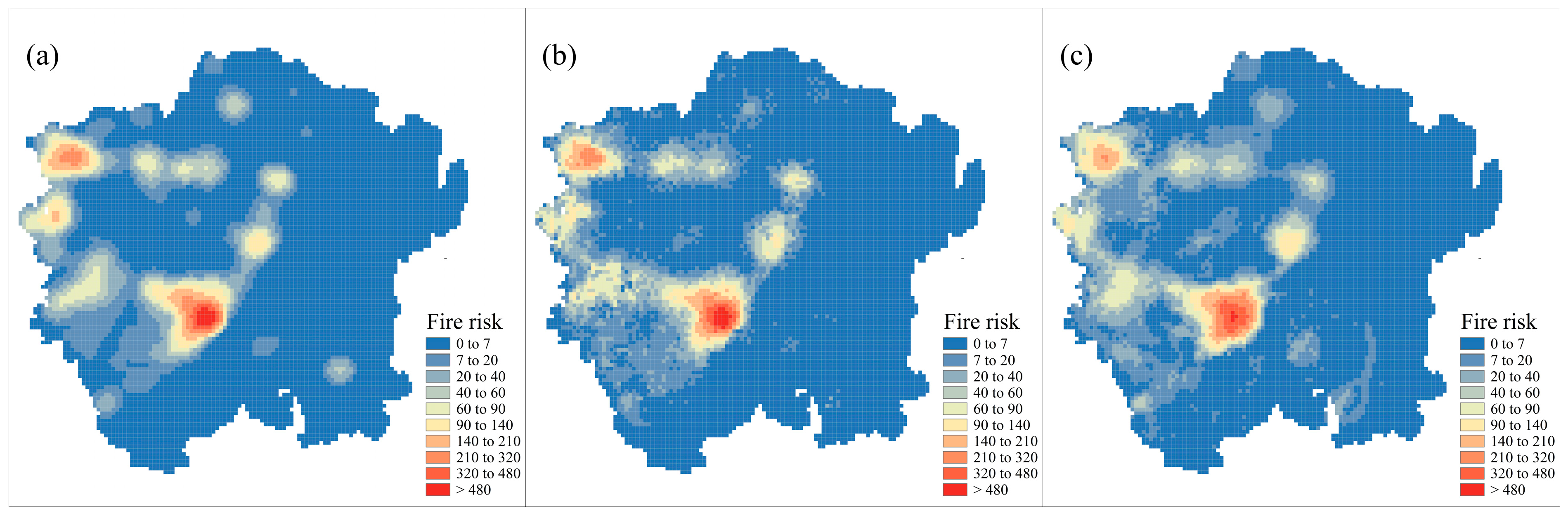
3.3. Spatial Patterns of Indicators and Fire Risk

The spatial association between a variable and its geographical neighbors was measured by Moran’s index of spatial autocorrelation. In spatial correlation analysis, the p-value represents the probability of a random process creating and generating the observed spatial pattern. Z-value means the dispersion of the data set, which helps determine if a particular location exhibits a significant spatial pattern. According to Moran’s I, a Z-score lower than−1.65 means dispersed patterns, a higher than 1.65 means clustered patterns, and else means random patterns, respectively [54,55]. The global Moran’s I of fire risk calculated by using ArcGIS is 0.96, with a Z-value of 183.40 and a P-value of 0. The Moran’s I and Z-value for each grid are extracted and visualized, as shown in Figure 8.

To test the local Moran’s index, the Z-score is utilized as the standard. Based on the extracted data, one immediate observation is that the majority of sample points have positive values for Moran’s I and Z-scores. This indicates that the spatial distribution of fire risk exhibits a “high-high” clustering pattern. In other words, areas with high fire risk tend to cluster together in space. Meanwhile, another observation from the results of the P-value and Z-score indicates that the global Moran index is credible, and the fire risk shows a clustered distribution in the global space.

Unlike the Ordinary Least Squares (OLS) regression model, GWR gives the coefficients for each independent variable at each position. For a better understanding of the spatially varying relationship between the independent variables (fire risk indicators) and dependent variables (fire risk), we created coefficient raster surfaces for each explanatory variable. These surfaces represent the spatial distribution of the coefficients for each independent variable, that is, the strength of the indicators’ influence on the fire risk across different regional locations. The maximum, minimum, and average weight coefficients of each indicator in each grid were calculated based on the distance from the center of the grid image element to all input elements in the neighborhood (bandwidth), as listed in

Table 4. Statistical table of the spatial impact of independent variables.

Variable	Minimum	Maximum	Average
ROAD	−0.91597	6.035046	0.630819
GDP	−0.00289	0.00005	−0.00038
PIPE	−0.20668	7.034545	3.139437
ASSE	−8.72046	141.7564	60.52752
HAZA	−990.822	1065.363	−178.216
PETR	−158.038	61.62599	−14.656
HIGH	−5.08626	15.4803	3.095104
HERI	−26.4821	1180.921	159.7819

. The spatial visualization of the coefficients for the independent variables is presented in Figure 9.

The data from Table 4 indicates that there are significant variations in the impacts of different independent variables on fire risk at the urban spatial grid scale. Among all indicators, the minimum and average weight coefficients of hazardous chemical enterprises are the largest, and the maximum cultural relic protection unit weight coefficient is the largest. Therefore, these two indicators have the greatest impact on the distribution of fire risk among all indicators. Then, following that, variable assembly occupancies, petrol and charging stations, gas pipelines, high-rise buildings, and roads have a relatively smaller impact, while GDP has the smallest impact on the spatial distribution of fire risk. This is different from the contribution ranking of the independent variables to fire risk obtained by the RF model. The possible reason is that the RF model obtains the global coefficient of the independent variable on fire risk, while the GWR model reflects the local change of the independent variable coefficient. Furthermore, as seen in Figure 9, the blue and red regions indicate that the independent variables have a greater impact on the fire risk, while the yellow regions indicate that the independent variables have a smaller impact on the fire risk. The impact of each indicator on fire risk is not uniform globally; however, there are obvious local differences. Therefore, another feature observed is that the spatial distribution of the impact of different independent variables on fire risk is not consistent. In addition, the spatial distribution of the coefficient does not necessarily correspond with the spatial distribution of the independent variable value.

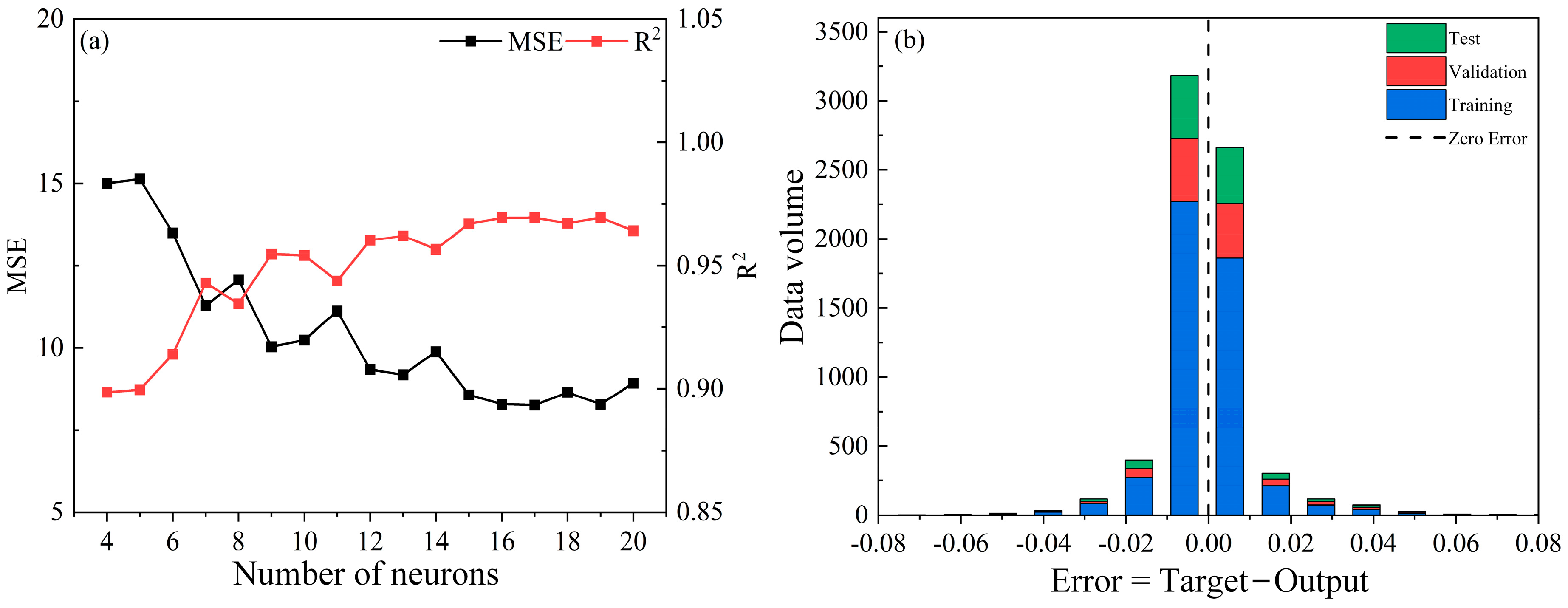
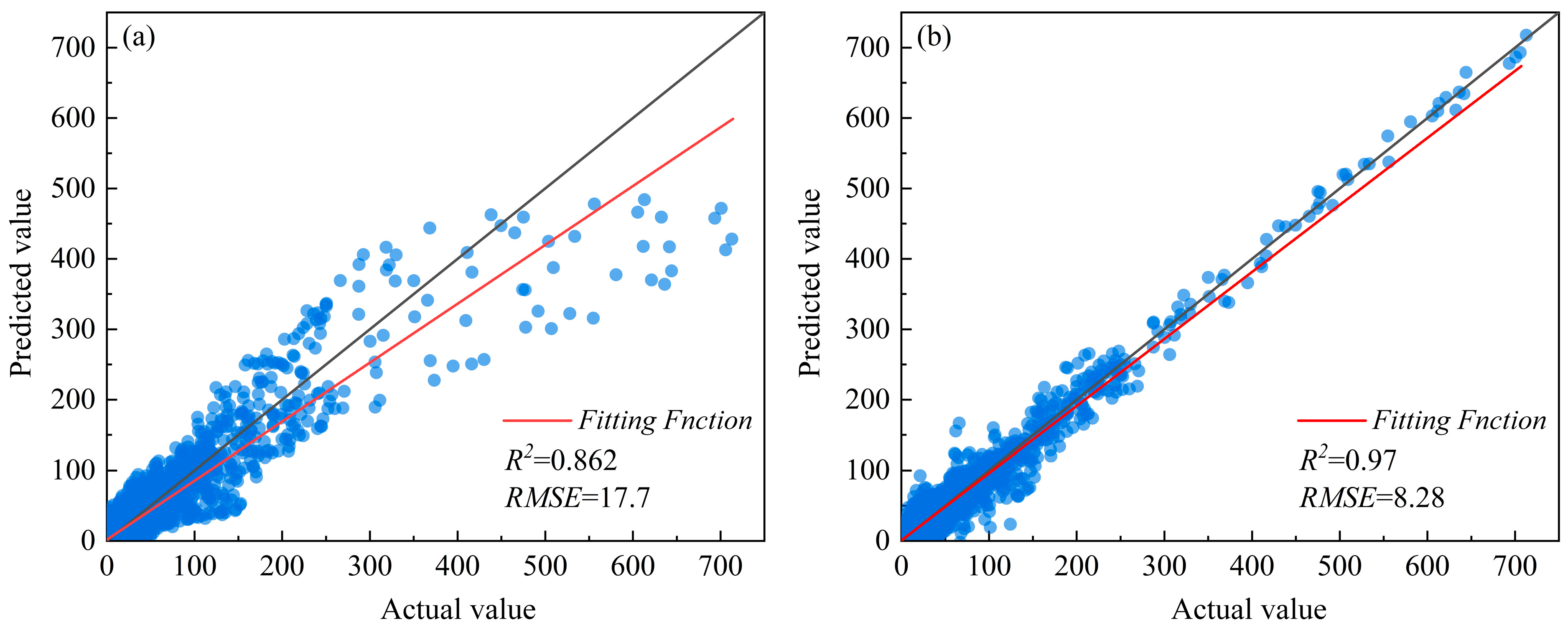
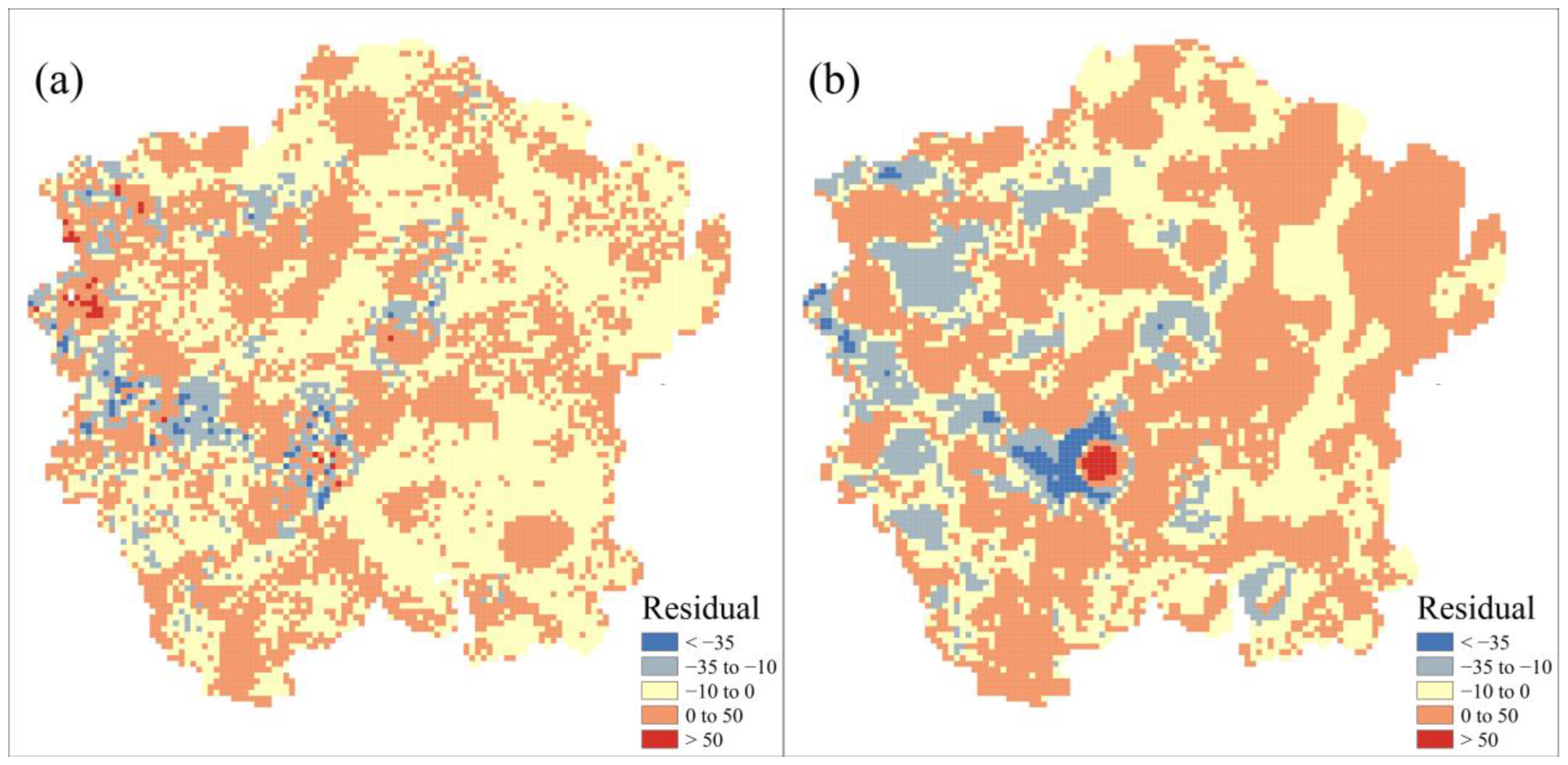
3.4. Comparison of BPNN and GWR Fire Risk Assessment Model

The dataset of the BPNN model is divided into four parts. Three of them are used for training, and the rest for prediction. To ensure the prediction set covers all the raw data, we performed four combinations of tests in total and integrated the BPNN predicted results together. The comparison between actual fire risk and predicted fire risk with the BPNN and GWR models is presented in Figure 10, respectively.

As shown in Figure 10, each scatter point corresponds to the fire risk value of a grid. The x-axis of each scatter point is the actual fire risk value of the grid, and the y-axis is the fire risk value predicted by the model. To facilitate comparison, we superimposed the bisector y = x on the graph. The scattering of points around the bisector indicates the difference between the actual and model-predicted values. In an ideal case, all the points should be distributed along the bisector. Moreover, a linear function is fitted based on the model’s predicted values, which are marked out with a red line. The root-mean-square error (RMSE) is utilized to evaluate the performance of the model.

One conclusion from Figure 10 is that the BPNN model’s performance in predicting fire risk is better than that of the GWR model, which has a value of 0.97 R² and a value of 8.28 RMSE.

To further analyze the reliability of the predicted results of the two models, we extracted and spatially visualized the grid values of the predicted and observed values from BPNN and GWR, respectively. As shown in Figure 11, the left, middle, and right figures show the observed fire risk values, fire risk values obtained from the BPNN predictions, and fire risk values obtained from the GWR predictions. Compared to the GWR model, BPNN provides fire risk assessment results that are more similar to the actual distribution of fire risks.

With these data, it is simply possible to obtain the spatial distribution of the predicted residuals for BPNN and GWR, as presented in Figure 12. To quantify the difference in predicted residuals between these two models, five parts with corresponding interval values are obtained by means of the natural segment point method. The different values of residuals are marked out with blue, light blue, yellow, orange, and red.

With these visualization methods, one of the observations from Figure 12 is that the residual distribution obtained by BPNN is obviously smaller than that obtained by GWR. The grid with larger residual values in the GWR model exhibits spatial clustering, which is predominantly concentrated in areas with higher fire risk. This feature indicates that the reliability and applicability of the GWR model in predicting high-fire-risk regions are inferior to those of the BPNN model.

4. Discussion

This study aims to characterize the spatial distribution of urban fire risk based on regional-scale high-resolution data, considering three factors: urban population, economy, and functional space distribution. A list of key factors is identified through the fire risk feature selection model, which is constructed based on the decision tree algorithm. The spatial pattern variability of fire risk and its impact factors is studied, and the applicability of spatial econometric models and machine learning models in high-resolution urban area fire risk assessment is discussed by comparing GWR models with BPNN models.

One of the contributions is that numerical variables, including ASSE, PETR, GDP, HERI, ROAD, HIGH, HAZA, and PIPE, are the key factors that influenced fire risk in the RF model, with a value of 0.9 R². And during the indicator selection process, it was found that the dummy variables such as WARE, COMM, INDU, and RESI were not effective in explaining fire risk. It may be attributed to the nature of the numerical variables and dummy variables. When estimating micro-scale fire risk, numerical variables provide more precise and detailed information compared to dummy variables. Numerical variables allow for a continuous range of values, which can capture variations and gradients in fire risk more effectively. Dummy variables, on the other hand, are categorical variables that represent different categories or levels of a particular factor. While they are useful for capturing qualitative differences or classifying data into distinct groups, they may not capture the nuanced variations in fire risk that can be expressed by numerical variables. This is similar to previous studies. For example, Song Chao et al. [9]. built a fire risk assessment model with six numerical variables, including distance to fire stations, population, line density of roads, kernel density of enterprise points, yearly average minimum temperature, and elevation. Note that we do not consider influence factors such as elevation and temperature since these indicators differ little at the micro-scale, while numerical variables such as crowded places, GDP, road network density, and high-rise buildings indirectly reflect the region’s population distribution.

The second contribution is that the distribution patterns of the variables and their coefficients of fire risk, at global and local scales, are generally very different. Due to the spatial correlation of data attributes, there are significant variations in the impact of independent variables on fire risk at the grid scale. In general, previous research represented the influence of variables on fire risk in their entire study areas using a unified value [56,57]. However, this type of analysis does not allow detecting and characterizing regional differences in variables’ influences on fire risk distribution; this and the usage of findings have overlooked the importance of localized variations in the influence of variables on fire risk [22]. For example, the distribution of hazardous chemical enterprises and cultural relic protection units has significant variations in their impact on fire risk at different grids, while GDP has the smallest variations on fire risk at different grids. However, on a global scale, GDP shows a greater impact on fire risk based on analysis results. The above analysis is helpful for government managers to determine urban fire risk prevention and control strategies. The independent variable with a large global coefficient but small local variation can be used to determine the fire control strategy of the whole region, while the large global variable with strong local variation can be used to determine the local fire control strategy of the city. For example, GDP is suitable for the fire safety management of the entire region, while hazardous chemical enterprises and cultural relic protection units are suitable for the local region.

The third contribution is that urban fire risk exhibits significant spatial clustering. According to the analysis of the Moran index of fire risk, fire risk shows a “high-high” aggregation phenomenon in most of the grids, i.e., the grids around the grids with high fire risk also had high fire risk, and the GWR model is suitable for modeling and analyzing fire risk.

The fourth contribution of this work reveals that BPNN is more suitable for predicting the micro-scale fire risk distribution in urban areas than GWR. Due to the nonlinear relationships among the various factors contributing to fire occurrences and the spatial correlation in fire risk distribution, it is urgent to develop a fire risk assessment model that can simultaneously capture the nonlinear features and spatial correlation associated with fire risk. The fitting result of the GWR model for fire risk in urban areas is 0.862, which is consistent with previous studies [9,58]. The fitting results of the BPNN model (0.97) are better than GWR. A previous study verified that the performance of the neural network model is better than the logistic regression model in fire risk assessment [59]. The assessment performance of the model indicates that BPNN, as a machine learning model, can not only effectively capture the nonlinearity of fire risks but is also capable of effectively assessing the spatial distribution of fire risks. Therefore, concerning the exploration of the relationship between fire risk and urban fire-related factors at the grid scale in urban areas, although the BPNN model is not adept at extracting spatial relationships from attribute data, its nonlinear entity fitting ability and feature extraction capabilities still exhibit better fitting performance compared to the GWR model.

In summary, the most important finding of this study is the strong correlation between the distribution of urban fire risk and the functional zones, as well as the spatial distribution of critical facilities within a city. Generally speaking, most urban fires are man-made and are affected by human behavior, human activities, and the urban environment. In the past few decades, many researchers have devoted themselves to identifying the factors that contribute to fire risk. However, it is still a challenge to find out all the related factors due to the randomness and uncertainty of fire occurrences and the complexity of human behavior and activities. In addition, sometimes fires occur as a result of the coupling effects of human factors and environmental factors. For example, unsafe behaviors of individuals in an insecure environment, such as smoking in bedrooms without fire alarms and automatic sprinkler systems, can significantly increase the risk of fires. Unsafe behaviors of individuals in a safe environment and safe behaviors of individuals in an unsafe environment may result in relatively lower fire risks across the country. Therefore, it is a new approach that studies fire risk distribution and regional variability through urban functional zoning and feature distribution. With this approach, we do not directly consider the specific factors that cause fires but study the fire risk’s spatial distribution and variability through data related to urban planning. The advantages of this approach lie in two aspects. Firstly, the data required for analysis, such as functional zones and the spatial distribution of critical facilities, are relatively easier to collect. This allows governments to quickly obtain the distribution of fire risk by analyzing such data. Secondly, urban planning is a long-term process, and so is the availability of data. Once the relationship between urban characteristics and the distribution of fire risk is understood, policymakers and decision-makers can incorporate fire risk into urban planning accordingly.

5. Conclusions

The findings of this study contribute to a better understanding of the spatial distribution of urban fire risk, especially the key factors that influence fire risk distribution related to urban functional zoning and feature distribution based on indicator selection and regression modeling methods. The results validated the significant differences in the impact of indicators on the distribution of fire risk in different regions. Since the fire risk indicators are derived from the territorial spatial planning data collected and managed by the government departments, managers can better and more quickly understand the changing trends in fire risk distribution and identify the high-risk areas through changes in the fire risk indicators. Furthermore, territorial spatial planning guides the development of urban space. The results of grid-scale fire risk assessment can be combined with socioeconomic population data on land use development and territorial spatial planning to guide urban fire planning. This integration can further align the development of firefighting infrastructure with urban development, improve the efficiency of urban fire management activities, including prevention, preparedness, adaptation, firefighting, and mitigation of fire consequences, and promote the future development of regional public safety.

Of course, this study also has some limitations. Firstly, the sample size is comparatively small compared to the total number of regions in China; therefore, potential regional differences should be considered. In the following study, we need to collect data from a wider range of areas and explore a greater number of quantitative indicators to achieve more robust results. Secondly, due to limitations in the data obtained, the variables we selected to characterize urban functional layout and infrastructure construction are not comprehensive. In the future, adequate data will allow us to model fire risk spatial distribution through more factors related to urban development and human activity-intensive areas.

References

1. Firefighters Responded to a Record Number of Calls in 2021, Fighting 745,000 Fires. Available online: https://www.119.gov.cn/gk/sjtj/2022/26442.shtml (accessed on 14 July 2022).
2. Rohde, D.; Corcoran, J.; Chhetri, P. Spatial forecasting of residential urban fires: A Bayesian approach. Comput. Environ. Urban Syst. 2010, 34, 58–69. [Google Scholar] [CrossRef]
3. Granda, S.; Ferreira, T.M. Assessing Vulnerability and Fire Risk in Old Urban Areas: Application to the Historical Centre of Guimarães. Fire Technol. 2018, 55, 105–127. [Google Scholar] [CrossRef]
4. Masoumi, Z.; John van, L.G.; Maleki, J. Fire Risk Assessment in Dense Urban Areas Using Information Fusion Techniques. ISPRS Int. J. Geo-Inf. 2019, 8, 579. [Google Scholar] [CrossRef]
5. Silva, D.; Rodrigues, H.; Ferreira, T.M. Assessment and Mitigation of the Fire Vulnerability and Risk in the Historic City Centre of Aveiro, Portugal. Fire 2022, 5, 173. [Google Scholar] [CrossRef]
6. Chhetri, P.; Corcoran, J.; Stimson, R.J.; Inbakaran, R. Modelling Potential Socio-economic Determinants of Building Fires in South East Queensland. Geogr. Res. 2010, 48, 75–85. [Google Scholar] [CrossRef]
7. Wuschke, K.; Clare, J.; Garis, L. Temporal and geographic clustering of residential structure fires: A theoretical platform for targeted fire prevention. Fire Saf. J. 2013, 62, 3–12. [Google Scholar] [CrossRef]
8. Vasiliauskas, D.; Beconytė, G. Spatial Analysis of Fires in Vilnius City in 2010–2012. Geod. Cartogr. 2015, 41, 25–30. [Google Scholar] [CrossRef]
9. Song, C.; Kwan, M.-P.; Song, W.; Zhu, J. A Comparison between Spatial Econometric Models and Random Forest for Modeling Fire Occurrence. Sustainability 2017, 9, 819. [Google Scholar] [CrossRef]
10. Zhang, X.; Yao, J.; Sila-Nowicka, K.; Jin, Y. Urban Fire Dynamics and Its Association with Urban Growth: Evidence from Nanjing, China. ISPRS Int. J. Geo-Inf. 2020, 9, 218. [Google Scholar] [CrossRef]
11. Chen, Y.; Wu, G.; Chen, Y.; Xia, Z. Spatial Location Optimization of Fire Stations with Traffic Status and Urban Functional Areas. Appl. Spat. Anal. Policy 2023, 16, 771–788. [Google Scholar] [CrossRef]
12. Jin, G.; Wang, Q.; Zhu, C.; Feng, Y.; Huang, J.; Hu, X. Urban Fire Situation Forecasting: Deep sequence learning with spatio-temporal dynamics. Appl. Soft Comput. 2020, 97, 106730. [Google Scholar] [CrossRef]
13. Rahman Tishi, T.; Islam, I. Urban fire occurrences in the Dhaka Metropolitan Area. GeoJournal 2018, 84, 1417–1427. [Google Scholar] [CrossRef]
14. Wang, K.; Yuan, Y.; Chen, M.; Wang, D. A POIs based method for determining spatial distribution of urban fire risk. Process Saf. Environ. Prot. 2021, 154, 447–457. [Google Scholar] [CrossRef]
15. Orusa, T.; Viani, A.; Moyo, B.; Cammareri, D.; Borgogno-Mondino, E. Risk Assessment of Rising Temperatures Using Landsat 4–9 LST Time Series and Meta® Population Dataset: An Application in Aosta Valley, NW Italy. Remote Sens. 2023, 15, 2348. [Google Scholar] [CrossRef]
16. Kumar, V.; Jana, A.; Ramamritham, K. A decision framework to assess urban fire vulnerability in cities of developing nations: Empirical evidence from Mumbai. Geocarto Int. 2020, 37, 543–559. [Google Scholar] [CrossRef]
17. Bernardini, G.; Quagliarini, E.; D’Orazio, M. Towards creating a combined database for earthquake pedestrians’ evacuation models. Saf. Sci. 2016, 82, 77–94. [Google Scholar] [CrossRef]
18. Tomar, S.K.; Kaur, A.; Dangi, H.K. Impact of Spatial–Temporal Variations on Fire Vulnerability: A Case Study of the South-West Division of Delhi, India. In Risk Analysis XI; WIT Press: Southampton, UK, 2018; pp. 273–282. [Google Scholar]
19. Turner, S.L.; Johnson, R.D.; Weightman, A.L.; Rodgers, S.E.; Arthur, G.; Bailey, R.; Lyons, R.A. Risk factors associated with unintentional house fire incidents, injuries and deaths in high-income countries: A systematic review. Inj. Prev. 2017, 23, 131–137. [Google Scholar] [CrossRef] [PubMed]
20. Tomar, S.; Kaur, A.; Sarma, K.; Dangi, H. Fire risk assessment and fire hazard zonation mapping using GIS in South-West division of Delhi. J. Adv. Res. Appl. 2018, 5, 213–220. [Google Scholar]
21. Hastie, C.; Searle, R. Socio-economic and demographic predictors of accidental dwelling fire rates. Fire Saf. J. 2016, 84, 50–56. [Google Scholar] [CrossRef]
22. Parente, J.; Pereira, M.G.; Amraoui, M.; Tedim, F. Negligent and intentional fires in Portugal: Spatial distribution characterization. Sci. Total Environ. 2018, 624, 424–437. [Google Scholar] [CrossRef] [PubMed]
23. Aven, T.; Guikema, S. Whose uncertainty assessments (probability distributions) does a risk assessment report: The analysts’ or the experts’? Reliab. Eng. Syst. Saf. 2011, 96, 1257–1262. [Google Scholar] [CrossRef]
24. Gehandler, J.; Ingason, H.; Lönnermark, A.; Frantzich, H.; Strömgren, M. Performance-based design of road tunnel fire safety: Proposal of new Swedish framework. Case Stud. Fire Saf. 2014, 1, 18–28. [Google Scholar] [CrossRef]
25. Dong, Y.; Frangopol, D.M. Probabilistic ship collision risk and sustainability assessment considering risk attitudes. Struct. Saf. 2015, 53, 75–84. [Google Scholar] [CrossRef]
26. Chen, J.; Wang, X.; Yu, Y.; Yuan, X.; Quan, X.; Huang, H. Improved Prediction of Forest Fire Risk in Central and Northern China by a Time-Decaying Precipitation Model. Forests 2022, 13, 480. [Google Scholar] [CrossRef]
27. McCarty, J.; Francis, R.; Fain, J.; Haynes, K. Wildfire Risk Models for Western Greenland: Geostatistical Considerations. In EGU General Assembly Conference Abstracts, Proceedings of the 22nd EGU General Assembly, Online, 4–8 May 2020; EDU: Munich, Germany, 2020; p. 12660. [Google Scholar]
28. Hegde, J.; Rokseth, B. Applications of machine learning methods for engineering risk assessment—A review. Saf. Sci. 2020, 122, 104492. [Google Scholar] [CrossRef]
29. Guha, S.; Jana, R.K.; Sanyal, M.K. Artificial neural network approaches for disaster management: A literature review. Int. J. Disaster Risk Reduct. 2022, 81, 103276. [Google Scholar] [CrossRef]
30. Xiong, J.; Sun, M.; Zhang, H.; Cheng, W.; Yang, Y.; Sun, M.; Cao, Y.; Wang, J. Application of the Levenburg–Marquardt back propagation neural network approach for landslide risk assessments. Nat. Hazards Earth Syst. Sci. 2019, 19, 629–653. [Google Scholar] [CrossRef]
31. Li, S.; Bi, F.; Chen, W.; Miao, X.; Liu, J.; Tang, C. An Improved Information Security Risk Assessments Method for Cyber-Physical-Social Computing and Networking. IEEE Access 2018, 6, 10311–10319. [Google Scholar] [CrossRef]
32. Wu, Y.; Li, X.; Liu, Q.; Tong, G. The Analysis of Credit Risks in Agricultural Supply Chain Finance Assessment Model Based on Genetic Algorithm and Backpropagation Neural Network. Comput. Econ. 2021, 60, 1269–1292. [Google Scholar] [CrossRef]
33. Feng, Y.; Souri, A. Bank Green Credit Risk Assessment and Management by Mobile Computing and Machine Learning Neural Network under the Efficient Wireless Communication. Wirel. Commun. Mob. Comput. 2022, 2022, 3444317. [Google Scholar] [CrossRef]
34. Ting, L.; Man, Z.; Yuhan, J.; Sha, S.; Yiqiong, J.; Minzan, L. Management of CO2 in a tomato greenhouse using WSN and BPNN techniques. Int. J. Agric. Biol. Eng. 2015, 8, 43–51. [Google Scholar]
35. Bistinas, I.; Oom, D.; Sa, A.C.; Harrison, S.P.; Prentice, I.C.; Pereira, J.M. Relationships between human population density and burned area at continental and global scales. PLoS ONE 2013, 8, e81188. [Google Scholar] [CrossRef] [PubMed]
36. Jennings, C.R. Social and economic characteristics as determinants of residential fire risk in urban neighborhoods: A review of the literature. Fire Saf. J. 2013, 62, 13–19. [Google Scholar] [CrossRef]
37. Sarvia, F.; De Petris, S.; Borgogno-Mondino, E. Exploring Climate Change Effects on Vegetation Phenology by MOD13Q1 Data: The Piemonte Region Case Study in the Period 2001–2019. Agronomy 2021, 11, 555. [Google Scholar] [CrossRef]
38. Orusa, T.; Cammareri, D.; Borgogno Mondino, E.B. A Possible Land Cover EAGLE Approach to Overcome Remote Sensing Limitations in the Alps Based on Sentinel-1 and Sentinel-2: The Case of Aosta Valley (NW Italy). Remote Sens. 2022, 15, 178. [Google Scholar] [CrossRef]
39. Rausand, M. Risk Assessment: Theory, Methods, and Applications; John Wiley & Sons: Hoboken, NJ, USA, 2013; Volume 115. [Google Scholar]
40. Yoe, C. Principles of Risk Analysis: Decision Making under Uncertainty; CRC Press: Boca Raton, FL, USA, 2019. [Google Scholar]
41. Matellini, D.B.; Wall, A.D.; Jenkinson, I.D.; Wang, J.; Pritchard, R. Modelling dwelling fire development and occupancy escape using Bayesian network. Reliab. Eng. Syst. Saf. 2013, 114, 75–91. [Google Scholar] [CrossRef]
42. Silverman, B.W. Density Estimation for Statistics and Data Analysis; Routledge: Abingdon, UK, 2018. [Google Scholar]
43. Oliveira, S.; Oehler, F.; San-Miguel-Ayanz, J.; Camia, A.; Pereira, J.M.C. Modeling spatial patterns of fire occurrence in Mediterranean Europe using Multiple Regression and Random Forest. For. Ecol. Manag. 2012, 275, 117–129. [Google Scholar] [CrossRef]
44. Lee, S.; Kim, J.-C.; Jung, H.-S.; Lee, M.J.; Lee, S. Spatial prediction of flood susceptibility using random-forest and boosted-tree models in Seoul metropolitan city, Korea. Geomat. Nat. Hazards Risk 2017, 8, 1185–1203. [Google Scholar] [CrossRef]
45. Čeh, M.; Kilibarda, M.; Lisec, A.; Bajat, B. Estimating the Performance of Random Forest versus Multiple Regression for Predicting Prices of the Apartments. ISPRS Int. J. Geo-Inf. 2018, 7, 168. [Google Scholar] [CrossRef]
46. Zhang, Y.; Zhang, R.; Ma, Q.; Wang, Y.; Wang, Q.; Huang, Z.; Huang, L. A feature selection and multi-model fusion-based approach of predicting air quality. ISA Trans. 2020, 100, 210–220. [Google Scholar] [CrossRef]
47. Haykin, S. Neural Networks and Learning Machines; Pearson: Upper Saddle River, NJ, USA, 2009; Volume 3. [Google Scholar]
48. Foster, S.A.; Gorr, W.L.J.M.S. An adaptive filter for estimating spatially-varying parameters: Application to modeling police hours spent in response to calls for service. Manag. Sci. 1986, 32, 878–889. [Google Scholar] [CrossRef]
49. Brunsdon, C.; Fotheringham, A.S.; Charlton, M.E. Geographically weighted regression: A method for exploring spatial nonstationarity. Geogr. Anal. 1996, 28, 281–298. [Google Scholar] [CrossRef]
50. Fotheringham, A.S.; Charlton, M.E.; Brunsdon, C.J.E. Geographically weighted regression: A natural evolution of the expansion method for spatial data analysis. Environ. Plan. A 1998, 30, 1905–1927. [Google Scholar] [CrossRef]
51. Buyantuyev, A.; Wu, J. Urban heat islands and landscape heterogeneity: Linking spatiotemporal variations in surface temperatures to land-cover and socioeconomic patterns. Landsc. Ecol. 2009, 25, 17–33. [Google Scholar] [CrossRef]
52. Anselin, L. The Moran Scatterplot as an ESDA Tool to Assess Local Instability in Spatial Association; Regional Research Institute, West Virginia University: Morgantown, WV, USA, 1993. [Google Scholar]
53. Kanaroglou, P.S.; Adams, M.D.; De Luca, P.F.; Corr, D.; Sohel, N. Estimation of sulfur dioxide air pollution concentrations with a spatial autoregressive model. Atmos. Environ. 2013, 79, 421–427. [Google Scholar] [CrossRef]
54. Baller, R.D.; Anselin, L.; Messner, S.F.; Deane, G.; Hawkins, D.F.J.C. Structural covariates of US county homicide rates: Incorporating spatial effects. Criminology 2001, 39, 561–588. [Google Scholar] [CrossRef]
55. Dong, L.; Liang, H. Spatial analysis on China’s regional air pollutants and CO2 emissions: Emission pattern and regional disparity. Atmos. Environ. 2014, 92, 280–291. [Google Scholar] [CrossRef]
56. Xie, L.; Zhang, R.; Zhan, J.; Li, S.; Shama, A.; Zhan, R.; Wang, T.; Lv, J.; Bao, X.; Wu, R. Wildfire Risk Assessment in Liangshan Prefecture, China Based on An Integration Machine Learning Algorithm. Remote Sens. 2022, 14, 4592. [Google Scholar] [CrossRef]
57. Guo, J.; Lu, L.; Dong, Y.; Huang, W.; Zhang, B.; Du, B.; Ding, C.; Ye, H.; Wang, K.; Huang, Y.; et al. Spatiotemporal Distribution and Main Influencing Factors of Grasshopper Potential Habitats in Two Steppe Types of Inner Mongolia, China. Remote Sens. 2023, 15, 866. [Google Scholar] [CrossRef]
58. Shah-Heydari Pour, A.; Pahlavani, P.; Bigdeli, B. Providing the Fire Risk Map in Forest Area Using a Geographically Weighted Regression Model with Gaussin Kernel and Modis Images, a Case Study: Golestan Province. Int. Arch. Photogramm. Remote Sens. Spat. Inf. Sci. 2017, XLII-4/W4, 477–481. [Google Scholar] [CrossRef]
59. Jafari Goldarag, Y.; Mohammadzadeh, A.; Ardakani, A.S. Fire Risk Assessment Using Neural Network and Logistic Regression. J. Indian Soc. Remote Sens. 2016, 44, 885–894. [Google Scholar] [CrossRef]
Figure 1. (a) Overview of the location of this study area in Chengdu; (b) Schematic diagram for urban development boundary; (c) Distribution of land-use types; (d) Grading diagram of this study area.
Ijgi 12 00404 g001
Figure 2. Distribution of independent variables in Longquanyi District (a) Road, (b) Gas pipelines, (c) GDP, (d) Population, (e) Hazardous chemical enterprises, (f) Petrol and charging stations, (g) Cultural heritage protection unit, (h) Assembly occupancies, (i) High-rise building; (j) Commercial service zone; (k) Industrial zone; (l) Warehouse zone; (m) Res-idential zone; (n) Land development intensity.
Ijgi 12 00404 g002aIjgi 12 00404 g002b
Figure 3. The distributions of fire occurrence and fire loss in the Longquanyi District are: (a) kernel density of fire occurrence; (b) kernel density of fire loss; (c) actual fire occurrence; and (d) actual fire loss.
Ijgi 12 00404 g003aIjgi 12 00404 g003b
Figure 4. BPNN structure [47].
Ijgi 12 00404 g004
Figure 5. Number of hidden layer neurons and simulation results: (a) Number of hidden layer neurons; (b) Final error of the model.
Ijgi 12 00404 g005
Figure 6. The optimal subset of independent variables with the number of variables (a) RF, (b) GBDT, and (c) XGBoost.
Ijgi 12 00404 g006
Figure 7. Importance of each indicator: (a) RF, (b) GBDT, (c) XGBoost.
Ijgi 12 00404 g007
Figure 8. The visualization of (a) local Moran’s I and (b) significance test results.
Ijgi 12 00404 g008
Figure 9. Coefficient rasterization of independent variables (a) GDP; (b) High-rise buildings; (c) Petrol and charging stations; (d) Road, (e) Gas pipeline, (f) Assembly occupancies; (g) Hazardous chemical enterprises; and (h) Cultural heritage protection units.
Ijgi 12 00404 g009
Figure 10. Correlation analysis between actual and predicted values of (a) the GWR model and (b) the BPNN model.
Ijgi 12 00404 g010
Figure 11. Comparison of prediction effects of models: (a) actual value; (b) BPNN predicted value; (c) GWR predicted value.
Ijgi 12 00404 g011
Figure 12. Spatial distribution and visualization results of model residuals (a) BPNN (b) GWR.
Ijgi 12 00404 g012