Measuring COVID-19 Vulnerability for Northeast Brazilian Municipalities: Social, Economic, and Demographic Factors Based on Multiple Criteria and Spatial Analysis

Abstract

COVID-19 has brought several harmful consequences to the world from many perspectives, including social, economic, and well-being in addition to health issues. However, these harmful consequences vary in intensity in different regions. Identifying which cities are most vulnerable to COVID-19 and understanding which variables could be associated with the advance of registered cases is a challenge. Therefore, this study explores and builds a spatial decision model to identify the characteristics of the cities that are most vulnerable to COVID-19, taking into account social, economic, demographic, and territorial aspects. Hence, 18 features were separated into the four groups mentioned. We employed a model joining the dominance-based rough set approach to aggregate the features (multiple criteria) and spatial analysis (Moran index, and Getis and Ord) to obtain final results. The results show that the most vulnerable places have characteristics with high population density and poor economic conditions. In addition, we conducted subsequent analysis to validate the results. The case was developed in the northeast region of Brazil.

1. Introduction

SARS-CoV-2, the coronavirus that caused the COVID-19 pandemic, was discovered in December 2019. The first known cases were detected in samples obtained from a patient from Wuhan, Hubei province (China), who had pneumonia of a then-unknown origin. The phylogenetic homogeneity of SARS-CoV-2 has characteristics that are distinct from those of other human respiratory viruses such as SARS-CoV, MERS-CoV, and the seasonal influenza virus [1,2]

The virus quickly spread worldwide, and in 2020, the World Health Organization (WHO) declared an outbreak. The outbreak of the new coronavirus reached Latin American countries later than other continents. In Brazil, the first case was confirmed on 26 February [3], and community transmission was detected on 13 March [4]. Nonetheless, in 2021, Brazil has been among the countries with the most cases and deaths registered, remaining third in the rankings in 2022 [5]. The high ranking is attributable to inefficient crisis management standards within the Brazilian national government [6,7] and local governments (states and municipalities), use of unsuitable tools for epidemiological surveillance [8], insufficient measures to implement social distancing [4], and scarce RT-PCR testing and diagnoses [9]. Also, limited resources bring large pressure on health system facilities [10]. The first wave of the pandemic in Brazil started in its principal cities (the largest and most affluent cities with intense economic activities), especially in São Paulo and Rio de Janeiro [4]. Eventually, the virus spread to smaller cities, and unfortunately, unlike urban centers, these cities have a scarcity of medical supplies, health facilities, hospitals, beds, and health professionals [11].

The diversity of societal issues caused by COVID-19 requires research from different perspectives. One of these concerns is the association between COVID-19 propagation and economic, demographic, and environmental factors, e.g., comparing the incidence of the disease in urban and rural municipalities according to local features [12], taking into account the aspect of the vaccination policies of the demographic [13] and verifying the size of towns corroborated to the spread of the virus [7]. Another issue that deserves further discussion is the geographic spatial aspects. The research conducted in [14] shows that the spread of COVID-19 has occurred more in urban areas with high inhabitant density than in rural areas. However, the density cannot be considered as the unique explanation for a high number of COVID-19 cases, as demonstrated in [15]. In Brazil, the factors driving the spread of COVID-19 were supposedly mostly unknown in the early stages and checked afterwards to be related to the movement of people ahead of several other factors [16].

Considering the context and knowledge about similar situations involving contagious diseases, this paper explores and identifies socially vulnerable groups, for whom socioeconomic and environmental questions in relation to COVID-19 would be highly relevant. Therefore, a spatial decision model (multiple criteria evaluation and clusters spatial analysis) was structured to determine vulnerable municipalities in the northeast region of Brazil, based on social, economic, territorial, and demographic aspects. With this framework, plans to provide solutions to regions that are most vulnerable to COVID-19 must then be devised and enacted.

2. Theoretical Review

Since the outbreak was declared a pandemic, researchers from diverse fields have conducted academic projects to contribute to and propose solutions to avoid the harmful effects of COVID-19. In this section, we explore the relationship between COVID-19 and social, economic, territorial, and demographic features to support the objective of this study.

In one of the first such studies, [17] conducted a geospatial analysis of COVID-19 in Germany involving 368 variables to identify patterns among geographic, socioeconomic, infrastructure, and environmental characteristics. They determined a strong association between COVID-19 and churches, unemployment registries, and public transport stations. In a study on Beijing, [18] identified demographic density and distances within manufacturing areas, hospitals, financial centers, industrial neighborhoods, educational facilities (museums, schools, and libraries), and shopping centers as relevant features. A vulnerability index was proposed by [19], considering variables such as population density, unemployment, and health status (obesity or diabetes).

In [20], smartphone mobility technology was used in Delhi, India to track patients with symptoms. However, the unavailability of smartphones and barriers related to social, economic, territorial, and demographic aspects contributed to creating an exclusionary environment in some areas. In a study on the United States, registered COVID-19 cases were correlated with socioeconomic data using cluster analysis and geospatial regression [21]. They revealed that age, race, occupation, and living in vulnerable situations are important for identifying the susceptibility of a population to COVID-19. In addition, correctly selected variables may be useful to provide valuable information for developing targeted interventions for certain areas and periods as demonstrated in [22].

Similar studies have also been conducted regarding Brazil, demonstrating the association between COVID-19 cases and several variables. In [4], all Brazilian territories were mapped, locating which urban centers were disadvantaged and which regions were nearby. Places with higher densities also accelerated the spread of the disease. Similar results were obtained for Salvador, the most populous principal city of the Brazilian northeast, which included economic disparities and race as relevant factors [23].

Brazilian research papers on each northeast state have been published. In the state of Ceará, spatial clusters and the human development index had a positive association with COVID-19 cases [24]. In Fortaleza (the capital of the state of Ceará), there was evidence that spread of the disease started in a neighborhood with a wide socioeconomic profile, including poor groups and high population density [25]. Similar results were obtained for the Recife municipality, in the state of Pernambuco [26]. In Salvador (the capital of the state of Bahia), areas with better economic conditions were at an advantage in relation to the contagiousness of the disease [27].

Understanding these associations contributes as a reference for the creation of public health policies in related collective welfare. From this perspective, a methodology should be constructed with these associations as an underlying principle for consistent results.

Table 1. Summary of Brazilian research papers correlating social, economic, and demographic aspects with COVID-19.

Objective	Approaches	Factors	Spatial Units	Findings	References
COVID index to verify capability of hospital structures to deal with COVID-19	Data envelopment analysis (DEA) approach	Respirators Intensive care units (ICU) Hospital beds Physicians Nurses	Microregional administrative units	Patterns of socioeconomics inequalities	[11]
Comparison of SARS before and during COVID-19	Logistic regression model	Municipal human development index Proportion of population vulnerable to poverty Proportion of extremely poor Presence of federal highways	Macroregional health offices Municipalities	High population density and urban mobility are the factors that most contribute to the spread of COVID-19	[28]
Identify data gaps in large slum communities, considering socio-economic, demographic, and physical variables	Earth observation (EO) (satellites images)	Population Buildings Road and pathway types Local markets Health facilities	Pixels	Provides guidelines on which locals need further investigation via EO and gathers procedures to support COVID-19 responses	[29]
Trends in analyses of social distancing and living conditions based on the social distancing index and living conditions index of municipalities	Aggregated score	Distribution of residents by per-capita monthly income Proportion of black people Schooling rate Households connected to regular water supply network	Neighborhood	Social distancing measures must consider the place; the most vulnerable neighborhoods are weak at responding to the pandemic	[27]
Identify most vulnerable areas, considering risk of arrival cases and local transmission	Probabilistic models and multivariate cluster analysis	Population per age group Infant mortality Life expectancy GINI index	Microregional administrative units	Several microregional administrative units considered as vulnerable	[4]
Employ additive models into spatial patterns considering factors such as race/ethnicity, service occupation, and household size	Generalized additive models and Poisson framework	Race/ethnicity, service occupation household size, cases, and hospitalizations	Cities	Percent minority, average household size, and percent service industry keep positive association with COVID-19 risk	[30]
Explore spatial patterns (initial stages) of COVID-19 cases with social determinants	Density spatial analysis and statistical correlation	COVID-19 incidence, asthma cases, per capt income, education, housing, multiple unit structures	Counties	Greatest number of cases associated with senior living facilities, cases in places with high population density and asthma hospitalization	[31]

presents a summary of Brazilian research papers, with a focus on consolidating social, economic, and demographic data.

3. Data and Methods

The methodology presented in this paper follows a linear step-by-step procedure, comprising data gathering, selection of locality to study, pre-analysis, spatial modelling, and analysis of outcomes. Our study objectively investigates a set of variables which characterize the municipalities, taking into account the COVID-19 case records and performs a classification procedure to measure the vulnerability level. A holistic approach was used to build a multicriteria model, and decision rules were generated to classify the municipalities and adapted from [32]. Throughout this process, spatial analysis was conducted in two phases to ensure better results. The proposed method follows four steps: (a) data treatment, (b) variable exploration, (c) multiple-criteria decision model, and (d) spatial inference.

3.1. Data Treatment

In the first step, the municipalities to be analyzed were defined, and their representative features were selected. Before achieving these features, we investigated similar studies using multiple criteria evaluation in a COVID context. In [33], the analytical hierarchy process (AHP) method was employed to establish a regional vulnerability index for the COVID-19 virus, considering criteria such as: population density, permanent resident population, passengers-kilometers, and the numbers of students with a college degree or above. In [34], 15 features were used to model COVID-19 vulnerability using a GIS platform and AHP method. In addition to the social criteria used (population density and urban population), physical vulnerability (hospital and road network) and epidemiological (active cases, vaccinated people, and total deaths) criteria were included. The AHP was employed to prioritize policies against COVID-19 in Turkey, which included aspects such as gender, age, and occupation [35]. In [36], the GIS and multiple criteria evaluation were used for the vulnerability index analysis also with criteria such as social and urban characteristics. All these finds have shown a satisfactory analysis with the features used.

We built a set of explanatory variables, which are associated with the spread of COVID-19, based on five aspects: social, economic, demographic, territorial, and COVID-19 cases. From these aspects, a set of 19 variables were defined (

Table 2. Attributes used in the study.

Variable	Description
Pop_estim	Absolute population in estimated values per municipality
Peop_ocup	Percentage of total population that are currently employed ([number of employed individuals in the municipality/total population of the municipality × 100) (2019)
Income_m	Average monthly income of formal workers (2019) BRL USD
Pop_ocu	Number of employed people in the municipality (%) (2019)
Income_prop	Percentage of population with nominal monthly income per capita of up to 1/2 minimum wage: [Population residing in permanent private households with monthly income of up to 1/2 minimum wage/Total population residing in permanent private households] × 100 (2010)
Esco_1	Absolute number of schools that offer basic education in the municipality (2020)
Escol_2	Absolute number of schools offering secondary education in the municipality (2020)
MHDI	Municipal human development index, based on the following dimensions: income, education, and health (2010)
GPD	Gross domestic product (2018)
Schollar_prop	[Population residing in the municipality aged 6 to 14 years old enrolled in regular education/Total population residing in the municipality aged 6 to 14 years old] × 100 (2010)
SUS	Establishments that offer basic health services and are part of the Unified Health System [Sistema Único de Saúde] (2009).
Sewage	[Total resident population in permanent private households with sewage system belonging to the general network and septic tank/Total resident population in permanent private households] × 100 (2010)
Area	Total area of the municipality based on rural areas, urban areas, urban core, rural core, and urban areas with high densities of buildings
Area1	Total area of the municipality based on urban core, rural core, urban areas with high densities of buildings, and urban areas with low densities of buildings
Area2	Total area of the municipality based on urban core and urban areas with high densities of buildings
Den	Population density: [Absolute population in estimated values by municipality/Area]
Den 1	Population density1: [Absolute population in estimated values by municipality/Area2]
Den 2	Population density2: [Absolute population in estimated values by municipality/Area3]
COVID-19 registers	Daily COVID-19 cases included as attribute feature

). The features include aspects regarding population, demographic density, employment rate, educational level, household income, the human development index (HDI), the gross domestic product (GDP) and poverty. Primary data were collected from the Brazilian Institute of Geography and Statistics [37]. Lastly, the territorial perspective concerns the subdivisions of each municipality (urbanization and rural zones). Each Brazilian city has several administrative divisions (census tracts, neighborhoods, counties borders, etc.). For the present study, areas of space were obtained using a combination of rural x urban x high density features, characterizing three categories of counties. The first considers territories of all counties as space variable. The second considers only territories with urbanization (high and low settlement), while the third variable considers only areas with high densities of buildings (having calculated the density of inhabitants). In total, we explored a set of 19 features which are described in Table 2. Additionally, data regarding COVID-19 registers (daily case reports) were also explored as a possible feature.

3.2. Variable Exploration

In step (b), we explored the correlation between the selected features and COVID-19 records by means of statistical and spatial analysis. Firstly, we investigated the relationship using the ordinary least square (OLS) regression approach and with Spearman’s rank correlation coefficient. Furthermore, we used spatial autocorrelation analysis to evaluate the spatial clustering patterns of COVID-19 registries via Global Moran’s I index [38] for several weeks, so that the behavior of the spread of the disease could be examined along with the evolution of new records. Regarding inference, spatial analysis was also used considering vaccination hesitancy correlated with factors such as per capita income, age, mobile homes, and uninsured people. This index was employed as follows (Equation (1)):

$$I=\frac{n{{\displaystyle \sum }}_{i=1}^n{{\displaystyle \sum }}_{j=1}^n{W}_{ij}\left(X_i-\overline{X}\right)\left(X_j-\overline{X}\right)}{{{\displaystyle \sum }}_{i=1}^{n }{{\displaystyle \sum }}_{j=1}^n{W}_{ij}{{\displaystyle \sum }}_{i=1}^n{\left(X_i-\overline{X}\right)}^2},$$

(1)

where $W_{ij}$ represents the weights of the spatial relationship between elements $I$ and $j$, ($X_i-\overline{X}$) represents the deviation of the attribute value of element $i$ from its mean, and $n$ denotes the total number of elements. The value of Global Moran’s I is within the range [−1, 1]. If the index has a value close to 0, then the distribution of COVID-19 cases has a random pattern. If the index is close to −1, the virus spread has a dispersed distribution, whereas if the index is close to 1, the pattern of COVID-19 cases is clustered [18].

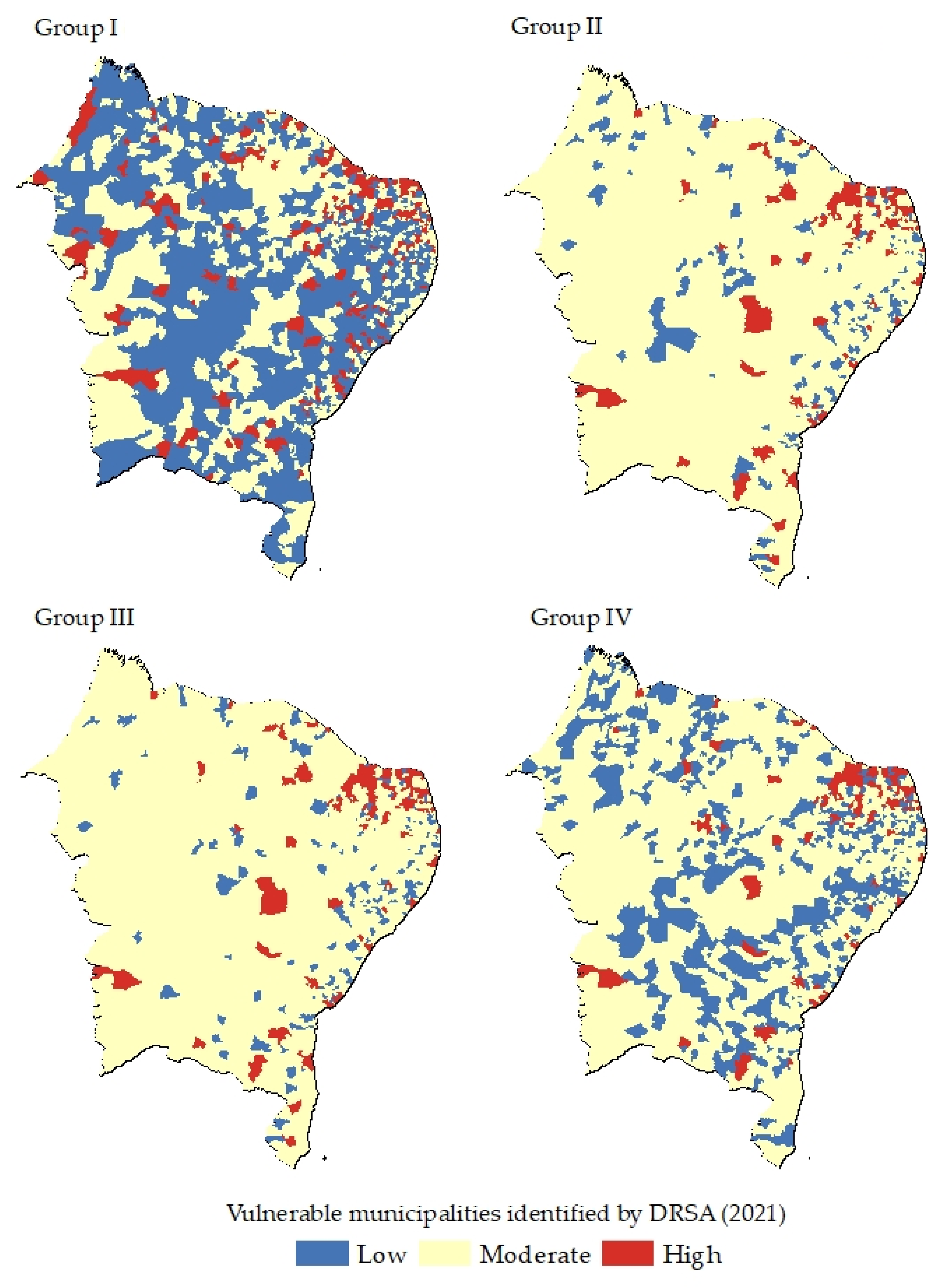
3.3. Multiple-Criteria Decision Model

We sought to classify the municipalities comprising Northeast Brazil in terms of vulnerability to COVID-19 according to the impact of multiple criteria that represent characteristics of these places. For this analysis, three categories representing vulnerability levels have been defined:

• Cl_Low—low vulnerability
• Cl_Moderate—moderate vulnerability
• Cl_High—high vulnerability

In this regard, we applied a method called dominance-based rough set approach (DRSA), which consists of exploring knowledge in a holistic manner based on inferences from previously known information [39]. The DRSA is a method for sorting problems using the non-classical multiple criteria decision approach [40].

Each application of the DRSA [39] is based on a data table formally represented by a four-tuple information system $S=\left\{A,Q,V,f\right\}$, where $A$ is a non-empty finite set of objects, and $Q$ is a non-empty finite set of attributes. The application of DRSA requires the establishment of a set of attributes and objects, with attribute $q\in Q$ and object $a\in A$. The $V_q$ is the domain of attributes $q$ and $V={{\displaystyle \cup }}_{q\in Q}{V}_q$, and $f:A\times Q\to V$ is a total function defined such that $f\left(a,q\right)\in V_q$ for each attribute $q\in Q$ and object $a\in A$. The set $Q$ is often divided into a subset $C=\left\{c_1,c_2,\dots ,c_m\right\}$ of condition attributes with $C\ne \varnothing$ and a subset $D\ne \varnothing$ of decision attributes, such that $C{\displaystyle \cup }D=Q$ and $C{\displaystyle \cap }D=\varnothing$. Moreover, reference objects consist of reference objects (or learning objects).

The DRSA is enriched by introducing an outranking relation ${\succcurlyeq }_c$ into $A^{*}$ with respect to the attribute $cϵC$, such that $a_1^{*}{\succcurlyeq }_c{a}_2^{*}$ means that $a_1^{*}$ is at least as good as $a_2^{*}$ with respect to attribute $c$.

For the sake of simplicity, in the following, we shall consider the case of a single decision attribute, i.e., $D=\left\{d\right\}$. More formally, let $Cl=\left\{C{l}_t,t\in \left\{1,\dots ,n\right\}\right\}$ be a set of classes of $A$ such that each $a_1^{*}\in A$ belongs to one and only one class $C{l}_t\in Cl$. Suppose $C{l}_r$ and $C{l}_s$ are two predefined classes with r, $s\in T$, $a_1^{*}\in C{l}_r,\mathrm{and}{a}_2^{*}\in C{l}_s$. If $r>s$, then $a_1^{*}\succcurlyeq a_2^{*}$. In this study, the set of decision class is represented by: $Cl=\{C{l}_{Low}>C{l}_{Moderate}>C{l}_{High}\}$.

The DRSA introduces the concept of an approximation of a set of objects (a union of decision classes) with respect to a set of attributes (or criteria). For $P\subseteq C$, the collection of all objects that can be classified into $C{l}_t^{\ge }$ that without any ambiguity constitutes the $P$-lower approximation of $C{l}_t^{\ge }$. The collection of all objects that could be classified into $C{l}_t^{\ge }$ constitutes the $P$-upper approximation of $C{l}_t^{\ge }$. Analogously, one can define the $P$-lower approximation of $C{l}_t^{\le }$ and the $P$-upper approximation of $C{l}_t^{\le }$.

For every $P\subseteq C$, the quality of approximation of the ordinal classification $Cl$ by the set of attributes is considered to be the ratio expressed by the cardinality between the universe $A$ and all $P$-correctly classified alternatives (Equation (2)).

$${\gamma }_P\left(Cl\right)=\frac{\left|A-\left({{\displaystyle \cup }}_{t=1,\dots ,n}B{n}_P\left(C{l}_t^{\le }\right)\right){\displaystyle \cup }\left({{\displaystyle \cup }}_{t=1,\dots ,n}B{n}_P\left(C{l}_t^{\ge }\right)\right)\right|}{\left|A\right|}$$

(2)

${\gamma }_P\left(Cl\right)$ can be seen as a degree of consistency of the objects from $A$, where $P$ is the set of attributes, and $Cl$ is the ordinal classification considered.

These approximations are explored to induce decision rules of the type “if …, then…” which are used to assign the objects into unions of classes $C{l}_t^{\ge }$ and $C{l}_t^{\le }$. Five types of decision rules may be considered [39], but we describe the rules used in the study as: i: certain $D_{\ge }$-decision rules generated from the lower approximation $\underset{\_}{P}(C{l}_t^{\ge })$; ii. certain $D_{\le }$-decision rules generated from $\underset{\_}{P}(C{l}_t^{\le })$.

The method creates a set of decision rules based on a training table and additionally, a training map. To build the table, we selected a subset of objects (called reference objects) to be assigned to only one class $C{l}_t$ according to its vulnerability level. All evaluations for choosing reference objects were made in the GIS environment to avoid the use of tables. To obtain the decision rules, DomLEM algorithms (Blaszczynski et al., 2013) were used.

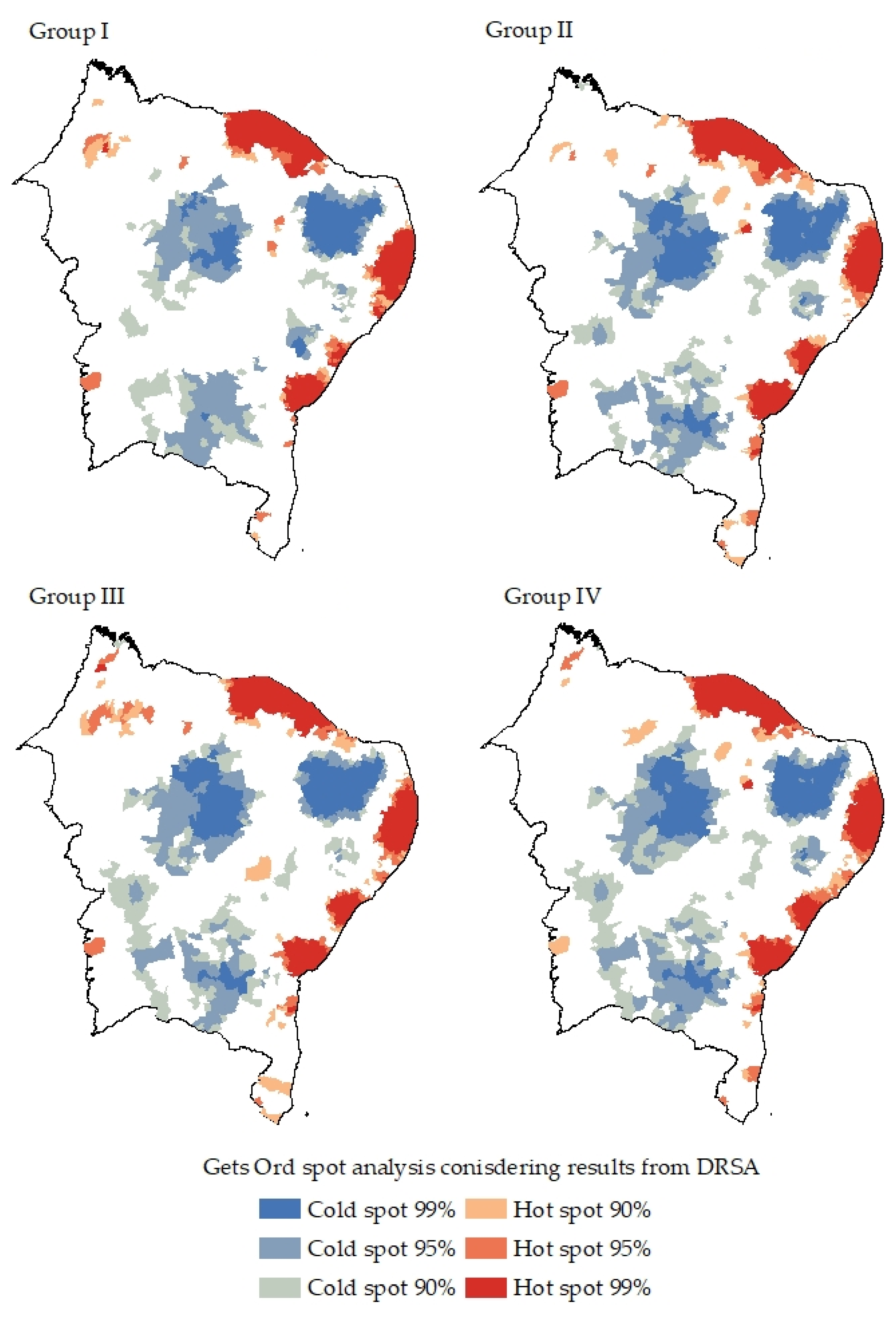
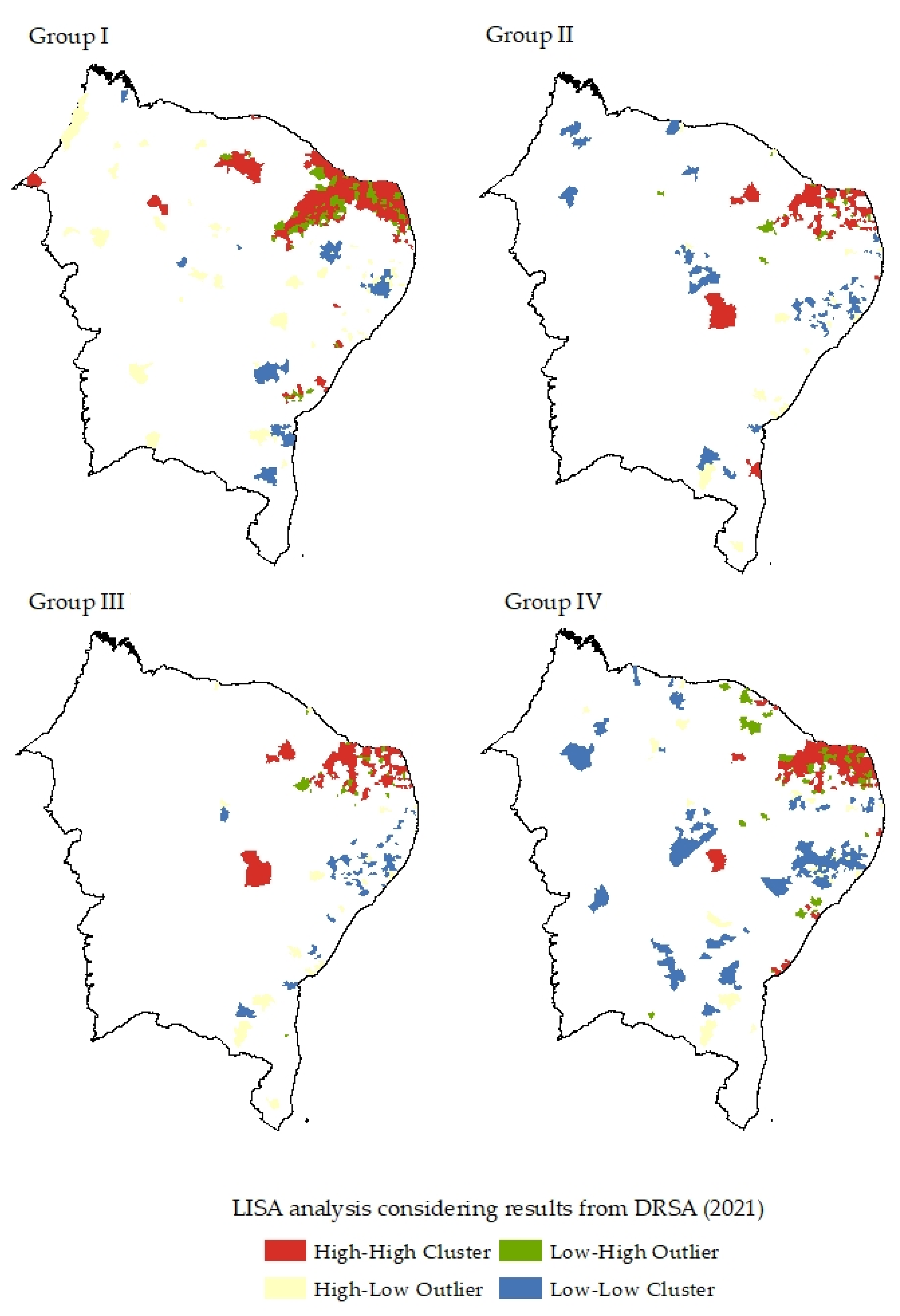
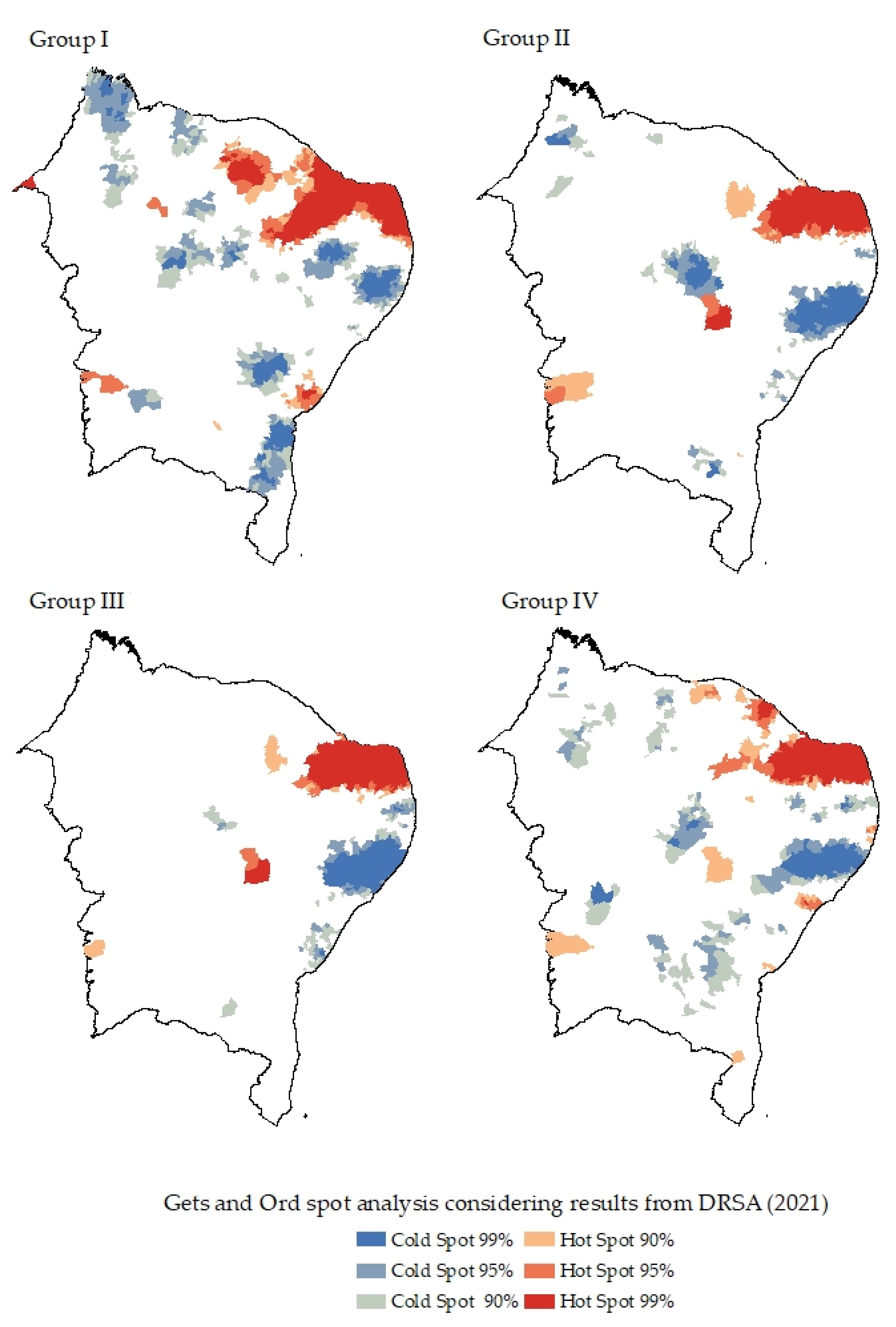
3.4. Spatial Inference

The last step comprised gathering the classification via the dominance-based rough set approach (DRSA), applying two spatial analyses, and identifying the cluster spatial classification. The Luc Anselin Local Moran’s I (LISA) [41], similar to the spatial analysis in step 3.2, was applied, except this method made it possible to locate and identify spatial clusters induced by other individual municipalities in global statistics and outlier evaluation. The statistical test sorted the clusters into four significant groups: clusters of high values (HH), clusters of low values (LL), outliers in which a high value is primarily surrounded by low values (HL), and outliers in which a low value is primarily surrounded by high values (LH). The index was obtained using Equation (3):

$$I=\frac{X_i-\overline{X}}{S_i^2}{{\displaystyle \sum }}_{j=1,j\ne i}^n{W}_{i,j}(X_j-\overline{X}),$$

(3)

where $X_i$ is an attribute for feature $i$, whereas $X_i$ is the mean of the corresponding attribute. $W_{i,j}$ is the spatial weight between feature $i$ and $j$, and $S_i^2$ is the standard deviation.

The second spatial statistic Getis and Ord ($G_{i^{*}})$ [38] is a measure of a statistical significance test related to clusters with high values (hot spots) and low values (cold spots), taking into account the sum of the performance for the area targeted in the study. The $G_{i^{*}}$ assay is a set of alternatives for measuring the degree of association of each performance to its neighborhood, to predefine distance. Equation (4) shows the calculation:

$$G_{i^{*}}=\frac{{{\displaystyle \sum }}_j{W}_{ij}\left(d\right)X_j}{{{\displaystyle \sum }}_j{X}_j}\mathrm{in}\mathrm{which}j\ne i,$$

(4)

where $X_j$ is the weight value for a given feature, and $W_{ij}\left(d\right)$ is a symmetric one/zero spatial weights matrix, with ones for all links defined as being within distance $d$ (or contiguous municipalities) of a given region $i$; all other links are zeros. In both cases (LISA, and Getis and Ord), the feature targets were considered based on the level of vulnerability to COVID-19 obtained in the previous DRSA step.

4. Results

As previously mentioned, this research was conducted to create a panel of associations regarding COVID-19 in the northeast region of Brazil. Figure 1 shows the nine federative units (Brazilian states) that constitute the northeast region (Figure 1b). Each of them has an administrative government and is composed of municipalities. The capital is the municipality where the head office of the state government is located. In total, there are 1793 municipalities in the nine states (Figure 1c). This region has approximately 57 million inhabitants, corresponding to 27.2% of the entire Brazilian population. The climate is semiarid in most areas, with drastic conditions (drought and rain scarcity) adversely affecting human development, agriculture, and the food industry [42,43]. Compared to other Brazilian regions, the northeast does not perform well in the socioeconomic index, unemployment, child mortality, and per-capita income, although industries have experienced significant growth in some areas [44]. Moreover, with regard to health infrastructures, its rural zones have a scarcity of medical supplies.

To conduct the experiments, we established four groups based on the selected features (outlined in Table 2), defining categories that involve social, economic, territorial, and demographic aspects. These groups were used to obtain and compare the results. Thereby, we referred to these groups as follows: Group I, Group II, Group III, and Group IV. The groups also include COVID-19 registries (daily case reports) as criteria to verify their impact on the quality of the extracted knowledge of the model, i.e., if/when the decision rules relay this information to obtain vulnerability classification. With regard to the period outbreak, three different days were chosen with peaks of COVID-19 cases registered in the Brazilian northeast counties. The variables created (Area 1, Area 2, Den 1 and Den 2) were included in all groups too due to the importance of characterizing the geographic spaces of the counties. The groups were defined as follows: Group I was considered as the “group control” (all variables). The other groups were divided by similar characteristics.

Table 3. Groups and variables.

Variable	Group I	Group II	Group III	Group IV
Pop_estim	**	**		**
Peop_ocup	**		**	**
Income_m	**		**
Pop_ocu	**	**	**
Income_prop	**		**
Esco_1	**
Esco_2	**
MHDI	**	**	**	**
GPD	**	**	**	**
Schollar_prop	**
SUS	**
Sewage	**
Area	**	**	**	**
Area1	**	**	**	**
Area2	**	**	**	**
Den	**	**	**	**
Den1	**	**	**	**
Den2	**	**	**	**
Day_1 (06/24)—2020	**	**	**	**
Day_2 (06/27)—2020	**	**	**	**
Day_3 (06/30)—2020	**	**	**	**

** criteria used for each group.

shows the features of each group, whereas

Table 4. Descriptive features.

Variable	Mean	Min	Max	SD
Pop_estim	31,813	1246	2,872,347	119,072
Peop_ocup	5295	59	849,711	37,919
Income_m	1.80	0.80	6.50	0.37
Pop_ocu	8.94%	1.00%	79.40%	5.59%
Income_prop	51.54%	22.70%	64.10%	4.84%
Esco_1	28	1	1173	53
Esco_2	4	0	307	14
MHDI	0.591	0.443	0.788	0.043
GPD	11,207.52	3285.04	253,895.58	11,181.27
Schollar_prop	97%	81%	100%	2%
SUS	12	1	367	19
Sewage	25.37%	0.00%	97.30%	22.09%
Area	865.20	18.61	15,634.33	1355.32
Area1	12.73	0.18	421.88	29.89
Area2	6.66	0.06	293.36	17.67
Den	98.27	0.84	9503.20	456.85
Den1	3681.23	202.18	39,399.11	2930.72
Den2	6357.30	281.86	122,002.24	6861.10

Max: maximum value; Min: minimum value; SD: standard deviation.

presents the descriptive data.

The evolution of COVID-19 records followed the expected trend, with rapid spread in urban centers and later, contagion in small and medium municipalities. Small municipalities have few medical resources, and any sudden new cases alerted the local health service capacities. On the other hand, small cities also have low population densities, which probably reduced the chances of contagion.

Over the months that were analyzed, we observed spatial statistical significance among the COVID-19 records in the northeast region (

Table 5. Spatial autocorrelation observed for several days.

Date (DD-MM)	15-03	30-03	15-04	30-04	15-05	30-05	15-06	30-06
Moran’s index	0.000152	0.000012	0.000470	0.001537	0.002523	0.004999	0.006344	0.006194
z-score	0.583468	0.649571	0.954859	1.726499	2.568552	4.373238	5.183223	4.957213
p-value	0.559579	0.515969	0.339649	0.084258	0.010212	0.000012	0.000	0.0000
Model	Random	Random	Random	Clustered	Clustered	Clustered	Clustered	Clustered

). On the first three dates (15 March, 30 March, and 15 April 2020), no statistical significance was observed among the records assigned by Global Moran’s I as random events. Nonetheless, from 30 April, significance was observed for the cluster pattern. This finding is explained by the high numbers of records for urban centers and around cities.

The groups selected for the experiments were then analyzed for correlations of features and reference days (30 June 2020) (

Table 6. Statistical correlation and OLS used on the groups.

Group	OLS
	Adjusted R2	AICc	p-Value
Group I	0.95	26,186.30	0.0000
Group II	0.93	26,366.51	0.0000
Group III	0.93	26,450.05	0.0000
Group IV	0.051	28,178.83	0.0000

), obtaining a highly explanatory statistical power (adjusted R2 above 90%), except for Group IV. The results in terms of AIC are close with a significant correlation (p-value). Thus, the proposal to use the four groups as separate sets of attributes to evaluate reference objects (municipalities) is attractive and allows for the following step of using DRSA to explore decision rules.

In the third step, we applied DRSA aiming to explore its resulting decision rules. For each group, we retried the reference object and established the decision class based on 30 June 2020 as the reference day. The records were observed in groups of 100 thousand inhabitants, which were divided according to Jenks natural breaks algorithm. This method helped to classify the feature target (COVID-19 cases) based on the best sorting arrangement, aiming to reduce variance inside each class and maximize the variance between classes. Afterward, we retried the decision-maker procedure to select the remaining decision classes. Figure 2 represents accumulated data of COVID-19 confirmed cases until 30 June 2020, sorted by natural breaks. These results were used to build the reference objects.

A randomized procedure was performed to select reference objects, and each object was assigned a decision class: $Cl=\{C{l}_{Low}>C{l}_{Moderate}>C{l}_{High}\}$. The decision classes represent the three levels of vulnerability related to COVID-19. With the support of the results from Figure 2, a holistic analysis was performed to assign each selected reference object for all groups (I, II, III, and IV). The procedure allows the extraction of strong information about which criteria may represent the knowledge for classification, providing decision rules (If… Then… $Cl$).

Furthermore, for all groups, the same sets of objects were considered, varying only the attributes for each group. There were 18 objects for the high vulnerability level, 47 for the moderate vulnerability level, and 116 for the low vulnerability level, which results in a total of 181 objects to gather decision rules. For all groups, the following DRSA parameters were analyzed: quality of approximation, reducts, and core (

Table 7. Parameters generated via DRSA in relation to reference objects.

Group	Reducts	Core	Quality
Group I	4	Esco, sewage, area, den	0.989
Group II	4	Pro_ocup, MHDI, area, den, den1, c3006	0.901
Group III	7	Income_m, MHDI, area, den, den1, c3006	0.917
Group IV	1	Peop_ocup, MHDI, GPD, area, den, den1, den2, c2406, c3006	0.901

).

The exception among the groups was Group IV, for which only one reduct was obtained. By comparison, at least four reducts were obtained for each of the other groups. This result indicates that for Group IV, information can be observed based only on attributes of that reduct. With regard to the cores, the intersections between the reducts were attributed to population (density), economic aspects (gross domestic product and income), and municipality area. In contrast with Group I, the COVID-19 registries were often observed for Groups II, III, and IV. All groups had qualities of approximation that were above 0.90, although the consistency of representation was maintained.

A separate analysis in groups (Group I to IV) is justified due to the advantage of revealing different sets of attributes and different features, with good quality of approximation. Having different set of features allows the generation of and, somehow, the comparison of decision rules and patterns of vulnerability that is useful for decision making. Furthermore, holistic decision-making models require prior knowledge (preferential knowledge) that might be difficult to assess when there are a high number of attributes. Studies of biases in decision making show that when there is too much information, the human mind tends to focus on a subset of information to make judgments [45]. Although the DRSA is able to reduce the number of attributes, it is desirable to explore different subsets of attributes leading to similar results.

Subsequently, the decision rules that were obtained served to classify the entire set of municipalities and compare the results obtained with each group of criteria. According to experiments using DRSA, the vulnerability levels in terms of all Group I attributes could be represented by 62 decision rules and in Group II by 58, whereas Groups III and IV each produced 56 rules. The difference in the number of decision rules among groups was a consequence of being proportional to the quantity of both reference objects and attributes used. With regard to the types of union approximation class (At Least and At Most), the ones that prevailed were At Most 1, At Most 2, and At Least 3 also because of the number of reference objects for each class.

Table 8. Sample of decision rules obtained from DRSA.

Group	Rules
Group I	IF pop_estim >= 42,130.0 AND esco <= 0.926 THEN At Least 3 IF sewage <= 0.377 AND area >= 567.78 AND den >= 68.225369 THEN At Least 3 IF Income_m >= 1.7 AND c3006 >= 8.0 THEN At Least 2 IF pop_estim >= 28,933 AND esco <= 0.959 THEN At Least 2 IF ocup_mei >= 0.539 AND den <= 17.578066 THEN At Most 1 IF Peop_ocup <= 463.0 AND den <= 30.431274 THEN At Most 1 IF mhdi <= 0.548 AND c2706 <= 9 THEN At Most 2 IF Peop_ocup <= 862.0 AND c2706 <= 0 THEN At Most 2	C: 90.05 I: 9.95
Group II	IF area >= 270.752 AND c2706 >= 50.0 AND c3006 >= 20.0 THEN At Least 3 IF area >= 842.106 AND c3006 >= 22 THEN At Least 3 IF den >= 124.146236 AND den2 <= 10,760.08 THEN At Least 2 IF pop_estim >= 28,933.0 AND mhdi >= 0.592 AND den >= 88.545652 THEN At Least 2 IF pib <= 51,697.69 AND den <= 13.66 THEN At Most 1 IF pro_ocup <= 0.054 AND c2706 <= 2 THEN At Most 1 IF mhdi <= 0.534 THEN At Most 2 IF area2 <= 1.88 AND c3006 <= 7 THEN At Most 2	C: 90.05 I: 9.95
Group III	IF area >= 270.752 AND c2706 >= 50 AND c3006 >= 20 THEN At Least 3 IF area >= 755.59 AND c2706 >= 37 THEN At Least 3 IF pib >= 25,892.88 AND den >= 19.24 THEN At Least 2 IF area2 >= 4.24 AND c2406 >= 7 THEN At Least 2 IF Peop_ocup <= 421 AND pib <= 7434.96 THEN At Most 1 IF Income_m <= 1.7 AND den <= 19.593458 AND den2 >= 16,998.68 THEN At Most 1 IF den <= 17.57 AND c2406 <= 14 THEN At Most 2 IF mhdi <= 0.548 AND c2706 <= 9 THEN At Most 2	C: 88.40 I: 11.60
Group IV	IF area >= 270.752 AND c2706 >= 50 AND c3006 >= 20 THEN At Least 3 IF area >= 385.583 AND c2406 >= 16 AND c3006 >= 24 THEN At Least 3 IF den1 <= 493.20 THEN At Least 2 IF den >= 124.14 AND den2 <= 10,760.08 THEN At Least 2 IF mhdi <= 0.534 AND pib <= 6811.66 THEN At Most 1 IF pib <= 11,566.03 AND den <= 19.59 AND den2 >= 16,998.68 THEN At Most 1 IF den1 >= 7400.67 THEN At Most 2 IF area2 <= 2.17 AND den <= 73.11 AND c3006 <= 2 THEN At Most 2	C: 89.50 I: 10.50

presents a sample of the decision rules for each group.

Figure 3 shows the results of the classification of all municipalities in terms of vulnerability to COVID-19 cases, considering the decision rules from DRSA. Each map is associated with the reference objects groups that were used. Strong similarities between the groups were verified, and, in all of them, there was a high prevalence of the low and moderate vulnerability levels, besides a few distinguished the high vulnerability level areas. In general, the results remain similar even when changes in attributes were applied. There were small variations within groups in municipalities between low and moderate vulnerability classes, whereas, between groups, few municipalities were considered to be of high vulnerability in some groups and of moderate vulnerability in others. We observed that almost all coastal zones were revealed to be moderately vulnerable to COVID-19, where the populations are higher than in the inside zones.

In relation to the COVID-19 cases registered on the three days used as input in the model, our findings confirm such features contribute to obtaining satisfactory results. Observing the results on the four groups (Figure 3) and density accumulated cases (Figure 2), there is a pattern around the distribution at the classes. There are concentrations of one of type of classification pattern on the littoral zone (moderate vulnerability), and on the inside of the map, there are other pattern classification types (low vulnerability).

The fourth step of modelling consisted of exploring the spatial clusters sourced from DRSA, applying two techniques widely discussed in the literature: LISA, and Getis and Ord ($G_{i^{*}}$). Both methods locate the cluster formations taking into account the feature target, which was the vulnerability classification measures obtained from DRSA. Figure 4 and Figure 5 present the results, distinguishing the nature of each cluster. The purpose of the clusters is to identify the concentration of decision classes from Figure 3.

The LISA approach identified four types of regions (clusters and outliers). HH clusters were most evident for coastal zones, where municipalities have similar classifications. On the other hand, HL municipalities indicated moderate and high vulnerability levels, involving dissimilarities among the alternatives. Finally, LH and LL were less highlighted than the other clusters. Meanwhile, analysis using Getis and Ord ($G_{i^{*}}$) resulted in other cluster formations but had similar results compared to those of LISA. The results show more concentrated clusters (hot and cold formations). An analogous zone of similar classifications was also revealed for the coastal regions.

The validation procedure consisted of an exploration of a new analysis to identify vulnerable places for COVID-19 at the final second outbreak phase (2021). For the new analysis, a change was implemented: registered COVID-19 cases were used as input to create decision rules whilst maintaining the other criteria (

Table 9. Parameters generated via DRSA in relation to reference objects in 2021.

Group	Reducts	Core	Quality
Group I	1	Income_m, pro_ocup, ocup_mei, MHDI, pib, esco, sewage, area, den, den1, den2, c2206, c2606	0.872
Group II	1	Pro_ocup, odhm, pib, area, den, den1, den2, c2206, c2406, c2606	0.739
Group III	1	Income_m, prop_ocup, ocup_mei, MHDI, pib, area, den, den1, den2, c2206, c2406, c2606	0.789
Group IV	1	Mhdi, pib, area, den, den1, den2, c2206, c2406, c2606	0.722

). The objective was to check if it was possible to accurately identify vulnerable areas by only uploading data from new, registered COVID-19 cases. The analysis was again performed for the four groups considered, and the days chosen were: 22 June, 24 June, and 26 June. For the northeast Brazilian region, 69,038 cases were registered on 22 June, and 17,051 on 24 June. On 24 June, there were 11,499 COVID-19 cases officially confirmed. To provide the new results, we included 180 reference objects to perform the second analysis, excluding the registers applied on the 2020 analysis. The reference objects were also changed to verify the quality of information used. The quality of reference objects presented small fluctuations when observed between the groups. In relation to the number of “Reducts” and “Core” obtained from the DRSA approach, the values were the same for all. Notably, the quality decreased for all groups compared to the reference objects used in 2020. However, with this same parameter above 70%, we can keep the objects with existing evidence and continue to use the data to obtain the decision rules.

The vulnerable municipalities identified on the second analysis revealed more “High vulnerability class” in comparison with the 2020 results (Figure 6). Considering the sum for the three days, in 2021, a total of 97,588 cases occurred, while, in 2020, there were 41,318 cases. If we compare Figure 3 to Figure 6, 2020 has more municipalities sorted as “Low”, while, in 2021, there were more municipalities allocated to the moderate and high classes. It can be seen that only updating the cases registered is necessary to reveal the vulnerable municipalities. In relation to the groups in 2021, the results achieved for Group I show more municipalities allocated to the low vulnerable classification than other groups. The Group II and Group III have similarities in classes. In Group IV, their contiguous surfaces are classified as low, moderate, and high vulnerabilities. We highlight that the municipalities that are more vulnerable (high) are closer between Groups II, III, and IV than the results shown for Group I.

Table 10. Distribution of municipalities for the vulnerable classes for groups observed in 2020 and 2021.

	Group I		Group II		Group III		Group IV
Year	2020	2021	2020	2021	2020	2021	2020	2021
High	22	209	15	104	11	109	16	100
Moderate	461	549	554	1532	561	1537	578	1149
Low	1311	1035	1225	544	1222	147	1200	544

summarizes both results.

Figure 7 and Figure 8 show the distribution of the classification with regards to the spatial analysis clusters used (LISA, and Getis and Ord). According to LISA analysis, the concentration of high-high municipalities were associated in the same positions as the municipalities classified as showing a high vulnerability. We observed that, for Group I, there were more clusters formed than the other groups due the variability of information. In addition, the high concentration clusters presented as high-high in the northeast sector of the figure contrast with municipalities allocated as low-high. Moreover, there is an important detail present in the results obtained from the LISA analysis: all groups (I, II, III, and IV) have the presence of municipalities allocated as low-low which means more registered cases concentrated in few places. In fact, in 2020, the ten first municipalities with more cases represented 44% of the cases of the total registers in the northeast Brazilian region, while, in 2021, the ten top municipalities represented 53% of total registers. The results achieved by Getis and Ord show similar concentration when compared to the LISA results but include information related to the cold clusters, allowing a deep analysis of the less vulnerable (low class) of municipalities. Finally, in both results, in the Rio Grande do Norte (RN) state, there are concentrated regions marked as high-high (LISA) and hot spots with 99% significance (Getis and Ord). On the three days analyzed, this state represented 59% of all the cases registered.

We also compared the criteria resulting from assignments given by the application of decision rules induced on reference objects and the number of rules created.

Table 11. Criteria used on decision rules for groups in 2020 and 2021.

Groups	2020	2021
Group I	#62 Den, den1, den2, pop_ocup, GPD, MHDI, sewage, Schollar_prop, Esco_1, area, June days 2020 (24; 27; 30)	#96 MHDI, den1, den2, income_m, peop_ocup, area, sewage, June days 2021 (22; 24; 26)
Group II	#58 Den, den1, MHDI, area, GPD, income_prop, pop_estim, June days 2020 (24; 27; 30)	#50 Area, pop_ocup, MHDI, GPD, den, den1, den2, June days 2021 (22; 24)
Group III	#56 Area, den1, den2, MHDI, peop_ocup, MDHI, June days 2020 (24; 27)	#52 Area, income_m, MHDI, den2, income_prop, GPD, income_m, June days 2021 (22; 24)
Group IV	#56 Sewage, income_m, area, pop_ocup, den, den2, GPD, income_prop, MHDI, June days 2020 (24; 27)	#47 Area, den1, den2, GPD, MHDI, June days 2021 (24; 22)

describes the criteria used to create the decision rules. It is fruitful to note that the criteria considered were essential to identify vulnerable places, as well as employing registered cases as criteria. Concerning the criteria used to perform vulnerability classification, we confirm that the model is suitable to employ several related factors: social, economic, and demographics. In addition, aspects related to population, density population, and income have a deep impact because they are associated with the movement of people in urbans areas. Indirectly, other aspects (GPD and sewage) could be used to support decisions. Therefore, based on both results, we judge that the methodology for COVID-19 used here has great potential to help policies planners to make public decisions.

The outbreak of the COVID-19 pandemic has spurred the emergence of a broad field of research about the virus and the factors associated with its spread. The study presented in [14] showed similar patterns assigned with high density counties (the virus spread faster than small counties). However, large cities also must not be seen as at risk to maximum exposure COVID-19, highlighting that, in these cities, there are more facilities available [15]. For instance, Brazil has presented a gap in hospital units available in small cities, which has led to patients being transported to the capital of the states [16]. Moreover, our study contributes to the identification of characteristics such as population density, income, and the size of counties associated with the measure of the vulnerability level. As a consequence, such aspects must be considered when making decisions related to the prevention of the disease and the mitigation of registered cases.

5. Discussion and Final Remarks

We introduce a model capable of revealing the main attributes and conditions that characterize municipalities in relation to levels of vulnerability. The model is able to identify the main municipalities vulnerable to COVID-19, integrating several methods based on spatial analysis and multiple-criteria decision making. Northeast Brazil was the region examined and on which the model was demonstrated. Firstly, a set of attributes was selected for evaluation along with daily recorded cases. Spatial analysis techniques and DRSA were then used for data treatment and the measurement of vulnerability, respectively. Afterward, two expressive cluster analyses were performed, showing several hot spot areas based on the DRSA results. To create a comprehensive model, we applied new reference objects to June 2021 to check the accuracy the model, considering the increase in occurrences.

The DRSA method is a holistic approach that maintains the quality of information, taking into account essential attributes. It also returns decision rules which helped to reveal distinctive patterns among municipalities that make them alike concerning the spread of COVID-19. Accordingly, the methodology was particularly useful for exploring the data in our study. The classification (measure of vulnerability) is the result of the observation of four main aspects: social, economic, demographic, and territorial. We conclude that population, gross domestic product, income, and population density are important characteristics for identifying which cities may require further investigation. In addition, these same variables contribute to classification into moderate and low vulnerability levels. On the other hand, daily COVID-19 records, population density, and territorial area are the most important for the entire classification. Nevertheless, the DRSA method based on four distinct groups of attributes is able to evaluate both the small and large cities in the northeast region of Brazil.

In relation to cluster analysis, a search for places with similar vulnerability levels was performed. As a consequence, it simplified the comprehension about which areas require the same (or even opposite) harshness of administrative measures to prevent the spread of the disease. Moreover, the findings of our study are similar to those of other studies, since we demonstrated that urban centers have a greater propensity to disseminate the virus and are more affected by it. However, this information is not limited to large urban zones; rural zones were also evaluated. The findings of this research may support several public policies on health assistance to alleviate the adverse consequences of COVID-19.

In a pandemic context, the findings here serve to tell the trajectory of the COVID-19 cases in urban and rural places beyond the variables associated with the cases registered. To achieve the answers across maps in [46], visualizations bring several benefits to the understanding of the effect on society and economy, for example. Regarding the spread and dissemination of the virus, our study revealed a strong concentration of cases in metropolitan areas around the administration of capital states, with similar results found in [14,31]. It does not occur as a random event, but the places are connected to each other [47].

The variables used here (demographic density, area, income, and daily cases) give crucial insights to aspects about spatial analysis (OLS), and the results from DRSA might also be used by spatial analysis (LISA, and Getis and Ord hot spot). Our results align with similar results that used social and inequality variables with regards to COVID-19 and show how these variables achieve important results related to spatial inferences [25,26,30]. In addition, the spatial dimension using a large space (the Brazilian northeast) reveals how small towns even classified as showing high vulnerability or moderate vulnerability are isolated precisely because they are not connected to associated urban spaces.

Finally, the contribution of this study consists in associating several factors (socioeconomic, demographic, and territorial) with COVID-19, specifically in Brazilian regions. The proposed method would be useful for performing vulnerability evaluation and for guiding decision makers. However, we also have to address some limitations, such as the consideration of update data and other features regarding the municipalities for further analysis, which may be explored in future research.

References

1. Guan, W.; Ni, Z.; Hu, Y.; Liang, W.; Ou, C.; He, J.; Liu, L.; Shan, H.; Lei, C.; Hui, D.; et al. Clinical Characteristics of Coronavirus Disease 2019 in China. N. Engl. J. Med. 2020, 382, 1708–1720. [Google Scholar] [CrossRef] [PubMed]
2. Zhou, P.; Yang, X.L.; Wang, X.G.; Hu, B.; Zhang, L.; Zhang, W.; Si, H.R.; Zhu, Y.; Li, B.; Huang, C.L.; et al. Pneumonia outbreak associated with a new coronavirus of probable bat origin. Nature 2020, 579, 270–273. [Google Scholar] [CrossRef] [PubMed]
3. Gorayeb, A.; de Oliveira Santos, J.; da Cunha, H.G.; da Silva, R.B.; de Souza, W.F.; Mesquita, R.D.; da Silva Libério, L.; de Sousa Silva, F.D.; do Nascimento, S.L.; Mota, C.M.; et al. Volunteered Geographic Information Generates New Spatial Understandings of COVID-19 in Fortaleza. J. Lat. Am. Geogr. 2020, 19, 260–271. [Google Scholar] [CrossRef]
4. Coelho, F.C.; Lana, R.M.; Cruz, O.G.; Villela, D.A.; Bastos, L.S.; Pastore y Piontti, A.; Davis, J.T.; Vespignani, A.; Codeço, C.T.; Gomes, M.F. Assessing the spread of COVID-19 in Brazil: Mobility, morbidity and social vulnerability. PLoS ONE 2020, 15, e0238214. [Google Scholar] [CrossRef] [PubMed]
5. COVID-19 Dashboard by the Center of Systems Science and Engineering (CSSE) at Johns Hopkins University (HUI). Coronavirus Resrouce Center = Johns Hopkins University & Medicine. [Online]. Available online: https://coronavirus.jhu.edu/map.html (accessed on 25 March 2022).
6. Freitas, C.M.; Silva, I.V.M.; Cidade, N.C. COVID-19 as a global disaster: Challenges to risk governance and social vulnerability Brazil. Rev. Ambiente Soc. 2020, 23, 1–12. [Google Scholar] [CrossRef]
7. Ribeiro, H.V.; Sunahara, A.A.; Sutton, J.; Perc, M.; Hanley, Q.S. City size and the spreading of COVID-19 in Brazil. PLoS ONE 2020, 15, e0239699. [Google Scholar] [CrossRef]
8. Braga, J.U.; Ramos, N.A.; Ferreira, A.F.; Lacerda, V.M.; Freire, R.M.C.; Bertoncini, B.V. Propensity for COVID-19 severe among the populations of the neighborhoods of Fortaleza, Brazil, in 2020. BMC Public Health 2020, 20, 1486. [Google Scholar] [CrossRef]
9. Marson, F.A.L. COVID-19-6 milion cases worldwide and an overview of the diagnosis in Brazil: A tragedy to be announced. Diagn. Microbiol. Infect. Dis. 2020, 98, 115113. [Google Scholar] [CrossRef]
10. Nepomuceno, T.C.C.; Silva, W.M.N.; Nepomuceno, K.T.C.; Barros, I.K.B. A DEA-Based Complexity of Needs Approach for Hospital Beds Evacuation during the COVID-19 Outbreak. J. Healthc. Eng. 2020, 2020, 8857553. [Google Scholar] [CrossRef]
11. Ferraz, F.D.; Mariano, E.B.; Manzine, P.R.; Moralles, H.F.; Morceiro, P.C.; Torres, B.G.; de Almeida, M.R.; Soares de Mello, J.C.; Rebelatto, D.A.D.N. COVID Health Structure Index: The vulnerability of Brazilian Microregions. Soc. Indic. Res. 2021, 159, 197–215. [Google Scholar] [CrossRef]
12. Huang, Q.; Jackson, S.; Derakhshan, S.; Lee, L.; Pham, E.; Jackson, A.; Cutter, S.L. Urban-rural differences in COVID-19 exposures and outcomes in the South: A preliminary analysis of South Carolina. PLoS ONE 2020, 16, e0246548. [Google Scholar] [CrossRef] [PubMed]
13. Markovc, R.; Sterk, M.; Marhl, M.; Perc, M.; Gosak, M. Socio-demographic and health factors drive the epidemic progression and should guide vaccination strategies for best COVID-19 containment. Results Phys. 2021, 26, 104433. [Google Scholar] [CrossRef] [PubMed]
14. McMahon, T.; Chan, A.; Havlin, S.; Gallos, L.K. Spatial correlations in geographical spreading of COVID-19 in the United States. Sci. Rep. 2022, 12, 699. [Google Scholar] [CrossRef] [PubMed]
15. Khavarian-Garmsir, A.; Sharifi, A.; Moradpour, N. Are high-density districts more vulnerable to the COVID-9 pandemic? Sustain. Cities Soc. 2021, 70, 102911. [Google Scholar] [CrossRef]
16. Nicolelis, M.; Raimundo, R.L.G.; Peixoto, P.S.; Andre, C.S. The impact of super-spreader cities, highways, and intensive care availability in the early stges of the COVID19 epidemic in Brazil. Sci. Rep. 2021, 11, 13001. [Google Scholar] [CrossRef]
17. Scarpone, C.; Brinkmann, S.T.; Grobe, T.; Sonnenwald, D.; Fuchs, M.; Walker, B.B. A multimethod approach for county-scale geospatial analysis of emerging infectious diseases: A cross-sectional case study of COVID-19 incidence in Germany. Int. J. Health Geogr. 2020, 19, 32. [Google Scholar] [CrossRef]
18. Han, Y.; Yang, L.; Jia, K.; Li, J.; Feng, S.; Chen, W.; Zhao, W.; Pereira, P. Spatial distribution characteristics of the CVODI-19 pandemic in Beijing and its relationship with environmental factors. Sci. Total Environ. 2021, 761, 144257. [Google Scholar] [CrossRef]
19. Fall, E.S.; Abdalla, E.; Quansah, J.; Franklin, M.J.; Whaley-Omidire, W. County-level assessment of vulnerability to COVID-19 in Alabama. ISPRS Int. J. Geo-Inf. 2022, 11, 320. [Google Scholar] [CrossRef]
20. Sharma, S.N.; Basu, S.; Sharma, P. Sociodemographic determinants of the adoption of a contact tracing application during the COVID-19 epidemic in Delhi, India. Health Policy Technol. 2021, 10, 100496. [Google Scholar] [CrossRef]
21. Andersen, L.M.; Harden, S.R.; Sugg, M.M.; Runkle, J.D.; Lundquist, T.E. Analyzing the spatial determinants of local COVID-19 transmission in the United States. Sci. Total Environ. 2021, 754, 142396. [Google Scholar] [CrossRef]
22. Ma, J.; Zhu, H.; Li, P.; Liu, C.; Li, F.; Luo, Z.; Zhang, M.; Li, L. Spatial patterns of the spread of the COVID-19 in Singapore and the influencing factors. ISPRS Int. J. Geo-Inf. 2022, 11, 152. [Google Scholar] [CrossRef]
23. Penha, M.E.R. The pandemic and its ethno-spatial disparities: Considerations from Salvador, Bahia, Brasil. J. Lat. Am. Cult. Stud. 2020, 29, 325–331. [Google Scholar] [CrossRef]
24. Maciel, J.A.C.; Castro-Silva, I.I.; Farias, M.R. Analise inicial da correlação espacial entre a incidência de COVID-19 e o desenvolvimento humano nos municípios do estado do Ceará no Brasil. Rev. Bras. De Epidemiol. 2020, 23, e200057. [Google Scholar] [CrossRef] [PubMed]
25. Paula, D.P.; Medeiros, D.H.; Barros, E.L.; Guerra, R.G.; Santos, J.D.; Lima, J.S.; Monteiro, R.M. Diffusion of COVID-19 in the Northern Metropolis in Northeast Brail: Territorial dynamics and risks associated with Social Vulnerability. Soc. Nat. 2020, 32, 639–656. [Google Scholar] [CrossRef]
26. Souza, A.P.G.; Mota, C.M.M.; Rosa, A.G.F.; Figueiredo, C.J.J.; Candeias, A.L.B. A spatial-temporal analysis at the early stages of the COVID-19 pandemic and its determinants: The case of Recife neighborhoods, Brazil. PLoS ONE 2022, 17, e0268538. [Google Scholar] [CrossRef]
27. Natividade, M.D.S.; Bernardes, K.; Pereira, M.; Miranda, S.S.; Bertoldo, J.; Teixeira, M.D.G.; Livramento, H.L.; Aragão, E. Social distancing and living conditions in the pandemic COVID-19 in Salvador-Bahia, Brazil. Ciênc. Saúde Coletiva 2020, 25, 3385–3392. [Google Scholar] [CrossRef]
28. Silva, A.P.S.C.; Maia, L.T.S.; Souza, W.V. Severe acute respiratory syndrome in Pernambuco: Comparison of patterns before and during the COVID-19 pandemic. Ciênc. Saúde Coletiva 2020, 25, 4141–4150. [Google Scholar] [CrossRef]
29. Brito, P.L.; Kuffer, M.; Koeva, M.; Pedrassoli, J.C.; Wang, J.; Costa, F.; Freitas, A.D. The spatial dimension of COVID-19: The potential of earth observation data in support of slum communities with evidence from Brazil. ISPRS Int. J. Geo-Inf. 2020, 9, 557. [Google Scholar] [CrossRef]
30. Tang, I.W.; Vieira, V.M.; Shearer, E. Effect of socioeconomic factors during the early COVID-19 pandemic: A spatial analysis. BMC Public Health 2022, 22, 1212. [Google Scholar] [CrossRef]
31. Ramírez, I.J.; Lee, J. COVID-19 emergence and social and health determinants in Colorado: A rapid spatial analysis. Int. J. Environ. Res. Public Health 2020, 17, 3856. [Google Scholar] [CrossRef]
32. Mota, C.M.M.; Figueiredo, C.J.J.; Pereira, D.V.S. Identifying areas vulnerable to homicide using multiple criteria analysis and spatial analysis. Omega 2021, 100, 102211. [Google Scholar] [CrossRef]
33. Gao, Z.; Jiang, Y.; He, J.; Wu, J.; Xu, J.; Christakos, G. An AHP-based regional COVID-19 vulnerability model and its application in China. Model. Earth Syst. Environ. 2022, 8, 2525–2538. [Google Scholar] [CrossRef] [PubMed]
34. Malakar, S. Geospatial modelling of COVID-19 vulnerability using an integrated fuzzy MCDM approach: A case study of West Bengal, India. Model. Earth Syst. Environ. 2021, 27, 1–14. [Google Scholar] [CrossRef] [PubMed]
35. Yetim, B.Y.; Sönmez, S.; Konca, M.; Ilgun, M. Prioritization of the policies and practices applied in Turkey to fight against COVID-19 through AHP technique. Saúde Soc. 2021, 30, 1–11. [Google Scholar] [CrossRef]
36. Sarkar, S.K. COVID-19 susceptibility mapping using multicriteria evaluation. Disaster Med. Public Health Prep. 2021, 14, 521–537. [Google Scholar] [CrossRef] [PubMed]
37. Brazilian Institute of Geography and Statistics. IBGE Cidades IBGE. 2020. Available online: https://cidades.ibge.gov.br/ (accessed on 21 January 2021).
38. Getis, A.; Ord, J.K. The Analysis of Spatial Association by Use of Distance Statistics. Geogr. Anal. 1992, 24, 189–206. [Google Scholar] [CrossRef]
39. Greco, S.; Matarazzo, B.; Slowinski, R. Rough sets methodology for sorting problems in presence of multiple attributes and criteria. Eur. J. Oper. Res. 2002, 138, 247–259. [Google Scholar] [CrossRef]
40. Alvarez, P.A.; Ishizaka, A.; Martínez, L. Multiple-criteria decision making sorting methods: Survey. Expert Syst. Appl. 2021, 183, 115368. [Google Scholar] [CrossRef]
41. Anselin, L. Local Indicators of Spatial Association–LISA. Geogr. Anal. 1995, 27, 93–115. [Google Scholar] [CrossRef]
42. Brasil, P.; Medeiros, P. NetStRes–Model for Operation of Non-Strategic Reservoirs for irrigation in drylands: Model descrition and application to a semiarid basin. Water Resour. Manag. 2020, 34, 195–210. [Google Scholar] [CrossRef]
43. Haguenauer, H.G.M.; Silva, G.D.P.; Sharqawy, M.H.; Neto, A.S.; Viana, D.B.; de Freitas, M.A.V. Current and future opportunities for renewable integrated desalination systems in the Brazilian semiarid region. Desalination Water Treat. 2019, 166, 279–295. [Google Scholar] [CrossRef]
44. Cavalcanti, C.A.; Lima, J.P.R. The northeastern semi-arid: Recent evolution of both the economy and the industrial sector. Rev. Econômica Do Nordeste 2019, 50, 69–88. [Google Scholar]
45. Schkade, D.A.; Kahneman, D. Does living in California make people happy? a focusing illusion in judgments of life satisfaction. Psychol. Sci. 1998, 9, 340–346. [Google Scholar] [CrossRef]
46. Mocnik, F.; Raposo, P.; Feringa, W.; Raak, M.; Köbben, B. Epidemics and pandemics in maps-tha case of COVID-19. J. Maps 2020, 16, 144–152. [Google Scholar] [CrossRef]
47. Eryando, T.; Sipahutar, T.; Rahardiantoro, S. The risk distribution of COVID-19 in Indonesia: A spatial analysis. Asia Pac. J. Public Health 2020, 32, 450–452. [Google Scholar] [CrossRef]
Figure 1. Study area: (a) Brazil borders; (b) The 26 Brazilian federative units and the federal capital, highlighting (red color) units that belong to the northeast region of Brazil; and (c) 1793 municipalities in the nine northeastern states.
Ijgi 11 00449 g001
Figure 2. Natural breaks for COVID-19 cases for 30 June 2020.
Ijgi 11 00449 g002
Figure 3. Classification results from DRSA. Each group describes the classification from DRSA decision rules, considering the reference examples.
Ijgi 11 00449 g003
Figure 4. LISA analysis after DRSA results. Each group describes the clusters obtained from the Moran index applied to the year of 2020.
Ijgi 11 00449 g004
Figure 5. Getis and Ord analysis after DRSA results. Each group describes the clusters obtained from the Getis–Ord analysis applied to the year of 2020.
Ijgi 11 00449 g005
Figure 6. Classification results from DRSA for 2021 cases registered in 2021. Each group describes the classification from DRSA decision rules, considering the reference examples.
Ijgi 11 00449 g006
Figure 7. LISA analysis after DRSA results of COVID-19 cases registered in 2021. Each group describes the clusters obtained from the Moran index applied to the year of 2021.
Ijgi 11 00449 g007
Figure 8. Getis and Ord analysis after DRSA results of cases registered in 2021. Each group describes the clusters obtained from the Getis Ord analysis applied to the year of 2020.
Ijgi 11 00449 g008