Accuracy Issues for Spatial Update of Digital Cadastral Maps

Abstract

All geospatial data are updated periodically. Cadastral parcel mapping, however, has special update requirements that set it apart from other geospatial data. Mapped boundaries change continuously to fit with new survey plans. Additionally, new parcels have to be fitted and aligned with adjoining parcels to merge them into existing cadastral mapping. This is preferably performed by a spatial adjustment approach to systematically improve its accuracy over time. This paper adapts methods for analysis and adjustment of survey networks to improve the accuracy of cadastral mapping with better coordinate positioning and survey plan dimensions. Case studies for both hypothetical and real cadastral mapping are used to illustrate the issues and spatially resolve errors. Adjustment results achieve an accuracy consistent with other GIS layers and boundary features visible in high-resolution orthoimagery. Graphical charts based on stress–strain relationships provide a simplified means to interpret post-adjustment results to identify and fix potential errors.

1. Introduction

Cadastral maps are a vital geospatial layer for land use and land administration information, but have qualities that set them apart from all other layers [1]. Most geospatial layers—such as land cover and topography—are a mapped version needing periodic updates. In contrast, cadastral maps are updated frequently with new surveys from constant land development [2]. Boundary changes occur over time with subdivisions, occasional amalgamations and re-surveys using more accurate surveying equipment. As a consequence, their accuracy varies as improved technology is used to survey and map land parcels. A further distinction is the way cadastral maps are updated with new data. Updating other geospatial layers is typically performed as a complete replacement, whereas new parcels are added to cadastral maps in a piecemeal way to fit with the adjoining parcels [1,3]. The accuracy of cadastral maps varies depending on their purpose [4]. Cadastral maps were originally established as a graphical index which approximately portrayed land parcels. Over time, they have been converted to a digital form. In some countries, such as Denmark, they evolved to be the primary representation for surveys of new parcels [1]. While in other countries, such as Australia, survey plans predominantly remained as the legal record and parcels are spatially fit to be topologically consistent with the existing cadastral map only [5]. In either case, technology has improved spatial accuracies for ground-based measurement and mapping accuracies. Cadastral maps need to harmonize and integrate with other spatial datasets, and at the same time to relate to legal recorded dimensions. The process for accurately integrating new parcels into cadastral maps involves a special post-process adjustment [6]. It is this method for cadastral map updates that is the topic of this paper.

Before discussing the process for updating cadastral maps, it is worth briefly explaining the nature of cadastral data, and specifically for cadastres with fixed boundaries that are updated regularly from geometric boundary surveys [7]. Cadastral parcels are created as part of a legal process for submitting a survey plan to a government land registry [8,9]; the survey plans are the primary source for parcel delineation with boundary measurements (directions and distances) and have connections to identifiable ground corners or monuments; this is referred to as a metes and bounds description. There is sufficient spatial detail to unambiguously identify parcels and if needed re-instate boundaries in the future. Historically, survey plans were paper based, but are now scanned and accessible as imaged documents. Governments also maintain a mapped compilation of all cadastral parcels as a graphical index with pertinent data about property details and links to the source documents. Its purpose is for land administration to spatially describe land ownership, tenure, fiscal value and land use information [2,6,10]. The accuracy of cadastral maps was initially equivalent to topographic mapping standards, but has improved over time. The ground monument connections on survey plans are now established as more substantial permanent marks that are coordinated by Global Navigation Satellite System (GNSS) positioning [11], so the mapping forms the basis of a continuous digital cadastre [1]. However, due to the piecemeal way cadastral maps are compiled, their accuracy varies widely over large areas. See Bennett [12] for a more detailed review of land administration maintenance problems.

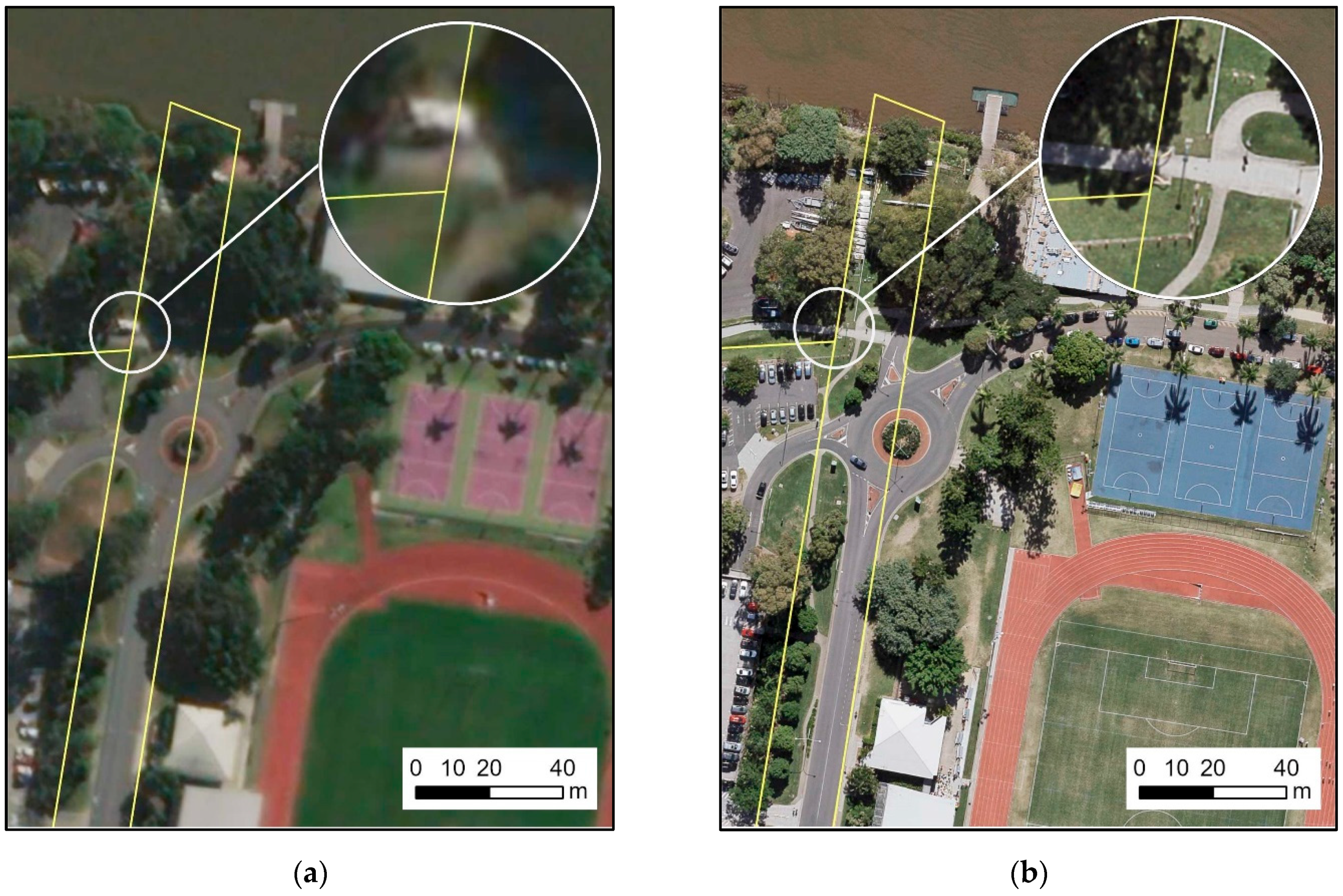
The issue of accuracy has come to the forefront of the spatial sector with improved mapping technology. Figure 1a shows an example of mapped parcels overlayed on a basemap in GIS [13]; with a spatial resolution of ±1 m, there is no obvious alignment issue with other features such as boundary fence lines. Contrast this with Figure 1b that has orthoimagery with a spatial resolution of ±0.1 m; there is a visible mismatch between the mapped parcel boundaries and fence lines. The orthoimagery has a positional accuracy of 0.2 m, so something is misaligned. The same issue of a spatial mismatch would also be apparent on the ground for locating features using low-cost GNSS devices with corrected coordinates via signal augmentation [14], which also have a positional accuracy of approximately 0.2 m. It is the cadastral mapping that is at fault with boundaries out of place by 3–5 m; this is unacceptable by modern standards.

It is possible to zoom into the map in Figure 1b and see places that visibly match fence lines, and other places that do not. This is symptomatic of the varying accuracies for cadastral mapping. It is tempting to simply update the cadastral mapping from higher-resolution orthoimagery, but unfortunately this is also unreliable. It would require good visual coverage of ground evidence of all boundaries, in which is difficult in built-up areas; for instance, there are no fence lines further down the road in the orthoimagery in Figure 1. Cadastral maps should faithfully depict the pattern of parcel boundaries; so ultimately a solution will rely upon better integration of survey plan information and improved mapping.

Improving the accuracy of cadastral mapping is imperative, as it is a foundation layer for national spatial data infrastructures [15]. A strategic approach to achieve this is to systematically improve spatial accuracy levels over time [16,17]. An accuracy level that reconciles boundary coordinates with survey plans is termed survey-aligned. If it achieves a higher accuracy where boundary coordinates have legal status, this is a survey-compliant digital cadastre. The next level is a legal coordinate cadastre, where—in the absence of contradictory evidence—coordinates may be used to re-instate legal boundaries. Countries that have implemented this, such as Austria [18], are small in land mass and have a high density of GNSS control points to support a legal coordinate cadastre. In the interim, a survey-aligned cadastre does support integration of cadastral mapping with other geographical information, but this is not suitable for all cadastral purposes such as resolving adjoining land-owner encroachment disputes. In Australia, survey-aligned cadastral data are published as a digital cadastral database (DCDB), but its accuracy varies significantly. Grant et al. [17] presented a questionnaire to a wide group of land administration stakeholders and found that the ideal positional accuracy for a spatial cadastre is 0.1–0.2 m in urban areas, and 0.3–0.5 m in rural areas.

A supposition of this paper is that a survey-aligned cadastre should align visually with property boundaries shown on a high-resolution orthoimage with a positional accuracy of 0.1–0.2 m in urban areas and 0.3–0.5 m in rural areas. If cadastral mapping had this accuracy, then it would match with visible features for other mapping layers, and would satisfy administrative uses of the data.

This paper explores the following objectives to improve the accuracy of cadastral mapping using a least-squares adjustment that:

• Incorporates higher-accuracy survey control connections and some boundary measurements from source survey plans, and
• Can interpret post-adjustment diagnostics to identify and correct weaknesses in the network.

This paper explores these objectives for updating cadastral mapping using two examples: (i) a test study of approximately 15 hectares for the University of Queensland shown in Figure 1, and (ii) a hypothetical grid for simplified testing. Overall, this paper aims to test if a subset of the underlying data from survey plans is adequate for updating cadastral mapping.

2. Methods

A mapped cadastre may be structurally represented as a network, with parcel corners as nodes and parcel boundaries as edges; it is embedded in space so the corners have coordinates and the edges have directions. Possible values for measured elements may be stored as attributes. In the absence of more precise data, attributed edge lengths and directions are derived by coordinate calculation and include a random error component [19]. Data obtained from dimensions on survey plans have a higher pedigree, and its attributed dimensions are recorded with a much smaller error component. The network structure allows different possibilities to compute the geometry for elements. The error component factors into this and it is desirable to give higher influence to more precise measurements. This is the principle behind network adjustment, namelymore weight is given to accurate data. The attributes for cadastral mapping are treated as an observation network model [20] which includes a functional model to relate geometric elements, and a stochastic model for weighted error propagation. Cadastral maps are spatially generalized to remove details, in comparison to survey networks which include details or a summary for each observed measurement. It is likely that the error component varies for each data element, but is assumed to have an averaged value related to the map scale [21].

Least-squares adjustment finds the best fit to solve the network observation model that minimizes the overall error, e.g., the weighted sum of the errors. Survey networks observe measurements as primary data, and measurement errors are normally distributed. So mathematical rules may be applied for propagating the variances for measures. See Ogundare [20] and Wolf and Ghilani [22] for further details on adjustment of survey networks. The elements of cadastral maps have secondary data where measures are derived indirectly from coordinate calculations, and are assigned an approximate error component. For convenience, it is quantified as a standard deviation or root mean square error, but it is an estimate that varies widely. This is not an issue for the least-squares adjustment procedure itself, as the error component is treated as a weight in adjustment. It is more of an issue for the post-adjustment analysis which tests the overall accuracy based on t-scores, z-scores and chi-squared statistics. As an alternative, this paper explores post-adjustment effects of coordinate shifts at corners and changes to derived distance measurements for boundaries. This is consistent with interpreting adjustment as a rubber-sheeting process, where coordinate shifts are analogous to stress acting on the network, and strain as the corrected distance for network edges. Stress–strain relationships are applied in structural mechanics to determine stress and displacement of a structure under load. It is intuitively interpreted as an external stressor acting on connected finite elements, resulting in distributed deformation [23]. Finite elements methods have been used to evaluate the internal adjustment reliability of survey networks from induced deformations by errors in measurements [24,25]. The aim is to relate the local coordinate displacement of points to differential deformation of the connected geometry. Mathematically, this may be determined by possible errors in network line measurements (strains) and network configuration. Reliability means adjusting a network results in small point displacements; on the other hand, large point displacements indicate gross measurement errors or a weak network configuration. Other approaches directly applicable to parcel geometry are based on rubber-sheeting concepts for triangulating and adjusting parcels [26].

The software used in this paper is the Parcel Fabric Extension in ArcGIS Pro [13]; this represents spatial features for: (i) property parcels and line boundaries with direction and distance dimension attributes, and (ii) control points and their survey corner connections. The GIS environment provides many spatial data management functions, and specialized tools to edit the coordinate geometry of boundaries and adjust boundaries to control points or more accurate boundary line measurements. The adjustment fits the weaker geometry of the parcel fabric to survey control; typically, it weights the angular measures at boundary corners and boundary distances to maintain the shape of parcels.

The next sections explore adjustment of cadastral mapping for a small case study area shown in Figure 1, and a hypothetical grid where it is easier to explore the effects of adjustment.

2.1. Least-Squares Adjustment of Cadastral Mapping Using a Small Area Example

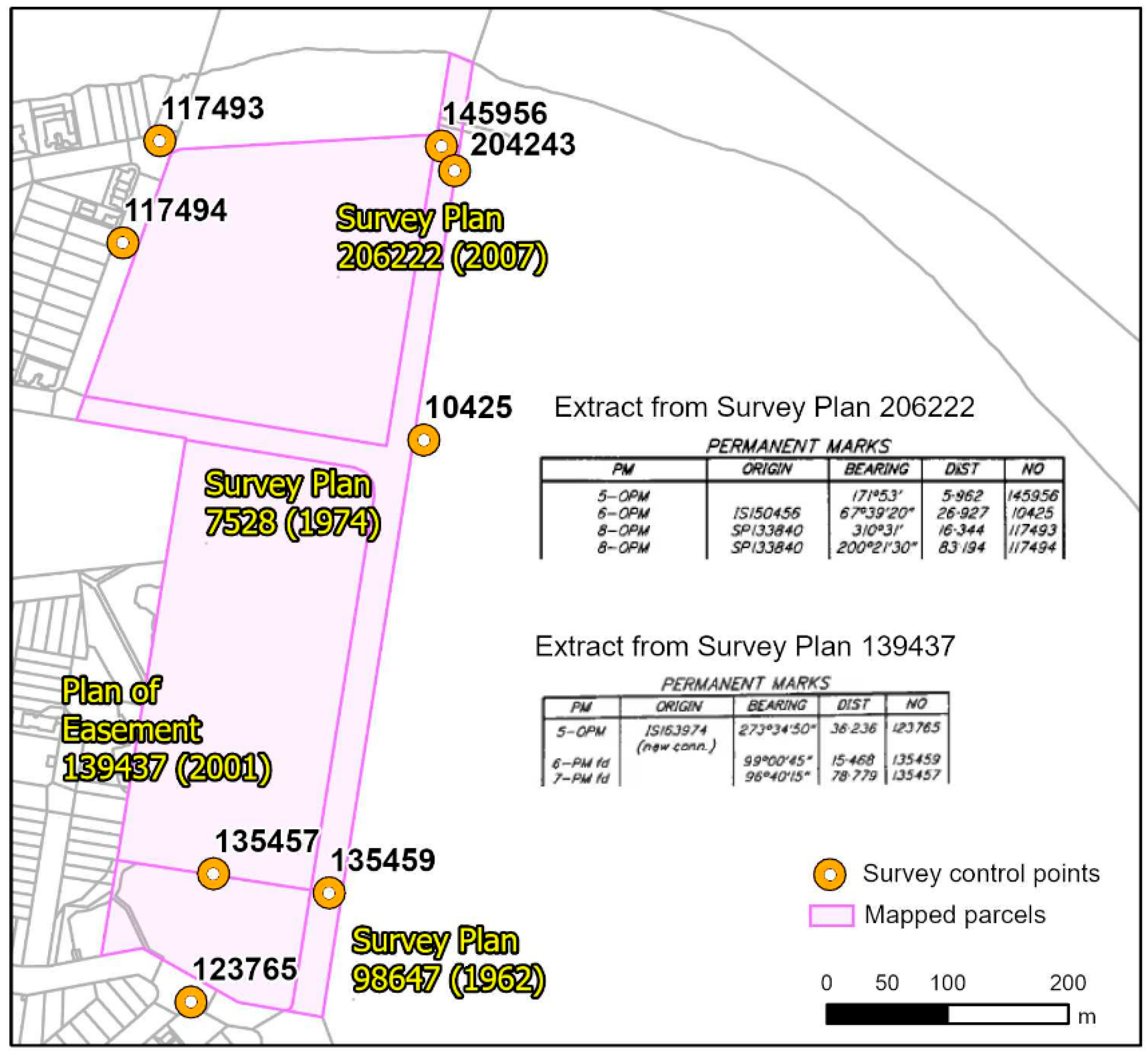
The purpose of this example is to demonstrate updating cadastral mapping with control points. Cadastral surveys record connections (distance and direction) from permanent survey marks to parcel corners; see Figure 2. It is common practice to observe a GNSS coordinate to permanent marks for current cadastral surveys, or to revisit the site and observe it for earlier surveys. The survey control marks provide a ready source to update cadastral mapping and improve its accuracy.

A least-squares adjustment procedure may be applied to adjust the lower accuracy derived measurements (boundary lengths and directions) from cadastral mapping to fit with the higher-accuracy survey control that connects to corners. Earlier approaches to integrate new spatial data into cadastral maps were based on geometrical transformations; but these methods did not constrain new parcels to fit with adjoining parcels. Least-squares adjustment was found to be a promising alternative [27]. It was developed to adjust measurements in survey networks [22], but is applicable to cadastral mapping when boundaries are represented with coordinate geometry attribution in GIS. Least-squares adjustment has proven to be a versatile addition to GIS for incorporating area constraints [28] and boundary line collinearities [29].

We investigate updating the cadastral mapping for a 15 hectare urban area near the university. The data were extracted from a statewide digital cadastral database (DCDB) with a stated map publication scale of 1:2500 and map accuracy of ±1.5 m [30]. Despite being a small area of just 4 parcels and 40 boundary lines, it does exemplify cadastral mapping problems. The two main problems are: (i) parcel corners with positional errors greater than ±1.5 m (as discussed in Introduction), and (ii) a poor degree of conformity with original survey dimensions. Figure 2 shows the extracted parcels and locations of permanent control marks in their vicinity; all control marks have corner connections. ArcGIS Parcel Fabric [13] was used to represent parcels and their boundaries; the workflow process is: (i) build the parcel and boundary features, (ii) compute coordinate geometry direction and distance attributes for boundary lines, (iii) assign accuracies as further attributes (±1 m for distances, and ±1/10 degree for directions based on DCDB metadata), (iv) add survey control points (constrained to fixed map coordinates), (v) add connections from parcel corners to the survey control, and (vi) analyze the network with a weighted least-squares adjustment. The adjustment computation is performed by the DynAdjust package [31] integrated into ArcGIS, which is capable of analyzing large geodetic, survey and cadastral networks.

The Parcel Fabric Extension in ArcGIS Pro [13] is used for the adjustment. It provides tools to prepare data for adjustment, which includes setting accuracies on control points, connections and boundary lines. Datum control points were constrained to be fixed, and coordinate-derived line distances and directions are given low accuracies, ±1 m and ±1/10 degree, respectively. In a least-squares adjustment, the accuracies act like weights, where low-accuracy measurements have a lower influence on fixing the adjusted geometry. Further details on the adjustment process may be found in ArcGIS documentation for Parcel Fabric [13].

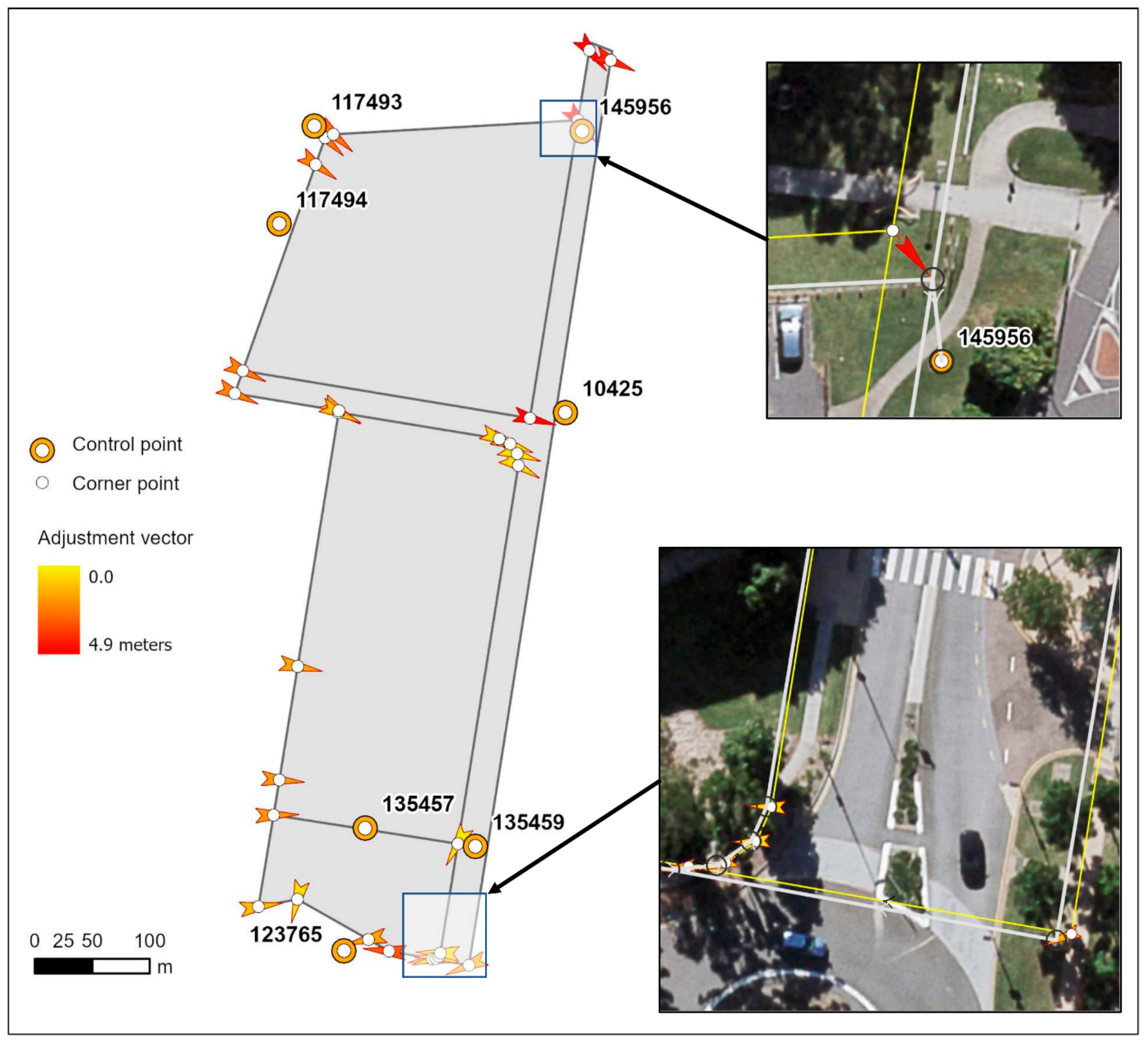
Figure 3 shows the results of a least-squares adjustment that reconciles the higher-accuracy corner connections to permanent survey marks with the lower-accuracy geometry of the cadastral mapping. Least-squares adjustment will retain the geometry form of parcels, but constrained to fit with the control. Looking at the results overlayed with orthoimagery at the northern end near the river, the adjusted boundaries now align well with fences and other features. On average, coordinate displacements to corners (shown as adjustment vectors in Figure 3) are 2.5 m and an adjusted standard deviation of 0.4 m. This indicates remaining errors in the cadastral mapping. In locations that do not have visible evidence of boundary features, it is difficult to identify what is at fault; this occurs at the southern end of the road due to recent development of a major transit center for the university.

In summary, adjustment to the survey control does improve the mapping, but it also highlights areas with large discrepancies. The difficulty is distinguishing what are significant discrepancies in calculated boundary measurements from the cadastral mapping. The next section attempts to break this problem down further by exploring relationships between corners (coordinate displacements) and the boundary lines (corrected length dimensions). The aim is to develop a post-adjustment diagnostic to isolate large errors in the cadastral mapping; as it is possible to fix this where needed with additional control or better survey plan measurements. The next section analyses a simpler network to reveal how error is propagated in this type of adjustment.

2.2. Cases for Least-Squares Adjustment of a Uniform Measurement Grid

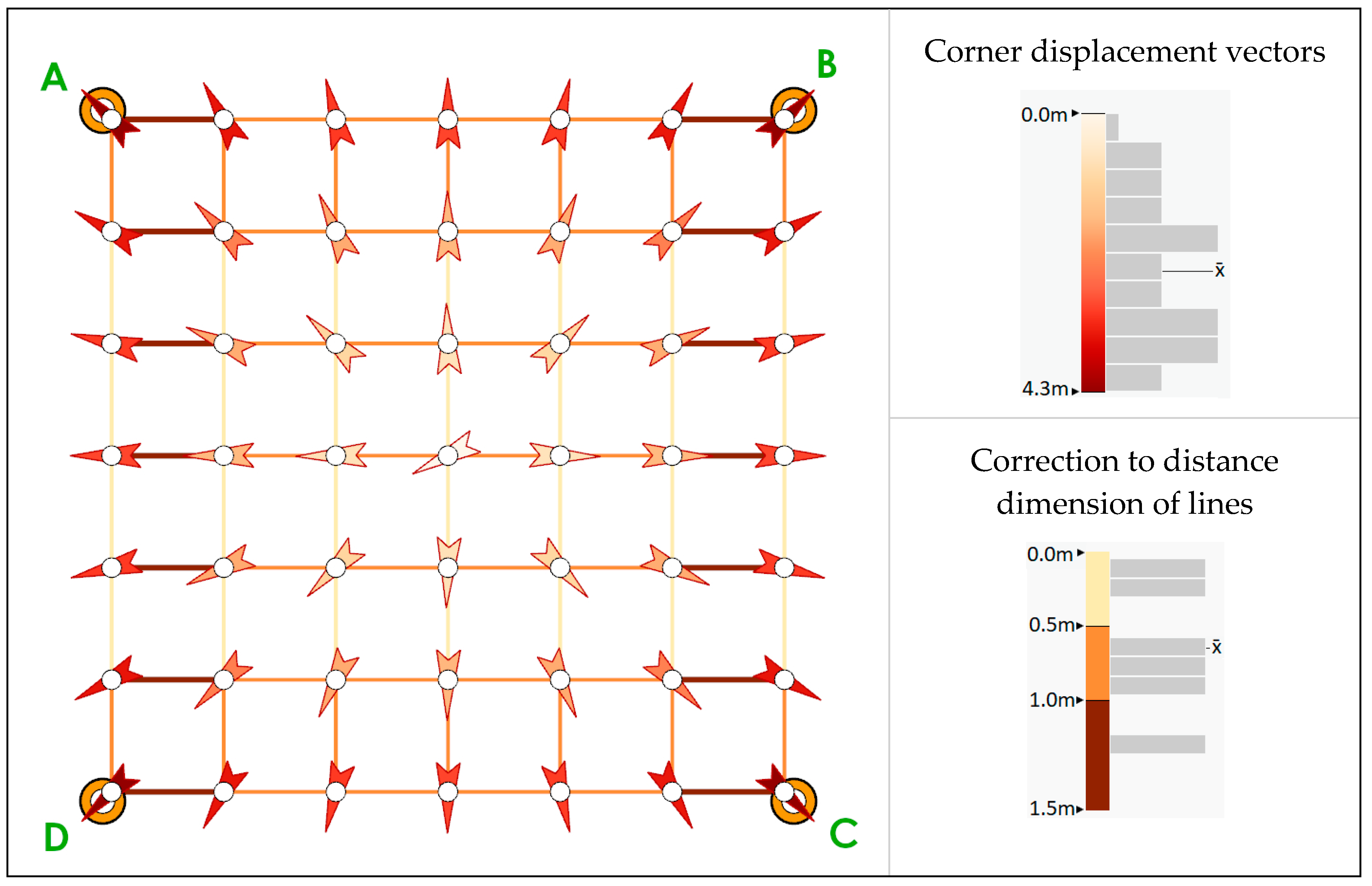
This section explores characteristics for least-squares adjustment given different network configurations, and ways to improve the adjustment results from control or boundary measurements. A hypothetical grid composed of 6 by 6 uniform cells (parcels) of 1 hectare is assumed to have been contracted in scale to fit with inexact mapping. To keep it simple for explanation, each edge is initially given a computed length by its end-point coordinates which is in error by 1 m, and assigned a standard deviation of ±1.0 m. It is further assumed to have connections to exact survey control at the four grid corners, these are labelled A, B, C, D in Figure 4.

Using the example data, three adjustment scenarios are explored:

• Case 1—Using well-distributed connections to survey control at the corners;
• Case 2—Using connections to survey control at three corners, but one corner has no connection;
• Case 3—As above, but some sides have precise distance and direction measurements.

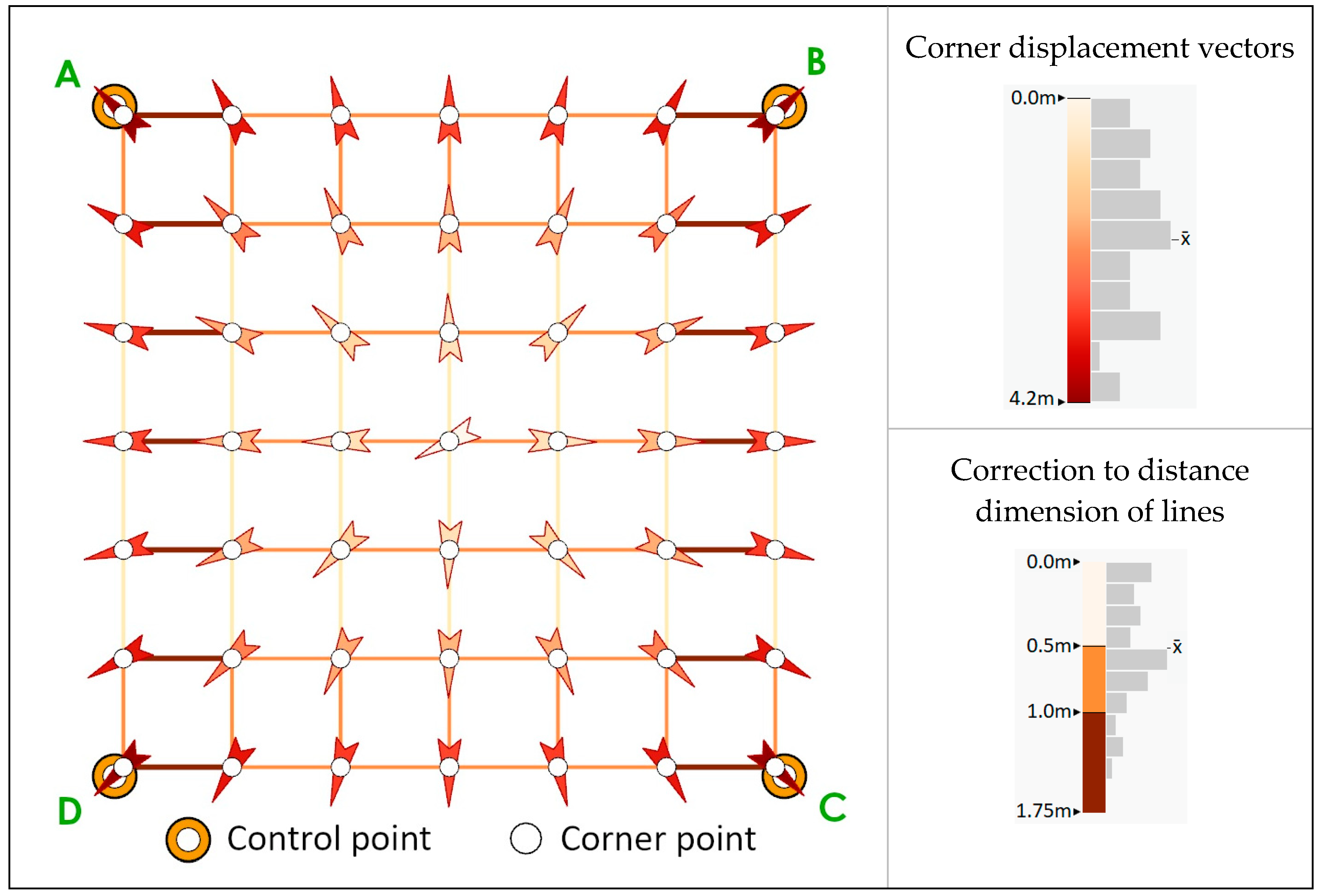
Case 1 is shown in Figure 4. The grid is to be adjusted to fit to the four constrained control points A, B, C and D. The results of applying a least-squares adjustment will correct all grid corners to the control and scale the distances of all edges. Post-adjustment corner displacements, shown in Figure 4 as arrows, have a uniform pattern of displacement outwards to fit to the four control corners. Changes to edge distances should be approximately 1 m, but this is not exactly as expected due to the iterative adjustment process.

The adjustment is analogous to stretching the grid in a rubber-sheeting sense, where moving points outward indicate stress, and corrections to edge distances indicate strain. Edges have a post-adjusted standard deviation for distance of ±0.3 m (an improvement from ±1.0).

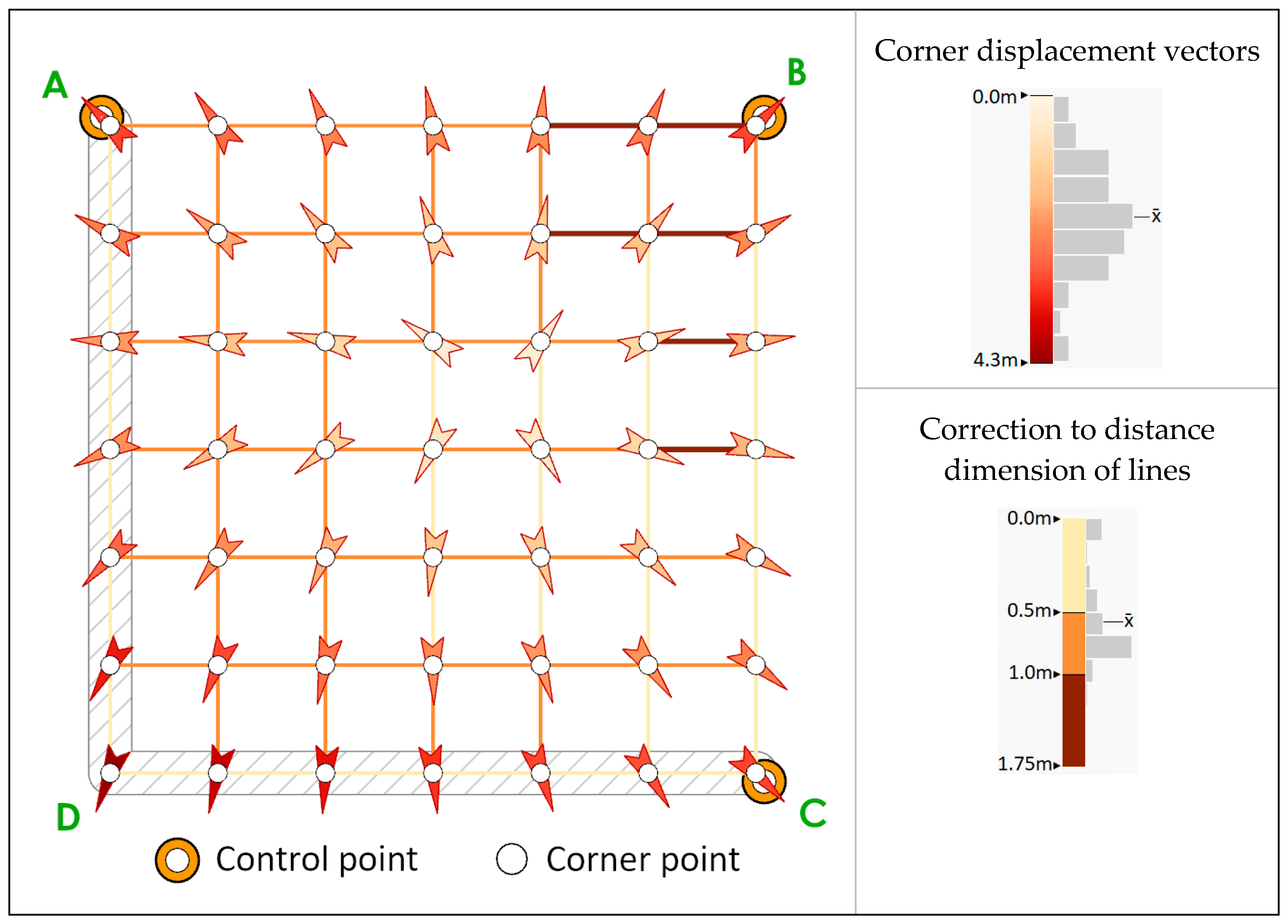
Case 2 is shown in Figure 5. This is different from the previous case in that the control point at D is removed and not used for adjustment. The results of applying a least-squares adjustment is now not uniformly scaled; the grid is more deformed in the bottom-left corner, where there is no control point connection. The grid is adjusted to fit to control points at A, B and C; this is analogous to stretching to fit these corner locations. The adjustment is propagated along network edges, but the lack of control near D means it is less stiff and will deform more. The edges near corners labelled A, B, C have a post-adjusted standard deviation for distance of ±0.4 (an improvement from ±1 m) and the corner labelled D has a post-adjusted standard deviation for distance of ±0.5.

Case 3 is shown in Figure 6. This differs from the previous case by changing the edge lengths along the left and bottom sides to their exact distance and with a higher accuracy, e.g., a lower standard deviation of ±0.1 m. In terms of the rubber-sheeting analogy, some sides have extra stiffness to resist distortion. The edges along the sides D–A and D–C act as a right-angled brace imposed on the grid at corner D, and the remaining grid is stretched to fit with control at points A, B, C. This highlights a characteristic of least-squares adjustment where inexact (or unknown) values are improved (or determined) indirectly by the constraints on other quantities that are functionally related by the network geometry [22].

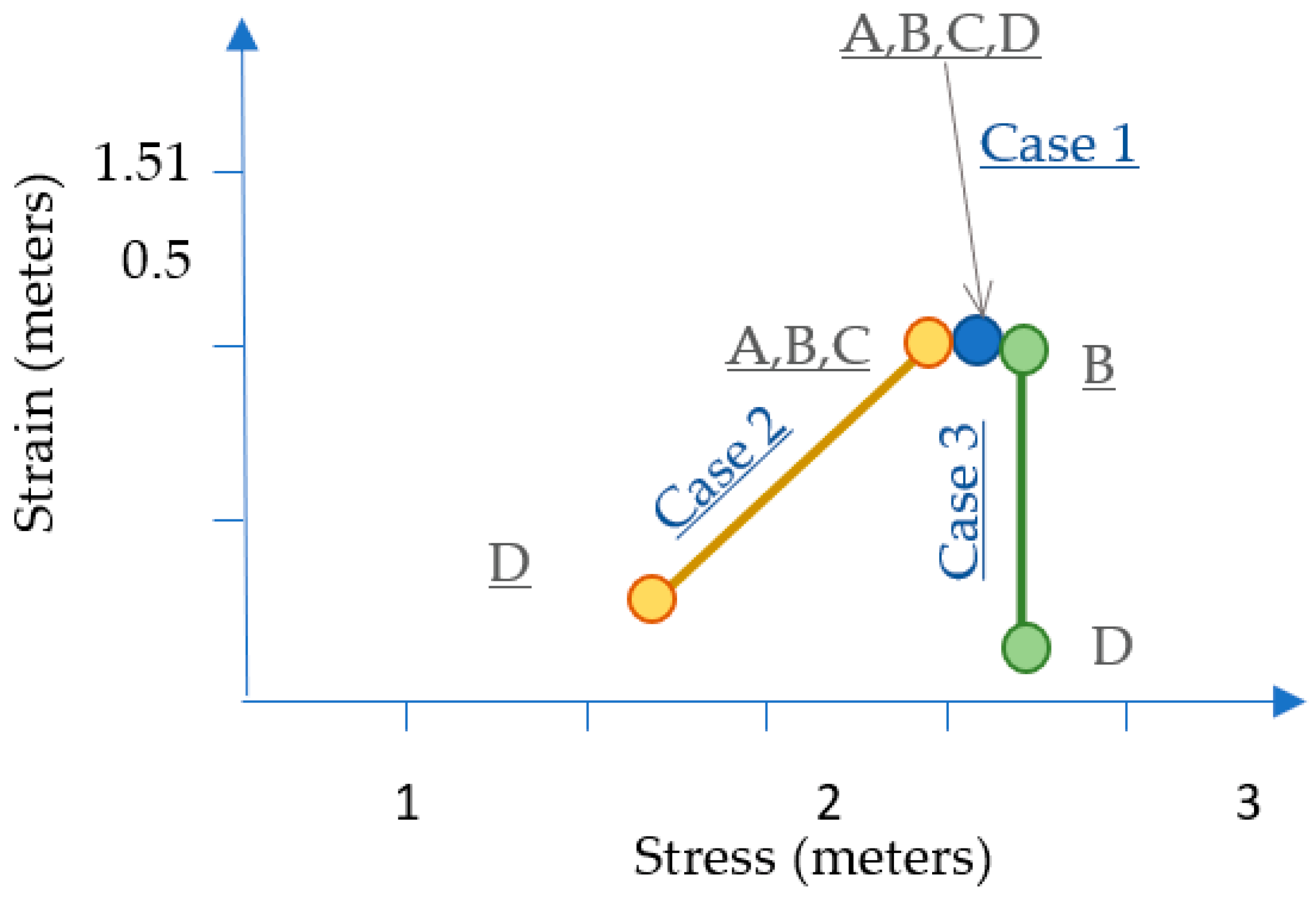
Figure 7 summarizes the three cases in terms of stress–strain relationships for points and lines just at corner locations. Case 1 has evenly distributed survey control so adjustment causes uniformly scaled position displacements (stresses) and edge dimensions corrections (strained) at corner locations labelled A, B, C, D. Case 2 has unevenly distributed survey control, and the corner labelled D is adjusted less, resulting in the grid being warped. Case 3 similarly has uneven survey control but is braced with correct measurements along sides A–D–C, so the edges associated with these sides are stiffer and are moved into place as opposed to being distorted.

The stress–strain relationship provides a means to interpret the a priori and post-adjustment changes in the grid. It also gives clues to reveal weaknesses or outlier dimensions in a network. The best approach is to perform an analysis in two phases: (i) adjust the network with evenly distributed survey control across the study area, and (ii) investigate parts of the network with anomalies for stresses (uneven localized displacements) or strains (in distance and direction dimensions) relative to other parts of the network. The first phase is to rule out lack of control in adjustment so any anomalies may be attributed to other weaknesses, e.g., the variable error component in boundary dimensions. If coordinate control is not available from official sources, then additional GNSS control may be captured for corner connections or cadastral corner locations extracted from orthoimagery [32,33].

In the next section, we explore a more complex network for the university case study that has an unknown variable error component for edges.

3. Results

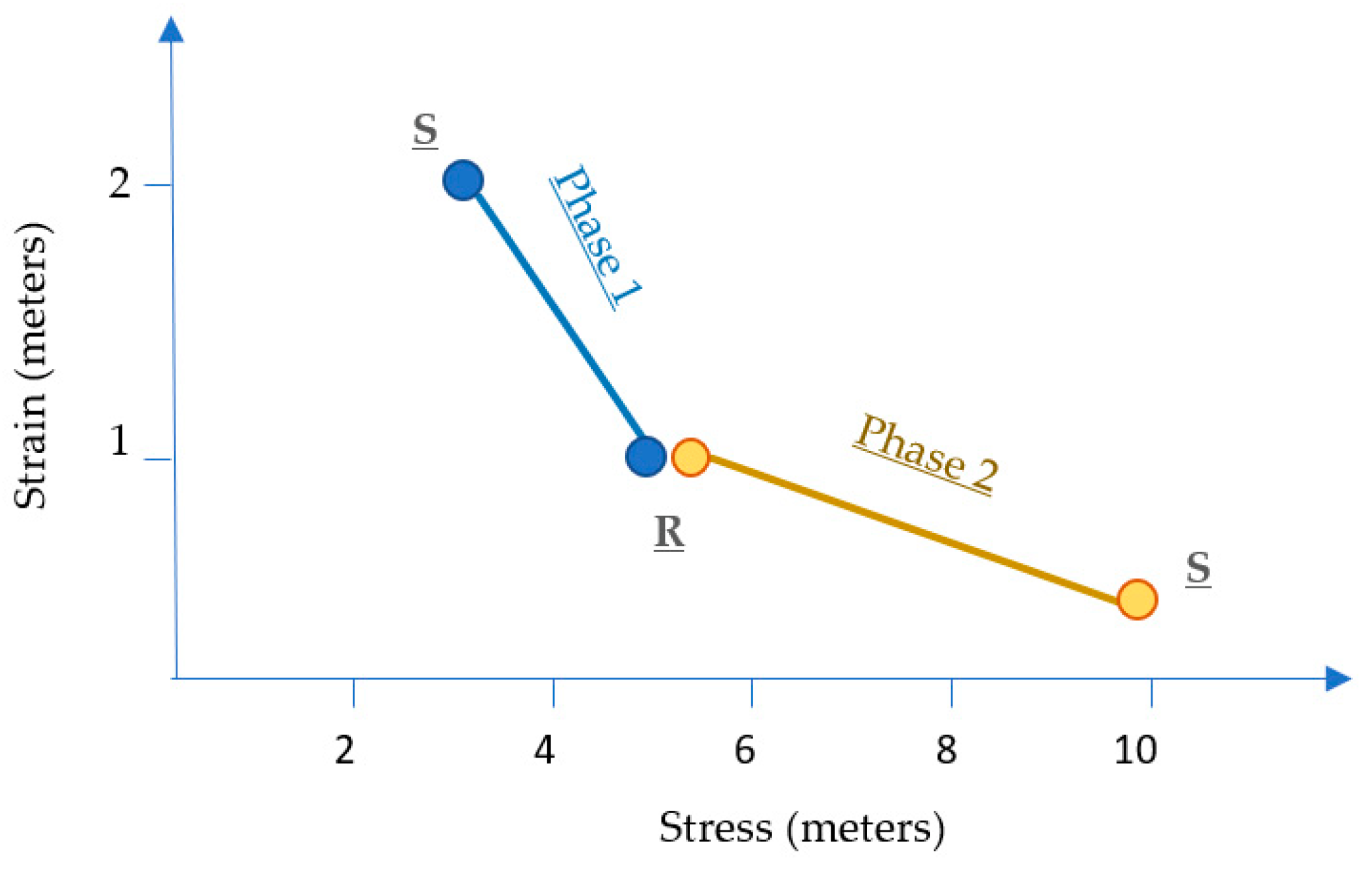
We re-visit the campus example from the introduction with the intent to better understand why large coordinate displacements occur at the southern end of the site when adjusting the cadastral mapping (phase 1). Figure 8 shows the stress–strain chart for post-adjustment of the cadastral mapping. Phase 1 employed a least-square adjustment with available control distributed across the study area. Most corners required coordinate displacements to fit with survey control, the largest being near the river (labelled R), but they had a regular easterly pattern for most corner points and boundary distance corrections of approximately 1 m. The anomaly was at the southern end of the road (labelled S), where there was localized variation in corner displacements and larger boundary distance corrections.

A review of source survey plans revealed a complex series of cadastral surveys along the road over the past 60 years; it appears as if the width for the road was misinterpreted in the cadastral mapping. To resolve this anomaly, survey measurements were taken from original plans along the road and the adjustment re-run (phase 2) with these higher-accuracy measurements. This made the road structurally stiff, so more elastic edges connected to the road are strained to fit to control. This dramatically changed the displacement of points at the southern end of the road (label S), which indicates a large dimensional error in the mapped data for one or more edges. Further investigation of survey plans confirmed a 10 m blunder for the dimension of the road width and related corner positions. Using higher-accuracy boundary measurements along the road resulted in smaller corrections (label S) in Figure 8, indicating less strain. Similar to the grid example, the corrected boundaries were moved into place. Additionally, the weighted (post-adjusted) standard deviation on average was ±0.25 m (as compared to the a priori standard deviation on edge lengths of ±1 m). While there are no fence lines in the locality of the southern end of the road, survey plans did show ties to buildings visible in the orthoimage and this agreed with the adjusted cadastral mapping to confirm a better overall match.

For comparison, all survey plans dimensions were back-captured to exactly test mapping errors. Traverse closure for all parcels was less than ±0.05 m, so measurements are reliable. The average difference between survey plan measurements and cadastral mapping edge lengths is ±4.5 m (root mean square deviation); and after fixing blunders for Phase 2, this reduced to ±2 m. Figure 9 charts the differences without corrections, and the blunder measurements for road widths are apparent as the outer values in the chart.

4. Discussion

This paper has explored the problem of improving the accuracy of cadastral mapping with an adjustment procedure that combines aspects of mapping geometry, more accurate coordinate georeferencing with source survey control and survey plan measurements.

A computational method for adjusting the geometry is used, namely least-squares adjustment. It is conventionally used to adjust primary survey observations with known accuracy. This contrasts to adjusting cadastral mapping, which has inaccurate boundary measurements and unknown variable error components. Nonetheless, least-squares adjustment is an appropriate tool as it makes few assumptions about the nature of errors and provides the means for post-adjustment diagnostics to analyze errors.

We explore two example datasets with the aim to find a way to understand and handle inaccuracies in adjusting cadastral mapping for errors related to: (i) coordinate positioning, and (ii) variable errors in geometry elements, i.e., the lengths and angles.

The two error types interact, making it difficult to give reliable results. A tractable solution is to initially fix the positioning with survey control, and analyze residuals for the adjusted measurements to detect weak geometry or blunders. This can be partly fixed by adding higher-quality measurements available from cadastral survey plans to improve the overall geometry.

The first example uses a grid with inherent mapping inaccuracy, but its regular geometry provides insights on the effect of adjustment. Case 1 shows an adjustment constrained to fit with survey control that scales the grid and improves its accuracy. Interpreted in terms of rubber sheeting, the grid is stretched (stressed) to the survey control and derived measurement dimensions strained to adjust accordingly. Case 2 shows the effect of poorly distributed survey control causing uneven warping of the grid and adjustment differences in the uncontrolled parts of grid. This may be corrected by: (i) adding extra control (as in case 1), or (ii) adding higher-quality measurements in parts of the grid where anomalies are detected (case 3). This last option is satisfied in a real-world study by extracting measurements from the original survey plans. It is anticipated that extracting survey plan dimensions along major roads would strengthen the cadastral geometry, and provide useful information for relating other land information assets.

The second example used a portion of cadastral mapping in the vicinity of the campus. Survey control was available from permanent survey marks with GNSS coordinates and connections to cadastral corners. Using a staged approach, an initial adjustment of the cadastral mapping to the survey control showed an improved fit and better alignment with fence lines visible in high-resolution orthoimagery but it also highlighted anomalies at the southern end of the study area. The anomaly was apparent visually as random directions for corner displacements, and localized differences in the adjusted boundary dimensions. To resolve this anomaly, original survey measurements with a higher accuracy were extracted from survey plans and incorporated in the cadastral mapping. A second adjustment fixed an incorrect measurement for the width of the road; and on visual inspection, the mapped boundaries aligned well with orthoimagery with a post-adjustment accuracy of ±0.25 m on boundary lengths. The effort to obtain the extra survey data from original survey plans was minimal, e.g., corner connections to survey control and four survey dimensions along the road. It is substantially more effort to back-capture all the survey plan measurements [3] for a survey-compliant cadastre.

5. Conclusions

This study suggests a cost-effective and tractable way to improve the accuracy of cadastral mapping and to remedy blunders detected in mapping. It provides confidence to use cadastral mapping for a wide range of land administration applications, e.g., mapping related to land ownership, tenure, roads and other built infrastructure. The approach is most suitable in jurisdictions that historically use a cadastral map as an index to register the relationship (rights) between people and land, and as a register of fixed boundaries [7]. It is desirable to make cadastral maps accurate to use as a GIS layer for land tenure, but this is challenging to spatially resolve the geometric dimensions from survey plans and positional accuracy of modern mapping. It is possible to perform area-wide updates using a procedure such as least-squares adjustment from GNSS-accurate control points linked to surveyed parcel corners; but to achieve a higher level of accuracy, all measurements from survey plans must be reconciled, a far more complex exercise.

Another by-product of this study is interpreting the post-adjustment results with stress–strain mapping and charts. It is problematic to equate the error component in cadastral mapping measurements statistically, and such statistics can be difficult to understand within a distributed network of measurements. For GIS mapping professionals—unfamiliar with computational principles for least-squares adjustment—it is desirable to have simple graphical diagnostics to interpret results for corner displacements and corrections to boundary edges. A future aim is to explore this paradigm for interpreting adjustment results in terms of stress–strain relationships with more extensive and complex cadastral mapping case studies.