
Probability-Based Strategy for a Football Multi-Agent Autonomous Robot System
 , ,
, ,  , ,
, ,  and
and
Abstract
:1. Introduction
2. Related Work
2.1. Most Common Used Architecture
2.1.1. Skills
2.1.2. Tactics
2.1.3. Plays
2.1.4. Playbook
2.2. Machine Learning Approaches
2.3. Different Play Transition Methods
2.4. Alternatives to STP
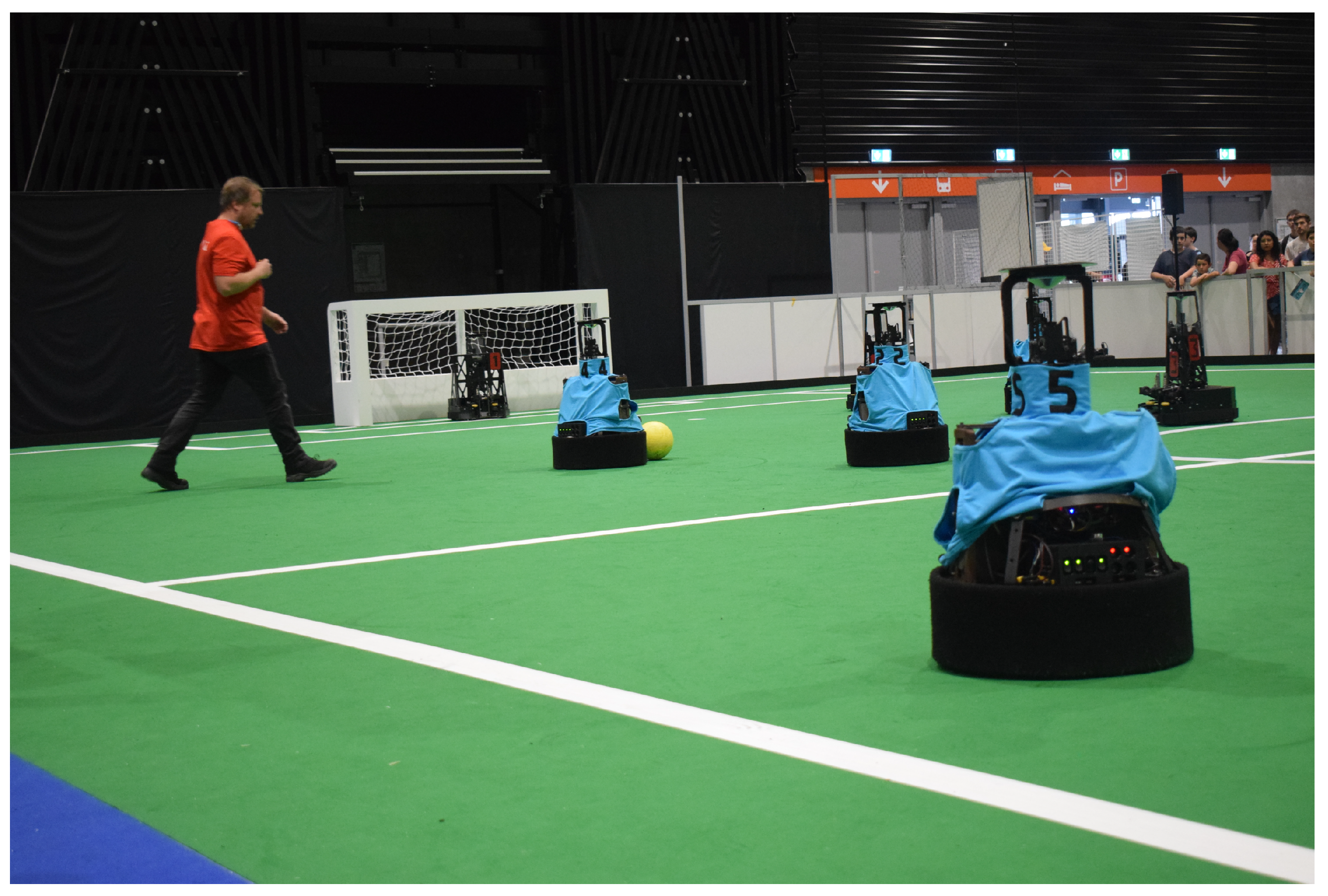
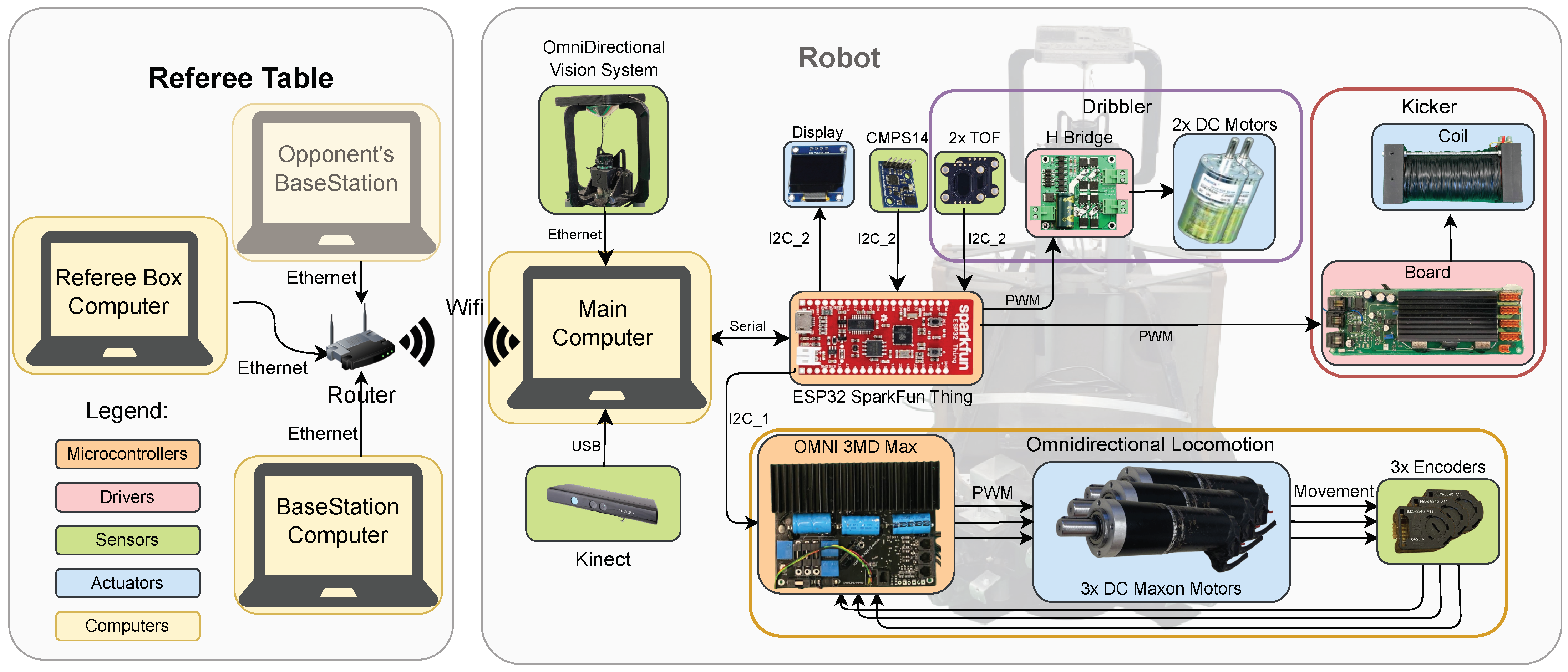
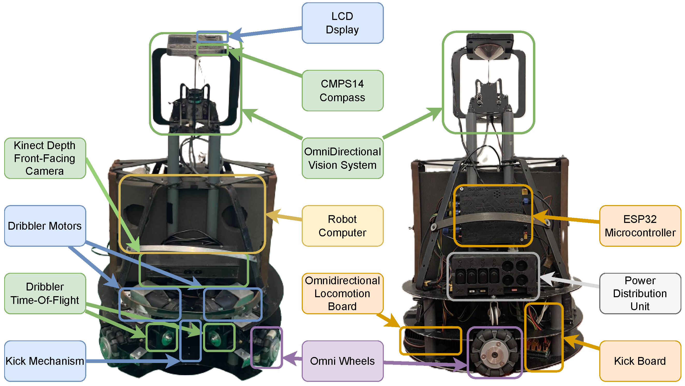
3. Robots Hardware
4. LAR@MSL Skills
4.1. Stop
4.2. Move
4.3. Attack
4.4. Kick
4.5. Receive
4.6. Cover
4.7. Defend
4.8. Control
5. Strategy
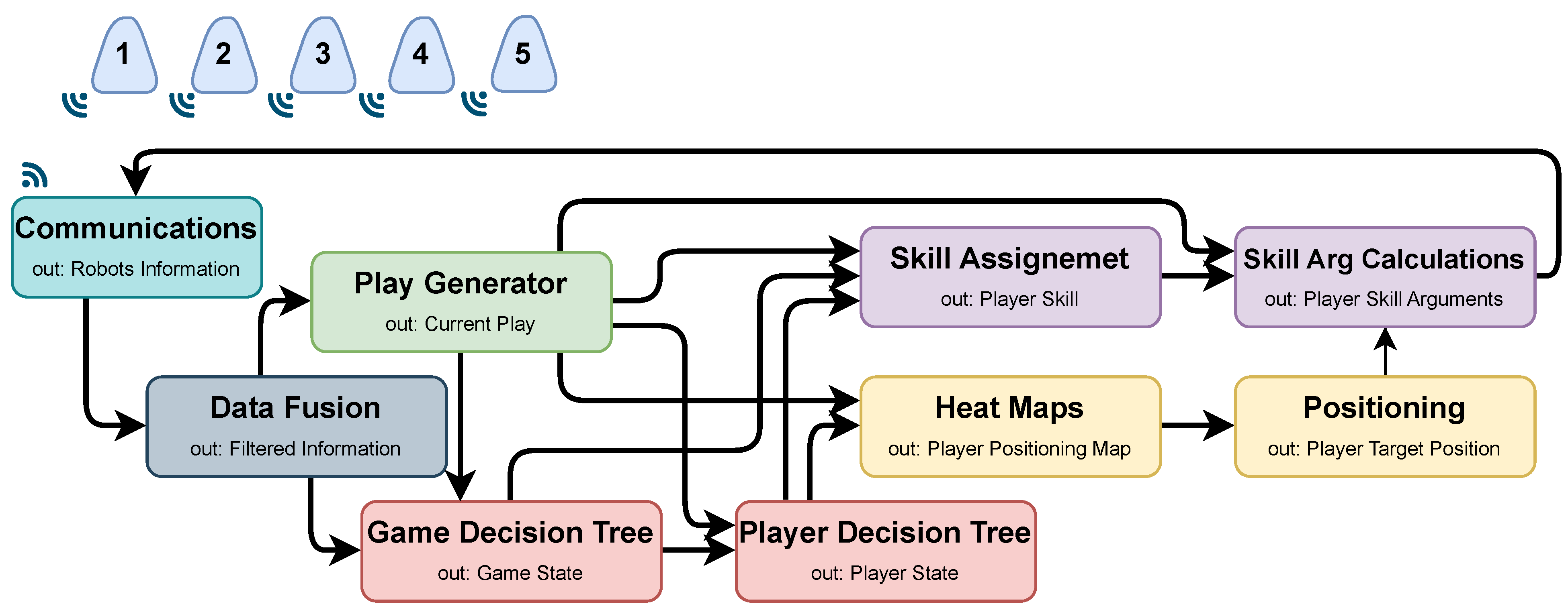
5.1. Architecture
5.2. Play Generator
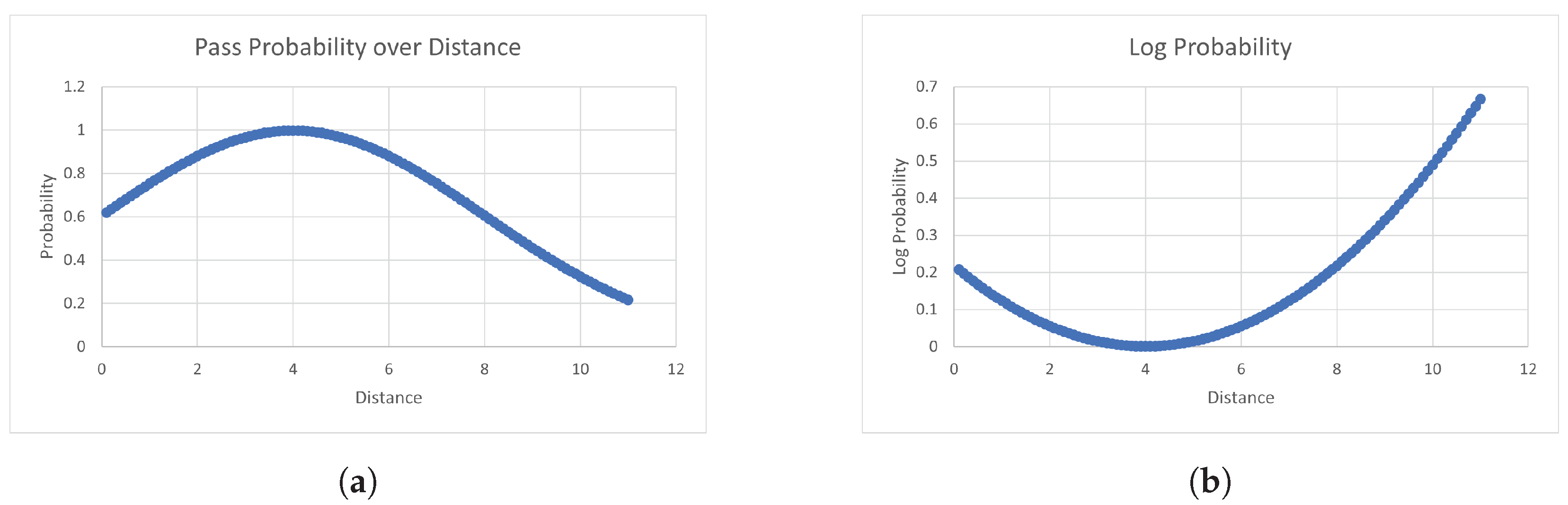
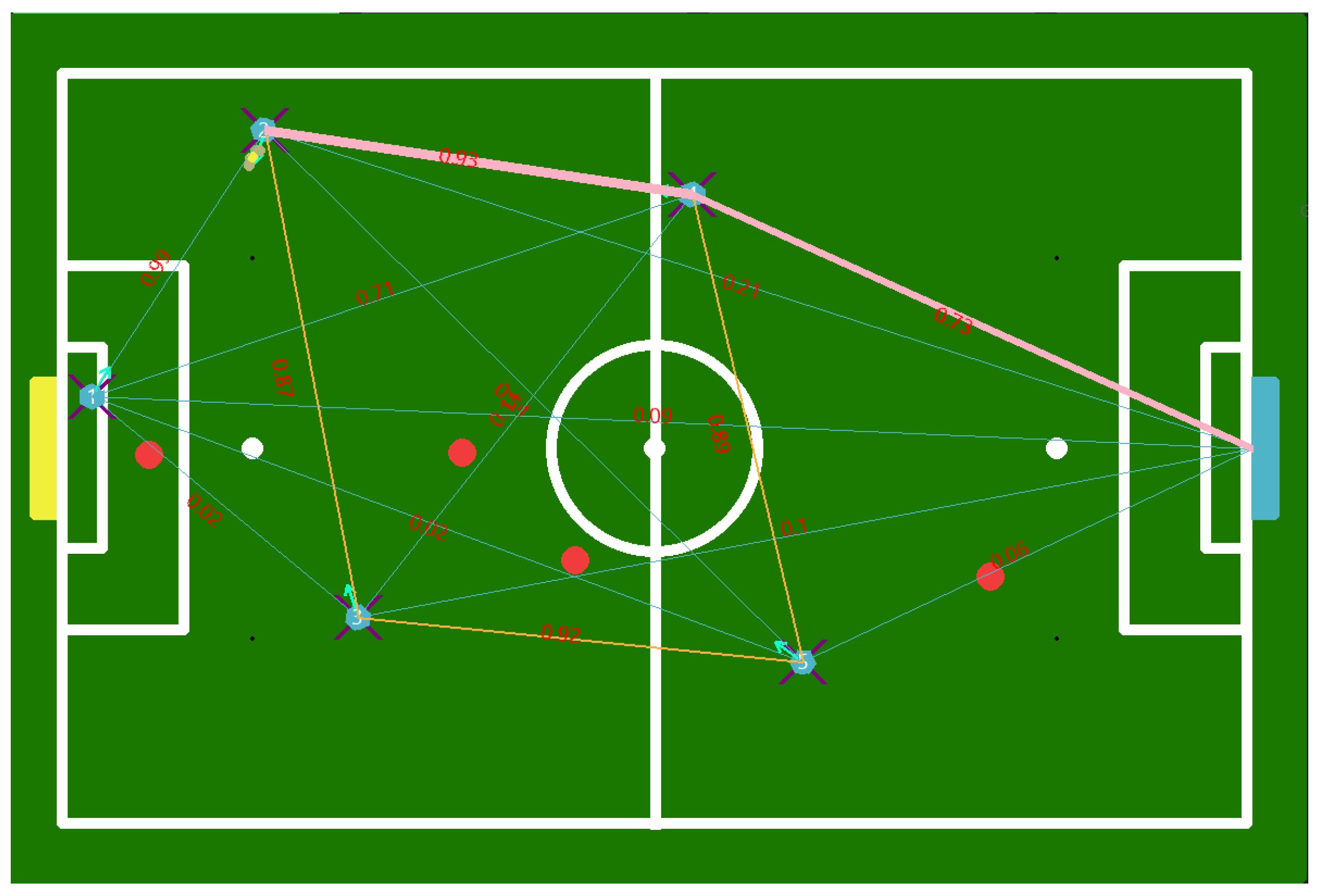
5.3. Probabilities
5.4. Log Probability
5.5. Graph Generation and Path Finder
6. Decision Trees
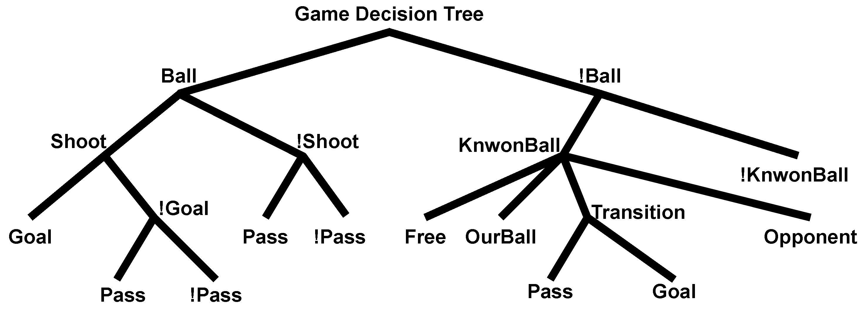
6.1. Game Decision Tree
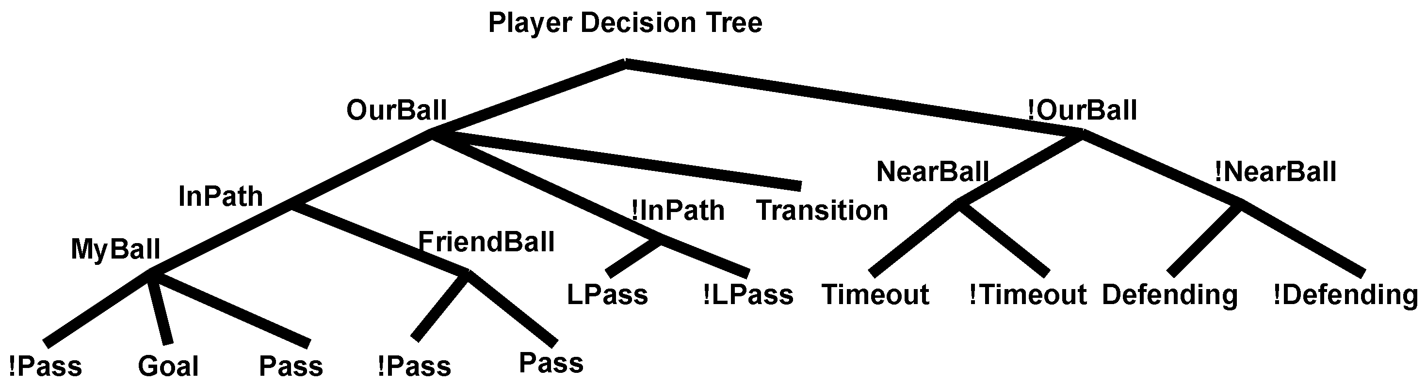
6.2. Player Decision Tree
7. Heat Maps and Positioning
7.1. Information Used for Positioning
7.2. Zones
7.3. Maps Generated
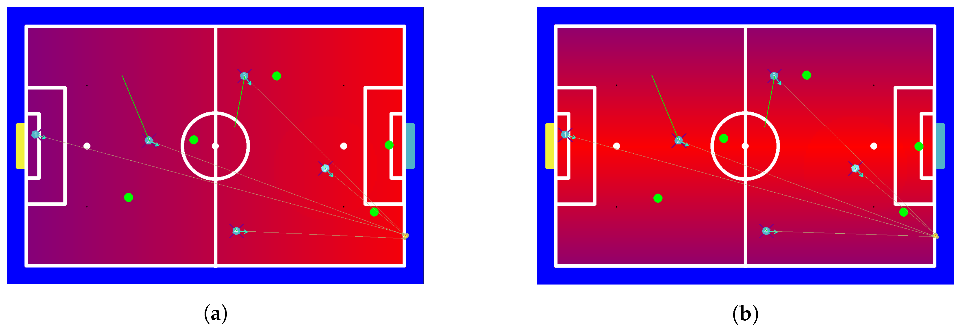
7.3.1. Middle Field and Center Field
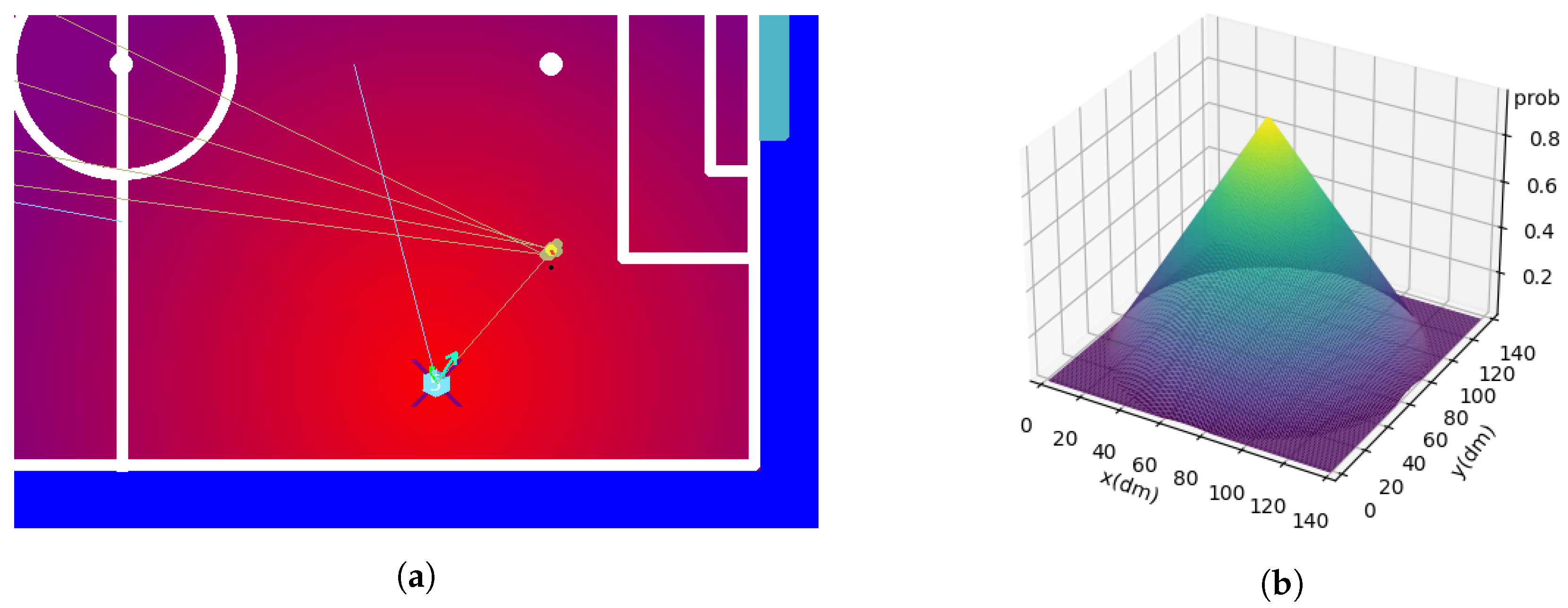
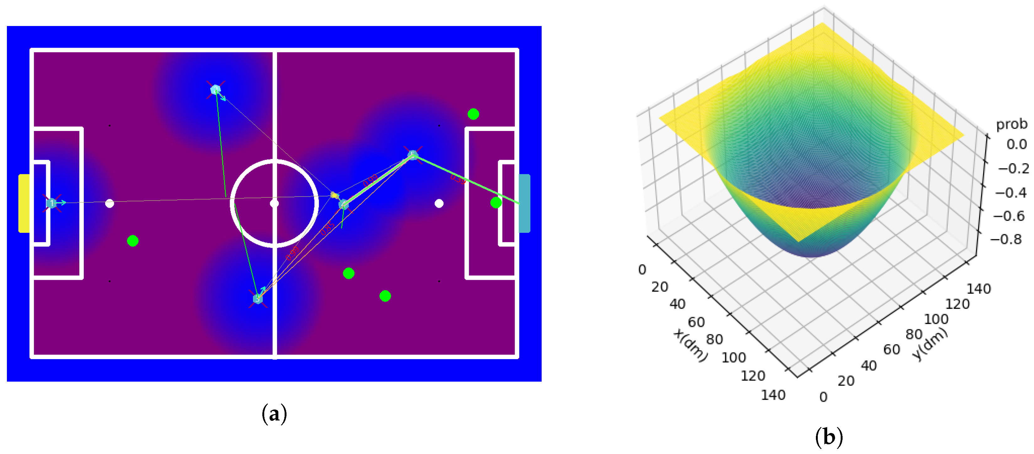
7.3.2. Ideal Pass Distance
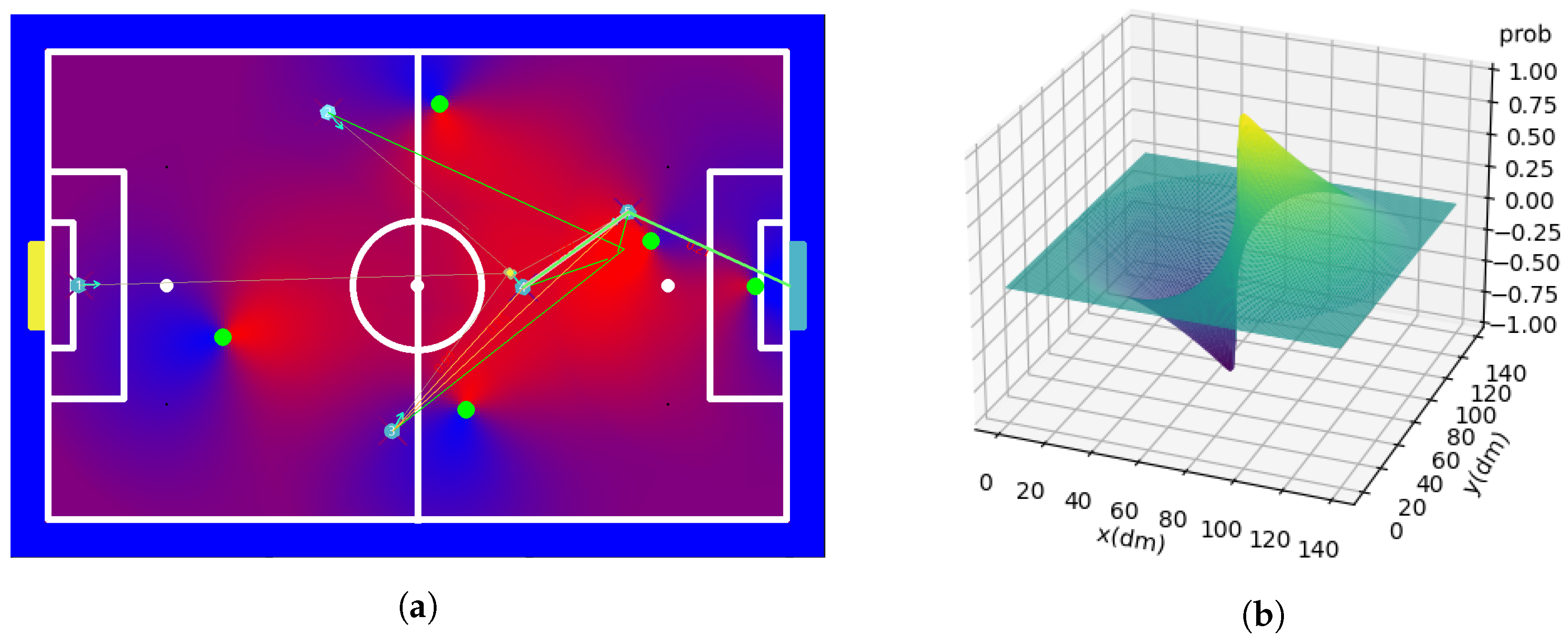
7.3.3. Ideal Goal Distance
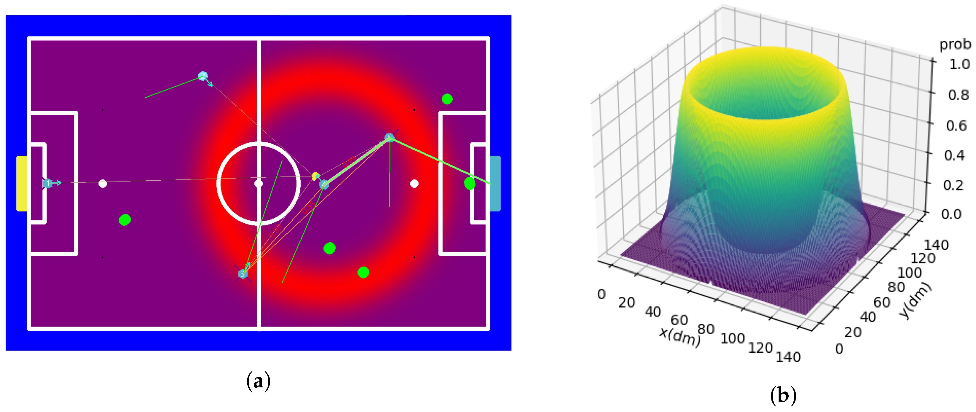
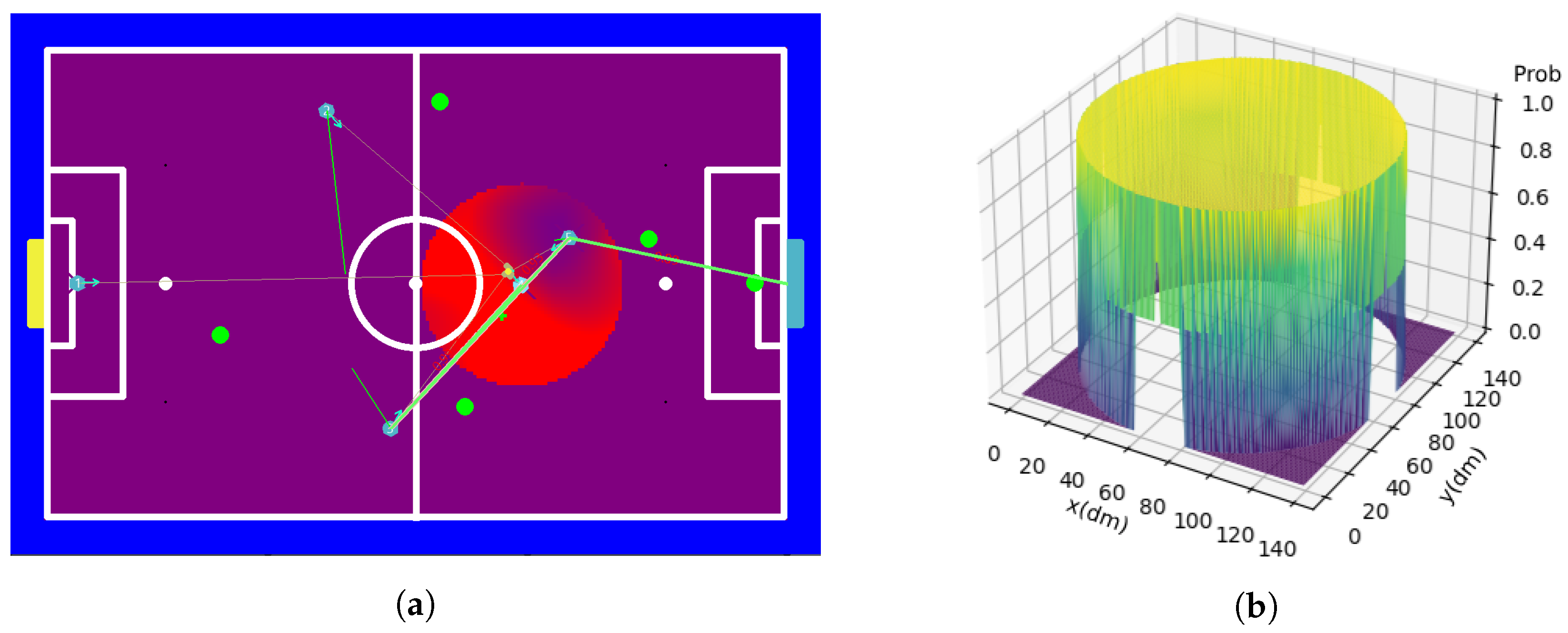
7.3.4. Opponents Circle
7.3.5. Teammates
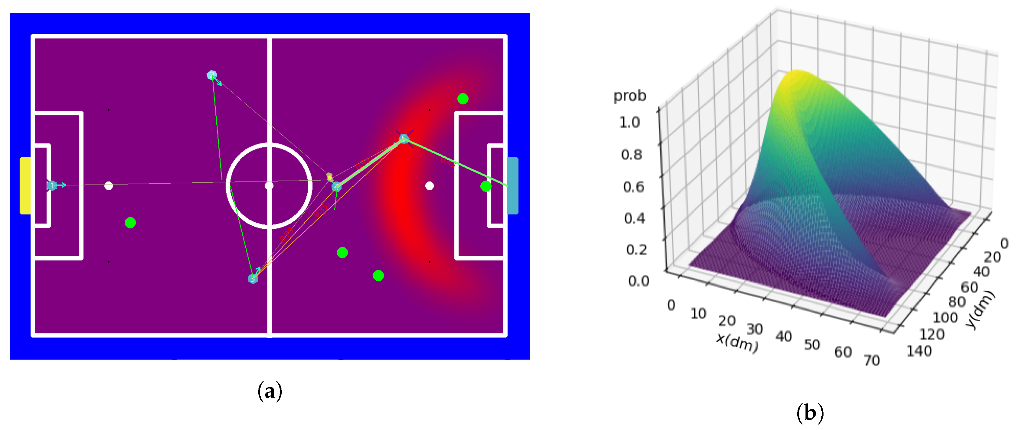
7.3.6. Opponents Cone
7.3.7. Three-Meter Radius with the Ball
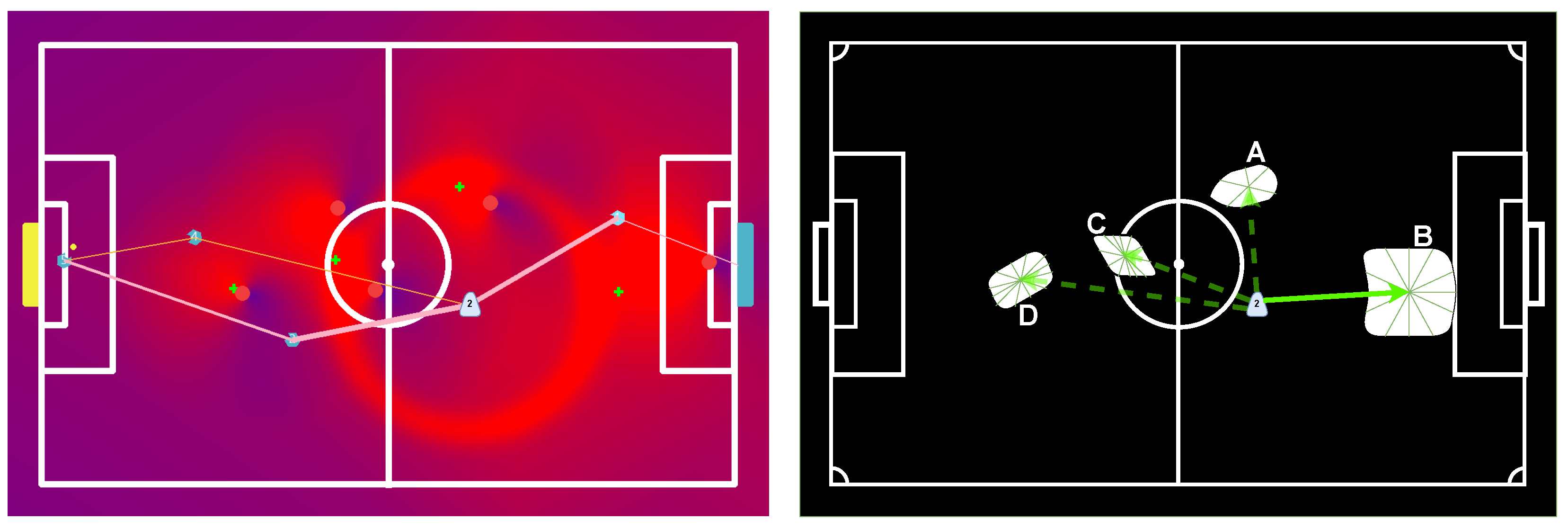
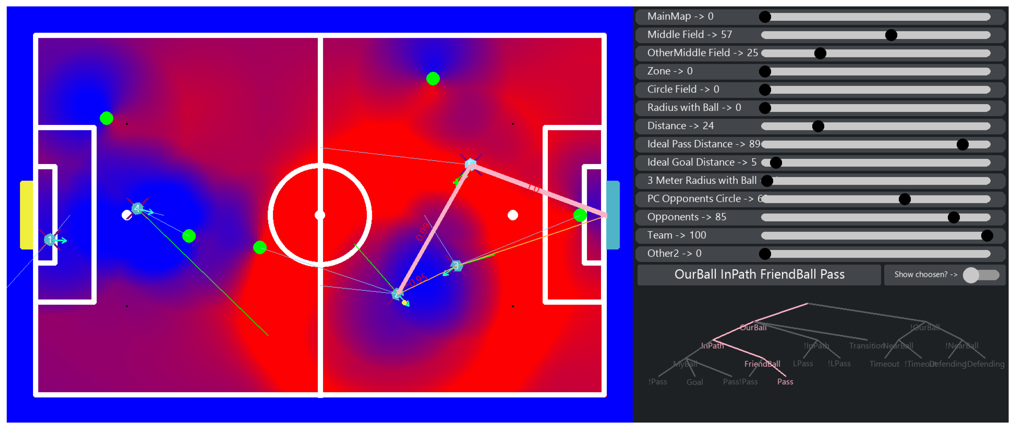
7.4. Map Fusion
7.5. Calibration
8. Simulator
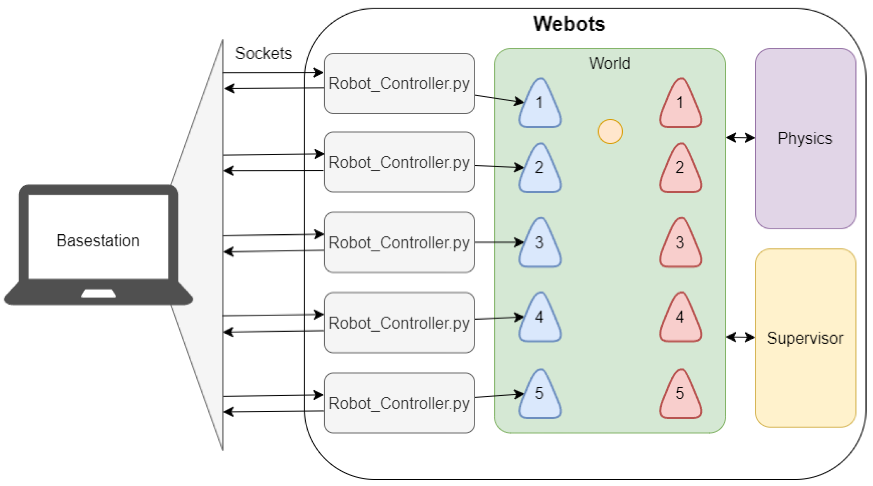
8.1. Architecture
8.2. Simulator Elements
8.2.1. Field, Goals, and Ball
8.2.2. Robot
8.2.3. Opponent
8.3. Communications System
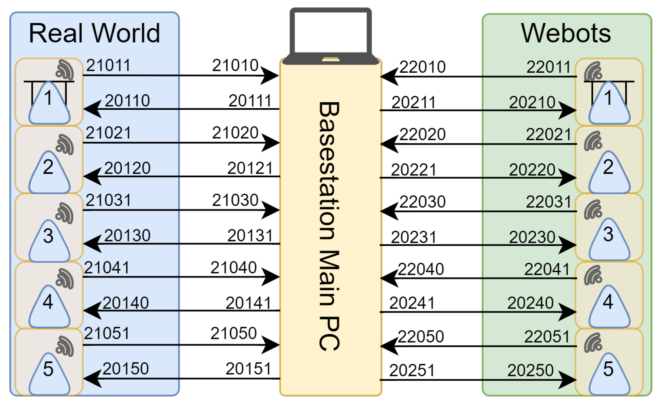
8.3.1. IPs
8.3.2. Web Sockets
8.4. Real-World Required Adaptations
9. Results
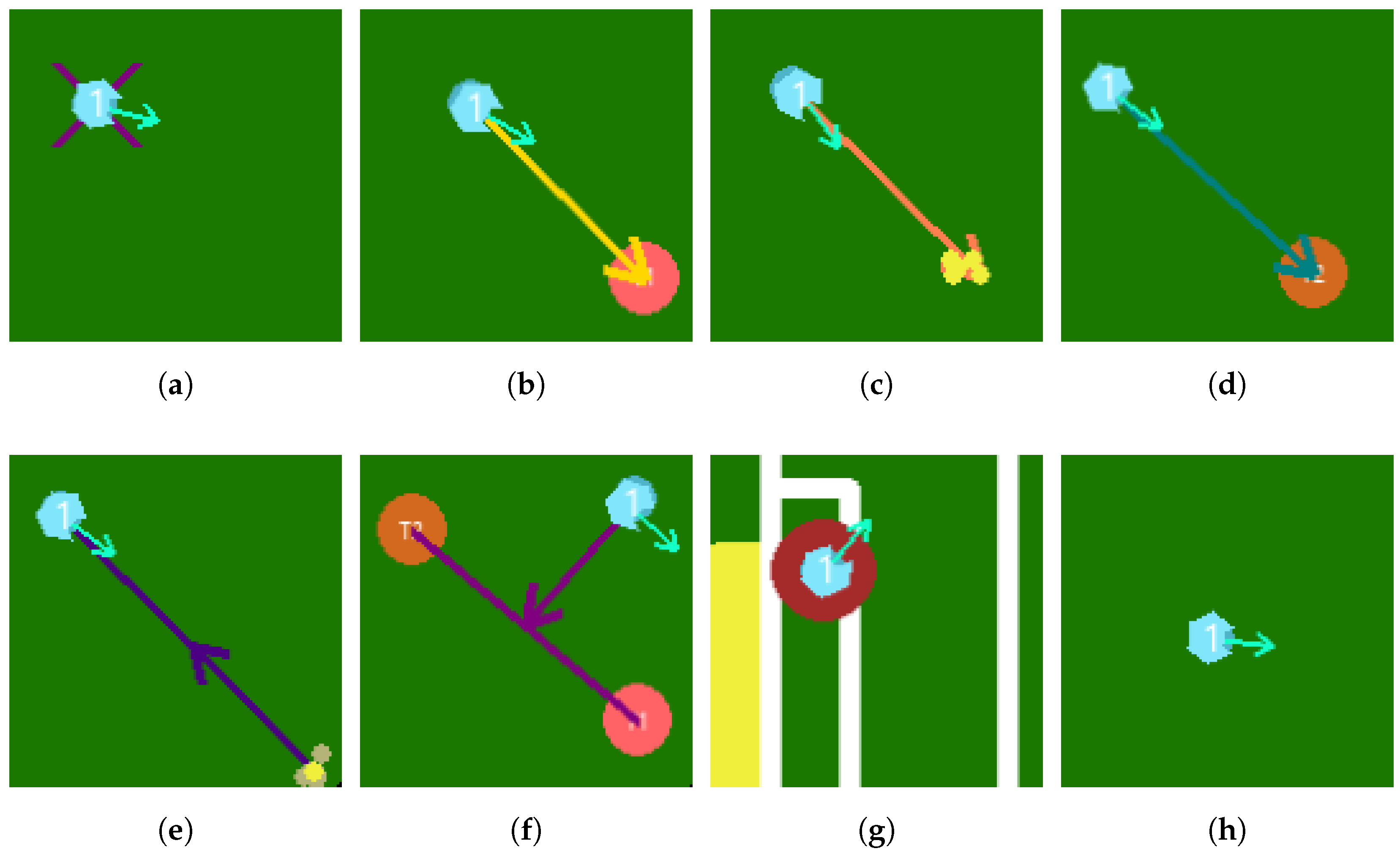
9.1. Simulator
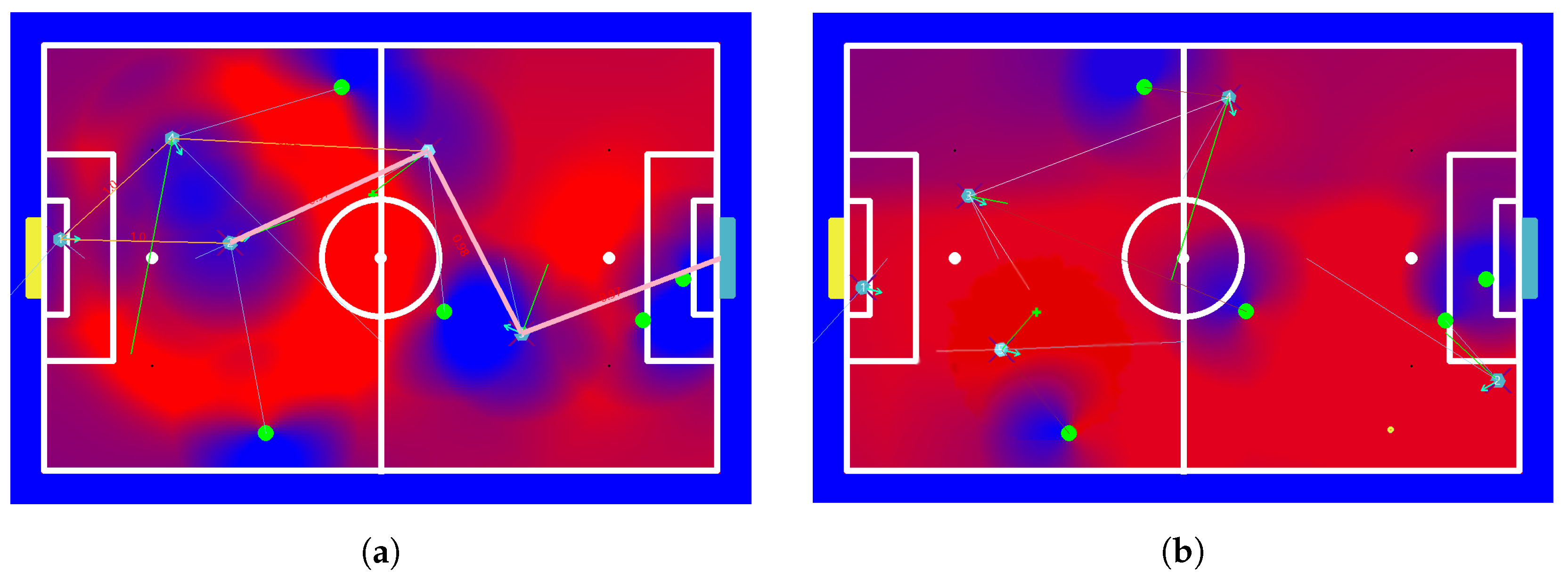
9.1.1. Case 1
9.1.2. Case 2
9.1.3. Case 3
9.1.4. Case 4
9.2. Against Humans
9.3. Real World
9.3.1. Play 1
9.3.2. Play 2
9.3.3. Play 3
9.3.4. Play 4
9.3.5. Real-World Differences
10. STP vs. PBS
10.1. Differences
10.2. Limitations
10.3. Modularity, Flexibility, and Scalability
11. Conclusions
- Manually positioning an opponent;
- Strategy vs. manually controlled by the base station;
- Strategy vs. humans controlling the opponents with gamepads.
Author Contributions
Funding
Data Availability Statement
Acknowledgments
Conflicts of Interest
Appendix A. “LAR@MSL Strategy: Humans vs. Robots in the Simulator”
Appendix B. “LAR@MSL Strategy: RoboCup Plays”
References
- Nardi, D.; Noda, I.; Ribeiro, F.; Stone, P.; von Stryk, O.; Veloso, M. RoboCup Soccer Leagues. AI Mag. 2014, 35, 77–85. [Google Scholar] [CrossRef]
- Ribeiro, A.; Costa, J.; Martins, J.; Silva, R.; Lima, R.; Lopes, C.; Lopes, G.; Ribeiro, A.F. LAR@MSL Description Paper 2023. Available online: https://lar.dei.uminho.pt/images/downloads/LAR@MSL_TDP%202023.pdf (accessed on 13 October 2023).
- Stone, P. Will Robots Triumph Over World Cup Winners by 2050? Available online: https://spectrum.ieee.org/robocup-robot-soccer (accessed on 28 October 2023).
- Mendoza, J.P.; Biswas, J.; Zhu, D.; Wang, R.; Cooksey, P.; Klee, S.; Veloso, M. CMDragons 2015: Coordinated Offense and Defense of the SSL Champions. In RoboCup 2015: Robot World Cup XIX. RoboCup 2015; Almeida, L., Ji, J., Steinbauer, G., Luke, S., Eds.; Lecture Notes in Computer Science; Springer: Cham, Switzerland, 2018; Volume 9513. [Google Scholar] [CrossRef]
- Biswas, J.; Mendoza, J.P.; Zhu, D.; Choi, B.; Klee, S.; Veloso, M. Opponent-driven planning and execution for pass, attack, and defense in a multi-robot soccer team. In Proceedings of the AAMAS ’14: International conference on Autonomous Agents and Multi-Agent Systems, Paris, France, 5–9 May 2014; Volume 1, pp. 493–500. [Google Scholar]
- Browning, B.; Bruce, J.; Bowling, M.; Veloso, M. STP: Skills, tactics, and plays for multi-robot control in adversarial environments. Proc. Inst. Mech. Eng. Part J. Syst. Control Eng. 2005, 219, 33–52. [Google Scholar] [CrossRef]
- De Koning, L.; Mendoza, J.P.; Veloso, M.; van de Molengraft, R. Skills, Tactics and Plays for Distributed Multi-robot Control in Adversarial Environments. In RoboCup 2017: Robot World Cup XXI. RoboCup 2017; Akiyama, H., Obst, O., Sammut, C., Tonidandel, F., Eds.; Lecture Notes in Computer Science; Springer: Cham, Switzerland, 2018; Volume 11175. [Google Scholar] [CrossRef]
- Schwab, D.; Zhu, Y.; Veloso, M. Learning Skills for Small Size League RoboCup. In RoboCup 2018: Robot World Cup XXII. RoboCup 2018; Holz, D., Genter, K., Saad, M., von Stryk, O., Eds.; Lecture Notes in Computer Science; Springer: Cham, Switzerland, 2019; Volume 11374. [Google Scholar] [CrossRef]
- Orr, J.; Dutta, A. Multi-Agent Deep Reinforcement Learning for Multi-Robot Applications: A Survey. Sensors 2023, 23, 3625. [Google Scholar] [CrossRef]
- Antonioni, E.; Suriani, V.; Riccio, F.; Nardi, D. Game Strategies for Physical Robot Soccer Players: A Survey. IEEE Trans. Games 2021, 13, 342–357. [Google Scholar] [CrossRef]
- Wu, J.; Snášel, V.; Cui, G. A Graph Theory-Based Evaluation of Strategy Set in Robot Soccer. In Intelligent Data Analysis and Its Applications, Volume I. Advances in Intelligent Systems and Computing; Pan, J.S., Snasel, V., Corchado, E., Abraham, A., Wang, S.L., Eds.; Springer: Cham, Switzerland, 2014; Volume 297. [Google Scholar] [CrossRef]
- Caputo, R.R.; Santos, E.B.d. Bayesian Classifiers Supported by Ranking for Decision Making in Robot Soccer. In Proceedings of the 2018 7th Brazilian Conference on Intelligent Systems (BRACIS), Sao Paulo, Brazil, 22–25 October 2018; pp. 432–437. [Google Scholar] [CrossRef]
- Budanov, D.; Feltracco, J.; Kamat, J.; Medrano, R.; Naeem, S.; Neiger, J.; Osawa, R.; Pan, M.; Peterson, E.; Shaw, A.; et al. RoboJackets 2017 Team Description Paper. Available online: https://ssl.robocup.org/wp-content/uploads/2019/01/2017_TDP_RoboJackets.pdf (accessed on 18 December 2023).
- Abe, T.; Orihara, R.; Sei, Y.; Tahara, Y.; Ohsuga, A. Acquisition of Cooperative Behavior in a Soccer Task Using Reward Shaping. In Proceedings of the 2021 5th International Conference on Innovation in Artificial Intelligence (ICIAI ’21), Xiamen, China, 5–8 March 2021; Association for Computing Machinery: New York, NY, USA, 2021; pp. 145–150. [Google Scholar] [CrossRef]
- Liu, S.; Lever, G.; Wang, Z.; Merel, J.; Eslami, S.M.A.; Hennes, D.; Czarnecki, W.M.; Tassa, Y.; Omidshafiei, S.; Abdolmaleki, A.; et al. From Motor Control to Team Play in Simulated Humanoid Football. Available online: https://arxiv.org/abs/2105.12196 (accessed on 23 October 2023).
- Tavafi, A.; Banzhaf, W. A hybrid genetic programming decision making system for RoboCup soccer simulation. In Proceedings of the Genetic and Evolutionary Computation Conference (GECCO ’17), Berlin, Germany, 15–19 July 2017; Association for Computing Machinery: New York, NY, USA, 2017; pp. 1025–1032. [Google Scholar] [CrossRef]
- Lima, P.; Bonarini, A.; Machado, C.; Marchese, F.M.; Marques, C.; Ribeiro, F.; Sorrenti, D.G. Omni-Directional Catadioptric Vision for Soccer Robots. Robot. Auton. Syst. J. 2021, 36, 87–102. Available online: https://hdl.handle.net/1822/3173 (accessed on 21 October 2023). [CrossRef]
- Middle Size Robot League Rules and Regulations for 2023. Available online: https://msl.robocup.org/wp-content/uploads/2023/06/Rulebook_MSL2023_v24.2.pdf (accessed on 21 October 2023).
- Quinlan, J.R. Induction of Decision Trees. Available online: https://hunch.net/~coms-4771/quinlan.pdf (accessed on 13 October 2023).
- Song, Y.Y.; Lu, Y. Decision tree methods: Applications for classification and prediction. Shanghai Arch. Psychiatry 2015, 27, 130–135. [Google Scholar] [CrossRef] [PubMed]
- Wang, Y.; Shenhan, J.; Chen, Z.; Huang, Z.; Xiong, R. Multi-Agent Collaboration for Feasible Collaborative Behavior Construction and Evaluation. 2019. Available online: https://www.researchgate.net/publication/336146890_Multi-agent_Collaboration_for_Feasible_Collaborative_Behavior_Construction_and_Evaluation (accessed on 28 October 2023).
- Santos, F.; Almeida, L.; Lopes, L.S.; Azevedo, J.L.; Cunha, M.B. Communicating among robots in the RoboCup Middle-Size League. Available online: https://sweet.ua.pt/lsl/pubs/CLI-2010-b-robocup09-final.pdf (accessed on 16 October 2023).
- Olthuis, J.J.; Beumer, R.M.; Bogaert, R.v.; Hameeteman, D.M.J.; de Loo, H.C.T.v.; G, M.J.; Molengraft, V.d.; Teurlings, P.; Verhees, E.D.T. Available online: https://msl.robocup.org/wp-content/uploads/2022/12/Risk_Evaluation_of_Robot_Soccer_with_Humans_in_MSL.pdf (accessed on 8 October 2023).
- O’Hagan, A. Bayesian Statistics: Principles and Benefits. Available online: https://edepot.wur.nl/134085 (accessed on 7 September 2023).
- Log Probabilities. Available online: https://chrispiech.github.io/probabilityForComputerScientists/en/part1/log_probabilities/ (accessed on 8 September 2023).
- Kass, R.E.; Vos, P.W. Geometrical Foundations of Asymptotic Inference; John Wiley & Sons: New York, NY, USA, 1997; p. 14. ISBN 0-471-82668-5. Available online: https://www.wiley.com/en-us/Geometrical+Foundations+of+Asymptotic+Inference-p-9780471826682 (accessed on 28 October 2023).
- Gowda, D.V.; Shashidhara, K.S.; Ramesha, M.; Sridhara, S.B.; Kumar, S.B.M. Recent Advances in Graph Theory And Its Applications. Adv. Math. Sci. J. 2021, 10, 1407–1412. [Google Scholar] [CrossRef]
- Ribeiro, F.; Moutinho, I.; Pereira, N.; Oliveira, F.; Fernandes, J.; Peixoto, N.; Salgado, A. High accuracy navigation in unknown environment using adaptive control. In Proceedings of the RoboCup 2007: Robot Soccer World Cup XI, Atlanta, GA, USA, 9–10 July 2007; Lecture Notes on Artificial Intelligence Series. Springer: Berlin/Heidelberg, Germany, 2017; Volume 5001, pp. 312–319. [Google Scholar] [CrossRef]
- Pereira, N.; Ribeiro, A.F.; Lopes, G.; Whitney, D.; Lino, J. Path planning towards non-compulsory multiple targets using TWIN-RRT*. Ind. Robot. Int. J. 2016, 43, 370–379. [Google Scholar] [CrossRef]
- FIFA Futsal Coaching Manual. Available online: https://cdn1.sportngin.com/attachments/document/000a-2348966/FIFA_futsal-coaching-manual.pdf (accessed on 6 October 2023).
- Kuhn, H.W. The Hungarian method for the assignment problem. Nav. Res. Logist. Q. 1995, 2, 83–97. [Google Scholar] [CrossRef]
- Barrett, P.; Hunter, J.; Miller, J.T.; Hsu, J.-C.; Greenfield, P. Matplotlib—A Portable Python Plotting Package. 2005. [Google Scholar]
- Ayala, A.; Cruz, F.; Campos, D.; Rubio, R.; Fernandes, B.; Dazeley, R. A Comparison of Humanoid Robot Simulators: A Quantitative Approach. Available online: https://arxiv.org/pdf/2008.04627.pdf (accessed on 20 October 2023).
- Korber, M.; Lange, J.; Rediske, S.; Steinmann, S.; Gluck, R. Comparing Popular Simulation Environments in the Scope of Robotics and Reinforcement Learning. Available online: https://arxiv.org/pdf/2103.04616.pdf (accessed on 20 October 2023).
- Webots Reference Manual R2023b: Supervisor. Available online: https://cyberbotics.com/doc/reference/supervisor (accessed on 20 October 2023).
- Crystal, S. Exclusive Comparison between WebSockets and gRPC. Available online: https://www.techunits.com/topics/architecture-design/exclusive-comparison-between-websockets-and-grpc/ (accessed on 20 October 2023).


| Skill | ID | A1 | A2 | A3 | A4 | A5 | A6 | A7 |
|---|---|---|---|---|---|---|---|---|
| Stop | 0 | - | - | - | - | - | - | - |
| Move | 1 | X | Y | - | - | |||
| Attack | 2 | P | - | - | - | - | ||
| Kick | 3 | - | - | |||||
| Receive | 4 | - | - | - | - | - | ||
| Cover | 5 | A | - | - | ||||
| Defend | 6 | - | - | - | - | - | ||
| Control | 7 | - | - | - |
| Variable Name | Meaning |
|---|---|
| Distance between robots | |
| Coordinate X from robot number i | |
| Coordinate Y from robot number i | |
| p | Constant factor to normalize the Bayesian curve between [0, 1] |
| d | Bayesian curve deviation—margin used for the ideal action distance |
| Best distance to action (pass or goal), ideal action distance between two robots, highest probability value | |
| totalProbability—action given probability | |
| totalProbability with the opponent’s influence | |
| Minimum distance from an opponent to the line of action (pass or goal) | |
| Maximum distance from where an opponent influences the action probability |
| Variable | Meaning |
|---|---|
| Ball | Team ball possession |
| Shoot | Team can perform a kick |
| Goal | Team is allowed by the rules to kick to the goal |
| Pass | Team can perform a pass |
| KnownBall | Team knows where the ball is |
| Free | The ball is free in the field with no nearby robot |
| OurBall | No ball possession but one of the teammates is the closest |
| Transition | The ball is in between an action, moving after a kick |
| Opponent | Opponent team has the ball or is the closest |
| Pass | The transition is a pass from our team |
| Goal | The transition is a goal kick |
| Variable | Meaning |
|---|---|
| OurBall | Team ball possession |
| InPath | Robot is in the ideal ball path |
| Transition | The ball is between actions |
| MyBall | Robot has the ball |
| FriendBall | A teammate has the ball |
| Pass | A pass can be performed |
| Goal | The next action is a kick to the goal |
| LPass | There are lines of pass available |
| NearBall | Robot is the closest to the ball |
| Timeout | Timeout to attack the robot with the ball |
| Defending | Robot is defending an opponent |
Disclaimer/Publisher’s Note: The statements, opinions and data contained in all publications are solely those of the individual author(s) and contributor(s) and not of MDPI and/or the editor(s). MDPI and/or the editor(s) disclaim responsibility for any injury to people or property resulting from any ideas, methods, instructions or products referred to in the content. |
© 2023 by the authors. Licensee MDPI, Basel, Switzerland. This article is an open access article distributed under the terms and conditions of the Creative Commons Attribution (CC BY) license (https://creativecommons.org/licenses/by/4.0/).
Share and Cite
Ribeiro, A.F.A.; Lopes, A.C.C.; Ribeiro, T.A.; Pereira, N.S.S.M.; Lopes, G.T.; Ribeiro, A.F.M. Probability-Based Strategy for a Football Multi-Agent Autonomous Robot System. Robotics 2024, 13, 5. https://doi.org/10.3390/robotics13010005
Ribeiro AFA, Lopes ACC, Ribeiro TA, Pereira NSSM, Lopes GT, Ribeiro AFM. Probability-Based Strategy for a Football Multi-Agent Autonomous Robot System. Robotics. 2024; 13(1):5. https://doi.org/10.3390/robotics13010005
Chicago/Turabian StyleRibeiro, António Fernando Alcântara, Ana Carolina Coelho Lopes, Tiago Alcântara Ribeiro, Nino Sancho Sampaio Martins Pereira, Gil Teixeira Lopes, and António Fernando Macedo Ribeiro. 2024. "Probability-Based Strategy for a Football Multi-Agent Autonomous Robot System" Robotics 13, no. 1: 5. https://doi.org/10.3390/robotics13010005