1. Introduction
Mobile robots have become increasingly prevalent in our modern world, playing vital roles in various applications, from manufacturing [
1] and logistics [
2] to healthcare [
3] and exploration [
4], with paramount importance in agriculture [
5] throughout the last decades. A fundamental aspect of a mobile robot’s functionality is its ability to navigate and maneuver effectively in its environment, and this capability hinges mainly on its steering mechanisms. In the context of mobile robots, navigation refers to how these machines control the vehicle’s position, speed, and attitude as a function of time [
6]. Guidance denotes establishing the desired trajectory from the robot’s current position to a final position, including the desired changes in linear speed, angular speed, and associated accelerations for following the desired trajectory [
7].
The navigation of mobile robots encompasses a wide range of technologies and techniques, drawing from disciplines such as robotics, control theory, computer vision, and artificial intelligence [
8,
9]. As mobile robots become more sophisticated and versatile, their navigation mechanisms continue to evolve, enabling them to operate autonomously and safely in a variety of environments and scenarios [
10]. Effective guidance is crucial for deploying robots in economic sectors such as agriculture, which this article focuses on.
Critical challenges in robot navigation, in general, and particularly in agriculture, are mapping, localization, path planning, obstacle detection, and tracking control [
11]. Building an accurate map of the environment (Mapping) is essential for navigation in an agricultural field; thus, robots must simultaneously map the environment while localizing themselves [
12]. Creating and updating maps in real time can be challenging, especially in dynamic or unstructured environments; another challenge is Localization: robots must accurately determine their position within an environment to prevent navigation failures [
13]. Localization methods often rely on sensors like Global Navigation Satellite System (GNSS) [
14], LIDARs [
15], or computer vision [
16], and each has its advantages and limitations. GNSS solutions are preferred for agriculture in open fields where GNSS-denied areas are rare; however, denied areas are relatively common when navigating entire farms.
Once a robot knows its position and has a map of the environment, it needs to plan a safe and efficient path to its destination while considering various factors like terrain, obstacles, and the robot’s capabilities. The module responsible for finding a path is a Path Planner, generally associated with the Path Supervisor [
17]. This module oversees the robot following the path defined by the planner and guarantees the fulfillment of the specifications, such as preventing collisions. The Planner generates the path according to the known obstacles, but new static and dynamic obstacles can appear in its environment. Therefore, robots need to perceive their surroundings accurately to detect obstacles and navigate around them. This involves challenges in sensor accuracy [
18], occlusion handling [
19], and the ability to distinguish between static and moving obstacles [
20]. The Obstacle Detection System guarantees these activities. Finally, the robot needs a Tracking Controller to ensure an accurate following of the trajectory defined by the planner.
Controlling these two key aspects (planning and tracking) is challenging due to nonlinear robot dynamics, noise in perception systems, ground disturbances, and several unidentified parameters [
21]. The developed methods include classic Proportional-Integral-Derivative (PID) methods [
22], sliding mode controllers (SMC) [
23], flatness-based algorithms, optimal linear-quadratic techniques [
24], backstepping-based strategies [
25], optimal preview controllers [
26], and optimization-based methods [
27].
Selecting an appropriate control algorithm can be challenging since the performance of different techniques can vary depending on the situation. In the last decade, several studies have compared different control methodologies. For instance, fuzzy controllers were compared with PID controllers in [
28], several robust controllers were contrasted in [
29], predictive methods were compared with Linear Quadratic methods in [
30], the Linear Quadratic technique was confronted with the sliding mode in [
31], and kinematic-based algorithms were studied in [
32]. However, these studies did not reflect the performance of controllers in real-world situations with unexpected disturbances. In [
33], the authors compared trajectory tracking controllers under disturbances and sensor noise, but they only reported the comparison of two flatness-based controllers.
In more recent work, Zhu et al. [
34] developed a comparative study and validation of multiple control architectures of a small skid-steer mobile robot in an orchard. The study consisted of comparing a Proportional-Derivative (PD) controller with (i) a SMC controller, (ii) a Control Lyapunov Function (CFL), (iii) a Nonlinear Model Predictive Control (NMPC), (iv) a Tube-Based Nonlinear Model Predictive Control (TBNMPC), and (v) a Model Predictive Sliding Mode Control (MPSMC). It was shown that the SMC and TBNMPC controllers exhibited greater resilience against varying disruptions during both wide and narrow maneuvers. Moreover, the authors analyzed an Integral Absolute Error (IAE) that shows that the MPSMC had the overall lowest actuation effort; although it was only about 5% of an improvement compared to the PD controller. It should be noted that the authors use the same control laws to follow both straight and curved lines, and it is expected that the rest of the strategies will surpass the performance of the PD controller.
In summary, most comparative works are performed under controlled situations or in simulation and do not represent a viable solution, especially in applications in an agricultural domain where the environmental conditions and the configuration of the robotic system are highly variable. The experience with developing guidance controllers [
35] and control architectures [
36] indicates that classical solutions can solve the guidance problem in this type of condition and for the application studied in this work. Therefore, selection based on previous theoretical and experimental studies is advisable. Furthermore, the practical comparison is ineffective when selecting guiding algorithms for real robot applications due to time and cost.
This work presents an autonomous robot Guiding Manager for laser-based weeding in agriculture that encompasses a Local Planner and Supervisor, an Obstacle Detection System, and a Tracking Controller to guide the autonomous robot. The proposed approach was implemented on a mobile platform to configure a fully autonomous robot in charge of performing selective high-power laser treatment for weed control in maize, sugar beet, and wheat fields and was exhaustively validated in real operating conditions over 9 months in 3 different experimental farms. Thus,
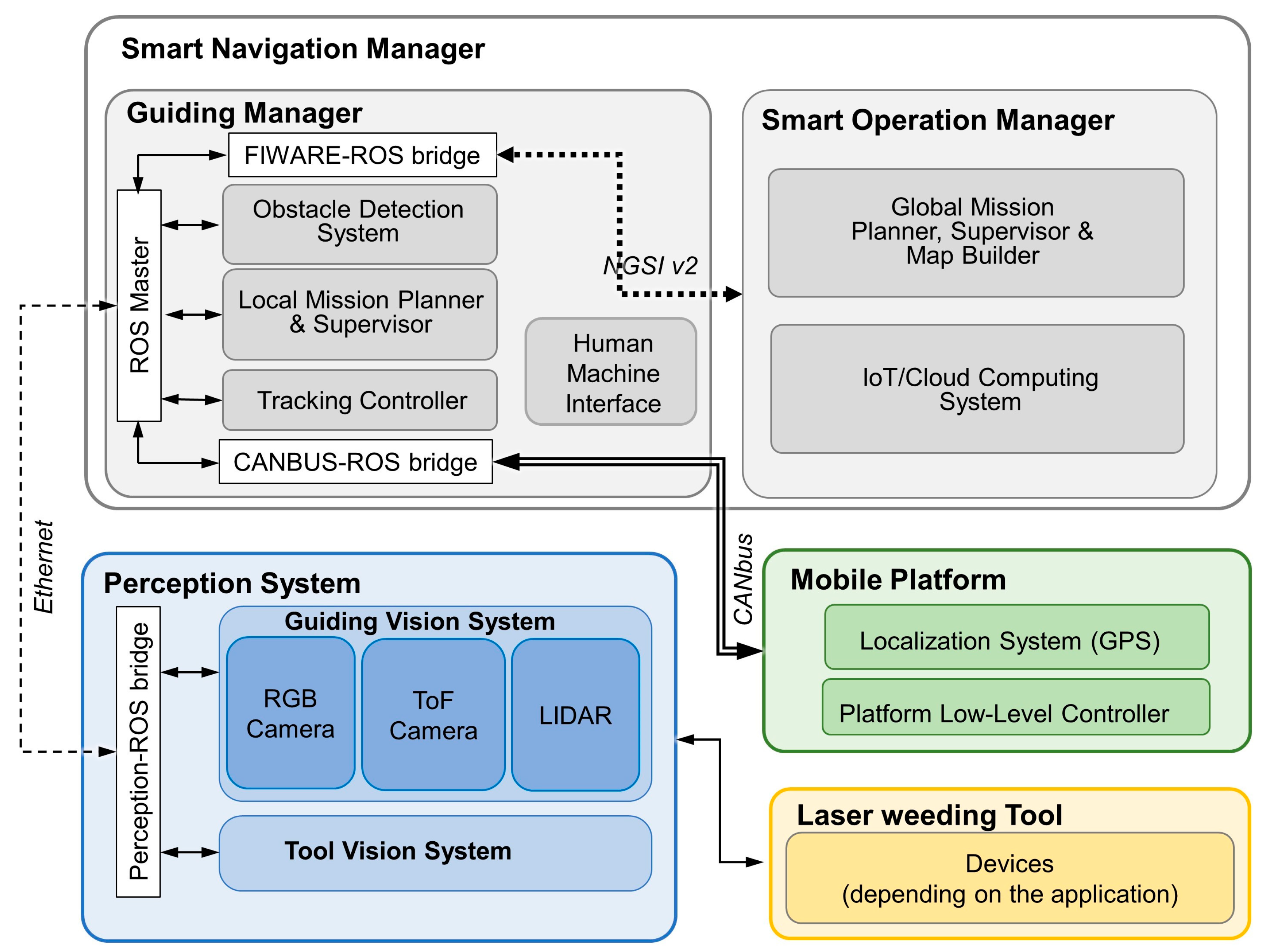
Section 2 presents the vehicle and sketches the Smart Navigation Manager that contains the Guiding Manager, which is given in
Section 3.
Section 4 describes the tests in a real farm to validate the algorithms in a specific agricultural task. Finally,
Section 5 summarizes the results, and
Section 6 presents the most relevant conclusions.
3. The Guiding Manager
This work focuses on the description and assessment of the Guiding Manager, which consists of the Local Planner and Local Supervisor, the Obstacle Detection System, and the Steering Controller.
3.1. Local Planner and Supervisor
These modules allow the development of a mission to be planned and supervised locally at a robot level. Given a user-defined mission or command, this module defines how to achieve (execute) that command. It considers the robot’s current position and the command’s final objective (including the intermediate goals that constitute the mission) and calculates the appropriate trajectories and behaviors to achieve the final point. This module integrates both absolute localization (through GNSS) and relative localization (odometry), and from the planning and navigation point of view, the system decides to use one localization method or the other on its own.
Within local planning, two fundamental strategies were developed:
The trajectories generated by both planners are executed mainly by three main controllers (Lateral Controller, Spiral Controller, and Linear Speed Controller) detailed in the Tracking Controller section.
The tasks performed by the robot are mainly of two types:
Approximation and
Treatment. The development of these tasks is made up of the concatenation of the two planners (
GoToGoal and
LineFollowing). The supervisor defines which planner should be activated and is guided according to the task performance. Additionally, the supervisor monitors the task execution and reports malfunctions to the operator.
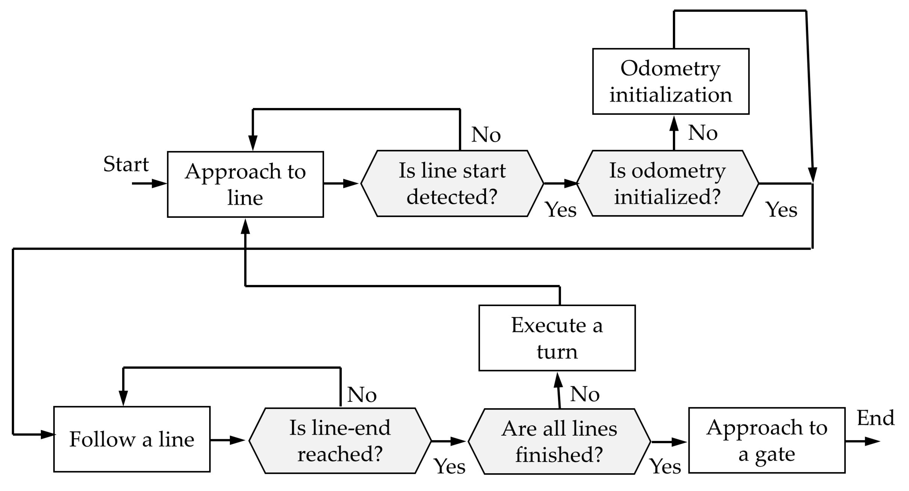
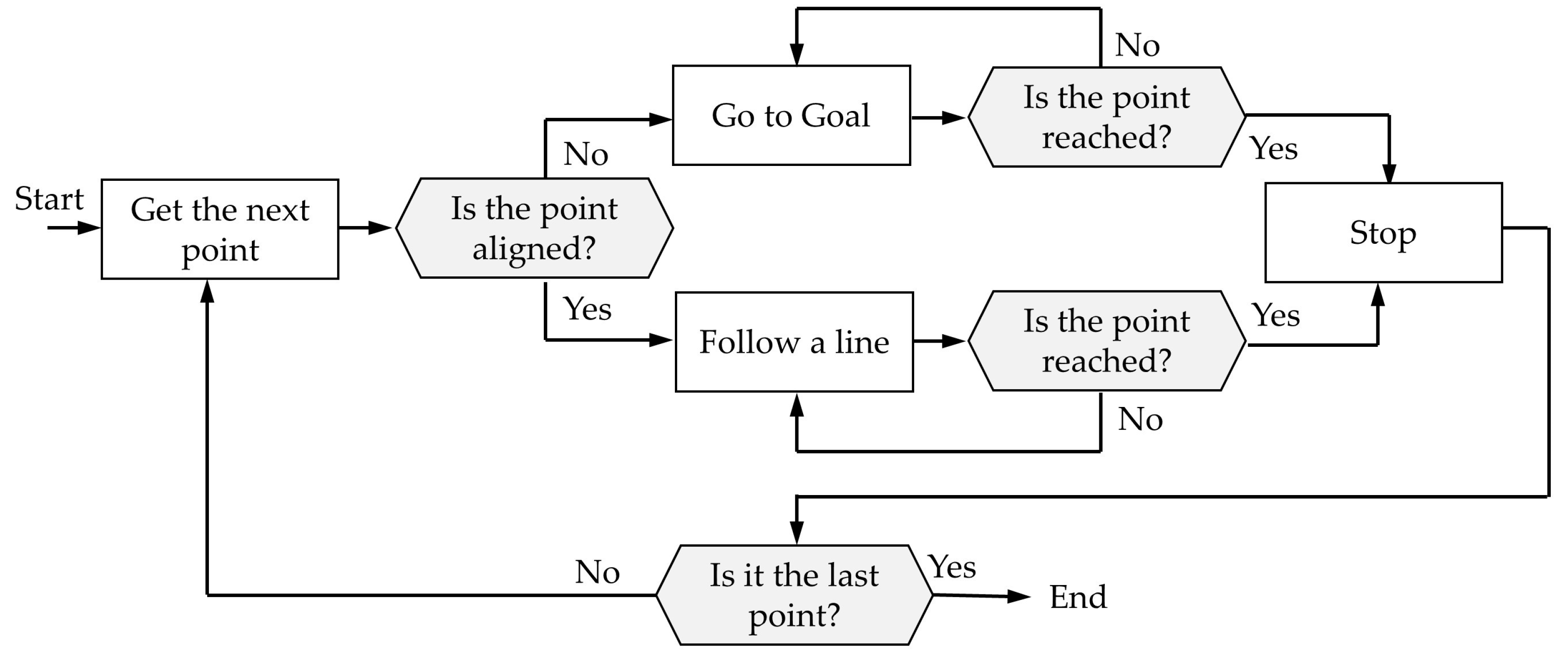
Figure 5 presents the state diagram of the execution of the
Treatment task, and
Figure 6 shows the diagram of the execution of the
Approximation task. Since the robot does not have sensors in the rear part, it is essential to avoid maneuvers that require moving backward; therefore, the turns to change crop rows in the field will be executed using the
GoToGoal planner.
3.2. Obstacle Detection System
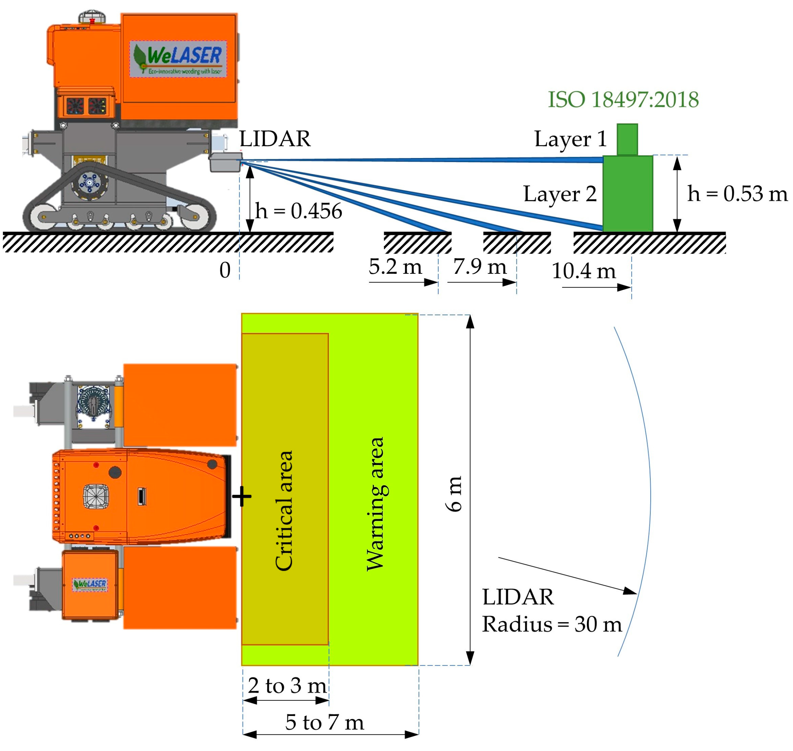
Given the vehicle’s characteristics and the application for which it is designed, only forward movement has been enabled. In this case, it is only necessary to have an obstacle detection system in the front part of the robot. Therefore, a LIDAR is used as the main sensor for obstacle detection. It is located in the front of the robot, just above the safety bumper (
Figure 7). The LIDAR comprises 4 layers (light beams) with a separation of 2.5 degrees between them. The LIDAR has been arranged and flipped with a clearance of almost half a meter from the ground so that most of the light beams have contact with the ground and obstacles (
Figure 7). For obstacle detection, only layer 1 is used to identify the obstacles. This arrangement allows the obstacle defined in the ISO 18497:2018 [
44] standard to be detected (
Figure 7).
For the LIDAR point cloud filtering, an open-access library [
45] was integrated within the Guiding Manager, which returns the positions of the obstacles and classifies them in circles or segments. This strategy has proven itself to be very useful given that for this application, as indicated above, the use of common approaches such as occupational grids or potential fields were discarded. Therefore, a strategy was required to represent the detected obstacles in such a way that trajectories based on Dubin’s curves could be generated to avoid them.
Within the obstacle detection system, there are two main behaviors that the robot can perform based on the position of the obstacle concerning the robot (
Figure 8):
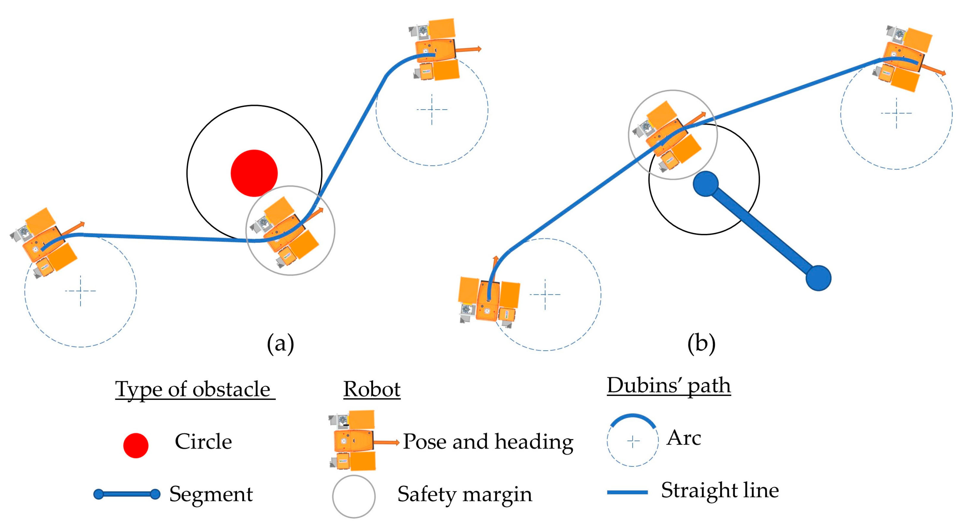
Regarding the methodology for avoiding obstacles, a trajectory planner is integrated to compute intermediate points in the planned trajectory if an obstacle is detected within the warning zone and on the robot’s trajectory. This trajectory planner takes advantage of the GoToGoal planner, which, as previously indicated, is based on Dubins’ paths. This guarantees that the shortest path between two points in an Euclidean plane can be established by concatenating arcs of a given radius and tangent straight lines.
During the missions, circumferences of equal and pre-defined radii are consistently applied to create the arcs. Since only the minimum robot turning radius is considered, the paths are always the shortest possible. Nonetheless, the variation in radius occurs when obstacles are detected (
Figure 8). When the obstacle detector provides the position and radius of a new obstacle in the collision range (warning area), a new waypoint for the path is entered into the calculation loop. If the obstacle is small enough, it will be represented by a Dubin’s circle equal to the radius of the obstacle plus a safety margin. If the obstacle is more significant, it will be represented by a straight segment defined by two ends. It is evaluated through which end of the path is shorter, applying a circle of radius equal to the robot’s minimum turning radius plus the safety margin. After avoiding the obstacle, the original goal point is recovered, continuing the path.
Figure 8.
Obstacle avoidance. (a) A trajectory avoiding a small obstacle; (b) a trajectory avoiding a large obstacle.
Figure 8.
Obstacle avoidance. (a) A trajectory avoiding a small obstacle; (b) a trajectory avoiding a large obstacle.
3.3. Tracking Controller
This module controls the mobile platform to track the trajectory computed by the Local Planner. Corrections to the platform’s trajectory are based on the difference between the desired position and orientation (pose) calculated by the Local Planner and the current platform’s pose, given by the GNSS.
Given that the two commonly followed trajectories in agricultural environments are straight lines and turns, the development of strategies oriented to the specific guidance of these trajectories is proposed. Therefore, three control laws were implemented: (a) Lateral Controller for straight paths, (b) Spiral Controller for curved paths, and (c) Linear Speed Controller for smoothing both (i) the start of guidance and (ii) the reaching the target point (
Figure 9). Each control law was implemented to execute the different types of planning.
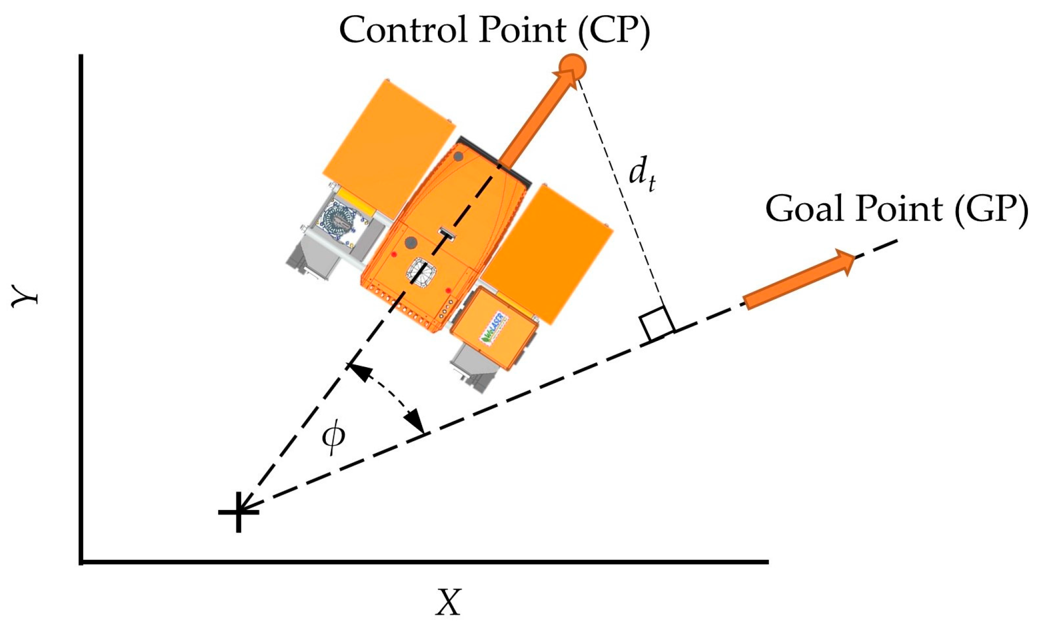
3.3.1. Lateral Controller
The lateral controller tries to bring the robot to the desired trajectory in position and orientation and move it at the desired speed,
vd, when the trajectory is achieved. To do this, the control law minimizes the distance,
dt, from the control point to the desired trajectory and the angle between the actual and desired trajectories,
ϕ, using a classic proportional-derivative (PD) controller in two variables: angular error (
ϕ) and lateral error (
dt). The robot’s control point,
CP, is located outside the robot’s body to facilitate its alignment with the desired trajectory (
Figure 9). The calculated variables are the robot’s angular speed around the z-axis,
ωs, and the robot’s linear speed along the
x-axis,
ls. The established control laws are as follows (
Figure 9):
That is, ws is proportional to ϕ and dt, where Kϕ and KPd are the proportional gains, respectively. dir is a parameter that depends on whether CP is on the left (dir = −1) or on the right (dir = 1) of the desired trajectory. Moreover, ∆dt represents the variation of dt between two consecutive time instants, and KDd represents the derivative gain.
ls is proportional to vd, where Kv is the proportional gain, and the term adapts ls to ws. That is, when ws is high, ls is decreased and vice versa, in a similar way to how car drivers behave. Kw also helps in tuning the proportional controller.
The control parameters were tuned empirically, adjusting the convergence times and minimizing the error in both control variables. The experiments were conducted from the threshold speed of the moving platform (0.1 m/s) to the maximum speed allowed by the ground conditions and the mechanical stiffness of the moving platform (0.8 m/s).
3.3.2. Spiral Controller
One of the frequent maneuvers carried out by autonomous robots when navigating crop fields is rotation, which can appear when tracking a trajectory or performing a U-turn at the end of a row to face the next. In this study, the controller proposed by [
46], based on a previous study by Boyadzhiev, 1999 [
47], was adapted to enable the robot to follow circles. This algorithm uses a spiral curve as a general solution for robot turns. As a circle is a spiral with specific parameters, this solution is applicable for generating the circles in the Dubins’ trajectories or circle U-turns. Spirals have demonstrated their value in path-planning tasks because their curvature changes proportionally along their arc length and have been used to generate continuous-curvature paths [
48,
49]. Although only a few applications have been given to them as control laws for tracking curvatures [
50], they can serve as a general solution acting as a control algorithm for the curvatures in the Dubins’ path.
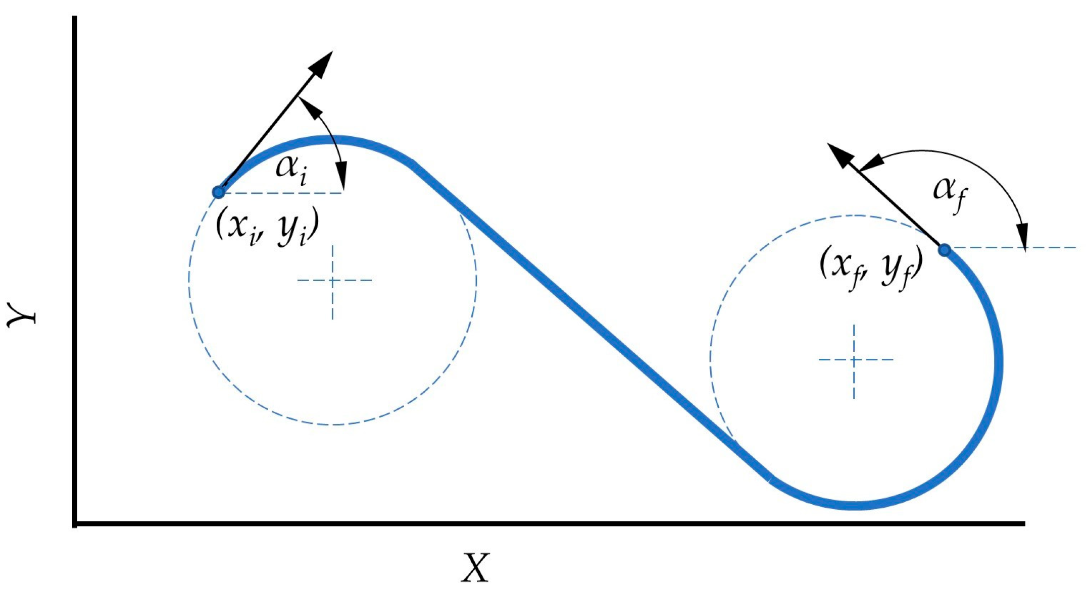
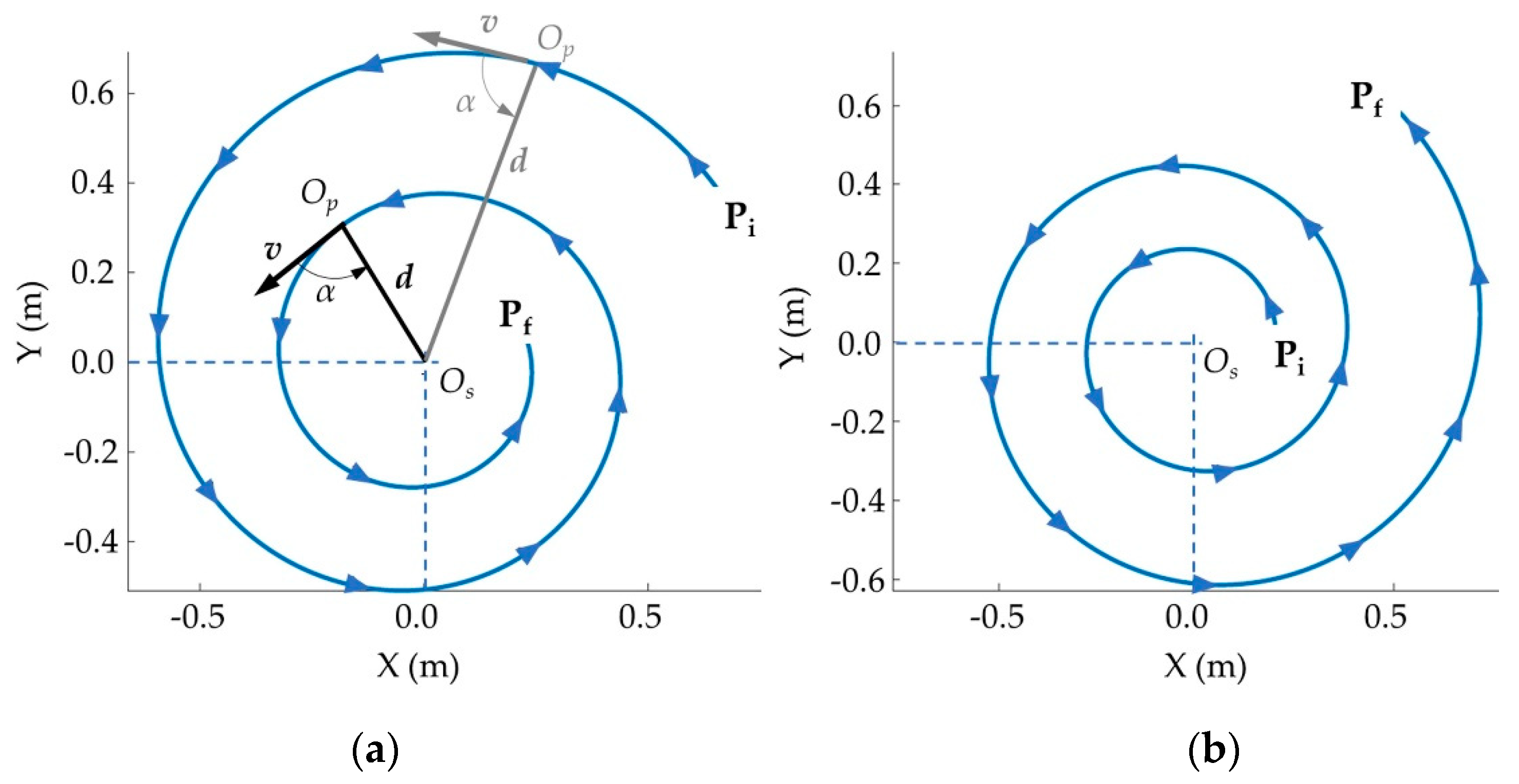
This method relies on the fact that a spiral is described as a trajectory followed by a point
Op moving on a plane concerning an invariant point
Os, spiral center (
Figure 10). Suppose
v is the velocity vector of
Op, (
v is tangent to the spiral trajectory) whose norm is represented as
v(
t). In this case,
d is the vector linking
Os to
Op with the norm
d(
t), and
α(
t) is the angle from
v to
d, then when
v(
t) and
α(
t) are constants (i.e.,
v(
t) =
vc and
α(
t) =
αc),
Op describes a spiral centered in
Os.
Therefore, a spiral is defined by an αc and a given d(0). The spiral behaves as follows:
- –
If 0 < αc < π, Op moves counter-clockwise concerning Os.
- –
If −π < αc < 0, Op moves clockwise.
- –
If 0 ≤
αc < π/2 or −π/2 ≤
αc < 0,
d(
t) diminishes with time (
Figure 10a), i.e.,
Op describes an inward spiral around
Os.
- –
If π/2 <
αc ≤ π or −π ≤
αc < −π/2,
d(
t) increases with time (
Figure 10b), i.e.,
Op describes an outward spiral around
Os.
- –
If αc = π/2 or αc = −π/2, d(t) = d(0), Op moves in a circle of radius d(0) around Os.
A method to follow a spiral involves creating a controller that guides the angle α(t) towards a desired angle αd. The value of αd determines whether the spiral is inward, outward, or circular. Once the robot has reached the spiral, it can either increase, decrease, or maintain its distance d(t) from the center of the spiral.
To build this controller, a constant desired linear velocity,
v(
t) =
vd, was imposed. Thus, the error is given as follows:
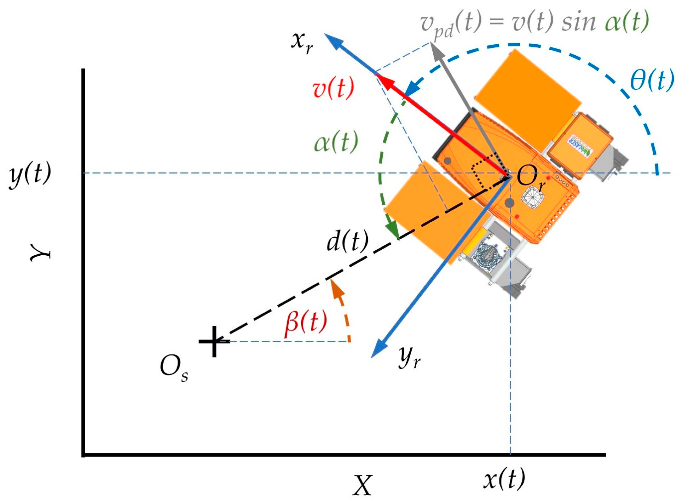
From
Figure 11, the relationship between the rotation angle (
θ) and the angle of the robot with respect to the fixed reference system (
β) is obtained:
Then
where
is the robot’s angular speed,
and
(
t) is the angular speed of
d, which is calculated by
where
is the
v(
t) component perpendicular to
d (
Figure 11), i.e.,
Finally, Equation (4) becomes
Therefore,
depends on
v(
t) and
ω(
t). However,
v(
t) is constant and known. Thus, the controller will focus only on controlling
ω(
t), i.e.,
Moreover, to make the error
e(
t) null, a controller proportional is defined. Thus, it follows that
This controller allows the robot to follow any spiral or circumference (different turning radius). In this case study, various turning radii were evaluated (between 0.75 m and 2 m), depending on the space available to make U-turns at the headlands of the crop fields. Moreover, for each mission, a predetermined turning radius was defined, which allows a minimum turn with adequate platform behavior. It should be noted that for a skid-steer platform to rotate about a designated center, it is necessary to select the angular and linear velocities. To always have both tracks moving forward, the turning radius must be greater than the distance between tracks. This behavior has been defined as desired to minimize the damage caused to the ground by tracks. Therefore, the nominal turning radius selection was determined based on the smooth behavior of the platform while turning and the available turning space.
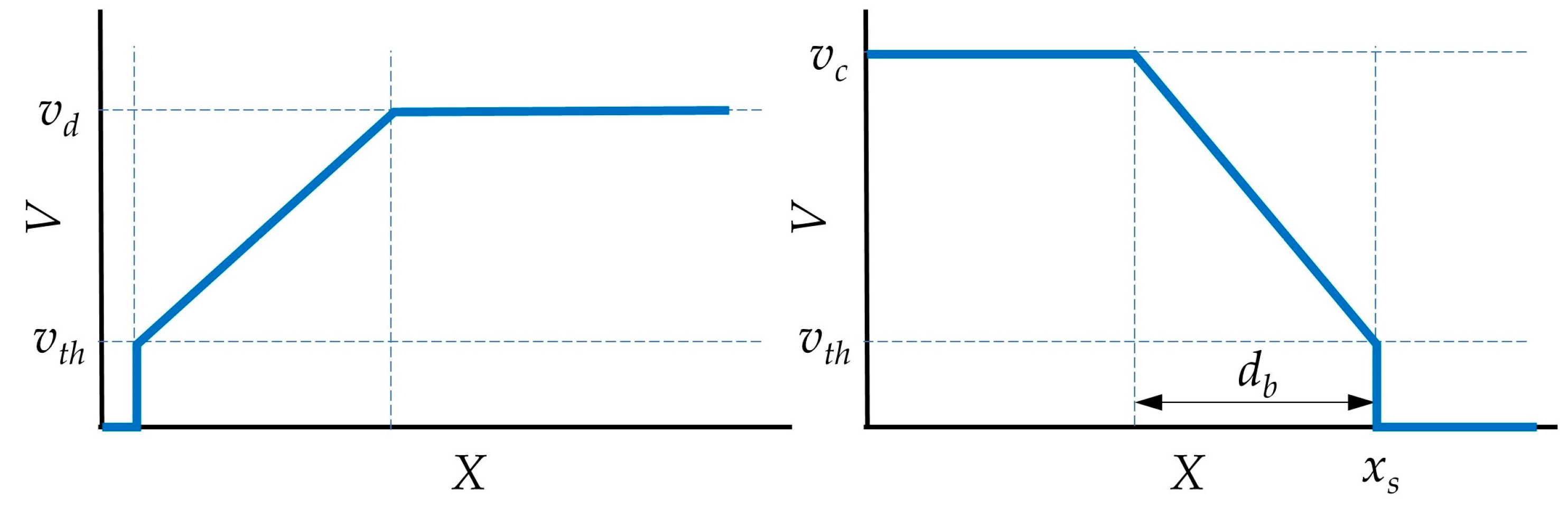
3.3.3. Linear Speed Controller
A linear speed controller is required to accelerate/decelerate the robot. A minimum threshold speed,
vth, was defined to stop the mobile platform without abrupt and fast maneuvers. Therefore, this controller calculates a linear speed profile from
vth to the desired final speed,
vd, when accelerating and a linear speed profile from the current speed,
vc, up to
vth when decelerating. After reaching
vth, the robot is ordered to stop.
Figure 12 illustrates the process when the robot must stop at
xs. The braking distance,
db, is the space the robot must travel to get
vth. It can be a fixed distance or a function of
vc. This simple controller is satisfactory for achieving proper linear speed features.
4. Testing the Guiding Manager
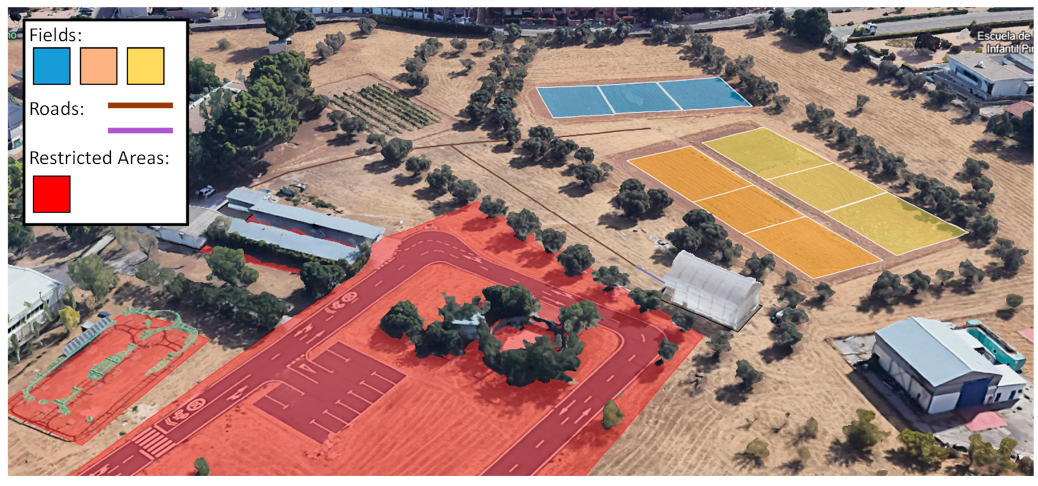
Several tests were conducted to validate the controllers and the implemented architecture from January to September 2023. The main tests were carried out in an experimental farm setup at the Centre for Automation and Robotics (CAR) in Madrid, Spain (40°18′45.166″ N, −3°28′51.096″ W). This experimental farm consists of a set of roads connecting the farm’s diverse elements, including buildings and crop fields (
Figure 13). To represent relevant field conditions, nine fields were configured, each with dimensions of approximately 20 m × 20 m, with headlands to perform the U-turns to change the crop rows of roughly 5 m. These fields were seeded with different crops, including maize, sugar beets, and wheat.
Moreover, during August 2023, further tests were carried out in two other experimental fields: (i) research facility Højbakkegaard (12°17′59.624″ N, 55°40′11.389″ W), belonging to the University of Copenhagen, in Taastrup, Denmark, during 17 and 18 August; and (ii) the farm Van den Borne Aardappelen, belonging to Van den Borne (5°10′32.241″ N, 51°19′12.298″ W), in Reusel, The Netherlands, during 23–26 August. In the farm in Denmark, two fields of approximately 40 m × 9 m were set up, one field seeded with maize and the second with sugar beet. On the other hand, on the farm in The Netherlands, two fields of maize and sugar beet were planted, with the first measuring roughly 37 m × 9 m and the second measuring about 37 m × 6 m.
The tests consisted of the robot executing a mission composed mainly of the abovementioned parts: (i) field
Approximation and (ii) field
Treatment. In the
Approximation stage, the robot started in some part of the farm, ordinarily close to the crop fields, and had to follow a set of geographical waypoints previously defined that allowed it to reach the beginning of the crop field. In some cases, these waypoints followed both dirt and asphalt roads. In certain situations, the terrain varied significantly: the experimental site in Spain had loose, stone-filled soil, while the fields in Denmark and The Netherlands were actual farms, offering more favorable ground conditions for the controllers. Additionally, humidity levels varied across different test scenarios, particularly during the experiments conducted in The Netherlands. Unfortunately, these soil conditions were not recorded, so in the analysis of the tests, it is impossible to carry out a characterization.
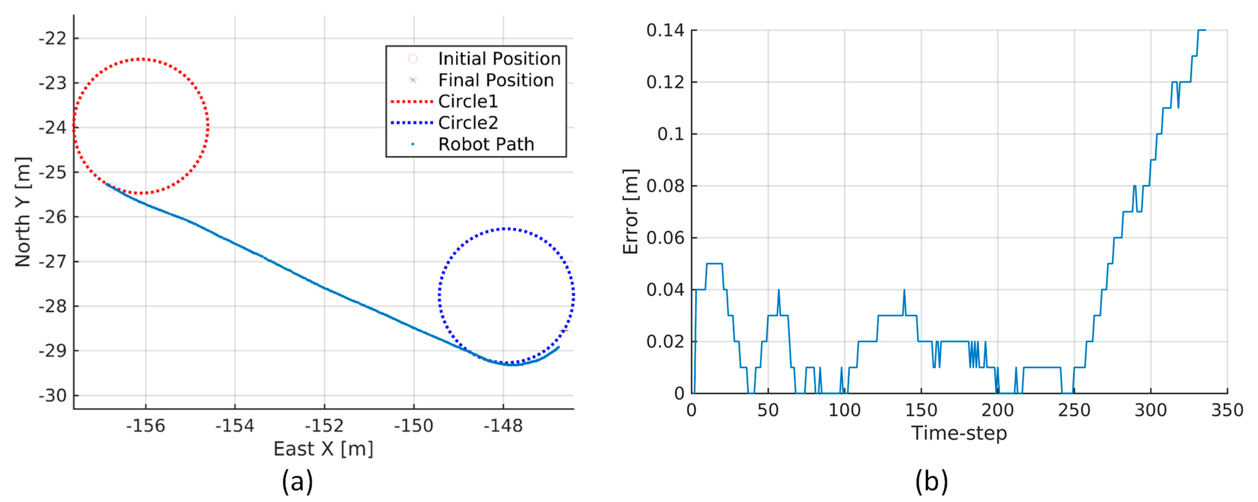
Figure 14a presents an example of the robot path executing an
Approximation task, which consists of reaching the starting point of the crop field. Moreover,
Figure 14b gives the corresponding lateral errors of the tracking action associated with both the Lateral and Spiral Controllers.
On the other hand, the
Treatment part represented the robot’s navigation in the crop field while performing some action/treatment. The positions of each crop row were known a priori, so a treatment map with complete coverage of the field was created, ensuring crop safety.
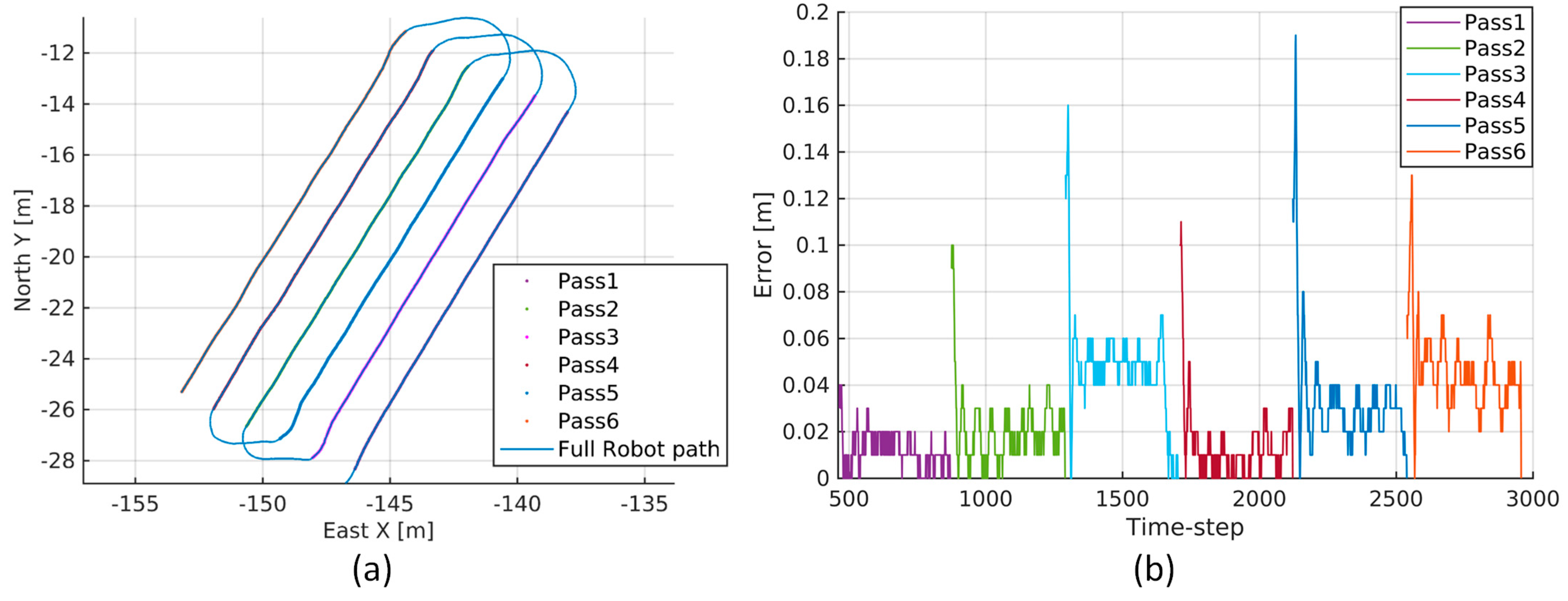
Figure 15a presents an example of the robot path following a
Treatment planning, which consists of 6 passes through the field, and their respective U-turns. Moreover,
Figure 15b presents the corresponding lateral errors of each pass associated with the lateral controller.
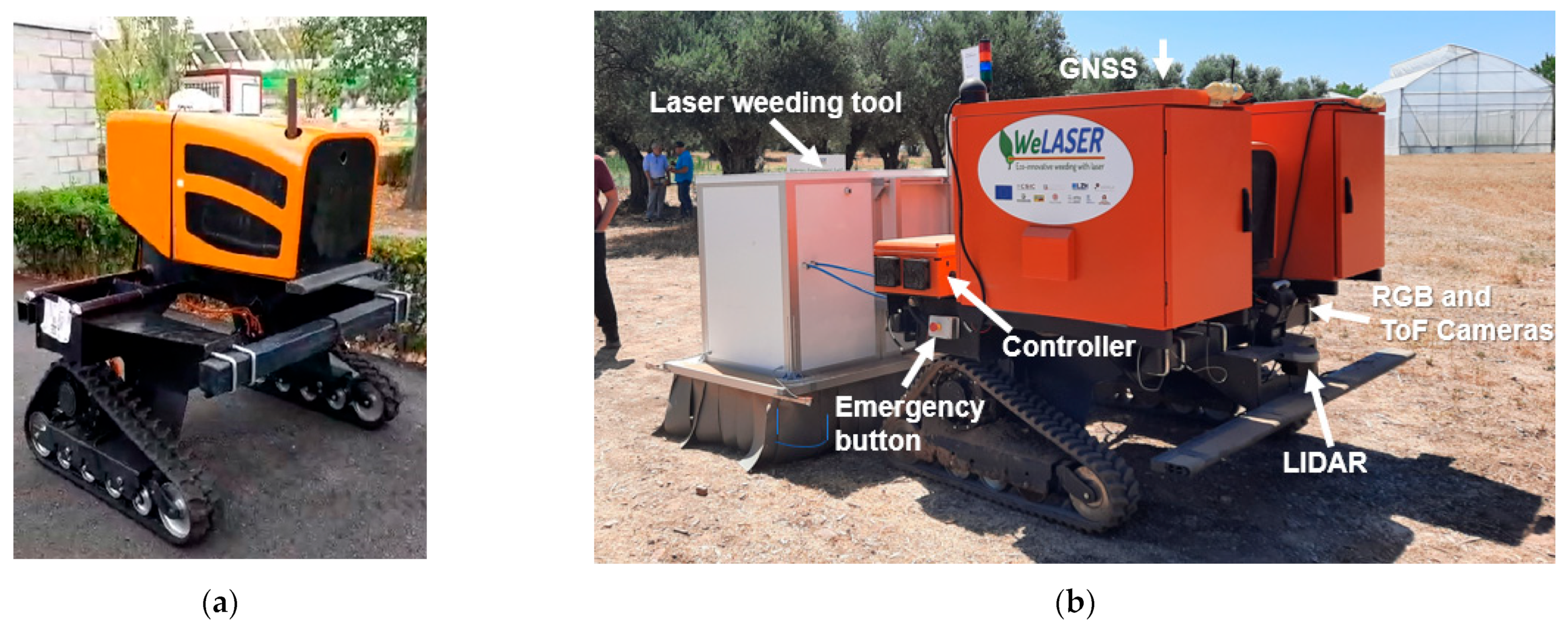
In this case study, the treatment corresponds to selective weed management through the use of a targeted high-power laser. In some tests, the high-power laser system was active and executing treatment. However, in most tests, the robot navigated without the high-power laser system being operational. In all tests, the robot carried the laser weeding tool (
Figure 1).
In both parts of the mission execution, the GoToGoal and the LineFollowing planners were used, depending on the robot’s task. During the Approximation stage, the following of the roads was mainly executed by the LineFollowing planner, even though the paths were not necessarily all straight. This is dependent on the condition that the lateral controller can adjust the robot’s position if the trajectory does not represent tight turns. On the other hand, in the presence of considerable changes in direction, which can be from 45 degrees, the GoToGoal planner was used. The nominal linear speed of the robot varied from 0.1 m/s to 0.8 m/s, depending on the different tests of the high-power laser system. In the turns, the robot was defined to go at a maximum linear speed of about 0.2 m/s.
The missions carried out included both approximation and treatment. Only missions with at least three passes or crossings through the crop field were selected, so 66 missions were analyzed. These missions correspond to a total operation time of approximately 13.4 h, with an average mission time of about 12 min. The total distance traveled by the robot in those 66 missions was about 9.3 km, where the LineFollowing planner was active, approximately 7.2 km, corresponding to 411 situations. In contrast, the GoToGoal planner only navigated about 2.08 km, related to 316 situations. This is mainly because the missions focused on navigation within the field. Therefore, the situations where the LineFollowing planner was activated corresponded to longer trajectories compared to short-turn trajectories planned by the GoToGoal planner. Furthermore, based on the characteristics of the robot and the weeding tool, which had a treatment width of about 1 m, the robot carried out navigation, performing treatment in 1 ha in total.
5. Results
To evaluate the performance of the controllers, three main measurements were executed:
The error when reaching the Goal Point (waypoint).
The average lateral error during the following of the planned trajectory.
The average angular error during the following of the planned trajectory.
The results obtained from these three indicators include the lateral, spiral, and speed controllers, which are presented as below.
5.1. Reach Error Results
As indicated above, the error obtained by the controllers when reaching the target point (Goal Point) was analyzed. In this case, the absolute reach error is defined as the Euclidean distance between the Goal Point and the longitudinal robot’s axis,
xr (
Figure 11). Moreover, in this case, the spiral and lateral controllers affect the error measurement of the linear speed controller, so the analysis is carried out jointly.
As indicated above, the robot’s localization system was based on GPS-RTK; its horizontal accuracy was about ±0.015 m, and its refresh frequency was around 10 Hz. These characteristics can affect the performance of the controllers in adequately identifying whether the Goal Point has been reached. Therefore, to maintain the robustness of the controllers, a parameter named distance threshold was defined, with a value of 0.05 m, slightly more than double the standard deviation of the localization system. This means that if a measured error was within this distance threshold, and the robot was behind the target point, this situation was defined as the target point reached. On the other hand, if the robot exceeds (passes over) the target point, the target point reached situation is automatically activated. Unfortunately, it could not be recorded every time the robot reached the Goal Point, whether it passed or was within that range.
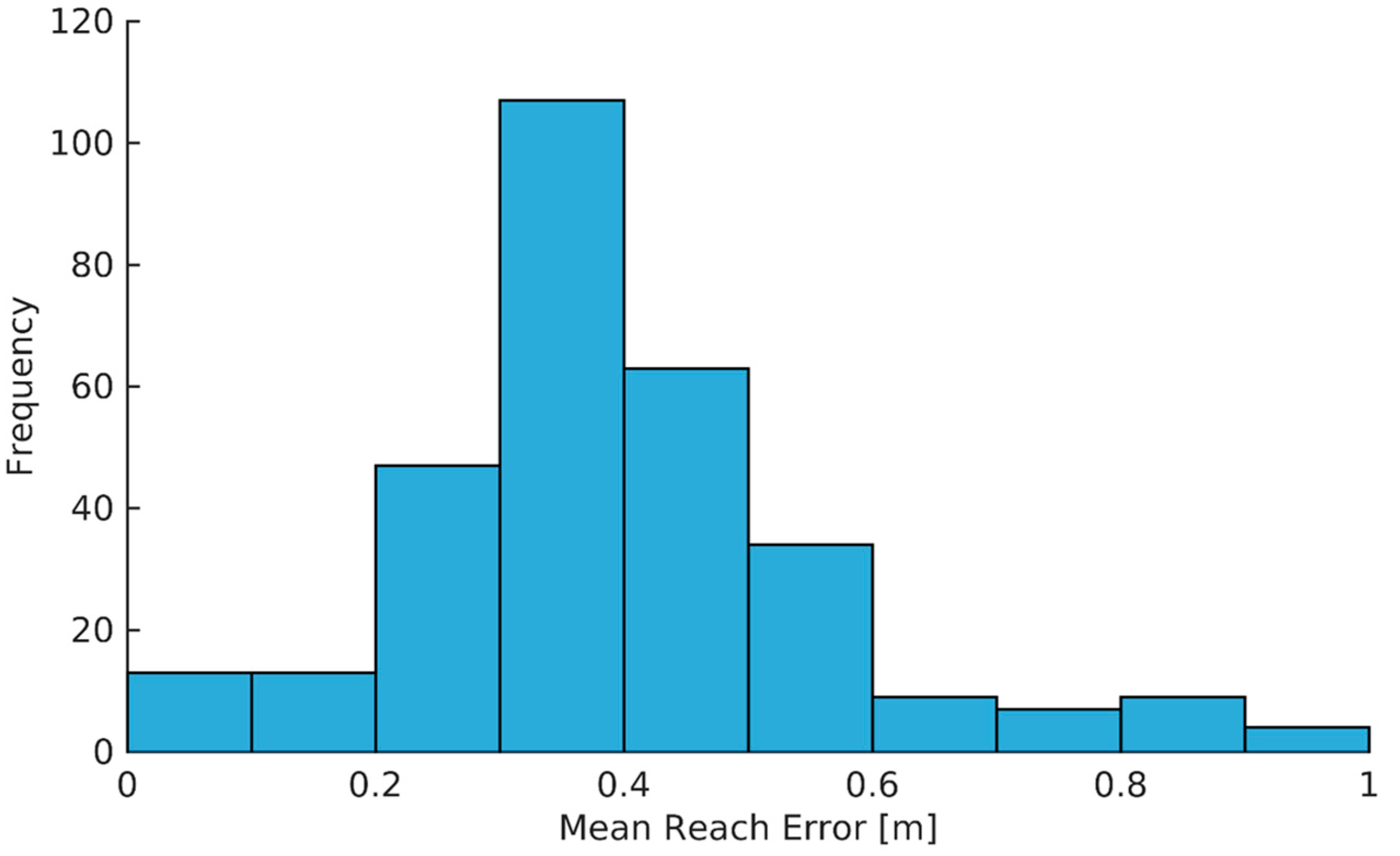
5.1.1. Reach Error of the Lateral Controller
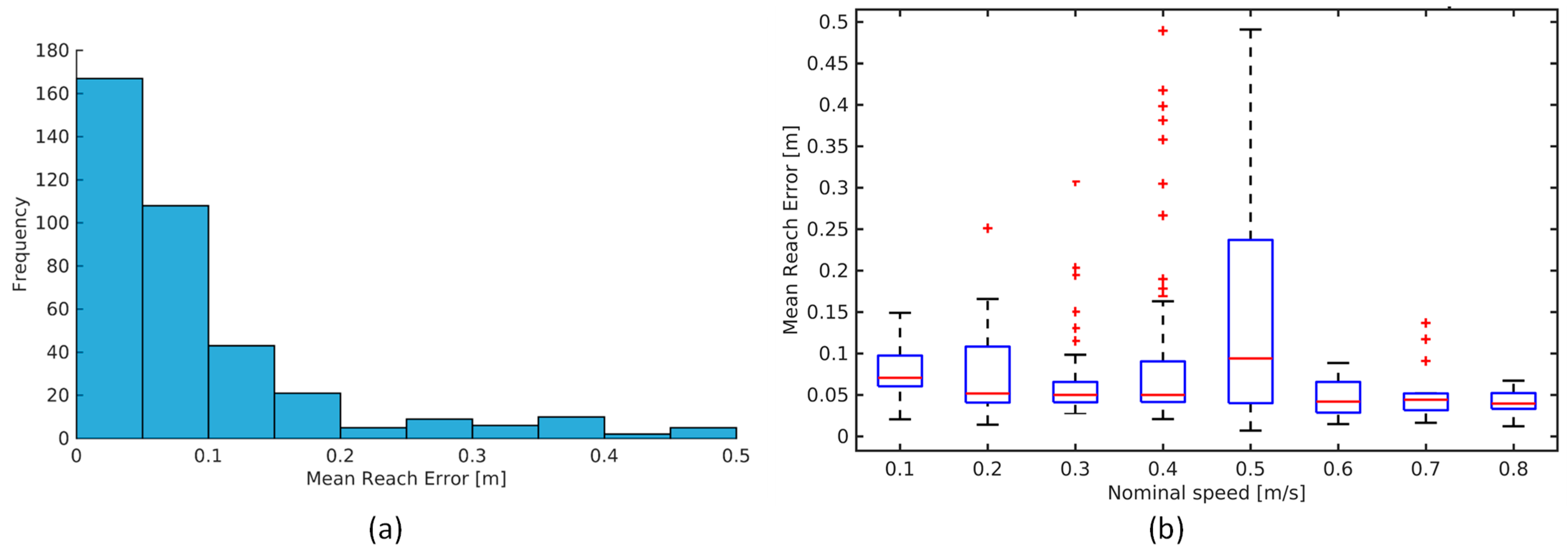
Figure 16a presents the histogram of the absolute error in all situations where the robot reaches its goal while following a linear path. In 8.3% of the cases, the absolute error was greater than 0.5 m. This is mainly because, in the tests carried out in some situations, the robot stopped because it was necessary for an operator to approach the robot or because the mission was aborted. By eliminating situations where the controller did not complete the
LineFollowing task, the absolute error in 44.4% of situations was less than 0.05 m, which corresponds precisely with the distance threshold. Moreover, in 73.1% of situations, the absolute error was less than 0.1 m. Even if the robot stops a few centimeters before or after the end of the crop line, it does not considerably affect the execution of the mission and the treatment. It should also be noted that these measurements were made while many other tests were performed on the robot, including tests to evaluate the high-power laser. During these tests, a mean reach error of approximately 0.09 m was achieved, with a horizontal accuracy of ±0.02 m.
Figure 16b presents a graph of the error concerning the nominal speed of the robot. The nominal speed is the maximum desired speed when following linear trajectories. In this box and whisker plot, the average error values for all speeds are below 0.1 m, most of which are close to 0.05 m. This means that regardless of the defined nominal speed, the linear speed controller effectively reduced the robot’s speed to get as close as possible to the target point. It should also be noted that the most significant errors are found between the nominal speeds of 0.4 m/s and 0.5 m/s, which correspond to 53.5% of the analyzed situations, given that this is the speed range desired by the high-power laser system to be profitable.
5.1.2. Reach Error of the Spiral Controller
Figure 17 presents the histogram of the absolute error in all situations where the robot reaches its goal while performing a turn, i.e., following a spiral. In 3.2% of the cases, the absolute error was greater than 1 m. This situation is similar to the one presented above. In some situations, the robot stopped either because it was necessary for an operator to approach the robot or because the mission was aborted. Moreover, in 20% of the situations, the controller stopped the robot at a distance between 0.5 m and 1 m from the goal point. These situations were expected since the controller sought to reach not only the target position but also the target orientation. The controller was defined so that it takes higher priority to arrive at the desired orientation even if the robot is far from the target. This means the robot reaches the target at an error distance of less than 0.5 m for 76.8% of the cases. For this controller, this is a splendid result, considering the robot’s dimensions. During these tests, a mean reach error of approximately 0.5 m was achieved, with a horizontal accuracy of ±0.02 m. This result contrasts considerably concerning the Lateral Controller, given that the execution of turns using a tracked robot in complex terrain conditions (presence of stones, loose or wet terrain, etc.) can generate this discrepancy without considering the robot’s dynamic model. In any case, these results were more than sufficient for the robot’s intended navigation capabilities.
5.2. Lateral Error Results
Another important indicator to evaluate the performance of the controllers, in particular the Lateral Controller and the Spiral Controller, is the lateral error in following the planned trajectory. At each instant of control time, i.e., when a new position value was obtained, the lateral error was calculated, which is one of the primary control variables of the presented controllers. Therefore, the lateral error is defined as the perpendicular distance between the robot and the trajectory point closest to the robot.
5.2.1. Lateral Error of the Lateral Controller
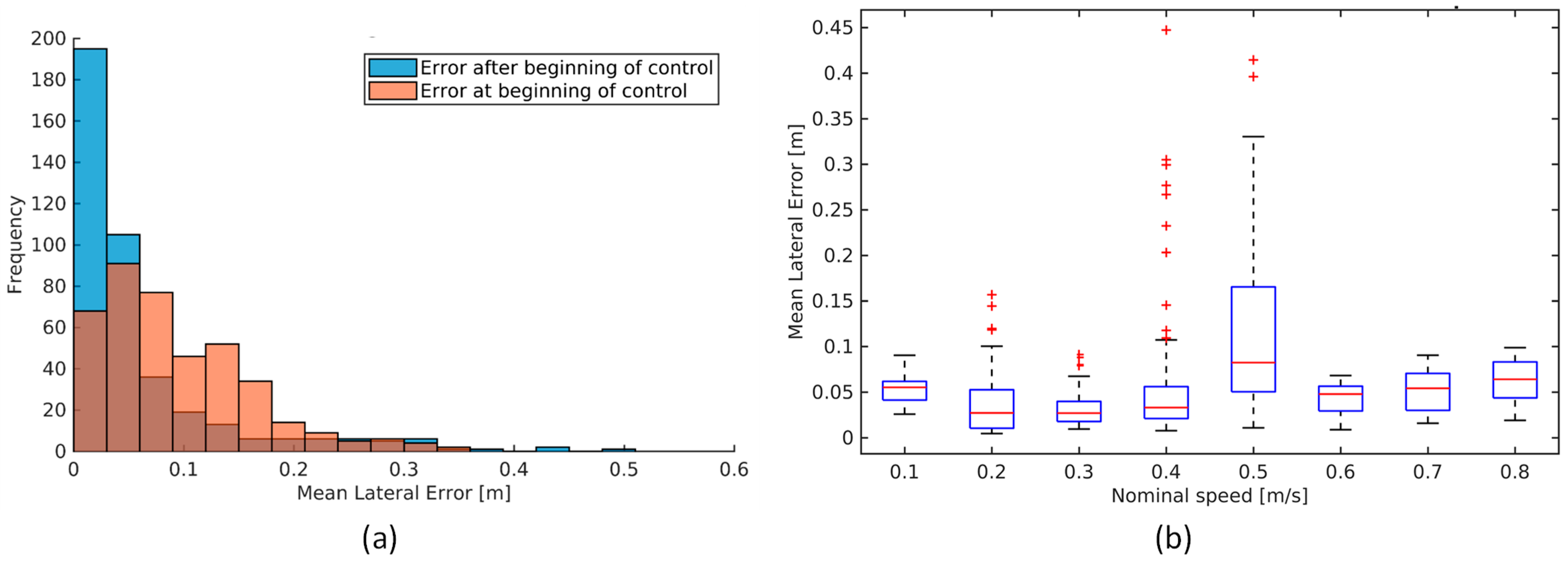
Figure 18a presents the histogram of the absolute lateral error in all situations where the robot follows a linear path. In this case, the average error of the complete trajectory is calculated each time a line has to be followed as a path. In 8.3% of the cases, the mean lateral error was higher than 0.5 m. This percentage coincides with the previous percentage of the reaching point error due to other factors unrelated to the development of the mission.
By eliminating those situations where the controller did not finish the following task, in 70% of the cases, the absolute error was less than 0.06 m. Moreover, in 79% of the situations, the absolute error was less than 0.09 m. It should be noted that this corresponds to the absolute lateral error. The situations where the error is greater is when the robot performs the maneuver to enter the crop lines, as illustrated in
Figure 16a, where after the beginning of the row following (after 20% of the path), 48% of the situations the absolute error is less than 0.03 m, while only the 17% of the situations the lateral error was below 0.03 m at the beginning of the mission. During these tests, a mean lateral error of approximately 0.076 m was achieved, with a horizontal accuracy of ±0.02 m. Moreover,
Figure 18b presents a graph of the lateral error concerning the nominal speed of the robot. This box and whisker plot represent a similar graph to the graph of the mean reach error concerning the nominal speed. Therefore, it should be noted that the error in reaching the Goal Point could correspond more to a lateral error than to a longitudinal error.
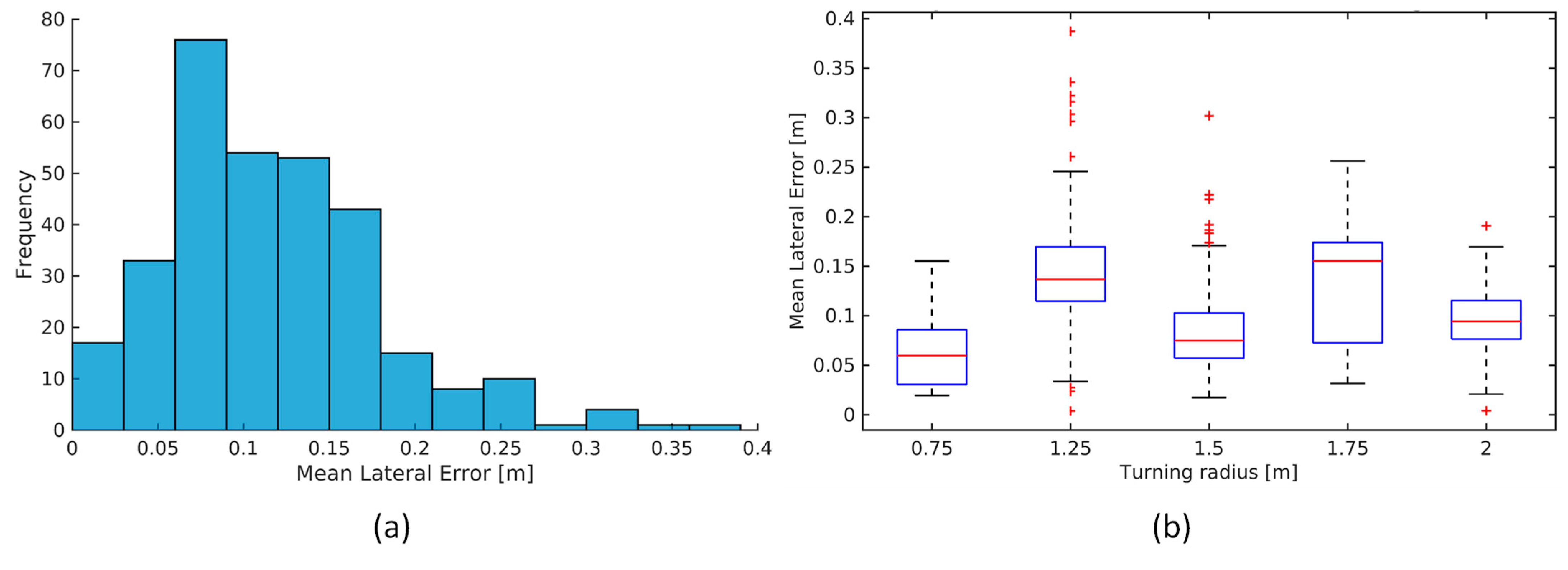
5.2.2. Lateral Error of the Spiral Controller
In the case of lateral error following the spirals, in 90.8% of the situations, the controller could keep the robot at a distance less than 0.2 m of the desired turning radius (
Figure 19a). Considering that the robot’s width is 1.48 m, maintaining a distance of 0.2 m when turning is more than satisfactory. An average of 0.12 m lateral error was obtained following the circle, with a horizontal accuracy of ±0.02 m. Moreover,
Figure 19b presents the averages of lateral errors achieved for different turning radii. These results demonstrate that the controller can adapt to different turning radii.
5.3. Angular Error Results
The angular error refers to the difference of the robot’s orientation vector (yaw angle) concerning the direction of the trajectory. Straight trajectories refer to the orientation in the Cartesian XY plane of the Goal Point, while spiral trajectories are the error between the orientation of the robot and the desired angle of rotation. In all tests, the spirals were configured with α = π; therefore, they represented circles.
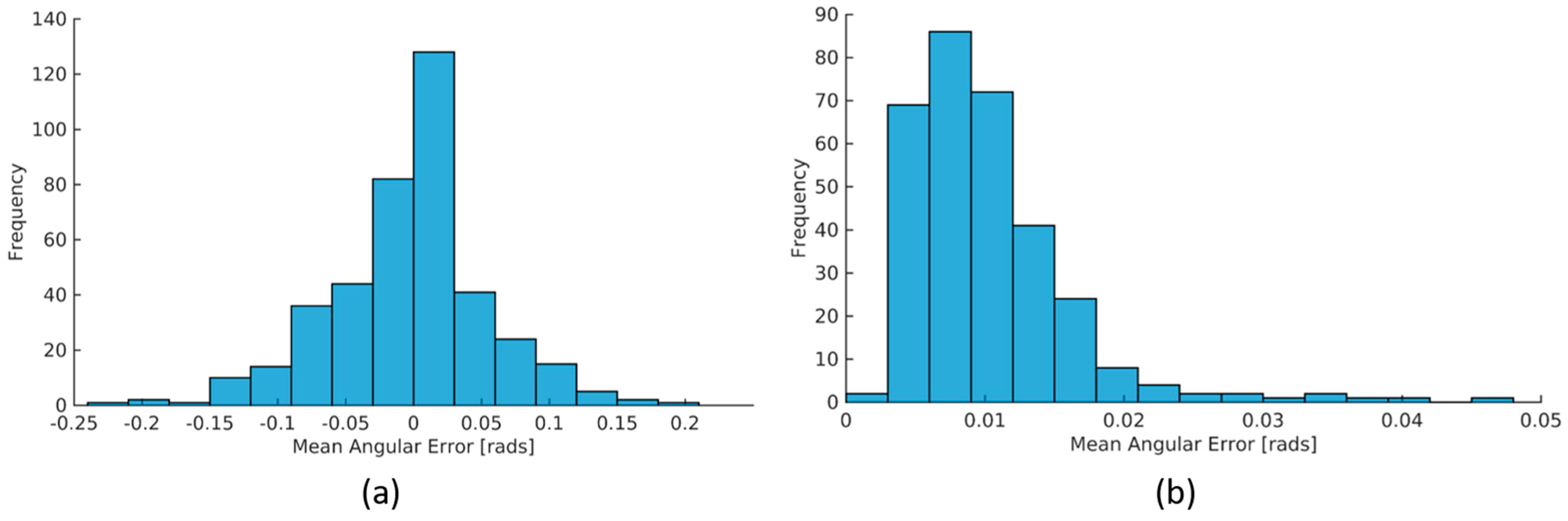
5.3.1. Angular Error of the Lateral Controller following a Straight Path
Figure 20a presents the histogram of the lateral error in all situations where the robot follows a straight path. Based on these data, a mean error of about −0.0033 rad was achieved, with a variance of about 0.0034 rad
2.
5.3.2. Angular Error of the Lateral Controller following a Spiral Path
Figure 20b presents the histogram of the lateral error in all situations where the robot follows a spiral path. A mean absolute error of about 0.0103 rad was achieved, with a variance of approximately 0.000035829 rad
2. In this case, the spiral controller presented a more stable behavior than the lateral controller, maintaining the rotation angle.
6. Conclusions
Control and guidance systems are essential elements of mobile robots for outdoor environments, particularly for agricultural landscapes, where ground conditions may be unfavorable due to rugged terrain, loose soil, excessive moisture, and stones, among other factors. This work presents a guidance manager based on a control architecture that allows the supervision of various controllers for tracking outdoor trajectories. The controllers developed mainly focus on straight and spiral trajectories separately, with the main purpose of enabling the autonomous navigation of a mobile platform that carries a specialized tool for selectively treating weeds using a high-power laser. The controllers are based on PID control laws that seek to always maintain not only the position of the robotic platform on the path but also its proper orientation, maintaining its integrity; this is especially essential for navigation in crop fields. The controllers were evaluated intensively over nine months, between January and September 2023, with a cumulative distance traveled of about 9.3 km and a total accumulated operating time of approximately 13.4 h, on different farms in Spain, Denmark, and Holland, thus demonstrating its ability to adapt to different scenarios, terrain, and situations.
The controllers were evaluated taking into consideration three key performance indicators: (1) the error in reaching the target point, (2) the average lateral error, and (3) the average angular error in tracking trajectories. For the first, both the lateral and spiral controllers affected the target’s reach error in conjunction with the linear speed controller. Therefore, the analysis was carried out together, obtaining a mean total error of about 0.09 m for the lateral controller and 0.5 m for the spiral controller. On the other hand, regarding the lateral error, a mean total error of approximately 0.076 m was obtained with the lateral controller, and a mean error of about 0.12 m for the spiral controller. Based on these tests, it is clear that the spiral controller performed worse than the linear controller, which is basically generated by the complex terrain conditions when making such tight turns that, in some cases, the turning radius was equal to or less than half the width of the robot. It was shown that the performance of the spiral controller was not affected by the desired turning radius but that this controller, like the lateral controller, was configured to prioritize maintaining the robot’s orientation (minimizing the angular error) by penalizing the lateral error. Therefore, the analysis of the angular error yielded excellent results.
It is important to emphasize that the decision to prioritize the minimization of the angular error is due to keeping the high-power laser tool aligned to the crop lines to perform an effective treatment. This tool can adjust the lateral displacement of the targeting system, so maintaining the orientation of the robotic system as a whole was essential. Moreover, during all the tests, different soil conditions were encountered, including loose, sandy soil heavily littered with stones, like in the experimental farm in Spain, or rain-wet ground, as the farm in The Netherlands. Although different ground situations were experienced, no significant effects were observed on the performance of the controllers. In future work, it is necessary to continue validating these controllers and implement a system capable of identifying and recording soil conditions in real-time to carry out a more exhaustive analysis.
Like any PID-based controller, the main disadvantage observed in the proposed approach is tuning the control constants. This depends on the mobile platform used, and in some cases, it is necessary to adjust them for different ranges of nominal speeds. As a primary future work, it is necessary to continue validating these controllers on diverse mobile platforms with different morphologies. Moreover, the robot’s controllers could be fine-tuned to enable different behaviors based on its location and the tool it uses, for example, prioritizing the reduction of lateral error in road following or when the carried implement is incapable of adjusting the lateral displacement of the tool. This requires a controller supervisor to identify these situations and configure the controllers in real time. This ability to automatically select such constants to define specific behaviors is another line of research. Furthermore, it would be necessary in future work to evaluate the performance in the change of controllers when the robot goes from tracking a straight line to a curve path.


