Robot Learning by Demonstration with Dynamic Parameterization of the Orientation: An Application to Agricultural Activities

Abstract

This work proposes a Learning by Demonstration framework based on Dynamic Movement Primitives (DMPs) that could be effectively adopted to plan complex activities in robotics such as the ones to be performed in agricultural domains and avoid orientation discontinuity during motion learning. The approach resorts to Lie theory and integrates into the DMP equations the exponential and logarithmic map, which converts any element of the Lie group $SO\left(3\right)$ into an element of the tangent space $so\left(3\right)$ and vice versa. Moreover, it includes a dynamic parameterization for the tangent space elements to manage the discontinuity of the logarithmic map. The proposed approach was tested on the Tiago robot during the fulfillment of four agricultural activities, such as digging, seeding, irrigation and harvesting. The obtained results were compared to the one achieved by using the original formulation of the DMPs and demonstrated the high capability of the proposed method to manage orientation discontinuity (the success rate was 100 % for all the tested poses).

1. Introduction

The automatization of agricultural activities could have an essential role in facing the increasing food demand [1]; the decrease in human resources for manual labor [2]; and the unsafe working conditions of farmers, who are routinely exposed to the potential risk of ocular, dermal and inhalation toxicity from pesticides and to work-related disorders due to biomechanical overload.

Farm robots can be efficiently employed for several agricultural applications, such as crop harvesting [3], pruning, seeding, irrigation, pesticide spraying, etc., and can perform their tasks autonomously or in collaboration with a human operator [4]. Robots could be equipped with several sensors capable of assessing the crops’ state and early-detecting stress conditions before visual symptoms are evident, making their intervention more precise and prompt compared to the one of the human operator.

Agricultural environments place many challenges for robotics, especially for motion planning, due to the complexity of the activities to be performed and the intricate nature of the agricultural fields, which are highly unstructured and fickle compared to indoor spaces. Indeed, the agricultural environment is generally subject to seasonal crop variations that require a continuous readaptation of the robot behavior to new situations. Moreover, the interaction with the human operator, i.e., the farmer, and the high variability in the tasks to be performed in this domain make it necessary to develop advanced motion-planning strategies that make the robot activities safer and easily programmable.

To make the robot activity safer during human–robot cooperation tasks, improving the robot behavior predictability is paramount, and it is well known in the literature that human-like robot motion can be more easily interpreted and perceived safer by humans [5]. Indeed, if the robot moves in a human-like manner, the human subject, i.e., the farmer, can conveniently predict the robot motion and accordingly adjust his/her activity to avoid possible injuries.

On the other hand, to make the robot activities easily programmable and cope with the great demand for new different tasks to be performed in mutable scenarios, a user-friendly motion-planning interface that allows nonexpert users, like the farmers, to plan new tasks and continuously customize them to the environment changes is highly necessary for agriculture.

Most traditional techniques adopted in the literature for the motion planning of agricultural robots are based on point-to-point motion planning and are not able to meet these requirements, i.e., cannot deal with complex movements and require a human expert to replan new tasks for the robot [6,7].

Other approaches able to generate complex and collision-free movements are grounded on (i) grid-based [8] or interval-based [9] search methods, which find optimal obstacle-free paths for both the manipulator and mobile base; (ii) reward-based algorithms, which require the robot to try different paths, whereby it will be rewarded positively or negatively if it is successful or not [10,11]; (iii) artificial potential-fields algorithms, which generate attractive or repulsive paths for the manipulator joints and mobile base [12,13]; and (iv) sampling-based algorithms, which find an optimal path from roadmaps [14] or probabilistic methods [15,16].

However, all of these approaches do not allow end users to operate the robot naturally and easily, without the need for explicit coding. This could be a great limitation when the robot shall operate in a mutable environment, such as the agricultural one, where a continuous modification of the robot activities is demanded.

Moreover, the motion generated by these approaches is not legible to humans and does not facilitate cooperation with or acceptance by their human counterparts. Instead, proper interaction between farmers and agricultural robots is highly desirable to improve productivity and prevent potential accidents.

One way to allow untrained users, i.e., farmers, to easily program and safely use robots is to endow the latter with imitation learning capabilities [17]. Learning by imitation, also referred to as Learning by Demonstration (LbD), is a suitable tool for nonexpert users to easily teach new tasks to the robot [18]. It just requires a human subject, i.e., the farmer, to be observed during the task execution and the robotic system to replicate the learned movement [19,20]. Moreover, Learning by Demonstration significantly improves robot behavior predictability and hence user safety since the planned human-like motion of the robot is more easily interpreted by the human [5,21] who can adjust his/her activity accordingly and avoid possible injuries.

An LbD approach that requires only one, or a few demonstrations at most, of the same task and is able to generalize to different situations is the one based on Dynamic Movement Primitives (DMPs), i.e., a set of nonlinear differential equations with a well-defined landscape attractor [22,23,24]. The attractor landscape allows for replications of the recorded trajectory by means of a weighted sum of equally spaced Gaussian Kernels. A generic modeling approach to learning the landscape attractor is proposed in [25] and consists of extracting the weight parameters (DMP parameters) from demonstrated movements, in a single shot, by means of linear regression algorithms [26].

DMPs can be used to plan the robot motion by demonstration either in the joint or in the task space. Usually, a set of independent variables, namely the joint angles or the Cartesian coordinates, are used to encode the robot motion by means of the DMP parameters. Hence, one DMP is computed for each of these variables.

When planning the robot motion in the operational space, resorting to a minimal representation of the end-effector orientation, e.g., Euler angles, can lead to singularity issues [27]. To solve this problem, one way that is adopted in the literature is to reduce the end-effector orientation Range of Motion (RoM). Nevertheless, working in a limited range is quite restricting, especially for the motion planning of complex tasks such as the ones to be adopted in the agricultural field that require a wide RoM to be accomplished [28,29].

Another option is to use a redundant representation of the orientation, e.g., rotation matrices or unit Quaternions [30]. Orthogonality between the rotation matrix columns, as well as the property to have a unitary norm for the unit Quaternions, are not kept constant if DMPs are directly applied on the single elements of the rotation matrix and Quaternions. Thus, a different formulation of the DMPs that could be applied to a nonminimal representation of the orientation has been proposed in the literature [31]. The approach integrates into the DMP equations two important operations related to Lie algebra, namely the exponential and logarithmic map, which converts any element of the Lie group into an element of the tangent space and vice versa. Hence, by means of this approach, one can adopt the DMP equations directly in the tangent space of the Lie group (i.e., $SO\left(3\right)$ for rotation matrices and $S\left(3\right)$ for Quaternions) with the main advantages of preserving all the properties exhibited by the elements of this group, e.g., orthogonality conditions between the columns for the rotation matrix or the property to have a unitary norm for the unit Quaternions. However, when the argument of the logarithmic map, i.e., an element of the tangent space, has a norm close to $\pi$, the logarithmic map switches from positive to negative values, thus hindering the adoption of DMPs.

Therefore, the objective of this work is to propose a Learning by Demonstration framework based on DMPs with a new formulation that could be efficiently applied to a nonminimal representation of the orientation and is able to manage orientation discontinuity when programming complex activities in robotics such as the ones to be performed in agricultural domains. The proposed approach resorts to Lie theory, as presented in [31], and integrates, as a main contribution, a dynamic parameterization of the element of the tangent space, which allows for the avoidance of discontinuity in the logarithmic map.

The second contribution of this work is the application of the proposed approach to the agricultural field, in which the adoption of Learning by Demonstration is very limited. The proposed DMP motion planner was trained and tested on the Tiago robot (developed by Pal Robotics) during the fulfillment of four agricultural activities, such as digging, seeding, irrigation and harvesting, to investigate the suitability of LbD in planning complex activities such as those to be performed in agriculture. The obtained results were compared to the ones achieved by using the original formulation of the DMPs [22,31]. The comparative analysis was performed by means of quantitative indices aimed at (i) evaluating the success rate in managing orientation discontinuity and (ii) the accuracy of the motion reconstruction (assessed in terms of position and orientation error).

The remainder of this paper is structured as follows. In Section 2.1, the proposed DMP-based motion planner is presented. Section 2.2 reports the experimental validation of the proposed approach with application to agricultural activities. Finally, conclusions and future works are reported in Section 4.

2. Materials and Methods

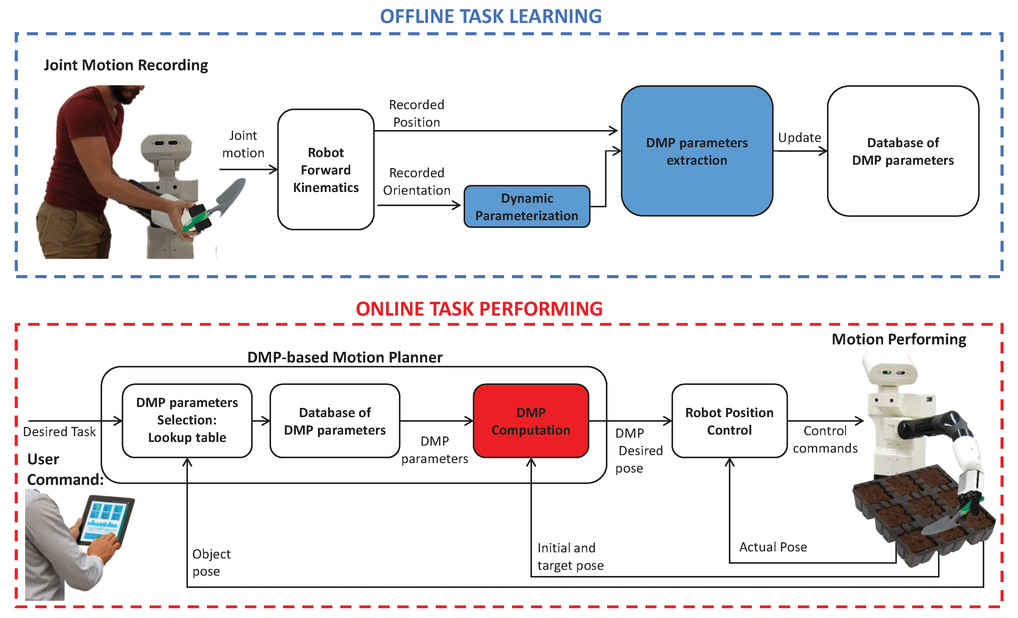
2.1. The Proposed DMP-Based Robot-Motion Planner with Dynamic Parameterization of the Orientation

A block scheme of the proposed DMP-based motion planner is shown in Figure 1. As for typical approaches, LbD based on DMPs consists of two phases. In the first phase, namely the offline task learning, trajectories executed by a demonstrator are recorded during the execution of a task, i.e., the human demonstrator manually moves the robotic arm by means of a hands-on approach and the position sensors embedded into the arm are used to record the joint motion. Hence, robot forward kinematics is adopted to retrieve the end-effector trajectory (position and orientation), and a dynamic parameterization method is used to avoid discontinuity in the orientation. Then, distinctive features (called DMP parameters) are subsequently extracted from these trajectories by using a Locally Weight Regression algorithm (LWR) in order to encode the robot motion (DMP parameters extraction).

In the second phase, i.e., the online task performing, depending on the task to be performed and on the target position to be reached, an online extraction of the DMP parameters from the dataset is performed by means of a lookup table method (DMP parameters selection), and DMPs are subsequently computed for each Cartesian DoF, as a sum of Gaussian kernels weighted by means of the previously computed DMP parameters (DMP computation). Finally, the computed DMPs are given as input for the robot position control, which provides the actuators commands to perform the desired task.

In Appendix A and Appendix B, theoretical details about DMPs and Lie groups are provided.

In the following, the new formulation of DMPs based on Lie theory and dynamic parameterization for the orientation is presented. In particular, the modules of DMP computation, DMP parameters extraction and dynamic parameterization for orientation are described.

2.1.1. DMP Computation for Orientation

A DMP formulation that could be extended to the orientation, expressed through either the rotation matrix or the unit Quaternion, is defined as

$$\tau \dot{\omega }={\alpha }_{\omega }\left({\beta }_{\omega }alog\left({\Phi }_t{\Phi }^{-1}\right)-\omega \right)+f_{\omega }$$

(1)

where $\tau$ is a time constant; ${\alpha }_{\omega }$ and ${\beta }_{\omega }$ are positive constants; ${\Phi }_t$ is the target orientation, expressed as rotation matrix or unit Quaternion; $\Phi$, $\omega$ and $\dot{\omega }$ are the orientation, angular velocity and angular acceleration, respectively; a is a parameter that is 1 if ${\Phi }_t$ and $\Phi$ are expressed as rotation matrices and 2 if they are expressed as unit Quaternions; and $f_{\omega }$ is the forcing term that implements the landscape attractor. It can be written as

$$f_{\omega }\left(x\right)=\frac{{\sum }_{i=1}^N{\mathsf{\Psi }}_i\left(x\right){\psi }_i}{{\sum }_{i=1}^N{\mathsf{\Psi }}_i\left(x\right)}xalog\left({\Phi }_t{\Phi }_0^{-1}\right)$$

(2)

where ${\Phi }_0$ is the end-effector initial orientation; x is the state variable of the system, defined in Equation (A4); and $log(.)$ is the logarithmic function that maps an element, $\Phi$, of the Lie group, e.g., $SO\left(3\right)$ or $S^3$, to an element belonging to the tangent space of that group, $\varphi$. The solution of Equation (1), i.e., $\Phi$, provides the orientation trajectory expressed by means of rotation matrices or unit Quaternions that can be found as

$$\Phi \left(t\right)=exp\left({\int }_{t_0}^t\omega \left(s\right)ds+\frac{1}{2}{\int \int }_{t_0}^t\dot{\omega }\left(s\right)d{s}^2\right)$$

(3)

where $t_0$ is the initial time and $exp(.)$ is the exponential function that maps an element of the tangent space, i.e., $\varphi$, to an element of the Lie group $SO\left(3\right)$ or $S^3$, i.e., $\Phi$.

2.1.2. DMP Parameters Extraction for Orientation

A locally weighted regression (LWR) algorithm [25] is adopted to learn DMP parameters $\Phi \left(t\right)$ in Equation (3).

Data on ${\Phi }_d$, ${\omega }_d$ and ${\dot{\omega }}_d$, i.e., the recorded orientation, angular velocity and angular acceleration, are inserted in the forcing term of Equation (2) as follows:

$$f_{\omega d}=\tau {\dot{\omega }}_d-{\alpha }_{\omega }\left({\beta }_{\omega }alog\left({\Phi }_t{\Phi }_d^{-1}\right)-{\omega }_d\right).$$

(4)

As for the position DMPs (see Appendix A), a function-approximation problem is formulated in order to find ${\psi }_i$ parameters that make $f_{\omega }$ as close as possible to $f_{\omega d}$. The cost function to be minimized is defined as

$$J_i=\sum _{t=1}^P{\mathsf{\Psi }}_i\left(t\right){\left(f_{\omega }\left(t\right)-{\psi }_i{ϵ}_{\omega }\left(t\right)\right)}^2$$

(5)

where

$${ϵ}_{\omega }\left(t\right)=xalog\left(\Phi {\Phi }_0^{-1}\right).$$

(6)

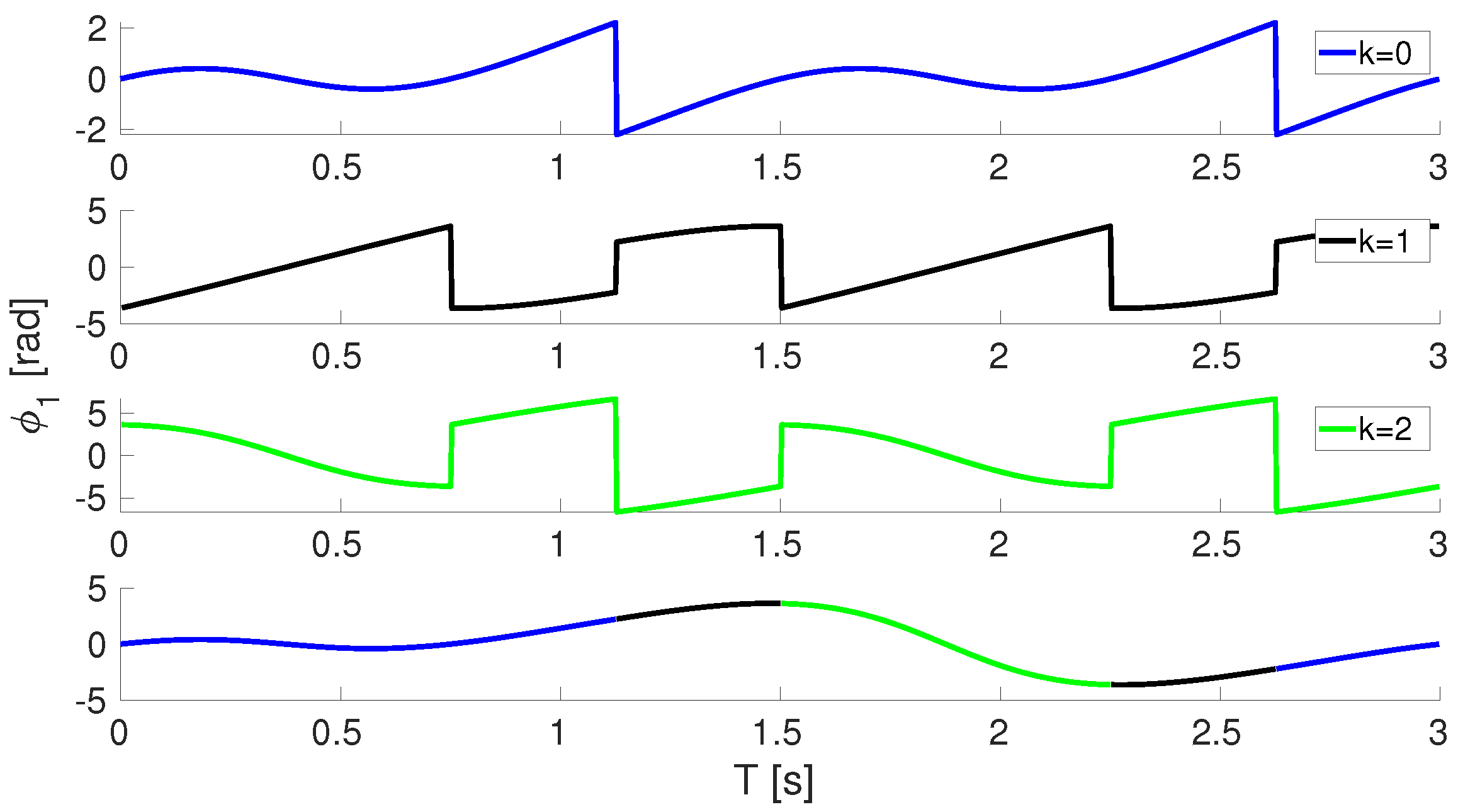
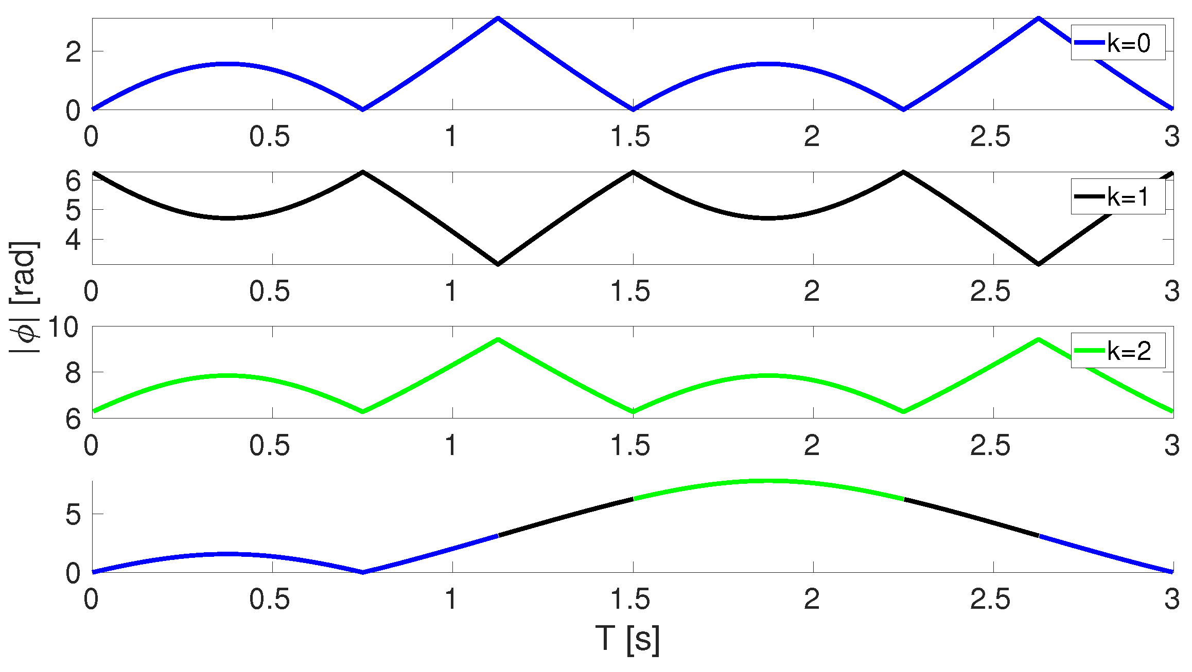
2.1.3. Dynamic Parameterization for Orientation

The main drawback of the DMP formulation based on Lie theory and proposed in Equations (1)–(4) is that the output of the logarithmic map has a gap of $2\pi$ when the norm of its argument is close to $\pi$. To the best of the authors’ knowledge, Learning by Demonstration approaches based on DMPs seem not to address this problem yet. Hence, in order to avoid discontinuity in the logarithmic map, a dynamic parameterization was introduced in Equations (1)–(4) as follows:

$$\tau \dot{\omega }={\alpha }_{\omega }\left({\beta }_{\omega }{v}_{k}alog\left({\Phi }_t{\Phi }^{-1}\right)-\omega \right)+f_{\omega }$$

(7)

where

$$f_{\omega d}=\tau {\dot{\omega }}_d-{\alpha }_{\omega }\left({\beta }_{\omega }{v}_{k}alog\left({\Phi }_t{\Phi }_d^{-1}\right)-{\omega }_d\right)$$

(8)

and

$$v_k=v_{k-1}\frac{1-2k\pi }{\parallel v_{k-1}\varphi \parallel }.k=1\dots n$$

(9)

In Equations (7)–(9), $\Phi \in {\mathbb{R}}^3$ is a 3 vector of coefficients such that $\omega =\frac{d\Phi }{dt}$. The rationale behind Equations (7)–(9) is explained in the following with a practical example.

Let us suppose the robot end effector is required to perform a rotation of $4\pi$ about the X, Y and Z axis, and let $R_{4\pi }$ be the rotation matrix that accounts for this rotation. The logarithmic map applied to $R_{4\pi }$, without dynamic parameterization ($k=0$), will give the solution $\Phi =[{\varphi }_1,{\varphi }_2,{\varphi }_2]$, whose first element ${\varphi }_1$ and norm $\parallel \Phi \parallel$ are shown in the blue line of Figure 2 and Figure 3. One can notice from these figures that ${\varphi }_1$ is discontinuous when $\parallel \Phi \parallel$ reaches $\pi$ or 0. For the sake of brevity, only ${\varphi }_1$ is reported, but the same discontinuities occur for ${\varphi }_2$ and ${\varphi }_3$.

Therefore, when LWR is adopted on these variables, the DMP parameters cannot be properly computed. Hence, the introduction of Equation (9) allows for the avoidance of this discontinuity by increasing or decreasing the k parameter when the discontinuity occurs. In Figure 2 and Figure 3, the output of the logarithmic map for different values of k is reported.

It is worth underlining that these parameterizations chosen for $\Phi$ account for the same rotation in $SO\left(3\right)$. In order to have a continuous function for $\Phi$, on which LWR could be properly adopted, different values for k in Equation (9) should be set. Simply, from Figure 2 and Figure 3, it is evident that when $\parallel \Phi \parallel$ reaches $(k+1)\pi$ and $\frac{d}{dt}\parallel \Phi \parallel >0$, the parameter k shall increase; conversely, when $\parallel \Phi \parallel$ reaches $k\pi$ and $\frac{d}{dt}\parallel \Phi \parallel <0$, the parameter k shall decrease. By doing this, one can obtain a continuous function of the element of $\Phi$, i.e., ${\varphi }_1$, ${\varphi }_2$ and ${\varphi }_3$, as shown in the multicolored line of Figure 2 and Figure 3.

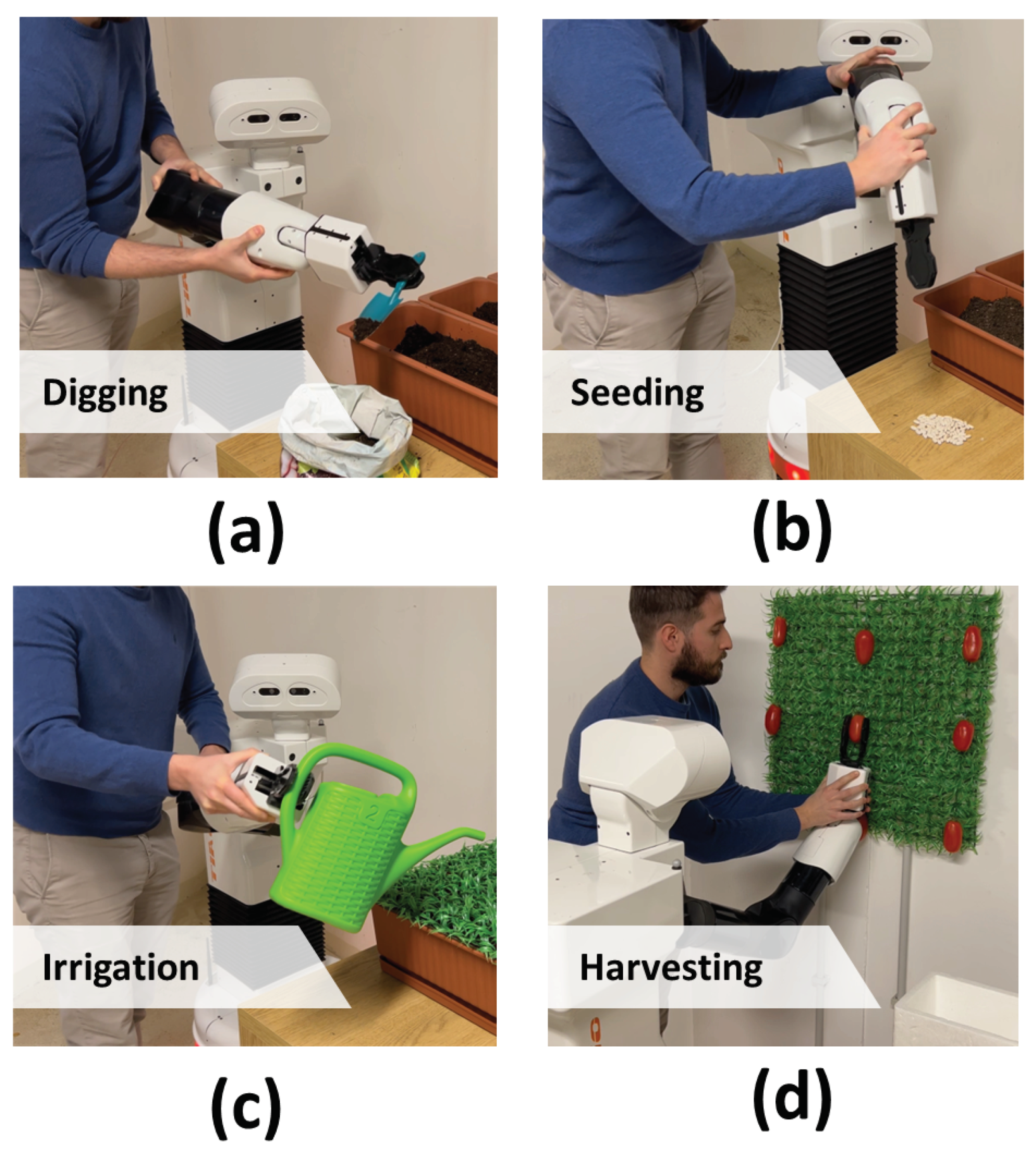
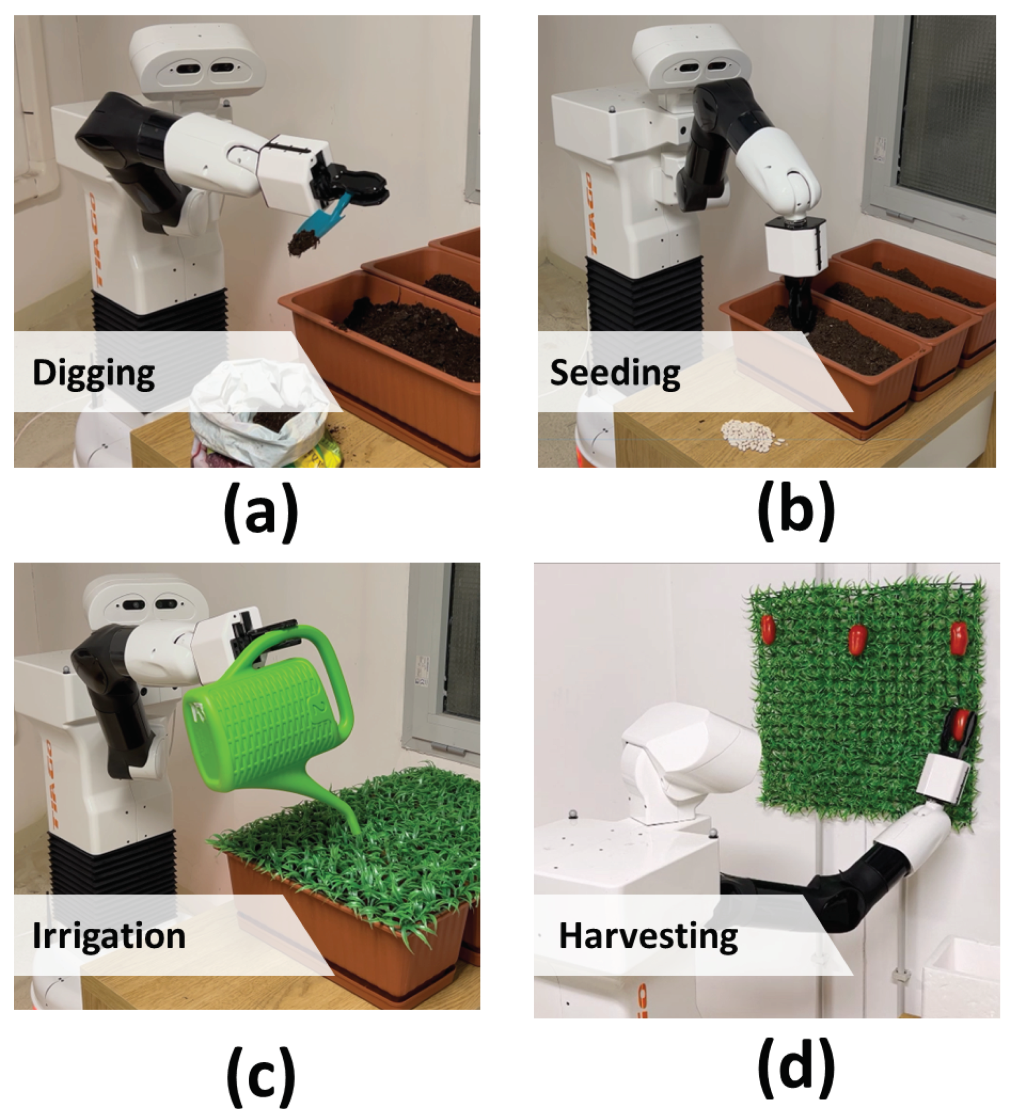
2.2. Application of the Proposed DMP-Based Motion Planner to Agricultural Robotics

Existing techniques of LbD are effectively used in many application fields to perform activities of daily living with robot aid. However, the adoption of DMPs for robot-motion planning in the agricultural domain is very limited [32,33]. In order to take a step forward with respect to the literature in this application domain and discuss the benefits of the proposed approach in terms of the reliability and effectiveness of the task execution, this section shows the experimental validation of the proposed DMP-based motion planner on agricultural activities. In the following, the (i) experimental robotic platform, (ii) experimental protocol and (iii) results and discussions are reported.

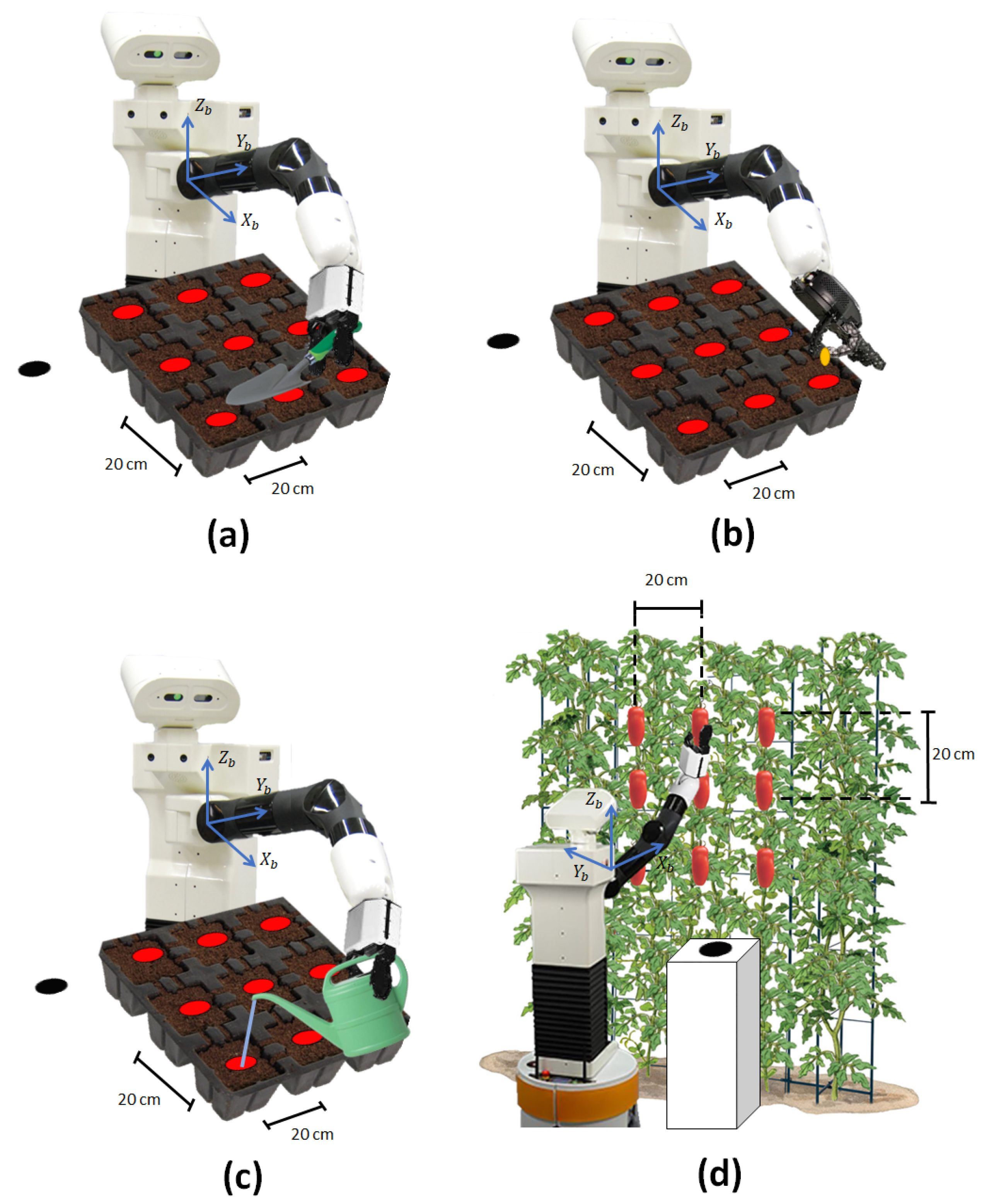
2.2.1. Experimental Robotic Platform

The proposed DMP-based motion planning was tested on the Tiago robot developed by Pal Robotics S.L. (Barcelona, Spain). The main robot components used to carry out the experimental validation are shown in Figure 1. They are (i) the RGB-D camera, (ii) the lifting torso, (iii) the 7 DoF arm and (iv) the Pal gripper. The RGB-D camera, i.e., the Astra S manufactured by Orbbec, is embedded in the Tiago’s head and is a short-range version of the Orbbec Astra Pro camera. It has a range of $[0.4;2]$ m. Tiago’s torso is the structure that supports the robot’s arm and head and is equipped with an internal lifter mechanism that allows the user to change the height of the robot. The lifter is able to move at 50 mm/s and has an RoM of 350 mm. The minimum and maximum height of the robot are $1.10$ m and $1.45$ m, respectively. Tiago’s arm is a 7 DoF anthropomorphic arm, composed of four M90 modules and one 3 DoF wrist. The Pal gripper contains two motors, each controlling one of the fingers. Each finger has a linear range of 4 cm.

2.2.2. Experimental Protocol

The experimental validation consisted of two phases, named the following: (a) offline task learning and (b) online task performing.

The 1st phase was aimed at recording the motion from a demonstrator during the execution of four working activities, i.e., digging, seeding, irrigation and harvesting, and to subsequently extract from this motion the set of DMP parameters to be stored in the database. Since there were no publicly available datasets for the specific activities to be carried out, an ad hoc database was built.

The 2nd phase was intended to validate the proposed approach and to assess its capacity to manage orientation discontinuity. For this purpose, the proposed approach grounded on Lie theory with dynamic parameterization, named proposed DMP planner, was compared to the one based on Euler angles, named conventional DMP planner based on Euler angles, and to the one based on Lie theory without dynamic parameterization, named conventional DMP planner based on Lie theory.

Offline Task Learning

In the 1st phase of the experimental validation, a human subject was asked to teach the robot how to perform the working activities, namely the digging, seeding, irrigation and harvesting, by means of a hands-on approach. In other words, the subject was required to passively move the robot arm in order to accomplish the task. During the task execution, the robot was piloted by means of a zero-torque control, and the sensors embedded in the robot, i.e., the encoders, were used to record the joints motion. The tasks are divided into several elementary actions (corresponding to the subtasks listed in

Table 1. Tasks description.

Task 1: Digging
Subtask 1-1	Tool reaching
Subtask 1-2	Digging
Subtask 1-3	Soil placing into the bucket
Subtask 1-4	Tool placing
Subtask 1-5	Homing
Task 2: Seeding
Subtask 2-1	Seed reaching
Subtask 2-2	Seed placing into the hall
Subtask 2-3	Homing
Task 3: Irrigation
Subtask 3-1	Reaching the watering can
Subtask 3-2	Irrigation
Subtask 3-3	Watering can placing
Subtask 3-4	Homing
Task 4: Harvesting
Subtask 4-1	Vegetable reaching
Subtask 4-2	Vegetable detaching from the plant
Subtask 4-3	Vegetable placing into the crate
Subtask 4-4	Homing

) and were performed for nine different positions of the targets. These positions are reported in Figure 4 for the four tasks.

Subsequently, Cartesian trajectories were computed by means of robot forward kinematics (FK) by adopting two different representations for the orientation, i.e., Euler angles (ZYZ) and unit Quaternion. Finally, a set of DMP parameters was computed for each object position by using Equations (A6) and (A7) for the position and Equations (5) and (6) for the orientation when the proposed DMP planner and the conventional DMP planner based on Lie theory were adopted. Conversely, Equations (A6) and (A7) were used for both the position and orientation when the conventional DMP planner based on Euler angles was adopted. In Figure 5 and Supplementary Materials, pictures and video of a human demonstrator teaching the robot how to perform digging, seeding, irrigation and harvesting tasks are shown.

Online Task Performing

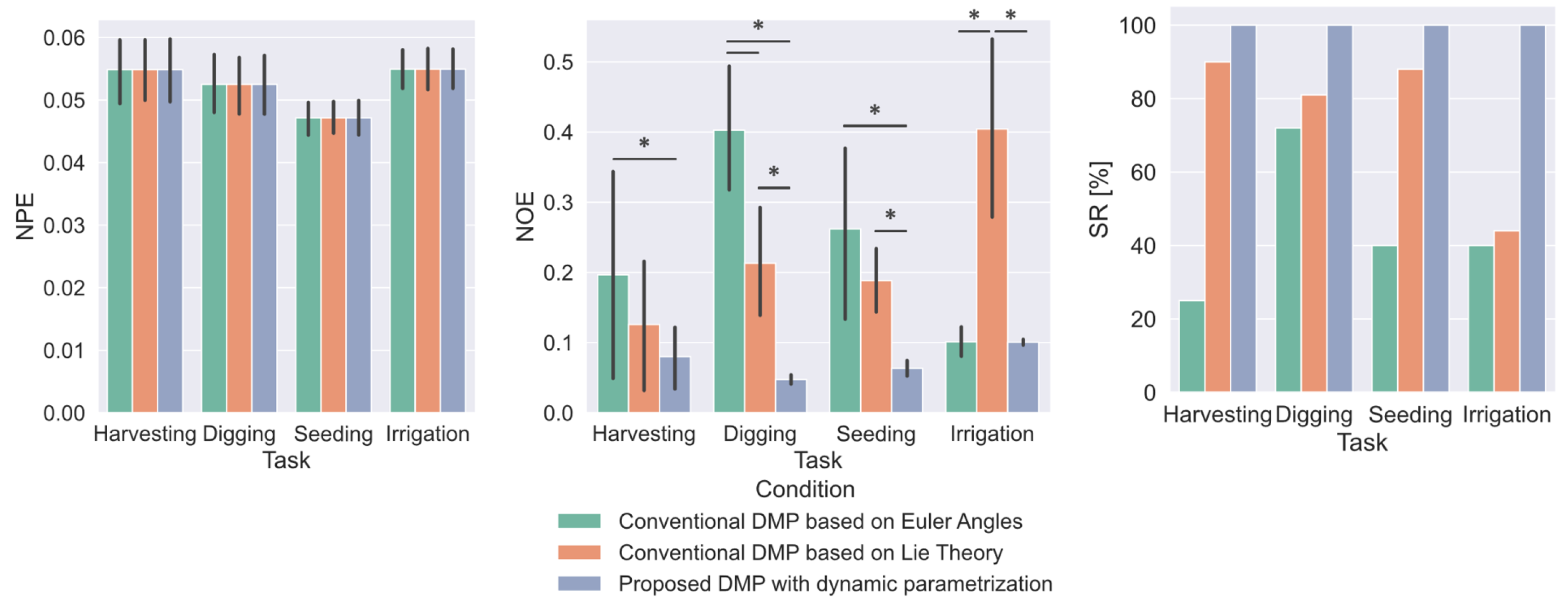
The 2nd phase of the experimental validation was aimed at assessing the capability of the proposed DMP planner to manage orientation discontinuity with respect to the conventional DMP planner based on Euler angles and to the conventional DMP planner based on Lie theory. DMPs were computed for each task and target position by using DMP parameters stored in the database. The robot arm was operated to perform the four tasks, i.e., digging, seeding, irrigation and harvesting, for the 9 different target positions shown in Figure 4 by using the three methods. In Figure 6 and Supplementary Materials, pictures and video of the robot while performing the learnt tasks, i.e., digging, seeding, irrigation and harvesting, are shown.

Performance Indices

Three performance indices, namely (i) the Normalized Position Error (NPE), (ii) the Normalized Orientation Error (NOE) and (iii) the success rate in managing orientation discontinuity (SR-MOD), were computed to perform the comparative analysis among the proposed DMP planner, the conventional DMP planner based on Euler angles and conventional DMP planner based on Lie theory.

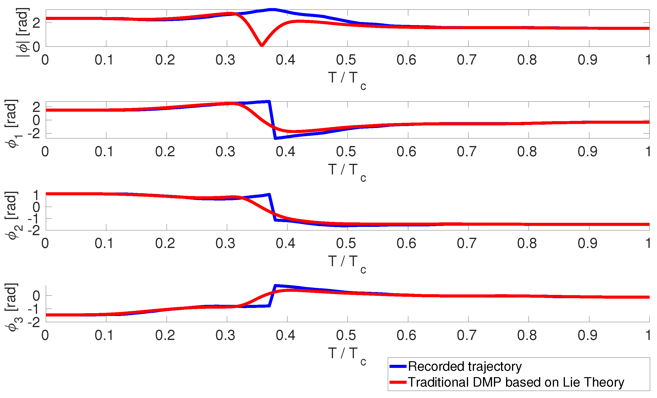
• The NPE and the NOE assess the capability of the proposed approach to accurately replicate the demonstrated motions. They are normalized with respect to the overall displacement of the recorded motion and are computed as follows:

  $$NPE=\frac{1}{N}·\frac{1}{\parallel g-y_0\parallel }\sum _{i=1}^N∥p\left(i\right)-p_m\left(i\right)∥$$

  (10)

  $$NOE=\frac{1}{N}·\frac{1}{∥log\left({\Phi }_0^{-1}{\Phi }_t\right)∥}\sum _{i=1}^N∥log\left(\Phi {\left(i\right)}^{-1}{\Phi }_m\left(i\right)\right)∥$$

  (11)

  where N is the number of collected samples; $p\left(i\right)$ and $\Phi \left(i\right)$ are the position and orientation expressed in unit Quaternion of the computed DMP, respectively; and $p_m\left(i\right)$ and ${\Phi }_m\left(i\right)$ are the recorded position and orientation at the i-th sample, respectively. The lower the NPE and NOE, the higher the trajectory reconstruction accuracy.
• The success rate in managing orientation discontinuity (SR-MOD) of the task execution is used to evaluate the capability of a given approach to accomplish the task and is evaluated as

  $$SR-MOD=\frac{N_{succ}}{N_{tot}}·100$$

  (12)

  where $N_{succ}$ is the number of trials successfully accomplished and $N_{tot}$ is the number of all the performed trials. A task is considered successfully accomplished if no singularity or discontinuity issues occur.

Statistical Analysis

The mean value and standard deviation (SD) of all the previously described indices were computed on multiple tasks (i.e., for 9 different target positions) for each DMP method. Each task was performed by the robot once. Since the data were not normally distributed, a statistical analysis based on a Wilcoxon paired-sample test was performed in order to carry out the comparative analysis among the different approaches, and a Bonferroni correction was applied on multiple comparisons (p-value $<0.05/N_c$, where $N_c$ is the number of comparisons).

3. Results and Discussions

The results of the comparative analysis among the three approaches are reported in Figure 7. The mean value and SD of the NPE and NOE were calculated on the nine target positions for each task and approach, i.e., the proposed DMP with dynamic parameterization, conventional DMP based on Euler angles and conventional DMP based on Lie theory.

As shown in Figure 7, the proposed approach outperforms the literature ones since it is able to better manage orientation-discontinuity issues compared to the two literature approaches (statically significant differences in terms of the NOE, i.e., with p-value $<0.01$, are highlighted by the star symbol in the figure).

Moreover, the results obtained by the three approaches in terms of the NPE are reported in Figure 7. They are the same for all the approaches since they differ from each other only in the formulation of the DMP orientation.

To stress the impact of the achieved results with respect to the considered application domain, i.e., the agricultural field, the SR-MOD of the task execution is also reported in Figure 7. This figure highlights that the complexity of the agricultural activities to be performed, which could require a high-orientation RoM to be performed, led very often to orientation discontinuities and, hence, to an unsuccessful execution of the task when the conventional DMP based on Euler angles and the conventional DMP based on Lie theory were adopted (some tasks, i.e., harvesting and seeding for the conventional DMP based on Euler angles and irrigation for the conventional DMP based on Lie theory, reported a very low SR-MOD $<40\%$). Hence, from these results, it emerges that the adoption of the proposed approach to planning complex activities in robotics, such as those to be performed in the agricultural domain, could significantly take a step forward with respect to the literature in terms of the reliability and effectiveness of the task execution.

Despite the proposed approach achieving a success rate of 100% for all the performed tasks, which means that it was always able to manage orientation discontinuities, no conclusion can be drawn about the performance of the overall system in difficult situations other than the ones tested in this work (for instance, picking vegetables hidden behind leaves, or moving the arm without colliding with surroundings and damaging crops). Indeed, the successful functioning of the robot in these scenarios may be impacted also by the performance of other modules included in the overall platform, e.g., the ability of the vision system to recognize and locate the fruits on the plants or the capability of the robotic arm to avoid obstacles in the scene [21].

In Figure 8 and Figure 9, two representative trajectories showing orientation-discontinuity issues are reported during the fulfillment of subtask 4-4. It is worth noticing from Figure 8 that when the argument of the logarithmic map, i.e., an element of the tangent space, has a norm close to $\pi$, the logarithmic map switches from positive to negative values, thus causing an incorrect computation of the DMP parameters. As well, the same error occurs in Figure 9 when the Pitch angle reaches $\pi$.

To give an idea of how the computed motion differs from the desired one when the three approaches are adopted, DMPs were computed on the orientation recorded during the fulfillment of subtask 4-4 and are reported in the same graphs. Figure 10 shows how the proposed DMP planner based on dynamic parameterization is able to overcome discontinuity in the logarithmic map and correctly compute DMPs differently from the conventional DMP based on Euler angles and the conventional DMP based on Lie theory.

Finally, for the sake of completeness, the proposed approach performance was also evaluated in terms of the system-response time, which is very critical for practical applications in real-world scenarios. Specifically, both the offline learning and online performing time were calculated. About the offline learning time, it is worth pointing out that the operator took 5 min, on average, to perform each demonstration with the robotic arm. Hence, considering that a total of nine trajectories were collected to build the entire database, the offline training phase lasted about 45 min, regardless of the specific representation used for the orientation. About the online performing time, the proposed DMP-based motion planner took $\left(2.57\pm 0.27\right)·{10}^{-3}$ s to generate the path of each subtask (a personal Computer Dell G5 15 5500 with Ubuntu 16.04 Operating System equipped with an Intel^® Core^™ i7-10870H processor at 8 × 5 GHz and 16 GB of RAM was used during the experiments). Moreover, the completion time needed to fulfill each subtask by the robot was a priori set to 10 s (this time could be varied on the basis of the user’s preferences).

4. Conclusions

In this work, a DMP-based robot-motion planner with dynamic parameterization of the orientation that could be effectively adopted for planning complex activities in robotics is proposed. The approach resorts to Lie theory and integrates into the DMP equations two important operations related to Lie algebra, namely the exponential and logarithmic map, which converts any element of the Lie group $SO\left(3\right)$ into an element of the tangent space $so\left(3\right)$ and vice versa. To manage orientation discontinuity, a dynamic parameterization for the element of the tangent space is shown in this work.

The impact of using such an LbD approach based on dynamic parameterization of the orientation to plan complex activities in the agricultural field was assessed; four agricultural activities, namely digging, seeding, irrigation and harvesting, were successfully taught to the Tiago robot, therefore taking a step forward with respect to the literature in this application domain.

The results obtained with the proposed approach demonstrated a high capability to manage orientation discontinuity (the mean NPE and NOE achieved by the proposed approach on average of the performed activities were $0.05\pm 0.01$ and $0.07\pm 0.11$, respectively); the success rate in managing orientation discontinuity was $100\%$ for all the tested target positions and activities and outperformed the ones obtained with the conventional methods based on the Euler angles and Lie theory, with an improvement in the SR-MOD of $55.75\%$ and $24.25\%$, respectively.

Moreover, from the achieved results, it emerged that the proposed method based on dynamic parameterization is inherently adoptable for tasks of different difficulty levels, as demonstrated in the experimental validation on different agricultural activities such as digging, seeding, irrigation and harvesting.

Future works will be mainly addressed to (i) increase the number of activities in the database, (ii) integrate into the framework an obstacle-avoidance module that enhances the robustness of the motion planner to external perturbations and (iii) assess the impact of using such an approach based on LbD with dynamic parameterization of the orientation on other application domains.

References

1. Maja, M.M.; Ayano, S.F. The impact of population growth on natural resources and farmers’ capacity to adapt to climate change in low-income countries. Earth Syst. Environ. 2021, 5, 271–283. [Google Scholar] [CrossRef]
2. Alexandra, R.; Péter, V.; Krisztina, D. Human resource aspect of agricultural economy–challenges of demographic change. APSTRACT Appl. Stud. Agribus. Commer. 2017, 11, 163–168. [Google Scholar]
3. Bac, C.W.; Van Henten, E.J.; Hemming, J.; Edan, Y. Harvesting robots for high-value crops: State-of-the-art review and challenges ahead. J. Field Robot. 2014, 31, 888–911. [Google Scholar] [CrossRef]
4. Adamides, G.; Edan, Y. Human–robot collaboration systems in agricultural tasks: A review and roadmap. Comput. Electron. Agric. 2023, 204, 107541. [Google Scholar] [CrossRef]
5. Duffy, B.R. Anthropomorphism and the social robot. Robot. Auton. Syst. 2003, 42, 177–190. [Google Scholar] [CrossRef]
6. Nguyen, T.T.; Kayacan, E.; De Baedemaeker, J.; Saeys, W. Task and motion planning for apple harvesting robot. IFAC Proc. Vol. 2013, 46, 247–252. [Google Scholar] [CrossRef]
7. Sucan, I.A.; Moll, M.; Kavraki, L.E. The open motion planning library. IEEE Robot. Autom. Mag. 2012, 19, 72–82. [Google Scholar] [CrossRef]
8. Jaulin, L. Path planning using intervals and graphs. Reliab. Comput. 2001, 7, 1–15. [Google Scholar] [CrossRef]
9. Jensen, M.A.F.; Bochtis, D.; Sørensen, C.G.; Blas, M.R.; Lykkegaard, K.L. In-field and inter-field path planning for agricultural transport units. Comput. Ind. Eng. 2012, 63, 1054–1061. [Google Scholar] [CrossRef]
10. Zeng, J.; Ju, R.; Qin, L.; Hu, Y.; Yin, Q.; Hu, C. Navigation in unknown dynamic environments based on deep reinforcement learning. Sensors 2019, 19, 3837. [Google Scholar] [CrossRef]
11. de Castro, G.G.; Berger, G.S.; Cantieri, A.; Teixeira, M.; Lima, J.; Pereira, A.I.; Pinto, M.F. Adaptive Path Planning for Fusing Rapidly Exploring Random Trees and Deep Reinforcement Learning in an Agriculture Dynamic Environment UAVs. Agriculture 2023, 13, 354. [Google Scholar] [CrossRef]
12. Fang, Z.; Liang, X. Intelligent obstacle avoidance path planning method for picking manipulator combined with artificial potential field method. Ind. Robot. Int. J. Robot. Res. Appl. 2022, 49, 835–850. [Google Scholar] [CrossRef]
13. Zhao, M.; Lv, X. Improved manipulator obstacle avoidance path planning based on potential field method. J. Robot. 2020, 2020, 1701943. [Google Scholar] [CrossRef]
14. Nguyen, T.T.; Kayacan, E.; De Baerdemaeker, J.; Saeys, W. Motion planning algorithm and its real-time implementation in apples harvesting robot. In Proceedings of the International Conference of Agricultural Engineering, Zurich, Switzerland, 6–10 July 2014. [Google Scholar]
15. Liu, C.; Feng, Q.; Tang, Z.; Wang, X.; Geng, J.; Xu, L. Motion Planning of the Citrus-Picking Manipulator Based on the TO-RRT Algorithm. Agriculture 2022, 12, 581. [Google Scholar] [CrossRef]
16. Chen, Y.; Fu, Y.; Zhang, B.; Fu, W.; Shen, C. Path planning of the fruit tree pruning manipulator based on improved RRT-Connect algorithm. Int. J. Agric. Biol. Eng. 2022, 15, 177–188. [Google Scholar] [CrossRef]
17. Argall, B.D.; Chernova, S.; Veloso, M.; Browning, B. A survey of robot learning from demonstration. Robot. Auton. Syst. 2009, 57, 469–483. [Google Scholar] [CrossRef]
18. Chen, J.R. Constructing task-level assembly strategies in robot programming by demonstration. Int. J. Robot. Res. 2005, 24, 1073–1085. [Google Scholar] [CrossRef]
19. Billard, A.; Calinon, S.; Dillmann, R.; Schaal, S. Handbook of robotics chapter 59: Robot programming by demonstration. In Handbook of Robotics; Springer: Berlin/Heidelberg, Germany, 2008. [Google Scholar]
20. Si, W.; Wang, N.; Yang, C. A review on manipulation skill acquisition through teleoperation-based learning from demonstration. Cogn. Comput. Syst. 2021, 3, 1–16. [Google Scholar] [CrossRef]
21. Lauretti, C.; Cordella, F.; Zollo, L. A hybrid joint/Cartesian DMP-based approach for obstacle avoidance of anthropomorphic assistive robots. Int. J. Soc. Robot. 2019, 11, 783–796. [Google Scholar] [CrossRef]
22. Ijspeert, A.J.; Nakanishi, J.; Hoffmann, H.; Pastor, P.; Schaal, S. Dynamical movement primitives: Learning attractor models for motor behaviors. Neural Comput. 2013, 25, 328–373. [Google Scholar] [CrossRef]
23. Lauretti, C.; Cordella, F.; Guglielmelli, E.; Zollo, L. Learning by Demonstration for planning activities of daily living in rehabilitation and assistive robotics. IEEE Robot. Autom. Lett. 2017, 2, 1375–1382. [Google Scholar] [CrossRef]
24. Saveriano, M.; Abu-Dakka, F.J.; Kramberger, A.; Peternel, L. Dynamic movement primitives in robotics: A tutorial survey. arXiv 2021, arXiv:2102.03861. [Google Scholar] [CrossRef]
25. Schaal, S.; Atkeson, C.G. Constructive incremental learning from only local information. Neural Comput. 1998, 10, 2047–2084. [Google Scholar] [CrossRef] [PubMed]
26. Tamantini, C.; Cordella, F.; Lauretti, C.; Zollo, L. The WGD—A Dataset of Assembly Line Working Gestures for Ergonomic Analysis and Work-Related Injuries Prevention. Sensors 2021, 21, 7600. [Google Scholar] [CrossRef] [PubMed]
27. Siciliano, B.; Sciavicco, L.; Villani, L.; Oriolo, G. Robotics–Modelling, Planning and Control; Advanced Textbooks in Control and Signal Processing Series; Springer: Berlin/Heidelberg, Germany, 2009. [Google Scholar]
28. Magermans, D.; Chadwick, E.; Veeger, H.; Van Der Helm, F. Requirements for upper extremity motions during activities of daily living. Clin. Biomech. 2005, 20, 591–599. [Google Scholar] [CrossRef] [PubMed]
29. Benos, L.; Tsaopoulos, D.; Bochtis, D. A review on ergonomics in agriculture. Part I: Manual operations. Appl. Sci. 2020, 10, 1905. [Google Scholar] [CrossRef]
30. Evans, D.J. On the representatation of orientation space. Mol. Phys. 1977, 34, 317–325. [Google Scholar] [CrossRef]
31. Ude, A.; Nemec, B.; Petrić, T.; Morimoto, J. Orientation in cartesian space dynamic movement primitives. In Proceedings of the 2014 IEEE International Conference on Robotics and Automation (ICRA), Hong Kong, China, 31 May–7 June 2014; pp. 2997–3004. [Google Scholar]
32. La Hera, P.; Morales, D.O.; Mendoza-Trejo, O. A study case of Dynamic Motion Primitives as a motion planning method to automate the work of forestry cranes. Comput. Electron. Agric. 2021, 183, 106037. [Google Scholar] [CrossRef]
33. Motokura, K.; Takahashi, M.; Ewerton, M.; Peters, J. Plucking motions for tea harvesting robots using probabilistic movement primitives. IEEE Robot. Autom. Lett. 2020, 5, 3275–3282. [Google Scholar] [CrossRef]
34. Chevalley, C. Theory of Lie Groups; Courier Dover Publications: Mineola, NY, USA, 2018. [Google Scholar]
Figure 1. Block scheme of the proposed DMP-based robot-motion planner with dynamic parameterization of the orientation.
Robotics 12 00166 g001
Figure 2. Parameterization of ϕ 1 for k = 0 , 1 , 2 .
Robotics 12 00166 g002
Figure 3. Parameterization of ϕ for k = 0 , 1 , 2 .
Robotics 12 00166 g003
Figure 4. A graphical illustration of the target positions for (a) digging, (b) seeding, (c) irrigation and (d) harvesting. In particular, the 9 tested target positions for subtasks 1-2, 2-2, 3-2 and 4-1 are shown in red. The first tested position (i.e., green point) with respect to the robot arm reference frame, i.e., [ X b , Y b , Z b ], is [ 20 ; 20 ; 40 ] cm for subtasks 1-2, 2-2 and 3-2. Conversely, for subtask 4-1, the first tested position is [ 50 ; 20 ; 0 ] cm. The target positions for subtasks 1-1, 1-3, 1-4, 2-1, 3-1, 3-3 and 4-3 are shown in black. The latter positions are always the same for the 9 repetitions of each task. It is worth pointing out that the tested scenario was structured in a way that no obstacles are on the collision course with the robot arm while reaching all the target positions.
Robotics 12 00166 g004
Figure 5. A picture of the offline task learning for (a) digging, (b) seeding, (c) irrigation and (d) harvesting. The robot is manually moved by a human demonstrator through a hands-on approach, and sensors embedded into the robotic arm are used to record the robot’s movements. Afterwards, DMP parameters are extracted from the recorded motion and stored in a database.
Robotics 12 00166 g005
Figure 6. A picture of the online task performance for (a) digging, (b) seeding, (c) irrigation and (d) harvesting. Parameters are selected from the database and used to compute DMPs with the 3 methods (i.e., the proposed DMP planner, the conventional DMP planner based on Euler angles and the conventional DMP planner based on Lie theory) for 9 different object positions.
Robotics 12 00166 g006
Figure 7. Experimental results obtained for the experimental session. Significantly different pairs of comparisons (p-value < 0.01) are denoted by a black line with a star symbol above.
Robotics 12 00166 g007
Figure 8. End-effector orientation during the fulfillment of subtask 4-4 (conventional Lie theory approach).
Robotics 12 00166 g008
Figure 9. End-effector orientation during the fulfillment of subtask 4-4 (Euler angles approach).
Robotics 12 00166 g009
Figure 10. End-effector orientation during the fulfillment of subtask 4-4 (proposed Lie theory approach with dynamic parameterization).
Robotics 12 00166 g010