Exponentially Correlated Hylleraas–Configuration Interaction Studies of Atomic Systems. III. Upper and Lower Bounds to He-Sequence Oscillator Strengths for the Resonance ¹S→¹P Transition

Abstract

The exponentially correlated Hylleraas–configuration interaction method (E-Hy-CI) is a generalization of the Hylleraas–configuration interaction method (Hy-CI) in which the single $r_{ij}$ of an Hy-CI wave function is generalized to a form of the generic type $r_{ij}^{{\nu }_{ij}}{e}^{-{\omega }_{ij}{r}_{ij}}$. This work continues the exploration, begun in the first two papers in this series (on the helium atom and on ground and excited $\mathrm{S}$ states of Li II), of whether wave functions containing both linear and exponential $r_{ij}$ factors converge more rapidly than either one alone. In the present study, we examined not only 1$s^2$ ${}^1\mathrm{S}$ states but 1s2p ${}^1\mathrm{P}$ states for the He I, Li II, Be III, C V and O VII members of the He isoelectronic sequence as well. All ${}^1\mathrm{P}$ energies except He I are better than previous results. The wave functions obtained were used to calculate oscillator strengths, including upper and lower bounds, for the He-sequence lowest (resonance) ${}^1\mathrm{S}\to$${}^1\mathrm{P}$ transition. Interpolation techniques were used to make a graphical study of the oscillator strength behavior along the isoelectronic sequence. Comparisons were made with previous experimental and theoretical results. The results of this study are oscillator strengths for the 1$s^2$ ${}^1\mathrm{S}\to$ 1s2$p{}^1\mathrm{P}$ He isoelectronic sequence with rigorous non-relativistic quantum mechanical upper and lower bounds of (0.001–0.003)% and probable precision ≤ 0.0000003, and were obtained by extending the previously developed E-Hy-CI formalism to include the calculation of transition moments (oscillator strengths).

1. Introduction

The Hylleraas–configuration interaction (Hy-CI) technique (developed by Sims and Hagstrom (SH) [1] and also independently by Woźnicki [2]) is a hybrid approach that attempts to combine the high precision of explicitly correlated traditional Hylleraas (Hy) [3] methods with the analytical tractability of strictly orbital-based configuration interaction (CI) methods [4]. The use of configurations wherever possible leads to less difficult integrals than in a purely Hy1 approach whose progress beyond the three electron atomic level has been hindered by the intractability of integrals involving nonseparable products of factors of the form $r_{12}{r}_{23}{r}_{34}$. If one restricts the wave function to at most a single, linear interelectronic distance $r_{ij}$ factor in each configuration state function (CSF), then the most difficult integrals are already dealt with at the four-electron level and the calculation retains the precision of Hy techniques, but is greatly simplified by the use of CI basis sets. However, for $N_e$ ≥ 4, there exists an ultimately slowly convergent “$r_{ij}{r}_{kl}$” double cusp that is built into Hy-CI for four or more electrons. Consequently, methods that speed up the convergence of an $r_{ij}$ factor can facilitate the extension of Hy-CI to systems with $N_e$ > 4.

In this paper, we continue to explore2 a generalization of the Hy-CI method proposed by Wang, Mei, Kurokawa, Nakashima and Nakatsuji [8], the exponentially correlated Hylleraas–configuration interaction (E-Hy-CI) method, in which the single $r_{ij}$ of an Hy-CI wave function is generalized to a form of the generic type $r_{ij}^{{\nu }_{ij}}{\mathrm{e}}^{-{\omega }_{ij}{r}_{ij}}$. Pairing an exponential $r_{ij}$ factor with linear $r_{ij}$ was first suggested for helium by Hirschfelder who, in 1960 [9], suggested that this type of correlation factor has the right behavior in the vicinity of the $r_{ij}$ cusp, and also has the right behavior as $r_{ij}$ goes to infinity. Whether functions having both linear and exponential $r_{ij}$ factors might be more rapidly convergent than either one alone was not demonstrated until our recent studies of the ground ${}^1$S state of the helium atom [6] and not only the ground 1 ${}^1\mathrm{S}$ state of the Li${}^{+}$ ion (Li II), but the 2 ${}^1\mathrm{S}$ through 6 ${}^1\mathrm{S}$ excited states as well [7].3 The present contribution continues this work by comparing the convergence of the E-Hy-CI wave function expansion to that of the Hy-CI wave function without exponential factors for states of non-$\mathrm{S}$ symmetry, specifically the 1s2$p{}^1\mathrm{P}$ (2 ${}^1\mathrm{P}$) state of some members of the He isoelectronic sequence.

The computed 1s2p ${}^1\mathrm{P}$ state wave functions were used with the previously obtained ${}^1\mathrm{S}$ wave functions (and some new ones for Li II, Be III, C V and O VII) to calculate He-sequence oscillator strengths, including upper and lower bounds, for the lowest ${}^1\mathrm{S}\to$${}^1\mathrm{P}$ transition.

The calculations reported in this work were obtained by solving the non-relativistic Schrödinger equation. Chung et al. [15] discussed the relative importance of correlation effects versus relativistic effects and stated that, for Z ≤ 27, correlation effects dominate relativistic effects. Consequently, one should start out with the best possible solutions to the non-relativistic Schrödinger equation and treat relativistic effects as a perturbation. Since this work considers first-row atoms for which Z ≤ 10, solving the non-relativistic Schrödinger equation is meaningful.

2. Variational Calculations

For $N_e$ electrons, the total non-relativistic, stationary-point-nucleus energy $E_{NR}$ is defined as the exact solution (eigenvalue) of the time-independent, non-relativistic Schrödinger equation

$$H_{NR}\Psi ({\mathbf{r}}_1,{\mathbf{r}}_2,...{\mathbf{r}}_{N_e})=E_{NR}\Psi ({\mathbf{r}}_1,{\mathbf{r}}_2,...{\mathbf{r}}_{N_e}),$$

(1)

where the Hamiltonian $H_{NR}$ is defined as (in hartree atomic units)

$$H_{NR}=\sum _{i=1}^{N_e}{\mathcal{H}}_i+\sum _{i<j}^{N_e}{r}_{ij}^{-1}.$$

(2)

Here, ${\mathcal{H}}_i$ = ${\mathcal{T}}_i+{\mathcal{V}}_i$, ${\mathcal{H}}_i$ being a one-electron operator (electron i) consisting of a kinetic energy part ${\mathcal{T}}_i=-\frac{1}{2}{\nabla }_i^2$ and a nuclear attraction part ${\mathcal{V}}_i=-Z/r_i$. $N_e$ denotes the number of electrons and Z the corresponding nuclear charge.

The E-Hy-CI wave function for $N_e$ electron atomic states is

$$\Psi =\sum _{K=1}^N{C}_K{\Phi }_K,$$

(3)

where

$${\Phi }_K=\Lambda \left(r_{ij}^{{\nu }_K}{\mathrm{e}}^{-{\omega }_K{r}_{ij}}\prod _{s=1}^{{\mathit{N}}_e}\left\{{\varphi }_{K_s}\left({\mathbf{r}}_{\mathbf{s}}\right)\right\}{\Theta }_K\right)={\mathit{O}}_{\mathit{as}}{\mathit{O}}_{\mathit{L},{\mathit{M}}_{\mathit{L}}}{\mathit{O}}_{\mathit{S},{\mathit{M}}_{\mathit{S}}}\left(r_{ij}^{{\nu }_K}{\mathrm{e}}^{-{\omega }_K{r}_{ij}}\prod _{s=1}^{{\mathit{N}}_e}\left\{{\varphi }_{K_s}\left({\mathbf{r}}_{\mathbf{s}}\right)\right\}{\Theta }_K\right)$$

(4)

denotes the $K$th antisymmetrized orbital and spin angular momentum projected explicitly correlated configuration state function (CSF). $\Lambda$ is the symmetry adaptation operator that performs the projection and is a product of an idempotent projection operator that makes the state antisymmetric, ${\mathit{O}}_{\mathit{as}}$, and ${\mathit{O}}_{\mathit{L},{\mathit{M}}_{\mathit{L}}}$, ${\mathit{O}}_{\mathit{S},{\mathit{M}}_{\mathit{S}}}$, the idempotent orbital and spin angular momentum projection operators of Löwdin type [16] for a state of total quantum numbers $L,M_L,S,M_S$ (Russell–Saunders ($LS$) coupling is assumed). Each term K contains at most one explicitly correlated factor $r_{ij}^{{\nu }_K}{\mathrm{e}}^{-{\omega }_K{r}_{ij}}$ that, in addition to the Hy-CI case with ${\omega }_K=0$, can also have ${\omega }_K\ne 0$. In practice, it is sufficient to take ${\nu }_K$ equal to 0 or 1, with ${\nu }_K=1$, ${\omega }_K=0$ the Hy-CI case and ${\nu }_K=0$, ${\omega }_K=0$ the CI case.4 ${\Theta }_K$ is a primitive spin product function for term K and ${\varphi }_{K_s}\left({\mathbf{r}}_{\mathbf{s}}\right)$ represents the sth basis orbital in the $K$th term.

The basis orbitals are un-normalized Slater-type orbitals (STOs) $\varphi \left(\mathbf{r}\right)$ that are defined as

$${\varphi }_i\left(\mathbf{r}\right)={[n_i,l_i,m_i]}_{{\xi }_i}^i=r^{n_i-1}{\mathrm{e}}^{-{\xi }_{i}r}{\mathit{Y}}_{l_i}^{m_i}(\theta ,\varphi ),$$

(5)

where $Y_l^m(\theta ,\varphi )$ is a normalized spherical harmonic in the Condon and Shortley phase convention [19]. With this choice of phase convention, the spherical harmonics satisfy

$$Y_l^{m\ast }(\theta ,\varphi )={(-1)}^m{Y}_l^{-m}(\theta ,\varphi ).$$

(6)

The coefficients $C_K$ in Equation (3) were found in this work by solving the generalized eigenvalue problem

$$\mathbf{HC}=E\mathbf{SC},$$

(7)

$$(\mathbf{H}-E_0\mathbf{S})\mathbf{C}=(E-E_0)\mathbf{SC},$$

(8)

$$\mathbf{C}=(E-E_0)(\mathbf{H}-E_0{\mathbf{S})}^{-\mathbf{1}}\mathbf{SC},$$

(9)

where the matrix elements are given by ${\mathcal{H}}_{KL}=\langle {\Phi }_K\left|\mathcal{H}\right|{\Phi }_L\rangle$ and ${\mathcal{S}}_{KL}=\langle {\Phi }_K|{\Phi }_L\rangle$ with the Hamiltonian H given by Equation (2) and $E_0$ being some starting approximation for the eigenvalue E of interest.

The details of how the authors solve this real symmetric-definite eigenvalue problem are discussed in [20], including how to obtain a quadruple precision version of our computationally fast Fortran 90+ portable parallel package suitable for large (80,000 × 80,000 or greater) dense matrices. All results reported in this article were obtained using real*32 extended precision (quad-double-with exponent or QDE, 256-bit, ≈64 digits) floating point arithmetic, and the message-passing interface (MPI) standard [21] was used to parallelize the code.

Method of Calculation

For two electrons, following Hy-CI [22], spin can be eliminated, and the E-Hy-CI wave function becomes [6,7]

$$\Psi ({\mathbf{r}}_1,{\mathbf{r}}_2)=\sum _{K=1}^N{C}_K{\Phi }_K({\mathbf{r}}_1,{\mathbf{r}}_2),$$

(10)

where the terms ${\Phi }_K$ are specifically of the form

$${\Phi }_K({\mathbf{r}}_1,{\mathbf{r}}_2)=(1\pm {\mathit{P}}_{\mathit{12}}){\mathit{O}}_{\mathit{L},{\mathit{M}}_{\mathit{L}}}\left(r_{12}^{{\nu }_K}{\mathrm{e}}^{-{\omega }_K{r}_{12}}{\varphi }_{K_1}\left({\mathbf{r}}_{\mathbf{1}}\right){\varphi }_{K_2}\left({\mathbf{r}}_{\mathbf{2}}\right)\right).$$

(11)

${\mathit{P}}_{\mathit{12}}$ is the operator that permutes electrons 1 and 2; the plus sign is for singlet levels and the minus sign is for triplet levels. Equation (2) becomes

$$H_{NR}={\mathcal{H}}_1+{\mathcal{H}}_2+{\mathcal{H}}_{12},$$

(12)

where ${\mathcal{H}}_{12}=r_{12}^{-1}$.

In the generalized eigenvalue problem $\mathbf{HC}=E\mathbf{SC}$, matrix element $H_{KL}$ is

$$H_{KL}=\langle {\Phi }_K\left|\mathcal{H}\right|{\Phi }_L\rangle =\langle \Lambda {\Phi }_K^P\left|\mathcal{H}\right|\Lambda {\Phi }_L^P\rangle ,$$

(13)

where ${\Phi }_K^P=r_{12}^{{\nu }_K}{\mathrm{e}}^{-{\omega }_K{r}_{12}}{\varphi }_{K_1}\left({\mathbf{r}}_{\mathbf{1}}\right){\varphi }_{K_2}\left({\mathbf{r}}_{\mathbf{2}}\right)$ denotes the $K$th primitive (unprojected) function as given in Equation (11) above. $S_{KL}$ is similar, with $\mathcal{H}$ replaced by the unit operator 1.

The projection reduction of these matrix elements is the same projection reduction used in Hy-CI calculations on lithium [23] and on beryllium [24] and is discussed in Appendix A of those references. The helium case is simpler so just the result is given here, which is that $H_{KL}$ is given by

$$\begin{array}{c}\hfill H_{KL}=\langle g_K{f}_K\left|\mathcal{H}\right|{\mathit{O}}_{\mathit{L},{\mathit{M}}_{\mathit{L}}}\mathit{B}\left({\mathit{g}}_{\mathit{L}}{\mathit{f}}_{\mathit{L}}\right)\rangle ,\end{array}$$

(14)

where $g_K\left(r_{12}\right)=r_{12}^{{\nu }_K}{\mathrm{e}}^{-{\omega }_K{r}_{12}}$ is the correlation factor and $f_K={\varphi }_{K_1}\left({\mathbf{r}}_{\mathbf{1}}\right){\varphi }_{K_2}\left({\mathbf{r}}_{\mathbf{2}}\right)$ is a product of un-normalized STOs (Equation (5)). In Equation (14), one can apply ${\mathit{O}}_{\mathit{L},{\mathit{M}}_{\mathit{L}}}$ either before or after applying B = 1 + ${\mathit{P}}_{\mathit{12}}$. The ${\mathit{O}}_{\mathit{L},{\mathit{M}}_{\mathit{L}}}$ projection is applied only on the orbital products since $g_L=r_{12}^{{\nu }_L}{\mathrm{e}}^{-{\omega }_L{r}_{12}}$ commutes with ${\mathit{O}}_{\mathit{L},{\mathit{M}}_{\mathit{L}}}$ [1].

In generalizing Hy-CI to E-Hy-CI for the two-electron He-sequence case, one merely has to take the correlation factor $g_K$ to be $g_K$ = $r_{12}^{{\nu }_K}{\mathrm{e}}^{-{\omega }_K{r}_{12}}$ in the formulas above since ${\mathrm{e}}^{-{\omega }_K{r}_{12}}$ has the same symmetry properties as $r_{12}$. Thus, $H_{KL}$ becomes

$$H_{KL}=\langle {\varphi }_{K_1}\left({\mathbf{r}}_1\right){\varphi }_{K_2}\left({\mathbf{r}}_2\right)r_{12}^{{\nu }_K}{\mathrm{e}}^{-{\omega }_K{r}_{12}}\left|\mathcal{H}\right|r_{12}^{{\nu }_L}{\mathrm{e}}^{-{\omega }_L{r}_{12}}(1+{\mathit{P}}_{\mathit{12}}){\mathit{O}}_{\mathit{L},{\mathit{M}}_{\mathit{L}}}\left({\varphi }_{L_1}\left({\mathbf{r}}_1\right){\varphi }_{L_2}\left({\mathbf{r}}_2\right)\right)\rangle .$$

(15)

A detailed discussion of the most general exponentially correlated integrals that have to be evaluated when using this wave function can be found in Section 3 of our recent study [6] of the ground state of helium.

3. Oscillator Strengths

The basic theory of electric dipole radiation in atomic systems was given by Condon and Shortley [19]; their terminology is followed closely herein. Assuming Russell–Saunders ($LS$) coupling and the non-relativistic many-electron Hamiltonian $H_{NR}$ (Equation (2)), the energy states of an atom are characterized by the set of quantum numbers $\gamma$$LS{M}_L{M}_S$ (here, $\gamma$ denotes the electronic configuration5). For an electric dipole transition connecting the terms (multiplets) $\gamma$$LS$ and ${\gamma }^{\prime }$$L^{\prime }{S}^{\prime }$, Condon and Shortley introduced the quantity $S($$\gamma$$LS$;${\gamma }^{\prime }{L}^{\prime }{S}^{\prime }$), called the absolute multiplet oscillator strength (line strength). It is defined in terms of the electric dipole moment operator

$$\overrightarrow{P}=\sum _{i=1}^{N_e}{\overrightarrow{r}}_i$$

(16)

by

$$S(\gamma LS;{\gamma }^{\prime }{L}^{\prime }{S}^{\prime })=\sum _{M_L,M_S}\sum _{M_L^{\prime },M_S^{\prime }}{|\langle \gamma LS{M}_L{M}_S\left|\overrightarrow{P}\right|{\gamma }^{\prime }{L}^{\prime }{S}^{\prime }{M}_L^{\prime }{M}_S^{\prime }\rangle |}^2.$$

(17)

The f-value or multiplet oscillator strength is related to S by

$$f(\gamma LS\to {\gamma }^{\prime }{L}^{\prime }{S}^{\prime })=\frac{2}{3}\frac{(E\left({\gamma }^{\prime }{L}^{\prime }{S}^{\prime }\right)-E\left(\gamma LS\right))}{(2L+1)(2S+1)}S(\gamma LS;{\gamma }^{\prime }{L}^{\prime }{S}^{\prime }).$$

(18)

The familiar electric dipole selection rules $\Delta S$ = 0, $\Delta$$M_S$ = 0, $\Delta L$ = $\pm 1$ and $\Delta$$M_L$ = 0, $\pm 1,$ hold for the Hamiltonian that we used. Moreover, given $\gamma LS$ and ${\gamma }^{\prime }$, $L^{\prime }(=L-1,L,L+1)$,$S^{\prime }$(=S), as a consequence of the Wigner–Eckart theorem, every nonvanishing matrix element of the operator $\overrightarrow{P}$ can be expressed in terms of a single parameter $\beta (\gamma LS;{\gamma }^{\prime }{L}^{\prime }{S}^{\prime })$ multiplied by expressions involving only $L,M_L$ and $M_L^{\prime }$. The parameter is independent of the quantum numbers $M_L,M_L^{\prime },M_S$ and $M_S^{\prime }$, the summation indices occurring in Equation (17). Consequently, the expressions for the multiplet oscillator strength may be written as products of a parameter $\beta (\gamma LS;{\gamma }^{\prime }{L}^{\prime }{S}^{\prime })$ and a single algebraic function of L and S resulting from the summation. Finally, notice that only one nonvanishing matrix element needs to be evaluated to determine a $\beta (\gamma LS;{\gamma }^{\prime }{L}^{\prime }{S}^{\prime })$, so, instead of computing all the matrix elements occurring in the summations in Equation (17), a single matrix element suffices to find the multiplet oscillator strength for a given $\gamma LS;{\gamma }^{\prime }{L}^{\prime }{S}^{\prime }$.

For the 1$s^2$ ${}^1\mathrm{S}\to$ 1s2$p{}^1\mathrm{P}$ transition, the ${}^1\mathrm{S}$ term consists of the one state with $L=M_L=0$, $S=M_S=0$. The 1s2$p{}^1\mathrm{P}$ term consists of three states corresponding to $S^{\prime }=M_S^{\prime }=0$, $L^{\prime }=1$ and $M_L^{\prime }=-1,0,1$. We choose to express ($\gamma$$LS$→${\gamma }^{\prime }$$L^{\prime }{S}^{\prime }$) in terms of the matrix element corresponding to the ${}^1\mathrm{P}$ state with $S^{\prime }=M_S^{\prime }=0$, $L^{\prime }=1$ and $M_L^{\prime }=0$. Then, Equation (17) for $L^{\prime }=L+1$ becomes (un-normalized wave functions), from Goldberg [25],

$$S(\gamma {}^1\mathrm{S};\gamma {}^{\prime }{}^1\mathrm{P})=3{\left|\frac{\langle \gamma {}^1\mathrm{S}\left|\overrightarrow{P}\right|\gamma {}^{\prime }{}^1\mathrm{P},M_{L^{\prime }}=0\rangle }{{\left[\langle \gamma {}^1\mathrm{S}|\gamma {}^1\mathrm{S}\rangle \langle \gamma {}^{\prime }{}^1\mathrm{P},M_{L^{\prime }}=0|\gamma {}^{\prime }{}^1\mathrm{P},M_{L^{\prime }}=0\rangle \right]}^{\frac{1}{2}}}\right|}^2$$

(19)

and we only need to construct $\gamma {}^1\mathrm{S}$ = $\Psi (1s^2$ ${}^1\mathrm{S}$) and $\gamma {}^{\prime }{}^1\mathrm{P}$ = $\Psi (1s2p$${}^1\mathrm{P}$) and evaluate Equation (19) to compute the line strength S and then the non-relativistic oscillator strength f.6

To evaluate Equation (19), we use the method developed by one of the authors (see Section 2.B in [29]) which leads to the following expression for S:

$$\begin{array}{c}\hfill S(\gamma {}^1\mathrm{S};\gamma {}^{\prime }{}^1\mathrm{P})=4\pi {\left|{\tilde{W}}_0\right|}^2=3{\tilde{W}}_{ab}^2,\end{array}$$

(20)

where $\left|{\tilde{W}}_0\right|$, the electronic dipole transition moment, is defined by

$$\begin{array}{cc}\hfill \left|{\tilde{W}}_0\right|& =\left|\langle \gamma {}^1\mathrm{S}\left|\sum _{i=1}^{N_e}{[2,1,0]}_0^i\right|\gamma {}^{\prime }{}^1\mathrm{P},M_{L^{\prime }}=0\rangle \right|\hfill \end{array}$$

(21)

in terms of un-normalized STOs (Equation (5)). To make the notation clearer, ${[2,1,0]}_0^i$ is just the STO $r_i{Y}_{l_i}^{m_i}({\theta }_i,{\varphi }_i)$, i.e., it is a $p_0$ STO whose orbital exponent equals 0.

To evaluate Equation (20), we use the fact that the wave functions employed to evaluate Equation (20) are given by Equations (3) and (4) and are linear combinations of antisymmetrized projected products of orbitals and at most one correlation factor of the form $r_{12}^{{\nu }_{12}}{e}^{-{\omega }_{12}{r}_{12}}$.

Thus,

$$\left|{\tilde{W}}_0\right|=\sum _{K,L}{C}_K{C}_L{\left|{\tilde{W}}_0\right|}_{KL},$$

(22)

where

$${\left|{\tilde{W}}_0\right|}_{KL}=\left|\langle {\Phi }_K\left|\sum _{i=1}^{N_e}{[2,1,0]}_0^i\right|{\Phi }_L\rangle \right|.$$

(23)

In Equation (23), ${\Phi }_L$ is a linear combination of orbitals and at most one correlation factor, so Equation (23) can be evaluated by expanding the product of ${[2,1,0]}_0^i$ and the appropriate STO of ${\Phi }_L$ in terms of STOs by the formulas given in a previous paper [30]. Then, the integrals required to evaluate Equation (20) are similar in type to those required to calculate overlap matrix elements using these wave functions and can be evaluated as described in the next section.

Transition Moment Integrals

In Equation (23), the exponentially correlated transition moment integrals that have to be evaluated are of the form

$$I_{\mathcal{R}}=\langle {\varphi }_1\left({\mathbf{r}}_1\right){\varphi }_2\left({\mathbf{r}}_2\right)r_{12}^{\nu }{\mathrm{e}}^{-\omega r_{12}}\left|\mathcal{R}\right|r_{12}^{{\nu }^{\prime }}{\mathrm{e}}^{-{\omega }^{\prime }{r}_{12}}{\varphi }_1^{\prime }\left({\mathbf{r}}_1\right){\varphi }_2^{\prime }\left({\mathbf{r}}_2\right)\rangle ,$$

(24)

where the operator $\mathcal{R}$ = ${[2,1,0]}_0^i$ for transition moment integrals. The key to evaluating these integrals is to recognize that we can convert these integrals into overlap integrals ($\mathcal{R}$ = 1) by recognizing that ${[2,1,0]}_0^i$ and ${\varphi }_i^{\prime }\left({\mathbf{r}}_i\right)$ are STOs and can be expanded in terms of STO-like functions $f_i\left(\mathbf{r}\right)$

$$f_i\left(\mathbf{r}\right)={[N_i,L_i,M_i]}_{{\omega }_i}=r^{N_i-1}{\mathrm{e}}^{-{\omega }_i{r}_i}{\mathit{Y}}_{L_i}^{M_i}(\theta ,\phi )$$

(25)

in a manner similar to the way “charge distributions” $\Omega \left(\mathbf{r}\right)$

$$\Omega \left(\mathbf{r}\right)={\varphi }^{\ast }\left(\mathbf{r}\right){\varphi }^{\prime }\left(\mathbf{r}\right)={[n,l,m]}_{\alpha }^{\ast }{[n^{\prime },l^{\prime },m^{\prime }]}_{{\alpha }^{\prime }}$$

(26)

are expanded. When ${\Omega }_i^{\prime }\left(\mathbf{r}\right)$ is given by

$${\Omega }^{\prime }\left(\mathbf{r}\right)=\varphi \left(\mathbf{r}\right){\varphi }^{\prime }\left(\mathbf{r}\right)={[n,l,m]}_{\alpha }{[n^{\prime },l^{\prime },m^{\prime }]}_{{\alpha }^{\prime }}$$

(27)

the formula becomes

$${\Omega }_i^{\prime }\left(\mathbf{r}\right)={(-1)}^{m_i}\sum _{L_i}{\left\{\frac{(2L_i+1)}{4\pi }\right\}}^{1/2}{c}^{L_i}\left(l_i^{\prime },m_i^{\prime };l_i,-m_i\right)f_i\left(\mathbf{r}\right),$$

(28)

where $N_i=n_i+n_i^{\prime }-1$ and the exponents are $w_i={\alpha }_i+{\alpha }_i^{\prime }$. $L_i$ satisfies the triangular inequality $|l_i-l_i^{\prime }|\le L_i\le l_i+l_i^{\prime }$, with $l_i+l_i^{\prime }+L_i=2g$ (g integral, i.e., the summation goes in steps of 2), and with the further restriction $L_i\ge \left|M_i\right|$, $M_i=m_i^{\prime }+m_i$. The $c^{L_i}$ are standard Condon and Shortley coefficients (the so-called $c^k$s) [19,30,31,32]. Using Equation (28) transforms the transition moment integrals into the form of Equation (19) of the first paper in this series [6] with $\mathcal{R}$ = 1, which can be evaluated by the methods of Section 3.1 of that paper.

4. Upper and Lower Bounds to Oscillator Strengths

The f-value or multiplet oscillator strength is notoriously sensitive to the wave functions employed in computing S via Equation (19) (S is then used in Equation (18) to compute f) [33,34] because significant contributions to the integral may arise from regions that do not significantly affect the energies of either state. To remedy this situation, Weinhold showed how to calculate rigorous upper and lower bounds to f-values (dipole oscillator strengths) from non-relativistic quantum mechanical principles [35,36]. While bounds were computed for a few atomic and molecular oscillator strengths [29,37,38,39], the rigorous bounds did not reflect the true precision of the computed oscillator strengths. For example, one of the co-authors calculated oscillator strengths, including rigorous (non-relativistic, infinite nuclear mass) quantum mechanical upper and lower bounds, for the lowest ${}^1\mathrm{S}$→${}^1\mathrm{P}$ transition of Be I, C III and O V [29] of (7–10)% and probable accuracy of ≤2%. The same co-author computed oscillator strengths, with rigorous upper and lower bounds, for the 16 lines arising from allowed transitions among the four lowest ${}^2\mathrm{S}$ and four lowest ${}^2\mathrm{P}$ states of Li I [38] of 3.5% in the best case ($1s^{2}2s{}^2\mathrm{S}\to 1s^{2}2p{}^2\mathrm{P}$) (the error in the best case was later shown to actually be approximately 0.3% [26]).

To obtain good bounds, the calculations have to be of higher precision, as was the case in the Anderson and Weinhold calculations of dipole oscillator strengths for He and Li${}^{+}$ in 1974 [37] in which a third of the calculated f-values were guaranteed to be 1% or better; in the best case (Li${}^{+}$ 2 ${}^3\mathrm{S}\to 2{}^3\mathrm{P}$), the bounds tightened to approximately 0.05%, around two orders of magnitude better than the corresponding experimental results. Perhaps because of the need for high precision, the most recent bounds calculation took place in 1976 (except for one in 1986 for the special case of the hydrogen atom [40] and one in 1988 for the special case of Hartree–Fock wave functions [41]). However, computational capacity has continued to evolve so that more and more high-precision wave functions are becoming available, and, in the case of the two-electron helium atom, the E-Hy-CI wave functions are precise enough energetically to suggest using them to compute oscillator strengths with upper and lower bounds to provide rigorous estimates of the uncertainty in the computed f-values.

Method of Calculation

Weinhold’s procedure [35] for calculating rigorous upper and lower bounds to dipole strengths actually computes bounds to the transition moment, from which, as we have seen, f-values (oscillator strengths) can be computed. In terms of approximate wave functions ${\psi }_a$ and ${\psi }_b$ for states a and b, respectively, the approximate transition moment is

$${\tilde{W}}_{ab}=\langle {\psi }_a\left|W_l\right|{\psi }_b\rangle .$$

(29)

The following additional quantities are required for the calculation of error bounds (see Section 2.C in [29]): the overlap integrals of the approximate wave functions ${\psi }_a,{\psi }_b$ with the true wave functions ${\Psi }_a,{\Psi }_b$,

$$S_a\equiv \langle {\psi }_a|{\Psi }_a\rangle ,S_b\equiv \langle {\psi }_b|{\Psi }_b\rangle ,$$

(30)

the corresponding overlap errors ${ϵ}_{a+}$, ${ϵ}_{b+}$,

$${ϵ}_{a+}\equiv {(1-S_{a-}^2)}^{\frac{1}{2}},{ϵ}_{b+}\equiv {(1-S_{b-}^2)}^{\frac{1}{2}},$$

(31)

and an uncertainty ${\Delta }_{ab}$ that is defined by

$${\Delta }_{ab}\equiv {(\langle {\psi }_b\left|W_l^2\right|{\psi }_b\rangle -{\tilde{W}}_{ab}^2)}^{1/2}.$$

(32)

Upper and lower bounds can then be calculated from the inequalities

$$\begin{array}{c}\hfill W_{ab}\lessgtr S_{a\pm }{S}_{b\pm }{\tilde{W}}_{ab}\pm {ϵ}_{a+}{S}_{b\pm }{\Delta }_{ab}\pm {ϵ}_{b+}{[{\langle {\Psi }_a\left|W_l^2\right|{\Psi }_a\rangle }_{+}-{(S_{a-}{\tilde{W}}_{ab}-{ϵ}_{a+}{\Delta }_{ab})}^2]}^{\frac{1}{2}},\end{array}$$

(33)

where the subscript ± signs mean the upper (+) or lower (-) bounds to the corresponding quantities.

With $|\tilde{W}|$’s defined by Equation (23), we have that

$$S(\gamma {}^1\mathrm{S};\gamma {}^{\prime }{}^1\mathrm{P})=4\pi {\left|{\tilde{W}}_0\right|}^2=3{\tilde{W}}_{ab}^2,$$

(34)

which relates upper and lower bounds to transition moments and upper and lower bounds to oscillator strengths.

5. ${}^1\mathrm{P}$ Wave Functions

The basis set orbitals in Hy-CI and E-Hy-CI atomic calculations are STOs; see Equation (5). For the nonlinear orbital exponent parameters for 1$s^2$ ${}^1\mathrm{S}$ (1 ${}^1\mathrm{S}$) states, the use of the “doubled” (orbital exponent) basis set E-Hy-CI introduced in paper I and continued in paper II was also continued here. In this treatment, the first set has an orbital with an orbital exponent $\xi$ that makes it essentially a valence shell orbital, whereas, for the second set, the orbital has a large exponent ${\xi }^{\prime }$ that brings it in closer to the nucleus. This approach is due to Drake [42,43], who pointed out the need for “doubling” basis sets so there is a natural partition of the basis set into two distinct distance scales: one appropriate for the complex correlated motion near the nucleus, and the other appropriate further out. The results are very good for the ground ${}^1\mathrm{S}$ state of helium [6] and Li${}^{+}$ ground and excited states [7] of ${}^1\mathrm{S}$ symmetry; that approach was continued here in the treatment of other members of the helium ${}^1\mathrm{S}$ isoelectronic sequence.

In contrast to the closed-shell 1$s^2$ ${}^1\mathrm{S}$ states, the ${}^1\mathrm{P}$ states are open-shell 1s2p ${}^1\mathrm{P}$ states with the two electrons having different symmetries. The two different orbital exponent basis sets for ${}^1\mathrm{P}$ are chosen to be representative of the two different electrons; there is no natural partition of the basis set into two distinct distance scales. In this case, pairing an exponential $r_{12}$ factor with linear $r_{12}$ may have an enhanced role in providing the right behavior in the vicinitiy of the $r_{12}$ cusp and also the right behavior as $r_{12}$ goes to infinity. How well this approach works for non-$\mathrm{S}$ states was studied by carrying out calculations on the lowest helium ${}^1\mathrm{P}$ state (2 ${}^1\mathrm{P}$) and then extending the He 2 ${}^1\mathrm{P}$ state calculation to other members of the He 2 ${}^1\mathrm{P}$ isoelectronic sequence.

It is worth noting that the ${}^1\mathrm{P}$ calculations are formally no different from the ${}^1\mathrm{S}$ calculations since the idempotent orbital and spin angular momentum projection operators of the Löwdin type in Equation (4) will project out linear combinations of the basis set orbitals with the correct orbital and spin angular momentum.

5.1. Comparison with Orthogonal Hy-CI

Table 1 presents a comparison of the convergence of an E-Hy-CI wave function expansion for He ${}^1\mathrm{P}$ with that of the Hy-CI wave function without exponential factors. Included also for comparison with these non-orthogonal wave function results are the orthogonal Hy-CI (O-Hy-CI) results of Zhang et al. [17]. The groundwork for O-Hy-CI was laid out in the 1960s by Szasz in his “General Theory of Correlated Wave Functions” [44], but his calculations were orthogonal Hy [45,46] (the orbitals were s-only STOs and not p-, d-, … orbitals, which are the hallmark of CI). The first genuine O-Hy-CI was carried out by Plute in 1984 [47] with calculations on four He states, the He ${}^1\mathrm{P}$ being the one relevant to this research. Using an s-, p-, d- and f- STO basis, Plute was able to achieve an energy of −2.1238 4260 hartree with 90 terms in the expansion, better at the time than all but the perimetric calculation of Schiff et al. [48] and the Hy calculation of Anderson and Weinhold [37]. To the authors’ knowledge, this remained the only O-Hy-CI calculation until the O-Hy-CI calculation of Zhang et al. [17], which is significant, as will be seen, in that the O-Hy-CI results, as do the E-Hy-CI results, speed up convergence over non-orthogonal Hy-CI wave functions and hence might help to overcome the ultimately slow convergence of “the $r_{ij}{r}_{kl}$ double cusp”, analogous to the $r_{ij}$ cusp problem for CI, that arises for $N_e$≥ four-electron systems.

5.2. Comparison of E-Hy-CI and Hy-CI

To clarify the E-Hy-CI and Hy-CI approach of the authors to orbital basis sets (and their optimization) for ${}^1\mathrm{P}$ states, consider Table 1. In contrast to ${}^1\mathrm{S}$ states, each line in the table specifies an inner set for the first electron and its associated l quantum number (=$l_{max}$), and an outer set with its associated and $l^{\prime }=l+1$ quantum number for the second electron. In the table, only the minimum information needed to specify the basis set is listed, namely an exponent $\xi$, the l quantum number for orbitals with that exponent, $n_{orbs}$, the number of orbitals with that exponent (the $n_i$ in Equation (5) run from $l_i+1$ to $l_i+n_{orbs}$), and ${\omega }_{12}$, the exponent of the exponentially correlated $r_{12}$ factor if this is an E-Hy-CI calculation. In all of the tables, N is used to refer to the number of terms in the wave function (see Equation (3)).

Table 1 displays the steps leading to the final 7744-term 2 ${}^1\mathrm{P}$ state wave function used in this work. Starting with a fixed ${\xi }^{\prime }$ = 1.085 for $l,l^{\prime }$ = {0,1}, $\xi$ was varied until the energy went through a minimum and there were enough data points to fit a smooth curve and yield an optimized $\xi$ = 2.272. Next, $\xi$ was fixed at 2.272 and ${\xi }^{\prime }$ was optimized in a similar fashion, yielding the optimized values of $\xi ,{\xi }^{\prime }$ = {2.272,1.291} for the $l,l^{\prime }=\{0,1\}$ 480 term wave function used in the optimization. $n_{orbs}$ and $n_{orbs}^{\prime }$ were then extended to 19 for an $l,l^{\prime }$ = {0,1} 722-term Hy-CI wave function of ≈0.015 millihartree precision. The effect of the exponential $r_{12}$ on the precision of the calculation is clearly evident when adding to each term an exponentially correlated ${\mathrm{e}}^{-{\omega }_{12}{r}_{12}}$ factor whose exponent ${\omega }_{12}$ is chosen to be the one (0.5) that satisfies the Kato cusp condition [49], yielding a 1444-term E-Hy-CI wave function of ≈15 $\mu$hartree precision. The speedup of O-Hy-CI over non-orthogonal Hy-CI wave functions is readily apparent at this point as the 514-term O-Hy-CI calculation of Zhang et al. [17] improves the 1444-term Hy-CI to greater than nanohartee precision (but the E-Hy-CI precision is better). This strategy was continued to the $l,l^{\prime }$ = {1,2} block, yielding optimized values of $\xi ,{\xi }^{\prime }$ = {1.955,2.25} for the 1444-term Hy-CI wave function and the 2888-term E-Hy-CI wave function, which is of ≈ picohartree precision. Thanks to the very high-precision exponentially correlated Hylleraas (E-Hy) calculation of Aznabaev et al. [50], it is clear that the $l_{max}$ = 3 (s-, p-, d- and f- STO) Hy-CI precision for this state is 10 decimal places and the E-Hy-CI precision is >13 decimal places, which is better than all previous calculations except for the Hy calculation of Drake [43] and the calculation by Aznabaev et al. The results from continuing the comparison through $l_{max}$ = 7 are tabulated in Table 1.

Table 1. Comparison of theoretical Hy-CI, E-Hy-CI and O-Hy-CI energies for the He 2 ${}^1\mathrm{P}$ state using two different orbital exponents ($\xi \ne {\xi }^{\prime }$) for electrons 1 and 2. Calculations utilized in obtaining the optimal $\xi$, ${\xi }^{\prime }$ are included. For each $l_{max}$, $l_{max}^{\prime }=l_{max}$ + 1. N is the number of terms in the expansion.

Technique	Author	${\mathit{l}}_{\mathit{max}}$	${\mathit{n}}_{\mathit{orbs}}$	$\mathit{\xi }$	${\mathit{l}}_{\mathit{max}}^{\prime }$	${\mathit{n}}_{\mathit{orbs}}^{\prime }$	${\mathit{\xi }}^{\prime }$	${\mathit{\omega }}_{12}$	N	Energy (Hartree)
Hy-CI 1	This work	0	16	2.28	1	15	1.085		480	−2.1238 2778 5160 1660 5130
Hy-CI	This work	0	16	2.272	1	15	1.085		480	−2.1238 2778 5160 4328 8615
Hy-CI	This work	0	16	2.270	1	15	1.085		480	−2.1238 2778 5160 4106 3517
Hy-CI	This work	0	16	2.272	1	15	1.300		480	−2.1238 2780 3592 4727 1690
Hy-CI	This work	0	16	2.272	1	15	1.291		480	−2.1238 2780 3657 1217 9787
Hy-CI	This work	0	16	2.272	1	15	1.290		480	−2.1238 2780 3655 3377 1118
Hy-CI	This work	0	16	2.272	1	15	1.291		480	−2.1238 2780 3657 1217 9787
E-Hy-CI	This work	0	16	2.272	1	15	1.291	0.5	960	−2.1238 4308 3927 0924 8309
Hy-CI	This work	0	19	2.272	1	19	1.291		722	−2.1238 2782 6872 0251 1341
E-Hy-CI	This work	0	19	2.272	1	19	1.291	0.5	1444	−2.1238 4308 5062 4897 8422
Hy-CI	This work	1	15	2.000	2	14	0.75		900	−2.1238 4303 4769 4360 5998
Hy-CI	This work	1	15	1.955	2	14	0.75		900	−2.1238 4303 4770 5696 3685
Hy-CI	This work	1	15	1.900	2	14	0.75		900	−2.1238 4303 4768 6097 2667
Hy-CI	This work	1	15	1.955	2	14	2.30		900	−2.1238 4307 3318 1068 7228
Hy-CI	This work	1	15	1.955	2	14	2.25		900	−2.1238 4307 3463 3468 4622
Hy-CI	This work	1	15	1.955	2	14	2.20		900	−2.1238 4307 2960 1221 3901
Hy-CI	This work	1	15	1.955	2	14	2.25		900	−2.1238 4307 3463 3468 4622
E-Hy-CI	This work	1	15	1.955	2	14	2.25	0.5	1800	−2.1238 4308 6441 2634 4197
Hy-CI	This work	1	19	1.955	2	19	2.25		1444	−2.1238 4307 5774 3704 6662
O-Hy-CI	Zhang et al. [17]	6 2		1.169 3	4 4		0.28419 3		514	−2.1238 4308 6457 05
E-Hy-CI	This work	1	19	1.955	2	19	2.25	0.5	2888	−2.1238 4308 6497 9644 7703
Hy-CI	This work	2	19	2.40	3	18	2.30		2128	−2.1238 4308 6479 8938 8807
E-Hy-CI	This work	2	19	2.40	3	18	2.30	0.5	4256	−2.1238 4308 6498 0912 9534
Hy-CI	This work	3	18	2.40	4	15	2.30		2668	−2.1238 4308 6491 8108 5041
E-Hy-CI	This work	3	18	2.40	4	15	2.30	0.5	5336	−2.1238 4308 6498 0989 3227
Hy-CI	This work	4	15	2.40	5	14	2.30		3088	−2.1238 4308 6491 9211 6091
E-Hy-CI	This work	4	15	2.40	5	14	2.30	0.5	6176	−2.1238 4308 6498 1004 0079
Hy-CI	This work	5	14	2.40	6	14	2.30		3480	−2.1238 4308 6491 9773 5726
E-Hy-CI	This work	5	14	2.40	6	14	2.30	0.5	6960	−2.1238 4308 6498 1008 1958
Hy-CI	This work	6	14	2.40	7	14	2.30		3872	−2.1238 4308 6492 0145 5741
E-Hy-CI	This work	6	14	2.40	7	14	2.30	0.5	7744	−2.1238 4308 6498 1009 6317
O-Hy-CI	Plute (1984) [47]								90	−2.1238 4260
Hy	AW 5 (1974) [37]			2.00			0.88		137	−2.1238 4303 14
Hy	SLPR 6 (1965) [48]								560	−2.1238 4308 5800
O-Hy-CI	Zhang et al. [17]	6 2		1.169 3	4 4		0.28419 3		514	−2.1238 4308 6457 05
Hy	Drake (1996) [43]								804	−2.1238 4308 6498 091
E-Hy-CI	This work	6	14	2.40	7	14	2.30	0.5	7744	−2.1238 4308 6498 1009 6317
Reference	Aznabaev et al. [50]								22,000	−2.1238 4308 6498 1013 5924
(E-Hy) 7	(2018)									… 7333 1423 74

Note: All energies in this work are variational; all calculations were carried out in quadruple-double-with exponent (QDE) precision. ¹ For a detailed discussion of both E-Hy-CI and Hy-CI, including how they compare with the other methods in this table and elsewhere in this research, see the authors’ review article [14]. ² 6 here represents $n_{orbs}$ = 7, 6, 5, 4, 3, 2 and 1, respectively, for $l=0-6$. ³ Jiao [51]. ⁴ 4 here represents $n_{orbs}^{\prime }$ = 5, 4, 3, 2 and 1, respectively, for $l^{\prime }=0-4$. ⁵ Anderson and Weinhold. ⁶ Schiff, Lifson, Pekeris and Rabinowitz. ⁷ This line continues the line above, giving the trailing digits from Table II of Aznabaev et al. [50].

Table 1. Comparison of theoretical Hy-CI, E-Hy-CI and O-Hy-CI energies for the He 2 ${}^1\mathrm{P}$ state using two different orbital exponents ($\xi \ne {\xi }^{\prime }$) for electrons 1 and 2. Calculations utilized in obtaining the optimal $\xi$, ${\xi }^{\prime }$ are included. For each $l_{max}$, $l_{max}^{\prime }=l_{max}$ + 1. N is the number of terms in the expansion.

Technique	Author	${\mathit{l}}_{\mathit{max}}$	${\mathit{n}}_{\mathit{orbs}}$	$\mathit{\xi }$	${\mathit{l}}_{\mathit{max}}^{\prime }$	${\mathit{n}}_{\mathit{orbs}}^{\prime }$	${\mathit{\xi }}^{\prime }$	${\mathit{\omega }}_{12}$	N	Energy (Hartree)
Hy-CI 1	This work	0	16	2.28	1	15	1.085		480	−2.1238 2778 5160 1660 5130
Hy-CI	This work	0	16	2.272	1	15	1.085		480	−2.1238 2778 5160 4328 8615
Hy-CI	This work	0	16	2.270	1	15	1.085		480	−2.1238 2778 5160 4106 3517
Hy-CI	This work	0	16	2.272	1	15	1.300		480	−2.1238 2780 3592 4727 1690
Hy-CI	This work	0	16	2.272	1	15	1.291		480	−2.1238 2780 3657 1217 9787
Hy-CI	This work	0	16	2.272	1	15	1.290		480	−2.1238 2780 3655 3377 1118
Hy-CI	This work	0	16	2.272	1	15	1.291		480	−2.1238 2780 3657 1217 9787
E-Hy-CI	This work	0	16	2.272	1	15	1.291	0.5	960	−2.1238 4308 3927 0924 8309
Hy-CI	This work	0	19	2.272	1	19	1.291		722	−2.1238 2782 6872 0251 1341
E-Hy-CI	This work	0	19	2.272	1	19	1.291	0.5	1444	−2.1238 4308 5062 4897 8422
Hy-CI	This work	1	15	2.000	2	14	0.75		900	−2.1238 4303 4769 4360 5998
Hy-CI	This work	1	15	1.955	2	14	0.75		900	−2.1238 4303 4770 5696 3685
Hy-CI	This work	1	15	1.900	2	14	0.75		900	−2.1238 4303 4768 6097 2667
Hy-CI	This work	1	15	1.955	2	14	2.30		900	−2.1238 4307 3318 1068 7228
Hy-CI	This work	1	15	1.955	2	14	2.25		900	−2.1238 4307 3463 3468 4622
Hy-CI	This work	1	15	1.955	2	14	2.20		900	−2.1238 4307 2960 1221 3901
Hy-CI	This work	1	15	1.955	2	14	2.25		900	−2.1238 4307 3463 3468 4622
E-Hy-CI	This work	1	15	1.955	2	14	2.25	0.5	1800	−2.1238 4308 6441 2634 4197
Hy-CI	This work	1	19	1.955	2	19	2.25		1444	−2.1238 4307 5774 3704 6662
O-Hy-CI	Zhang et al. [17]	6 2		1.169 3	4 4		0.28419 3		514	−2.1238 4308 6457 05
E-Hy-CI	This work	1	19	1.955	2	19	2.25	0.5	2888	−2.1238 4308 6497 9644 7703
Hy-CI	This work	2	19	2.40	3	18	2.30		2128	−2.1238 4308 6479 8938 8807
E-Hy-CI	This work	2	19	2.40	3	18	2.30	0.5	4256	−2.1238 4308 6498 0912 9534
Hy-CI	This work	3	18	2.40	4	15	2.30		2668	−2.1238 4308 6491 8108 5041
E-Hy-CI	This work	3	18	2.40	4	15	2.30	0.5	5336	−2.1238 4308 6498 0989 3227
Hy-CI	This work	4	15	2.40	5	14	2.30		3088	−2.1238 4308 6491 9211 6091
E-Hy-CI	This work	4	15	2.40	5	14	2.30	0.5	6176	−2.1238 4308 6498 1004 0079
Hy-CI	This work	5	14	2.40	6	14	2.30		3480	−2.1238 4308 6491 9773 5726
E-Hy-CI	This work	5	14	2.40	6	14	2.30	0.5	6960	−2.1238 4308 6498 1008 1958
Hy-CI	This work	6	14	2.40	7	14	2.30		3872	−2.1238 4308 6492 0145 5741
E-Hy-CI	This work	6	14	2.40	7	14	2.30	0.5	7744	−2.1238 4308 6498 1009 6317
O-Hy-CI	Plute (1984) [47]								90	−2.1238 4260
Hy	AW 5 (1974) [37]			2.00			0.88		137	−2.1238 4303 14
Hy	SLPR 6 (1965) [48]								560	−2.1238 4308 5800
O-Hy-CI	Zhang et al. [17]	6 2		1.169 3	4 4		0.28419 3		514	−2.1238 4308 6457 05
Hy	Drake (1996) [43]								804	−2.1238 4308 6498 091
E-Hy-CI	This work	6	14	2.40	7	14	2.30	0.5	7744	−2.1238 4308 6498 1009 6317
Reference	Aznabaev et al. [50]								22,000	−2.1238 4308 6498 1013 5924
(E-Hy) 7	(2018)									… 7333 1423 74

Note: All energies in this work are variational; all calculations were carried out in quadruple-double-with exponent (QDE) precision. ¹ For a detailed discussion of both E-Hy-CI and Hy-CI, including how they compare with the other methods in this table and elsewhere in this research, see the authors’ review article [14]. ² 6 here represents $n_{orbs}$ = 7, 6, 5, 4, 3, 2 and 1, respectively, for $l=0-6$. ³ Jiao [51]. ⁴ 4 here represents $n_{orbs}^{\prime }$ = 5, 4, 3, 2 and 1, respectively, for $l^{\prime }=0-4$. ⁵ Anderson and Weinhold. ⁶ Schiff, Lifson, Pekeris and Rabinowitz. ⁷ This line continues the line above, giving the trailing digits from Table II of Aznabaev et al. [50].

The formula of Pekeris and co-workers [48],

$$E_{extrapolated}=E_1+\frac{(E_1-E_0)(E_2-E_1)}{2E_1-E_0-E_2},$$

(35)

where the $E_0$, $E_1$ and $E_2$ values are the 6176, 6960 and 7744-term results in Table 1, is used to extrapolate to an estimated exact non-relativistic energy of this state.

These Table 1 results show dramatic improvements:

• Hy-CI $sp$-wave 4 decimal place precision becomes 8 decimal place E-Hy-CI $sp$-wave precision (> Hy-CI $pd$-wave precision),
• Hy-CI $pd$-wave 7 decimal place precision becomes 11 decimal place E-Hy-CI $pd$-wave precision (> Hy-CI l = 7 precision),
• already at the E-Hy-CI $pd$-wave expansion, the result is better than the Hy-CI l = 7 result.

It is clear from the Table 1 results that the 14 decimal place l = 7 Hy-CI result can be improved on with just an l = 3 E-Hy-CI basis; this demonstrates that the E-Hy-CI speed-up convergence over non-orthogonal Hy-CI wave functions for $\mathrm{S}$ states continues for non-$\mathrm{S}$ states as well (specifically, for $\mathrm{P}$ states).

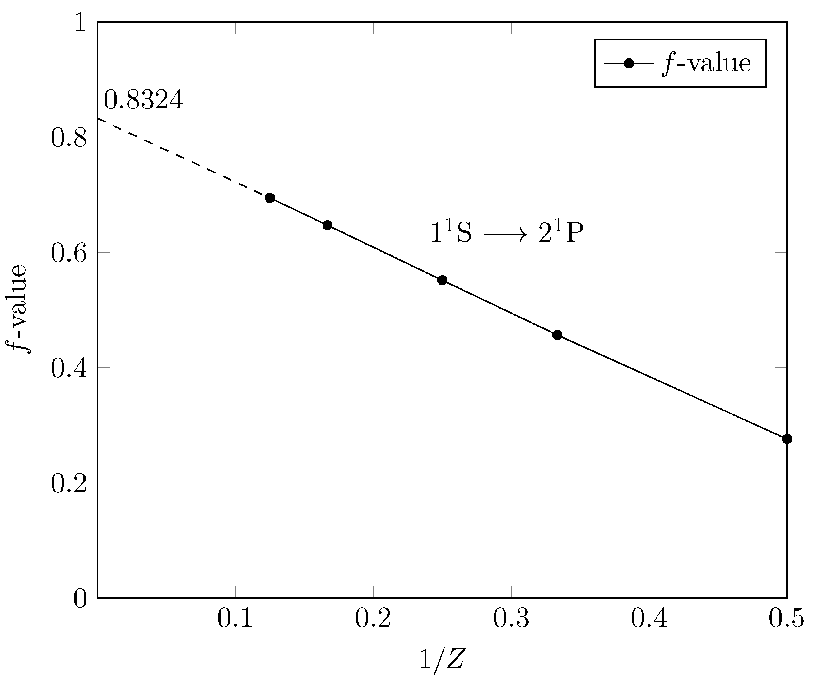
6. Isoelectronic Sequences

The 8568-term wave function for the 1$s^2$ ${}^1\mathrm{S}$ state of He I of estimated 20 decimal digit precision and the 7744-term wave function for the 1s2p ${}^1\mathrm{P}$ state of estimated 16 decimal digit precision were used to calculate wave functions and energies for other members of the He isoelectronic sequence, namely Li II, Be III, C V and O VII. For these results, no exponent minimization was performed, just a simple nuclear charge-based scaling of the wave functions of Table 4 of Sims et al. [6] and Table 1, respectively. For example, the results for Be III were obtained by scaling the orbital exponents by a factor of 4.0/2.0 and, for C V, the orbital exponents were scaled by a factor of 6.0/2.0. Our results are tabulated in

Table 2. Correlated wave function He isoelectronic sequence 1 ${}^1\mathrm{S}$ and 2 ${}^1\mathrm{P}$ non-relativistic energies. N is the number of terms in the expansion.

State	Technique	Author	N	Energy (Hartree)
He 1 ${}^1\mathrm{S}$	E-Hy-CI	Sims et al. (2020) [6]	8568	−2.9037 2437 7034 1195 9830 94
He 1 ${}^1\mathrm{S}$	ICI	Nakashima and Nakatsuji (2008) [52]	22,709	−2.9037 2437 7034 1195 9831 12
Li II 1 ${}^1\mathrm{S}$	E-Hy-CI	Sims et al. (2021) [7]	8568	−7.2799 1341 2669 3059 6491 66
Li II 1 ${}^1\mathrm{S}$	ICI	Nakashima and Nakatsuji (2008) [52]	22,709	−7.2799 1341 2669 3059 6491 95
Be III 1 ${}^1\mathrm{S}$	E-Hy-CI	This work	8568	−13.6555 6623 8423 5867 0207 77
Be III 1 ${}^1\mathrm{S}$	ICI	Nakashima and Nakatsuji (2008) [52]	9682	−13.6555 6623 8423 5867 0208 17
C V 1 ${}^1\mathrm{S}$	E-Hy-CI	This work	8568	−32.4062 4660 1898 5303 1055 17
C V 1 ${}^1\mathrm{S}$	ICI	Nakashima and Nakatsuji (2008) [52]	9682	−32.4062 4660 1898 5303 1055 74
O VII 1 ${}^1\mathrm{S}$	E-Hy-CI	This work	8568	−59.1565 9512 2757 9255 5854 43
O VII 1 ${}^1\mathrm{S}$	ICI	Nakashima and Nakatsuji (2008) [52]	9682	−59.1565 9512 2757 9255 5854 99
He 2 ${}^1\mathrm{P}$	E-Hy-CI	This work	6176	−2.1238 4308 6498 1004 0079
He 2 ${}^1\mathrm{P}$	E-Hy-CI	This work	6960	−2.1238 4308 6498 1008 1958
He 2 ${}^1\mathrm{P}$	E-Hy-CI	This work	7744	−2.1238 4308 6498 1009 6317
He 2 ${}^1\mathrm{P}$	Extrapolated	This work		−2.1238 4308 6498 1010(3)
He 2 ${}^1\mathrm{P}$	E-Hy	Aznabaev et al. (2018) [50]	22,000	−2.1238 4308 6498 1013 5925
Li II 2 ${}^1\mathrm{P}$	E-Hy-CI	This work	6176	−4.9933 5107 7780 0153 5568
Li II 2 ${}^1\mathrm{P}$	E-Hy-CI	This work	6960	−4.9933 5107 7780 0155 3584
Li II 2 ${}^1\mathrm{P}$	E-Hy-CI	This work	7744	−4.9933 5107 7780 0159 3316
Li II 2 ${}^1\mathrm{P}$	Extrapolated	This work		−4.9933 5107 7780 0165(3)
Li II 2 ${}^1\mathrm{P}$	ECS 1	Cann and Thakkar (1992) [53]	100	−4.9933 5107 21
Be III 2 ${}^1\mathrm{P}$	E-Hy-CI	This work	6176	−9.1107 7162 2916 4383 9458
Be III 2 ${}^1\mathrm{P}$	E-Hy-CI	This work	6960	−9.1107 7162 2916 4397 2592
Be III 2 ${}^1\mathrm{P}$	E-Hy-CI	This work	7744	−9.1107 7162 2916 4406 7410
Be III 2 ${}^1\mathrm{P}$	Extrapolated	This work		−9.1107 7162 2916 442(2)
Be III 2 ${}^1\mathrm{P}$	ECS	Cann and Thakkar (1992) [53]	100	−9.1107 7161 42
C V 2 ${}^1\mathrm{P}$	E-Hy-CI	This work	6176	−21.0933 3231 3388 3968 4013
C V 2 ${}^1\mathrm{P}$	E-Hy-CI	This work	6960	−21.0933 3231 3388 3993 9969
C V 2 ${}^1\mathrm{P}$	E-Hy-CI	This work	7744	−21.0933 3231 3388 4009 9911
C V 2 ${}^1\mathrm{P}$	Extrapolated	This work		−21.0933 3231 3388 403(2)
C V 2 ${}^1\mathrm{P}$	ECS	Cann and Thakkar (1992) [53]	100	−21.0933 3230 09
O VII 2 ${}^1\mathrm{P}$	E-Hy-CI	This work (QP)	7744	−38.0747 3523 5875 4074
O VII 2 ${}^1\mathrm{P}$	E-Hy-CI	This work	6176	−38.0747 3523 5875 4922 2755
O VII 2 ${}^1\mathrm{P}$	E-Hy-CI	This work	6960	−38.0747 3523 5875 5174 8235
O VII 2 ${}^1\mathrm{P}$	E-Hy-CI	This work	7744	−38.0747 3523 5875 5321 5034
O VII 2 ${}^1\mathrm{P}$	Extrapolated	This work		−38.0747 3523 5875 55(2)
O VII 2 ${}^1\mathrm{P}$	ECS	Cann and Thakkar (1992) [53]	100	−38.0747 3522 16

Note: All energies in this work are variational except for the extrapolated energy; all calculations were performed in quadruple-double-with exponent (QDE) precision except for O VII, which includes a quadruple precision (QP) result for reference. ¹ Explicitly Correlated Slater wave functions.

and compared with the best previous calculations for these states. Since the 7744-term result is better than the best previous calculation for Li II through O VIII, the formula of Pekeris and co-workers [48] given in Equation (35) was again used to extrapolate to an estimated exact non-relativistic energy for these states; the $E_0$, $E_1$ and $E_2$ 6176, 6960 and 7744-term results are included in Table 2. The complete E-Hy-CI wave function expansions for all calculations used in this study are enumerated in Appendix A

Table A1. E-Hy-CI wave function He 1 ${}^1$S isoelectronic sequence non-relativistic energies (in hartree atomic units using a doubled basis set of orbitals for each l-wave). N is the number of terms in the expansion.

State	${\mathit{l}}_{\mathbf{max}}$	${\mathit{n}}_{\mathbf{orbs}}$	$\mathit{\xi }$	${\mathit{n}}_{\mathbf{orbs}}^{\prime }$	${\mathit{\xi }}^{\prime }$	${\mathit{\omega }}_{12}$	N	Energy (Hartree)
He I 1 ${}^1\mathrm{S}$	0	16	2.20	16	25.0	0.5	1088	−2.9037 2435 4189 0888 5088 58
He I 1 ${}^1\mathrm{S}$	0	19	2.20	19	25.0	0.5	1520	−2.9037 2435 4275 7390 6714 30
He I 1 ${}^1\mathrm{S}$	1	19	3.05	19	40.5	0.5	3040	−2.9037 2437 7034 1043 9282 03
He I 1 ${}^1\mathrm{S}$	2	19	3.50	19	40.5	0.5	4560	−2.9037 2437 7034 1195 9808 72
He I 1 ${}^1\mathrm{S}$	3	18	3.90	18	40.5	0.5	5928	−2.9037 2437 7034 1195 9830 82
He I 1 ${}^1\mathrm{S}$	4	15	4.50	15	40.5	0.5	6888	−2.9037 2437 7034 1195 9830 89
He I 1 ${}^1\mathrm{S}$	5	14	5.20	15	40.5	0.5	7728	−2.9037 2437 7034 1195 9830 92
He I 1 ${}^1\mathrm{S}$	6	14	6.00	15	40.5	0.5	8568	−2.9037 2437 7034 1195 9830 94
Li II 1 ${}^1\mathrm{S}$	0	16	3.30	16	37.5	0.5	1088	−7.2799 1332 7713 3474 7954 38
Li II 1 ${}^1\mathrm{S}$	0	19	3.30	19	37.5	0.5	1520	−7.2799 1332 8098 0780 5105 69
Li II 1 ${}^1\mathrm{S}$	1	19	4.575	19	60.75	0.5	3040	−7.2799 1341 2669 2298 8163 74
Li II 1 ${}^1\mathrm{S}$	2	19	5.25	19	60.75	0.5	4560	−7.2799 1341 2669 3059 6348 60
Li II 1 ${}^1\mathrm{S}$	3	18	5.85	18	60.75	0.5	5928	−7.2799 1341 2669 3059 6491 28
Li II 1 ${}^1\mathrm{S}$	4	15	6.75	15	60.75	0.5	6888	−7.2799 1341 2669 3059 6491 59
Li II 1 ${}^1\mathrm{S}$	5	14	7.80	15	60.75	0.5	7728	−7.2799 1341 2669 3059 6491 62
Li II 1 ${}^1\mathrm{S}$	6	14	9.00	15	60.75	0.5	8568	−7.2799 1341 2669 3059 6491 66
Be III 1 ${}^1\mathrm{S}$	0	16	4.40	16	50.0	0.5	1088	−13.6555 6607 5022 1216 4675 55
Be III 1 ${}^1\mathrm{S}$	0	19	4.40	19	50.0	0.5	1520	−13.6555 6607 5806 8585 0501 71
Be III 1 ${}^1\mathrm{S}$	1	19	6.10	19	81.0	0.5	3040	−13.6555 6623 8423 4190 7983 71
Be III 1 ${}^1\mathrm{S}$	2	19	7.00	19	81.0	0.5	4560	−13.6555 6623 8423 5866 9800 72
Be III 1 ${}^1\mathrm{S}$	3	18	7.80	18	81.0	0.5	5928	−13.6555 6623 8423 5867 0206 92
Be III 1 ${}^1\mathrm{S}$	4	15	9.00	15	81.0	0.5	6888	−13.6555 6623 8423 5867 0207 73
Be III 1 ${}^1\mathrm{S}$	5	14	10.40	15	81.0	0.5	7728	−13.6555 6623 8423 5867 0207 76
Be III 1 ${}^1\mathrm{S}$	6	14	12.00	15	81.0	0.5	8568	−13.6555 6623 8423 5867 0207 77
C V 1 ${}^1\mathrm{S}$	0	16	6.60	16	75.0	0.5	1088	−32.4062 4629 6959 6060 3495 12
C V 1 ${}^1\mathrm{S}$	0	19	6.60	19	75.0	0.5	1520	−32.4062 4629 8488 0267 6781 26
C V 1 ${}^1\mathrm{S}$	1	19	9.15	19	121.5	0.5	3040	−32.4062 4660 1898 1683 2715 76
C V 1 ${}^1\mathrm{S}$	2	19	10.50	19	121.5	0.5	4560	−32.4062 4660 1898 5302 9749 39
C V 1 ${}^1\mathrm{S}$	3	18	11.70	18	121.5	0.5	5928	−32.4062 4660 1898 5303 1052 76
C V 1 ${}^1\mathrm{S}$	4	15	13.50	15	121.5	0.5	6888	−32.4062 4660 1898 5303 1055 18
C V 1 ${}^1\mathrm{S}$	5	14	15.60	15	121.5	0.5	7728	−32.4062 4660 1898 5303 1055 21
C V 1 ${}^1\mathrm{S}$	6	14	18.00	15	121.5	0.5	8568	−32.4062 4660 1898 5303 1055 17
O VII 1 ${}^1\mathrm{S}$	0	16	8.80	16	100.0	0.5	1088	−59.1565 9471 2148 2530 7571 52
O VII 1 ${}^1\mathrm{S}$	0	19	8.80	19	100.0	0.5	1520	−59.1565 9471 4241 7214 8946 79
O VII 1 ${}^1\mathrm{S}$	1	19	12.20	19	162.0	0.5	3040	−59.1565 9512 2757 3982 3860 09
O VII 1 ${}^1\mathrm{S}$	2	19	14.00	19	162.0	0.5	4560	−59.1565 9512 2757 9255 3478 69
O VII 1 ${}^1\mathrm{S}$	3	18	15.60	18	162.0	0.5	5928	−59.1565 9512 2757 9255 5849 99
O VII 1 ${}^1\mathrm{S}$	4	15	18.00	15	162.0	0.5	6888	−59.1565 9512 2757 9255 5854 37
O VII 1 ${}^1\mathrm{S}$	5	14	20.80	15	162.0	0.5	7728	−59.1565 9512 2757 9255 5854 39
O VII 1 ${}^1\mathrm{S}$	6	14	24.00	15	162.0	0.5	8568	−59.1565 9512 2757 9255 5854 43

Note: All energies are variational; all calculations were performed in quadruple-double-with exponent (QDE) precision.

(${}^1\mathrm{S}$) and

Table A2. E-Hy-CI energies (in hartrees) for the He 2 ${}^1\mathrm{P}$ isoelectronic sequence using two separate basis sets of orbitals ($\xi \ne {\xi }^{\prime }$) for the inner and outer electrons. For each $l_{max}$, $l_{max}^{\prime }=l_{max}$ + 1. N is the number of terms in the expansion.

State	${\mathit{l}}_{\mathit{m}\mathit{a}\mathit{x}}$	${\mathit{n}}_{\mathit{o}\mathit{r}\mathit{b}\mathit{s}}$	$\mathit{\xi }$	${\mathit{l}}_{\mathit{m}\mathit{a}\mathit{x}}^{\prime }$	${\mathit{n}}_{\mathit{o}\mathit{r}\mathit{b}\mathit{s}}^{\prime }$	${\mathit{\xi }}^{\prime }$	${\mathit{\omega }}_{12}$	N	Energy (hartree)
He I 2 ${}^1\mathrm{P}$	0	16	2.272	1	15	1.291	0.5	960	−2.1238 4308 3927 0924 8309
He I 2 ${}^1\mathrm{P}$	0	19	2.272	1	19	1.291	0.5	1444	−2.1238 4308 5062 4897 8422
He I 2 ${}^1\mathrm{P}$	1	19	1.955	2	19	2.25	0.5	2888	−2.1238 4308 6497 9644 7703
He I 2 ${}^1\mathrm{P}$	2	19	2.40	3	18	2.30	0.5	4256	−2.1238 4308 6498 0912 9534
He I 2 ${}^1\mathrm{P}$	3	18	2.40	4	15	2.30	0.5	5336	−2.1238 4308 6498 0989 3227
He I 2 ${}^1\mathrm{P}$	4	15	2.40	5	14	2.30	0.5	6176	−2.1238 4308 6498 1004 0079
He I 2 ${}^1\mathrm{P}$	5	14	2.40	6	14	2.30	0.5	6960	−2.1238 4308 6498 1008 1958
He I 2 ${}^1\mathrm{P}$	6	14	2.40	7	14	2.30	0.5	7744	−2.1238 4308 6498 1009 6317
Li II 2 ${}^1\mathrm{P}$	0	16	3.408	1	15	1.9365	0.5	960	−4.9933 5106 5519 3789 3549
Li II 2 ${}^1\mathrm{P}$	0	19	3.408	1	19	1.9365	0.5	1444	−4.9933 5106 5763 9277 0706
Li II 2 ${}^1\mathrm{P}$	1	19	2.9325	2	19	3.375	0.5	2888	−4.9933 5107 7779 9718 5893
Li II 2 ${}^1\mathrm{P}$	2	19	3.60	3	18	3.45	0.5	4256	−4.9933 5107 7779 9724 9272
Li II 2 ${}^1\mathrm{P}$	3	18	3.60	4	15	3.45	0.5	5336	−4.9933 5107 7780 0140 3745
Li II 2 ${}^1\mathrm{P}$	4	15	3.60	5	14	3.45	0.5	6176	−4.9933 5107 7780 0153 5568
Li II 2 ${}^1\mathrm{P}$	5	14	3.60	6	14	3.45	0.5	6960	−4.9933 5107 7780 0155 3584
Li II 2 ${}^1\mathrm{P}$	6	14	3.60	7	14	3.45	0.5	7744	−4.9933 5107 7780 0159 3316
Be III 2 ${}^1\mathrm{P}$	0	16	4.544	1	15	2.582	0.5	960	−9.1107 7158 4011 3245 7902
Be III 2 ${}^1\mathrm{P}$	0	19	4.544	1	19	2.582	0.5	1444	−9.1107 7158 4761 1835 3319
Be III 2 ${}^1\mathrm{P}$	1	19	3.910	2	19	4.500	0.5	2888	−9.1107 7162 2916 2965 8769
Be III 2 ${}^1\mathrm{P}$	2	19	4.910	3	18	4.600	0.5	4256	−9.1107 7162 2916 2983 6771
Be III 2 ${}^1\mathrm{P}$	3	18	4.800	4	15	4.600	0.5	5336	−9.1107 7162 2916 4364 1540
Be III 2 ${}^1\mathrm{P}$	4	15	4.800	5	14	4.600	0.5	6176	−9.1107 7162 2916 4383 9458
Be III 2 ${}^1\mathrm{P}$	5	14	4.800	6	14	4.600	0.5	6960	−9.1107 7162 2916 4397 2592
Be III 2 ${}^1\mathrm{P}$	6	14	4.800	7	14	4.600	0.5	7744	−9.1107 7162 2916 4406 7410
C V 2 ${}^1\mathrm{P}$	0	16	6.816	1	15	3.873	0.5	960	−21.0933 3219 8896 1611 3442
C V 2 ${}^1\mathrm{P}$	0	19	6.816	1	19	3.873	0.5	1444	−21.0933 3220 0942 1122 7462
C V 2 ${}^1\mathrm{P}$	1	19	5.865	2	19	6.750	0.5	2888	−21.0933 3231 3387 9577 8140
C V 2 ${}^1\mathrm{P}$	2	19	7.200	3	18	6.900	0.5	4256	−21.0933 3231 3387 9617 4846
C V 2 ${}^1\mathrm{P}$	3	18	7.200	4	15	6.900	0.5	5336	−21.0933 3231 3388 3922 5630
C V 2 ${}^1\mathrm{P}$	4	15	7.200	5	14	6.900	0.5	6176	−21.0933 3231 3388 3968 4013
C V 2 ${}^1\mathrm{P}$	5	14	7.200	6	14	6.900	0.5	6960	−21.0933 3231 3388 3993 9969
C V 2 ${}^1\mathrm{P}$	6	14	7.200	7	14	6.900	0.5	7744	−21.0933 3231 3388 4009 9911
O VII 2 ${}^1\mathrm{P}$	0	16	10.224	1	15	5.8095	0.5	960	−38.0747 3504 8048 8747 6964
O VII 2 ${}^1\mathrm{P}$	0	19	10.224	1	19	5.8095	0.5	1444	−38.0747 3505 0653 6634 6644
O VII 2 ${}^1\mathrm{P}$	1	19	8.7975	2	19	10.125	0.5	2888	−38.0747 3523 5874 9991 6695
O VII 2 ${}^1\mathrm{P}$	2	19	10.800	3	18	9.200	0.5	4256	−38.0747 3523 5875 0015 0005
O VII 2 ${}^1\mathrm{P}$	3	18	10.800	4	15	10.350	0.5	5336	−38.0747 3523 5875 4462 8699
O VII 2 ${}^1\mathrm{P}$	4	15	10.800	5	14	10.350	0.5	6176	−38.0747 3523 5875 4922 2755
O VII 2 ${}^1\mathrm{P}$	5	14	10.800	6	14	10.350	0.5	6960	−38.0747 3523 5875 5174 8235
O VII 2 ${}^1\mathrm{P}$	6	14	10.800	7	14	10.350	0.5	7744	−38.0747 3523 5875 5321 5035

Note: All energies are variational; all calculations were performed in quadruple-double-with exponent (QDE) precision.

(${}^1\mathrm{P}$).

7. f-Values and Bounds

As discussed in Section 3 and Section 4, theoretical upper and lower bounds to f-values (multiplet oscillator strengths7) can be computed from non-relativistic quantum mechanical principles. These bounds do not, however, reflect the true precision of the calculation and are usually too crude to provide useful error estimates, even with fairly high-precision electronic wave functions. This has led to efforts by Roginsky and co-workers ([40,41] to tighten the error bounds. While these efforts have led to improved results for the special cases of the hydrogen atom [40] and alkali atoms [41], it is not clear to what extent they will be effective in the more general case. However, in the case of the two-electron helium atom, the E-Hy-CI wave functions are precise enough energetically to suggest using them to compute oscillator strengths with upper and lower bounds to provide rigorous estimates of the uncertainty in the computed f-values. Our computed f-values8 (multiplet oscillator strengths), along with rigorous non-relativistic quantum mechanical upper and lower bounds for the 1$s^2$ ${}^1\mathrm{S}\to$ 1s2p ${}^1\mathrm{P}$ resonance transition for some members of the He isoelectronic sequence, are presented in Table 3.

Froese Fischer [26] presented some general variational methods that rely on precision indicators and discussed precision in a general way. She pointed out that, for light atoms (using C III as an example), the relativistic correction is important for a precise energy but the line strength (and hence the oscillator strength) is close to the non-relativistic one. Helium is the simplest multi-electron atom and there exists a recent high-precision multi-configuration Dirac–Hartree–Fock (MCDHF) calculation (using the GRASP2K [54,55,56] program9) of the ${}^1\mathrm{S}\to$${}^1\mathrm{P}$ transition [28]. Two lines in the data for He I in the table (the LLWQ lines [28]) are from this study and are included here to ascertain the magnitude of the relativistic effects for the He I transition, which turn out to be ≈0.00003 (≈0.01%) and indeed show relativistic effects to be small. Note that all of the high-precision studies (all correlated wave function calculations) are in agreement that the oscillator strength is 0.27616. Our results are in agreement and extend the precision of the non-relativistic (NR) oscillator strength by two orders of magnitude, based on the rigorous quantum mechanical upper and lower bounds. We note here that these results show that the Anderson and Weinhold [37] result is better than their bounds suggest, which is probably true for our results as well. Specifically, we know from the 3040 × 2888 result that the 1088 × 960 and 1520 × 1444-term results are in error in the seventh decimal digit, but the bounds suggest that the results are only good to three decimal places. We recommend the NR oscillator strength to be 0.2761 647(28) for He I.

For Li II, our results are in agreement with the previous high-precision correlated wave function calculations for this ion, those of Schiff, Pekeris and Accad [58], Anderson and Weinhold [37] and Cann and Thakkar [53]. These results for Li II are similar to the He I results in that they show that the Anderson and Weinhold [37] result for Li II is better than their bounds suggest, which again is probably true for our results as well. We again note that, from the 3040 × 2888 result, it is clear that the 1088 × 960 and 1520 × 1444-term results are in error in the seventh decimal digit, but the bounds suggest that the results are only good to three decimal places. For Li II, we recommend the NR oscillator strength to be 0.4566 298(18) and note the excellent agreement with Cann and Thakkar [53]. Comparing our recommended NR oscillator strength with the Wiese and Fuhr [59] reference value, which includes relativistic effects, puts the magnitude of the relativistic effects for the Li II transition as ≈0.00005 (again ≈0.01%) and shows relativistic effects to be small for this member of the isoelectronic sequence (similar to He I). For Be III, C V and O VII (chosen to be representative of the first row of the He-isoelectronic sequence), our results again agree with the previous high-precision correlated wave function calculations for these ions. We recommend the NR oscillator strengths to be 0.5515 538(21), 0.6470 674(22) and 0.6944 496 (22).

Table 3. Non-relativistic multiplet oscillator strengths (f-values) with rigorous upper and lower bounds for the 1$s^2$ ${}^1\mathrm{S}\to$ 1s2$p{}^1\mathrm{P}$ transition for some members of the helium isoelectronic sequence. Oscillator strengths computed by other authors are included for comparison.

State	Technique	Author	N (${}^1\mathbf{S}$)	E (${}^1\mathbf{S}$) (Hartree)	N (${}^1\mathbf{P}$)	E (${}^1\mathbf{P}$) (Hartree)	f-Value
He	E-Hy-CI	This work	1088	−2.9037 2435 4189 0888 5088 58	960	−2.1238 4308 3927 0924 8309	0.2761 6466 27 ±0.0012
He	E-Hy-CI	This work	1520	−2.9037 2435 4275 7390 6714 30	1444	−2.1238 4308 5062 4897 8422	0.2761 6463 24 ±0.0012
He	E-Hy-CI	This work	3040	−2.9037 2437 7034 1043 9282 03	2888	−2.1238 4308 6497 9644 7703	0.2761 6470 03 ±0.0000 028
He	E-Hy-CI	Recommended					0.2761 647(28)
He	Hy	SPA 1 (1971) [58]	1078	−2.9037 2437 48	364	−2.1238 4308 26	0.2761 6
He	Hy-CI	AW 2 (1974) [37]	135	−2.9037 2436 62	137	−2.1238 4303 14	0.2761 ±0.0014
He	Hy	KH 3 (1984) [60]	138	−2.9037 2437 51	140	−2.1238 4308	0.2761 6
He	E-Hy	CT 4 (1992) [53]	100	−2.9037 2437 36	100	−2.1238 4308 02	0.2761 7
He	Hy	DM 5 (2007) [61]					0.2761 6
He	MCHF 6	LLWQ 7 (2021) [28]					0.2762 9
He	MCDHF 8	LLWQ 9 (2021) [28]					0.2763 2
He	Reference 9	WF 10 (2009) [59]					0.2762 5
Li II	E-Hy-CI	This work	1088	−7.2799 1332 7713 3474 7954 38	960	−4.9933 5106 5519 3789 3549	0.4566 2972 51 ±0.0016
Li II	E-Hy-CI	This work	1520	−7.2799 1332 8098 0780 5105 69	1444	−4.9933 5106 5763 9277 0706	0.4566 2972 83 ±0.0016
Li II	E-Hy-CI	This work	3040	−7.2799 1341 2669 2298 8163 74	2888	−4.9933 5107 7779 9718 5893	0.4566 2984 06 ±0.0000 018
Li II	E-Hy-CI	Recommended					0.4566 298(18)
Li II	Hy	SPA (1971) [58]	1078	−7.2799 1341 03	364	−4.9933 5107 46	0.4566
Li II	Hy-CI	AW (1974) [37]	135	−7.2799 1339 60	137	−4.9933 5102 30	0.4566 ±0.0010
Li II	E-Hy	CT (1992) [53]	100	−7.2799 1340 96	100	−4.9933 5107 21	0.4566 27
Li II	Reference	WF (2009) [59]					0.4566 8
Be III	E-Hy-CI	This work	1088	−13.6555 6607 5022 1216 4675 55	960	−9.1107 7158 4011 3245 7902	0.5515 5367 16 ±0.0019
Be III	E-Hy-CI	This work	1520	−13.6555 6607 5806 8585 0501 71	1444	−9.1107 7158 4761 1835 3319	0.5515 5367 29 ±0.0019
Be III	E-Hy-CI	This work	3040	−13.6555 6623 8423 4190 7983 70	2888	−9.1107 7162 2916 2965 8769	0.5515 5380 86 ±0.0000 021
Be III	E-Hy-CI	Recommended					0.5515 538(21)
Be III	Hy	SPA (1971) [58]	1078	−13.6555 6623 60	364	−9.1107 7161 94	0.5515 5
Be III	E-Hy	CT (1992) [53]	100	−13.6555 6623 40	100	−9.1107 7161 42	0.5515 55
C V	E-Hy-CI	This work	1088	−32.4062 4629 6959 6060 3495 12	960	−21.0933 3219 8896 1611 3442	0.6470 6730 80 ±0.0018
C V	E-Hy-CI	This work	1520	−32.4062 4629 8488 0267 6781 26	1444	−21.0933 3220 0942 1122 7462	0.6470 6730 91 ±0.0016
C V	E-Hy-CI	This work	3040	−32.4062 4660 1898 1683 2715 76	2888	−21.0933 3231 3387 9577 8140	0.6470 6746 83 ±0.0000 022
C V	E-Hy-CI	Recommended					0.6470 674(22)
C V	Hy	SPA (1971) [58]	1078	−32.4062 4659 96	364	−21.0933 3230 94	0.6470 7
C V	E-Hy	CT (1992) [53]	100	−32.4062 4659 80	100	−21.0933 3230 09	0.6470 67
O VII	E-Hy-CI	This work	1088	−59.1565 9471 2148 2530 7571 52	960	−38.0747 3504 8048 8747 6964	0.6944 4942 27 ±0.0014
O VII	E-Hy-CI	This work	1520	−59.1565 9471 4241 7214 8946 79	1444	−38.0747 3505 0653 6634 6644	0.6944 4942 33 ±0.0014
O VII	E-Hy-CI	This work	3040	−59.1565 9512 2757 3982 3860 09	2888	−38.0747 3523 5874 9991 6695	0.6944 4959 41±0.0000 022
O VII	E-Hy-CI	Recommended					0.6944 496 (22)
O VII	Hy	SPA (1971) [58]	1078	−59.1565 9512 02	364	−38.0747 3523 21	0.6944 5
O VII	E-Hy	CT (1992) [53]	100	−59.1565 9511 90	100	−38.0747 3522 16	0.6944 49

Note: All energies in this work are variational except for the recommended energy; all calculations were performed in quadruple-double-with exponent (QDE) precision. ¹ Schiff, Pekeris and Accad. ² Anderson andWeinhold. ³ Kono and Hattori. ⁴ Cann and Thakkar. ⁵ Drake and Morton. ⁶ Multi-configuration Hartree–Fock [62]. ⁷ Liu, Li, Wang and Qu [28]. ⁸ Multi-configuration Dirac–Hartree–Fock [636465]. ⁹ Relativistic effects included. ¹⁰ Wiese and Fuhr.

Table 3. Non-relativistic multiplet oscillator strengths (f-values) with rigorous upper and lower bounds for the 1$s^2$ ${}^1\mathrm{S}\to$ 1s2$p{}^1\mathrm{P}$ transition for some members of the helium isoelectronic sequence. Oscillator strengths computed by other authors are included for comparison.

State	Technique	Author	N (${}^1\mathbf{S}$)	E (${}^1\mathbf{S}$) (Hartree)	N (${}^1\mathbf{P}$)	E (${}^1\mathbf{P}$) (Hartree)	f-Value
He	E-Hy-CI	This work	1088	−2.9037 2435 4189 0888 5088 58	960	−2.1238 4308 3927 0924 8309	0.2761 6466 27 ±0.0012
He	E-Hy-CI	This work	1520	−2.9037 2435 4275 7390 6714 30	1444	−2.1238 4308 5062 4897 8422	0.2761 6463 24 ±0.0012
He	E-Hy-CI	This work	3040	−2.9037 2437 7034 1043 9282 03	2888	−2.1238 4308 6497 9644 7703	0.2761 6470 03 ±0.0000 028
He	E-Hy-CI	Recommended					0.2761 647(28)
He	Hy	SPA 1 (1971) [58]	1078	−2.9037 2437 48	364	−2.1238 4308 26	0.2761 6
He	Hy-CI	AW 2 (1974) [37]	135	−2.9037 2436 62	137	−2.1238 4303 14	0.2761 ±0.0014
He	Hy	KH 3 (1984) [60]	138	−2.9037 2437 51	140	−2.1238 4308	0.2761 6
He	E-Hy	CT 4 (1992) [53]	100	−2.9037 2437 36	100	−2.1238 4308 02	0.2761 7
He	Hy	DM 5 (2007) [61]					0.2761 6
He	MCHF 6	LLWQ 7 (2021) [28]					0.2762 9
He	MCDHF 8	LLWQ 9 (2021) [28]					0.2763 2
He	Reference 9	WF 10 (2009) [59]					0.2762 5
Li II	E-Hy-CI	This work	1088	−7.2799 1332 7713 3474 7954 38	960	−4.9933 5106 5519 3789 3549	0.4566 2972 51 ±0.0016
Li II	E-Hy-CI	This work	1520	−7.2799 1332 8098 0780 5105 69	1444	−4.9933 5106 5763 9277 0706	0.4566 2972 83 ±0.0016
Li II	E-Hy-CI	This work	3040	−7.2799 1341 2669 2298 8163 74	2888	−4.9933 5107 7779 9718 5893	0.4566 2984 06 ±0.0000 018
Li II	E-Hy-CI	Recommended					0.4566 298(18)
Li II	Hy	SPA (1971) [58]	1078	−7.2799 1341 03	364	−4.9933 5107 46	0.4566
Li II	Hy-CI	AW (1974) [37]	135	−7.2799 1339 60	137	−4.9933 5102 30	0.4566 ±0.0010
Li II	E-Hy	CT (1992) [53]	100	−7.2799 1340 96	100	−4.9933 5107 21	0.4566 27
Li II	Reference	WF (2009) [59]					0.4566 8
Be III	E-Hy-CI	This work	1088	−13.6555 6607 5022 1216 4675 55	960	−9.1107 7158 4011 3245 7902	0.5515 5367 16 ±0.0019
Be III	E-Hy-CI	This work	1520	−13.6555 6607 5806 8585 0501 71	1444	−9.1107 7158 4761 1835 3319	0.5515 5367 29 ±0.0019
Be III	E-Hy-CI	This work	3040	−13.6555 6623 8423 4190 7983 70	2888	−9.1107 7162 2916 2965 8769	0.5515 5380 86 ±0.0000 021
Be III	E-Hy-CI	Recommended					0.5515 538(21)
Be III	Hy	SPA (1971) [58]	1078	−13.6555 6623 60	364	−9.1107 7161 94	0.5515 5
Be III	E-Hy	CT (1992) [53]	100	−13.6555 6623 40	100	−9.1107 7161 42	0.5515 55
C V	E-Hy-CI	This work	1088	−32.4062 4629 6959 6060 3495 12	960	−21.0933 3219 8896 1611 3442	0.6470 6730 80 ±0.0018
C V	E-Hy-CI	This work	1520	−32.4062 4629 8488 0267 6781 26	1444	−21.0933 3220 0942 1122 7462	0.6470 6730 91 ±0.0016
C V	E-Hy-CI	This work	3040	−32.4062 4660 1898 1683 2715 76	2888	−21.0933 3231 3387 9577 8140	0.6470 6746 83 ±0.0000 022
C V	E-Hy-CI	Recommended					0.6470 674(22)
C V	Hy	SPA (1971) [58]	1078	−32.4062 4659 96	364	−21.0933 3230 94	0.6470 7
C V	E-Hy	CT (1992) [53]	100	−32.4062 4659 80	100	−21.0933 3230 09	0.6470 67
O VII	E-Hy-CI	This work	1088	−59.1565 9471 2148 2530 7571 52	960	−38.0747 3504 8048 8747 6964	0.6944 4942 27 ±0.0014
O VII	E-Hy-CI	This work	1520	−59.1565 9471 4241 7214 8946 79	1444	−38.0747 3505 0653 6634 6644	0.6944 4942 33 ±0.0014
O VII	E-Hy-CI	This work	3040	−59.1565 9512 2757 3982 3860 09	2888	−38.0747 3523 5874 9991 6695	0.6944 4959 41±0.0000 022
O VII	E-Hy-CI	Recommended					0.6944 496 (22)
O VII	Hy	SPA (1971) [58]	1078	−59.1565 9512 02	364	−38.0747 3523 21	0.6944 5
O VII	E-Hy	CT (1992) [53]	100	−59.1565 9511 90	100	−38.0747 3522 16	0.6944 49

Note: All energies in this work are variational except for the recommended energy; all calculations were performed in quadruple-double-with exponent (QDE) precision. ¹ Schiff, Pekeris and Accad. ² Anderson andWeinhold. ³ Kono and Hattori. ⁴ Cann and Thakkar. ⁵ Drake and Morton. ⁶ Multi-configuration Hartree–Fock [62]. ⁷ Liu, Li, Wang and Qu [28]. ⁸ Multi-configuration Dirac–Hartree–Fock [636465]. ⁹ Relativistic effects included. ¹⁰ Wiese and Fuhr.

The use of interpolation techniques based on Rayleigh–Schrödinger perturbation theory to study systematic trends of f-values along an isoelectronic sequence is due to Wiese and Weiss [66]. The fundamental idea is to scale all distances by the nuclear charge Z and then apply conventional perturbation theory, treating the interelectronic repulsion as the perturbation. The dependence of the f-value on Z for an isoelectronic sequence is a power of Z expansion given by

$$f=a_0+\frac{f_1}{Z}+\frac{f_2}{Z^2}+...,$$

(36)

where $a_0$ is just the f-value computed in a purely hydrogenic approximation (since there are no zeroth-order degeneracies). Hence, the infinite Z limit is for the He-isoelectronic sequence given by $a_0$ = 0.8324 [67] and $Z^{-1}$ is the natural parameter against which to plot f-values in a graphical display of the isoelectronic sequence. The entire sequence is then compressed in the region between Z = 0 and the value of the neutral atom. Since the value at Z is known, the results for Li II, Be III, C V and O VII can be extrapolated to Z = 0 in the line presented in Figure 1. The table (Table 3) and graph (Figure 1) give our recommended f-values for the entire non-relativistic He isoelectronic sequence.

This research was focused on (1) determining high-precision wave functions and (2) using these wave functions to compute properties along with obtaining theoretical bounds to the property of interest; in this case, the oscillator strength. We were not concerned with obtaining bounds for the energy states because the variational method guarantees that the solution obtained is an upper bound to the exact energy of the state, and the error in the calculation (which provides a lower bound) can be estimated from the convergence of the eigenvalue with respect to our basis sets. It would be nice to be able to compute lower bounds theoretically, which has been carried out in the past (see, for example, the calculations on Li of Lüchow and Kleindienst [68] and King [69]), but the bounds were not very precise and the procedure involved computing matrix elements of $H^2$ in addition to just H. Fortunately, progress is being made in this regard [70] using the Pollak–Martinazzo (PM) [71] lower bound theory. Ronto et al. [72] recently used the explicitly correlated Gaussian (ECG) method to calculate upper and lower bounds to sub-parts-per-million precision for ground and excited states of the He, Li and Be atoms, i.e., lower bounds were computed to the same level of accuracy as the upper bounds.

8. Conclusions

The renewed interest in these methods is coming from the incredible precision of experiments these days, which is the product of sophisticated and refined theoretical methods. This necessitates the use of correlated wave functions to perform as well or better theoretically. Of these methods, Hy-CI and E-Hy-CI are unique in that they were designed (by allowing at most a single $r_{ij}^{{\nu }_{ij}}{e}^{-{\omega }_{ij}{r}_{ij}}$ factor per term or, in the case of Hy-CI, a single $r_{ij}$ factor per term in the wave function) in a way that leads to solvable integrals for $N_e$ > 4 electrons and hence does not limit the methods to systems with $N_e$ ≤ 4 while retaining the precision of the Hy methods. However, as mentioned in the introduction, there is ultimately a slow convergence built into Hy-CI that is driving our interest in ascertaining whether the presence of an exponential correlation factor in E-Hy-CI will lead to a convergence acceleration in Hy-CI.

In Paper I of this series, we demonstrated that Hy-CI and E-Hy-CI are capable of greater than 20-digit precision for the ground 1$s^2$ ${}^1\mathrm{S}$ state of helium and that E-Hy-CI does indeed accelerate convergence. Excited states are more diffuse, so, in the second paper, we demonstrated that E-Hy-CI accelerates convergence for excited states of ${}^1\mathrm{S}$ symmetry by examining excited states of the Li${}^{+}$ ion. In this study, states of non-$\mathrm{S}$ symmetry were treated by carrying out calculations on the lowest helium ${}^1\mathrm{P}$ state (2 ${}^1\mathrm{P}$), demonstrating convergence acceleration for non-S states as well, and then extending the analysis to other members of the He 2 ${}^1\mathrm{P}$ isoelectronic sequence. The very dramatic convergence improvements of s-, p-, d- and f-wave E-Hy-CI expansions compared to the Hy-CI l-wave expansions are important because they suggest that the E-Hy-CI method may be the key to extending Hy-CI to systems with $N_e$ $>4$.

Our interest in the $\mathrm{P}$ states was also to utilize these very precise wave functions to compute properties other than the energy; in this case, to compute transition rates in the form of oscillator strengths for various members of the the lowest (resonance) ${}^1\mathrm{S}\to$${}^1\mathrm{P}$ transition. In addition, the uncertainty in atomic data is of interest, which fueled an examination of what the upper and lower bounds of these properties are, both from the consideration of the convergence of our calculated values and from rigorous quantum mechanical upper and lower bounds.

Our present study produced not just high-precision 1$s^2$ ${}^1\mathrm{S}$ and 1s2p ${}^1\mathrm{P}$ energies for the He I, Li II, Be III, C V and O VII members of the He isoelectronic sequence. Wave functions were generated to enable the calculation of oscillator strengths, including upper and lower bounds, for the lowest ${}^1\mathrm{S}\to$${}^1\mathrm{P}$ transition. Table 2 summarizes our results along with the best previous correlated wave function method calculations employing Slater-type orbitals. Interpolation techniques were used to produce a graph of the oscillator strengths along the isoelectronic sequence. While it has been demonstrated again that the precision of the oscillator strengths is better than the bounds predict, recommended values are presented for the 1$s^2$ ${}^1\mathrm{S}\to$ 1s2$p{}^1\mathrm{P}$ He isoelectronic sequence with rigorous non-relativistic quantum mechanical upper and lower bounds of (0.001–0.003)% and probable precision ≤ 0.0000003.

References

1. Sims, J.S.; Hagstrom, S. Combined Configuration-Interaction—Hylleraas-Type Wave-Function Study of the Ground State of the Beryllium Atom. Phys. Rev. A 1971, 4, 908–916. [Google Scholar] [CrossRef]
2. Woźnicki, W. On the method of constructing the variational wave functions for many-electron atoms. In Theory of Electronic Shells in Atoms and Molecules; Jucys, A., Ed.; Mintis: Vilnius, Lithuania, 1971; pp. 103–106. [Google Scholar]
3. Hylleraas, E.A. Neue berechnung der energie des heliums im grundzustande, sowie des tiefsten terms von ortho-helium. Z. Phys. 1929, 54, 347–366. [Google Scholar] [CrossRef]
4. Bunge, C.F. Electronic Wave Functions for Atoms. II. Some Aspects of the Convergence of the Configuration Interaction Expansion for the Ground States of the He Isoelectronic Series. Theor. Chem. Acta 1970, 16, 124–144. [Google Scholar]
5. Jentschura, U.D.; Adkins, G.S. Quantum Electrodynamics: Atoms, Lasers and Gravity; World Scientific Publishing Company: Singapore, 2023. [Google Scholar]
6. Sims, J.S.; Padhy, B.; Ruiz, M.B. Exponentially correlated Hylleraas-configuration interaction nonrelativistic energy of the 1S ground state of the helium atom. Int. J. Quantum Chem. 2020, 121, e26470. [Google Scholar]
7. Sims, J.S.; Padhy, B.; Ruiz, M.B. Exponentially correlated Hylleraas-configuration interaction studies of atomic systems. II. Non-relativistic energies of the 1 1S through 6 1S states of the Li+ ion. Int. J. Quantum Chem. 2022, 122, e26823. [Google Scholar] [CrossRef]
8. Wang, C.; Mei, P.; Kurokawa, Y.; Nakashima, H.; Nakatsuji, H. Analytical evaluations of exponentially correlated unlinked one-center, three- and four-electron integrals. Phys. Rev. A 2012, 85, 042512. [Google Scholar] [CrossRef]
9. Hirschfelder, J.O. Removal of electron-electron poles from many-electron Hamiltonians. J. Chem. Phys. 1963, 39, 3145–3146. [Google Scholar] [CrossRef]
10. Padhy, B. Kinetic energy matrix elements for a two-electron atom with extended Hylleraas-CI wave function. Orissa J. Phys. 2018, 25, 9–21. [Google Scholar]
11. Padhy, B. Analytic evaluation of two-electron atomic integrals involving extended Hylleraas-CI functions with STO basis. Orissa J. Phys. 2018, 25, 99–112. [Google Scholar]
12. Harris, F.E. Exponentially correlated wave functions for four-body systems. Adv. Quantum Chem. 2016, 73, 81–102. [Google Scholar]
13. Harris, F.E. Matrix elements for explicitly-correlated atomic wave functions. In Concepts, Methods and Applications of Quantum Systems in Chemistry and Physics. Progress in Theoretical Chemistry and Physics; Wang, Y., Thachuk, M., Krems, R., Maruani, J., Eds.; Springer: New York, NY, USA, 2018; Volume 31. [Google Scholar]
14. Ruiz, M.B.; Sims, J.S.; Padhy, B. High-precision Hy-CI and E-Hy-CI studies of atomic and molecular properties. Adv. Quantum Chem. 2021, 83, 171–208. [Google Scholar]
15. Chung, H.-K.; Braams, B.J.; Bartschat, K.; Csaszar, A.G.; Drake, G.W.F.; Kirchner, T.; Kokoouline, V.; Tennyson, J. Uncertainty Estimates for Theoretical Atomic and Molecular Data. J. Phys. D Appl. Phys. 2016, 49, 363002. [Google Scholar] [CrossRef] [Green Version]
16. Löwdin, P.O. Angular momentum wavefunctions constructed by projector operators. Rev. Mod. Phys. 1964, 36, 966–976. [Google Scholar] [CrossRef]
17. Zhang, Y.Z.; Gao, Y.C.; Jiao, L.G.; Liu, F.; Ho, Y.K. Linear dependence in Hylleraas-configuration interaction calculations of He atom. Int. J. Quantum Chem. 2019, 120, e26136. [Google Scholar] [CrossRef]
18. Jiao, L.G.; Zan, L.R.; Zhu, L.; Zhang, Y.Z.; Ho, Y.K. High-precision calculation of the geometric quantities of two-electron atoms based on the Hylleraas-configuration-interaction basis. Phys. Rev. A 2019, 100, 022509. [Google Scholar] [CrossRef]
19. Condon, E.U.; Shortley, G.H. The Theory of Atomic Spectra; Cambridge University Press: Cambridge, UK, 1963. [Google Scholar]
20. Sims, J.S.; Ruiz, M.B. Parallel generalized real symmetric-definite eigenvalue problem. J. Res. Natl. Inst. Stand. Technol. 2020, 125, 125032. [Google Scholar] [CrossRef]
21. Message Passing Interface Forum. MPI: A Message-Passing Interface Standard. Int. J. Supercomput. Appl. High Perform. Comput. 1994, 8, 159–416. [Google Scholar]
22. Sims, J.S.; Hagstrom, S.A. High-precision Hy-CI variational calculations for the ground state of neutral helium and helium-like ions. Int. J. Quantum Chem. 2002, 90, 1600–1609. [Google Scholar] [CrossRef]
23. Sims, J.S.; Hagstrom, S.A. Hylleraas-configuration interaction study of the 2 2S ground state of neutral lithium and the first five excited 2S states. Phys. Rev. A 2009, 80, 052507. [Google Scholar] [CrossRef] [Green Version]
24. Sims, J.S.; Hagstrom, S.A. Hylleraas-configuration interaction study of the 1S ground state of neutral beryllium. Phys. Rev. A 2011, 83, 032518. [Google Scholar] [CrossRef] [Green Version]
25. Goldberg, L. Relative multiplet strengths in L-S coupling. Astrophys. J. 1935, 82, 1–25. [Google Scholar] [CrossRef]
26. Fischer, C.F. Evaluating the accuracy of theoretical transition data. J. Phys. B At. Mol. Opt. Phys. 2009, T134, 014019. [Google Scholar] [CrossRef]
27. Morton, D.C.; Moffatt, P.; Drake, G.W.F. Relativistic corrections to the He I transition rates. Can. J. Phys. 2011, 89, 129–134. [Google Scholar] [CrossRef]
28. Liu, Q.; Li, J.; Wang, J.; Qu, Y. Effect of electron correlation and Breit interaction on energies, oscillator strengths, and transition rates for low-lying states of helium. Chin. Phys. Lett. 2021, 38, 113101. [Google Scholar] [CrossRef]
29. Sims, J.S.; Whitten, R.C. Upper and lower bounds to atomic and molecular properties. I. Be-sequence oscillator strengths (Dipole-length formulation) for the 1s2 2s2 1S → 1s2 2s2p 1P transition. Phys. Rev. A 1973, 8, 2220–2230. [Google Scholar] [CrossRef]
30. Sims, J.S.; Hagstrom, S.A. One center rij integrals over Slater-type orbitals. J. Chem. Phys. 1971, 55, 4699–4710. [Google Scholar] [CrossRef]
31. Sims, J.S.; Hagstrom, S.A. Mathematical and computational science issues in high precision Hylleraas-configuration interaction variational calculations: I. Three-electron integrals. J. Phys. B At. Mol. Opt. Phys. 2004, 37, 1519–1540. [Google Scholar] [CrossRef]
32. Sims, J.S.; Hagstrom, S.A. Mathematical and computational science issues in high precision Hylleraas-configuration interaction variational calculations: III. Four-electron integrals. J. Phys. B At. Mol. Opt. Phys. 2015, 48, 175003. [Google Scholar] [CrossRef]
33. Chandrasekhar, S. Some remarks on the negative hydrogen ion and its absorption coefficient. Astrophys. J. 1944, 100, 176. [Google Scholar] [CrossRef]
34. Chandrasekhar, S. Theoretical molecular transition probabilities. I. The V-N transition in H2. J. Chem. Phys. 1961, 34, 1224–1231. [Google Scholar]
35. Weinhold, F. Calculation of upper and lower bounds to oscillator strengths. J. Chem. Phys. 1971, 54, 1874–1881. [Google Scholar] [CrossRef]
36. Weinhold, F. Upper and lower bounds to quantum-mechanical properties. Adv. Quant. Chem. 1972, 6, 299–331. [Google Scholar]
37. Anderson, M.T.; Weinhold, F. Dipole oscillator strengths, with rigorous limits of error, for He and Li+. Phys. Rev. A 1974, 9, 118–128. [Google Scholar] [CrossRef]
38. Sims, J.S.; Hagstrom, S.A.; Rumble, J.R., Jr. Upper and lower bounds to atomic and molecular properties. III. Lithium oscillator strengths for various doublet S→doublet P transitions. Phys. Rev. A 1976, 13, 242–250. [Google Scholar] [CrossRef]
39. Rumble, J.R., Jr.; Sims, J.S.; Purdy, D.R. Upper and lower bounds for the oscillator strength of the X  Σ g + 1 C  Π u 1 transition of the hydrogen molecule. J. Phys. B: At. Mol. Opt. Phys. 1977, 10, 2553–2559. [Google Scholar] [CrossRef]
40. Roginsky, D.V.I.; Laughin, C.; Cohen, M. Improved lower and upper bounds for dipole transition moments. J. Phys. B At. Mol. Phys. 1986, 19, 1115–1123. [Google Scholar] [CrossRef]
41. Roginsky, D.V.I.; Weiss, A.W. Calculations of tighter error bounds for theoretical atomic-oscillator strengths. Phys. Rev. A 1988, 38, 1760–1766. [Google Scholar] [CrossRef] [PubMed]
42. Drake, G.W.F. High precision theory of atomic helium. Phys. Scr. 1999, T83, 83–92. [Google Scholar] [CrossRef]
43. Drake, G.W.F. High precision calculations for helium. In Atomic, Molecular, and Optical Physics Handbook; Drake, G.W.F., Ed.; API Press: New York, NY, USA, 1996; pp. 154–171. [Google Scholar]
44. Szasz, L. Atomic many-body problem. I. General theory of correlated wave functions. Phys. Rev. 1962, 126, 169–181. [Google Scholar] [CrossRef]
45. Szasz, L. Pair correlations in the Be atom. Phys. Lett. 1963, 126, 263–264. [Google Scholar] [CrossRef]
46. Szasz, L.; Byrne, J. Atomic many-body problem. III. The calculation of Hylleraas-type correlated wave functions for the beryllium atom. Phys. Rev. 1967, 158, 34–48. [Google Scholar] [CrossRef]
47. Plute, E.J., Jr. Orthogonal Combined Configuration Interaction—Hylleraas Study of Two Electron Atoms. Ph.D. Thesis, Indiana University, Bloomington, IN, USA, 1984. [Google Scholar]
48. Schiff, B.; Lifson, H.; Pekeris, C.L.; Rabinowitz, P. 2 1,3P, 3 1,3P, and 4 1,3P states of He and the 2 1P State of Li+. Phys. Rev. 1965, 140, 1104–1121. [Google Scholar] [CrossRef]
49. Kato, T. On the eigenfunctions of many-particle systems in quantum mechanics. Commun. Pure Appl. Math. 1957, 10, 151–177. [Google Scholar] [CrossRef]
50. Aznabaev, D.T.; Bekbaev, A.K.; Korobov, V.I. Nonrelativistic energy levels of helium atoms. Phys. Rev. A 2018, 98, 012510. [Google Scholar] [CrossRef] [Green Version]
51. Jiao, L.G.; Jilin University, Changchun, China. Personal communication, 2021.
52. Nakashima, H.; Nakatsuji, H. Solving the Schrödinger equation for helium atom and its isoelectronic ions with the free iterative complement interaction method. J. Chem. Phys. 2008, 128, 154107. [Google Scholar] [CrossRef] [Green Version]
53. Cann, N.M.; Thakkar, A.J. Oscillator strengths for S→P and P→D transitions in heliumlike ions. Phys. Rev. A 1992, 46, 5397–5404. [Google Scholar] [CrossRef]
54. Jönsson, P.; He, X.; Fischer, C.F.; Grant, I.P. The GRASP2K atomic structure package. Comput. Phys. Commun. 2007, 177, 597–622. [Google Scholar] [CrossRef]
55. Fischer, C.F.; Gaigalas, G.; Jönsson, P.; Bierón, J. Grasp2018—A Fortran 95 version of the general relativistic atomic structure package. Comput. Phys. Commun. 2019, 237, 184–187. [Google Scholar] [CrossRef]
56. Jönsson, P.; Gaigalas, G.; Bierón, J.; Fischer, C.F.; Grant, I.P. New version: GRASP2K relativistic atomic structure package. Comput. Phys. Commun. 2013, 184, 2197–2203. [Google Scholar] [CrossRef] [Green Version]
57. Jönsson, P.; Godefroid, M.; Gaigalas, G.; Ekman, J.; Grumer, J.; Li, W.; Li, J.; Brage, T.; Grant, I.P.; Bierón, J.; et al. An Introduction to Relativistic Theory as Implemented in GRASP. Atoms 2023, 11, 7. [Google Scholar] [CrossRef]
58. Schiff, B.; Pekeris, C.L.; Accad, Y. f values for transitions between the low-lying S and P states of the helium isoelectronic sequence up to Z = 10. Phys. Rev. A 1971, 4, 885–893. [Google Scholar] [CrossRef]
59. Wiese, W.L.; Fuhr, J.R. Accurate atomic transition probabilities for hydrogen through lithium. J. Phys. Chem. Ref. Data 2009, 38, 565–719. [Google Scholar] [CrossRef] [Green Version]
60. Kono, A.; Hattori, S. Accurate oscillator strengths for neutral helium. Phys. Rev. A 1984, 29, 2981–2988. [Google Scholar] [CrossRef]
61. Drake, G.W.F.; Morton, D.C. A Multiplet Table for Neutral Helium (4He I) with Transition Rates. Astrophys. J. Supp. Ser. 2007, 170, 251–260. [Google Scholar] [CrossRef] [Green Version]
62. Fischer, C.F. A multi-configuration Hartree-Fock program. Comput. Phys. Commun. 1970, 1, 151–166. [Google Scholar] [CrossRef]
63. Fischer, C.F.; Brage, T.; Jönsson, P. Computational atomic structure: An MCHF approach. In Concepts, Methods and Applications of Quantum Systems in Chemistry and Physics. Progress in Theoretical Chemistry and Physics; Routledge: New York, NY, USA, 1997. [Google Scholar]
64. Fischer, C.F. The MCHF atomic-structure package. Comput. Phys. Commun. 2000, 128, 635–636. [Google Scholar] [CrossRef]
65. Fischer, C.F. The MCHF atomic-structure package. Comput. Phys. Commun. 2013, 184, 2197–2203. [Google Scholar]
66. Wiese, W.L.; Weiss, A.W. Regularities in atomic oscillator strengths. Phys. Rev. 1968, 175, 50–65. [Google Scholar] [CrossRef]
67. Weiss, A.W. Oscillator Strengths for the Helium Isoelectronic Sequence. J. Res. Natl. Inst. Stand. Technol. 1967, 71A, 163–168. [Google Scholar] [CrossRef] [PubMed]
68. Lüchow, A.; Kleindienst, H. Accurate upper and lower bounds to the 2S states of the lithium atom. Int. J. Quantum Chem. 1994, 51, 211–224. [Google Scholar] [CrossRef]
69. King, F.W. Lower bound for the nonrelativistic ground state energy of the lithium atom. J. Chem. Phys. 1995, 102, 8053–8058. [Google Scholar] [CrossRef]
70. Ireland, R.T.; Jeszenszki, P.; Mâtyus, E.; Martinazzo, R.; Ronto, M.; Pollak, E. Lower Bounds for Nonrelativistic Atomic Energies. ACS Phys. Chem. Au 2022, 2, 23–37. [Google Scholar] [CrossRef] [PubMed]
71. Pollak, E.; Martinazzo, R. Lower Bounds for Coulombic Systems. ACS Phys. Chem. Au 2021, 17, 1535–1547. [Google Scholar] [CrossRef]
72. Ronto, M.; Jeszenszki, P.; Mâtyus, E.; Pollak, E. Lower bounds on par with upper bounds for few-electron atomic energies. Phys. Rev. A 2023, 107, 012204. [Google Scholar] [CrossRef]
Figure 1. f-values for the helium isoelectronic sequence versus 1/Z.
Atoms 11 00107 g001