
Ideas and Tools for Error Detection in Opacity Databases


1
CEA, DAM, DIF, F-91297 Arpajon, France
2
Université Paris-Saclay, CEA, Laboratoire Matière en Conditions Extrêmes, 91680 Bruyères-le-Châtel Cedex, France
*
Author to whom correspondence should be addressed.
Atoms 2023, 11(2), 27; https://doi.org/10.3390/atoms11020027
Submission received: 28 November 2022
/
Revised: 25 January 2023
/
Accepted: 27 January 2023
/
Published: 2 February 2023
(This article belongs to the Special Issue Development and Perspectives of Atomic and Molecular Databases)
Abstract
:In this article, we propose several ideas and tools in order to check the reliability of radiative opacity and atomic physics databases. We first emphasize that it can be useful to verify that mathematical inequalities, which impose lower and upper bounds on the Rosseland and/or Planck mean opacities, are satisfied, either for pure elements or mixtures. In the second part, we discuss the intriguing law of anomalous numbers, also named Benford’s law, which enables one to detect errors in line-strength collections, required in order to perform fine-structure calculations. Finally, we point out and illustrate the importance of quantifying the uncertainties due to interpolations in the density-temperature opacity (or more generally atomic-data) tables and performing convergence checks, which are crucial in the accuracy-completeness compromise inherent in opacity computations.
1. Introduction
The radiative opacity (absorption coefficient per mass unit) is a key ingredient of stellar models [1,2,3,4,5,6,7] and radiation–hydrodynamics simulations of inertial confinement fusion experiments [8]. Therefore, it is important to check the reliability of opacity tables. Over the course of the Orion project [9], Dyson noticed that quantum mechanics enables one to obtain bounds on opacities. This led to Dyson and Bernstein writing a report [10], which was only published in the open literature in 2003 [11]. The results, which were obtained using the Schwarz inequality and the Thomas–Reiche–Kuhn oscillator strength sum rule [12,13], were cited by Armstrong [14,15], who proposed an inequality involving both the Planck and Rosseland mean opacities [16]. In the first part of the present article, using mathematical inequalities (such as the Schwarz, Hölder, or Milne ones), we first discuss existing and new opacity bounds, either for pure elements or mixtures.
In the second step, we recall that the intriguing law of anomalous numbers, also named Benford’s law, is of great interest for detecting errors in line-strength collections that are required in order to perform fine-structure calculations. In the era of big data, quality control has become a key factor. It is important to establish a scientific data quality detection method. Benford’s law has become an effective tool for the detection of data quality and identification of anomaly data in various fields. The first digit described by Benford’s law satisfies a uniform logarithmic distribution. Testing data quality and mining anomalies can be achieved by comparing the latter distribution with the actual distribution of the first digit in the data. It can also be combined with various theoretical techniques to solve other practical application problems. It has been widely used in the fields of natural and social sciences.
In the same vein, we emphasize the fact that testing regularities such as the Learner rule can reveal hidden (in this instance, fractal) properties. Finally, we insist on the importance of quantifying the uncertainties due to interpolations in density-temperature opacity (or, more generally, atomic data) tables and illustrate the unavoidable character of convergence studies. This concerns, for instance, the number of levels, configurations, and/or superconfigurations included in the calculation.
The paper is organized as follows. Inequalities involving mean opacities are studied in Section 2. The validity of Benford’s law for line-strength collections is discussed in Section 3. The observation made by Learner a long time ago and recently explained, that is, the number of lines of neutral iron is distributed in a specific way revealing a possible underlying fractal structure of atomic spectra, is explained in Section 4. The importance of quantifying the precision of interpolations is discussed in Section 5, and convergence with respect to the number of atomic physics objects—in the present case, the number of superconfigurations since we are dealing with the Super Transition Arrays (STA) method—is outlined in Section 6. Some perspectives are provided in Section 7.
2. Opacity Bounds
2.1. The Rosseland Mean Opacity
The Rosseland mean opacity is defined as [17]:
where represents the spectral radiative opacity, T is the temperature, and is the photon frequency. h denotes the Planck constant and is the Planckian distribution
where c is the speed of light in a vacuum and is the Boltzmann constant. Setting , Equation (1) becomes
or, more explicitly,
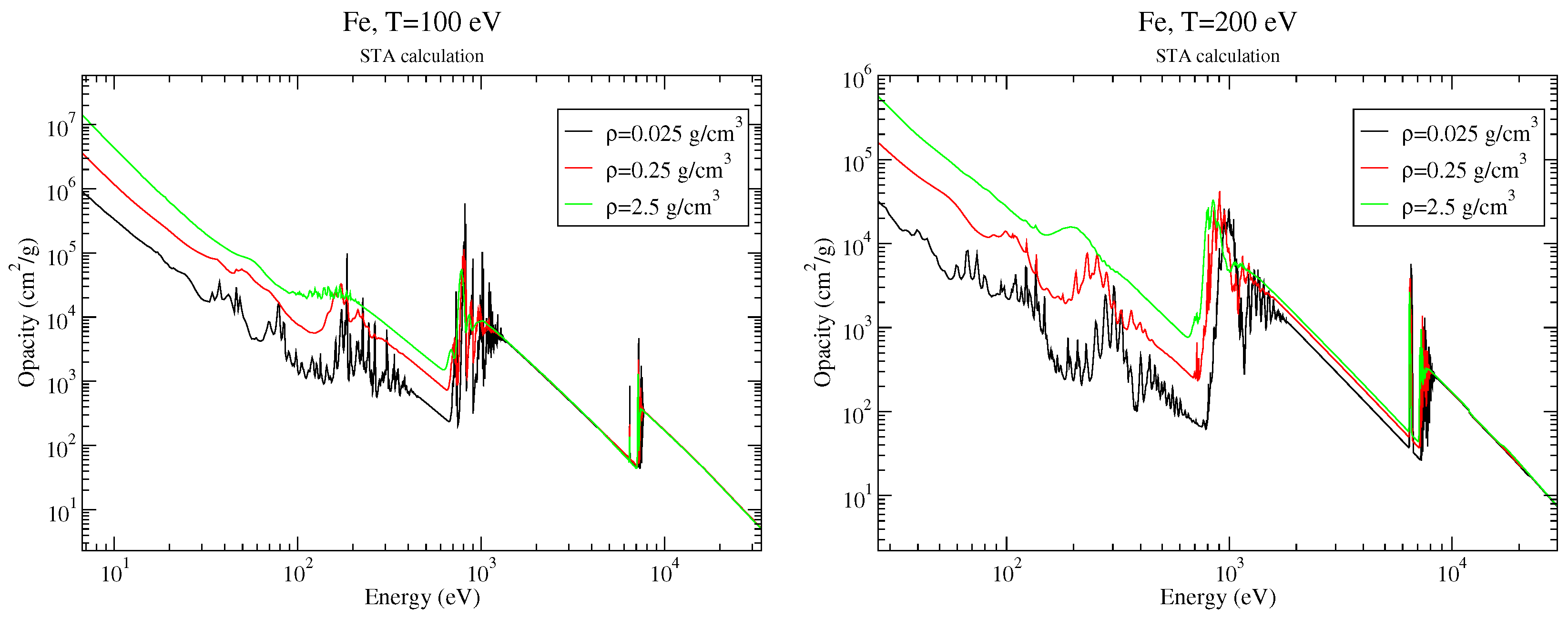
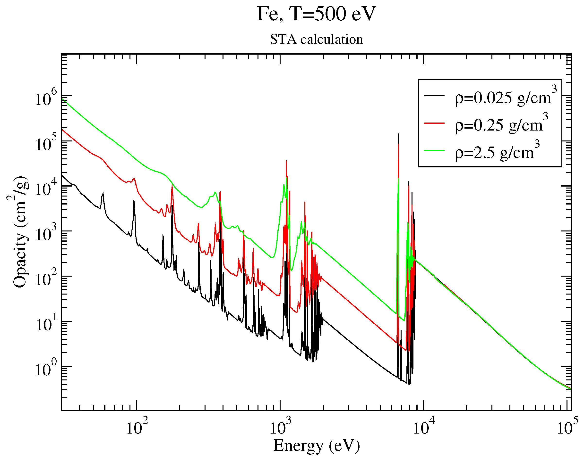
Figure 1 and Figure 2 represent the opacity of an iron plasma at = 0.025, 0.25, and 2.5 g·cm−3 and T = 100, 200 (Figure 1), and 500 eV (Figure 2), which were computed by code relying on the Super Transition Arrays formalism [18,19,20,21]. The detailed structure of the spectrum becomes more visible when the density decreases because the line widths become smaller, which reduces the overlap between line shapes. Throughout this paper, when anything other than “opacity” is mentioned, it refers to “spectral opacity”, i.e., opacity as a function of photon energy. When it is an average opacity (Planck or Rosseland, for instance), it is specified.
In order to take into account the plasma dispersion effect and multiple collisions, Equation (4) should read
where represents the refractive index, whose square can be approximated as [22,23]:
where denotes the collision pulsation and is the plasma pulsation (, where is the reduced Planck constant).
2.2. From the Schwarz Inequality to the Bernstein and Dyson Bound
The latter expression comes from the well-known Thomas–Reiche–Kuhn oscillator strength sum rule [25,26,27,28,29]. Z is the atomic number, is the Avogadro number, m is the electron mass, and A is the molar atomic mass. This leads to [30]:
where we have used the fact that , with being the Apéry constant (and the Riemann zeta function).
2.3. Relation between Planck and Rosseland Means
The Planck mean opacity reads
We have
Setting this time and , one obtains
leading to
which was obtained by Armstrong [15]. However, since the Planck mean is often significantly larger than the Rosseland mean, this relation is not really constraining.
2.4. Hölder Inequality
2.5. Introduction of an Alternative Mean Opacity
Setting and in the Schwarz inequality, one obtains
i.e.,
where we define the “Milne opacity”:
2.6. Milne Inequalities for Mixtures
Starting from the second Milne inequality (see Equation (21)), in the case of a mixture of two components, setting and , one has
Applying the Schwarz inequality with and , we obtain
This result can be generalized to the case of n constituents and one has
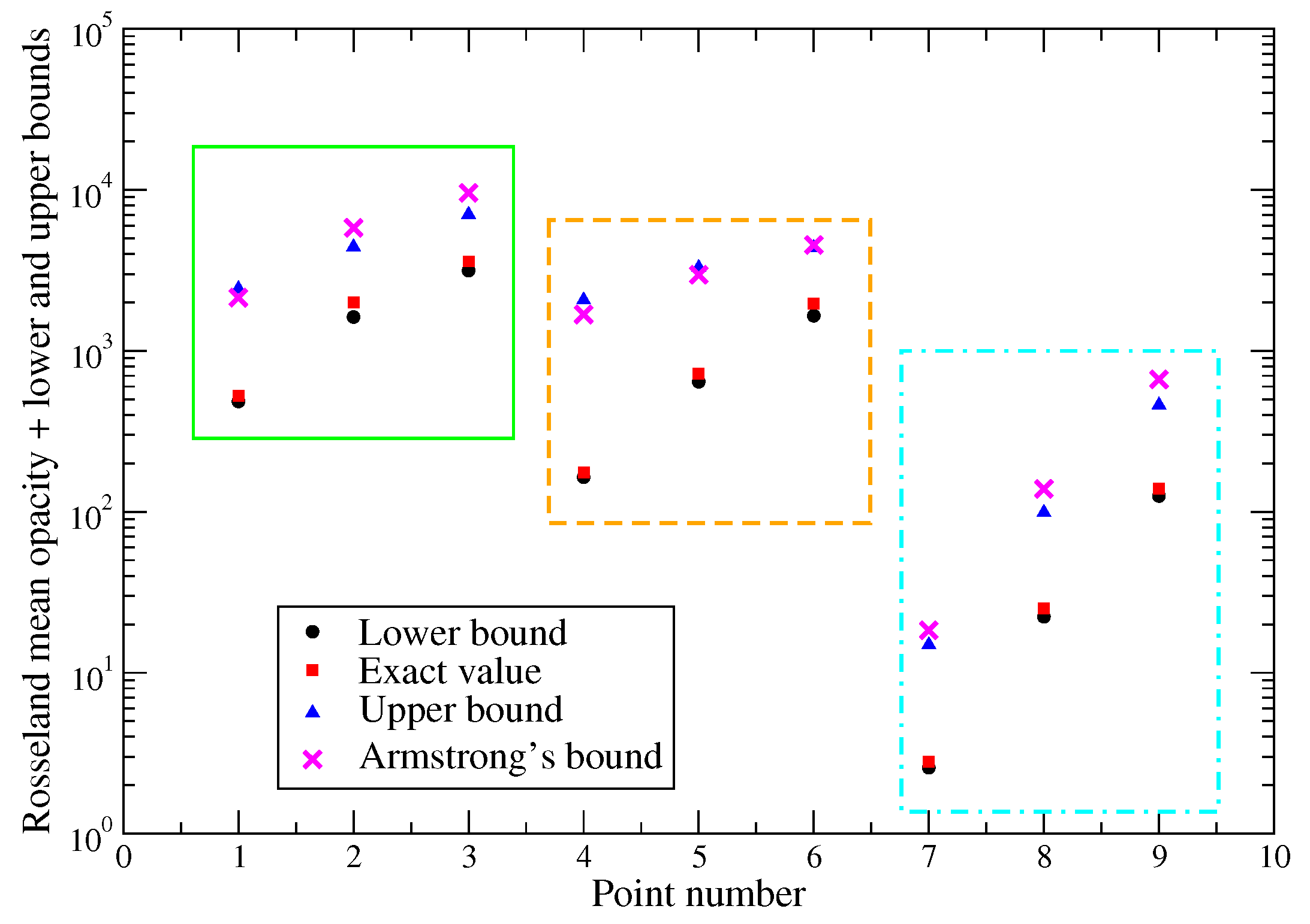
Table 2 contains the Rosseland, Planck, and “Milne” (see Equation (19)) mean opacities for an iron-magnesium plasma at different temperatures (100, 200, and 500 eV) and densities (0.025, 0.25, and 2.5 g·cm−3). The value of Armstrong’s bound (1.05349 ) is also specified. We can see that the Milne opacity is smaller than Armstrong’s bound for the two highest densities at T = 100 eV, the highest density at T = 200 eV, and the three densities at T = 500 eV.
Table 3 contains the partial densities of iron and magnesium for a mixture plasma (number fractions of Fe and Mg are both equal to 0.5) at different temperatures (100, 200, and 500 eV) and densities (0.025, 0.25, and 2.5 g·cm−3). These partial densities are obtained by applying the same electronic pressure to all ions in the plasma [33,34]. Table 4 and Table 5 present the partial Rosseland and Planck means of iron and magnesium, respectively (i.e., the opacities of the latter constituents at the partial densities obtained from the above-mentioned mixture model).
Table 6 shows the values of the partial “Milne opacity” for iron and magnesium in the mixture. Table 7 displays a comparison of the Rosseland mean opacity and lower bound from Equation (24). We can see that in each set of thermodynamic conditions, the two values are rather close, which means that this lower bound may be constraining and useful.
Figure 3 presents a comparison of the exact Rosseland mean, the two bounds provided by Equation (24), and Armstrong’s bound in the case of an iron-magnesium mixture plasma at three different temperatures, 100, 200, and 500 eV, and three different densities, 0.025, 0.25, and 2.5 g·cm−3. As in the pure iron case, the Armstrong bound is significantly higher than the exact value. The Milne opacity bound is sometimes more constraining but is still much higher than the exact value.
We have chosen the iron-magnesium opacity as an example since it is relevant to the pioneering Z-pinch experiments performed at Sandia [35], showing an important discrepancy between experiment and theory. The mathematical inequalities presented here can be useful for assessing the relevance of the experimental spectrum. However, it is important to remain cautious; indeed, the experiment concerns only a narrow photon-energy range and the inequalities considered in the present work involve integrals over the whole photon-energy range (from 0 to “infinity”). The purely mathematical inequalities (Schwarz, Hölder, etc.) can be applied over a limited energy band but the Thomas–Reiche–Kuhn oscillator strength sum rule can be applied only over the entire range. Iglesias pointed out that the measurements appear to violate the sum rule but his analysis relies on a comparison with the “cold opacity”, leading him to conclude that since the main absorption features from the L shell are in the experimental range, the number of electrons in that shell would be inconsistent with the mean ionization (and even potentially larger than the degeneracy!) [36]. This may be true but it is questionable because the Thomas–Kuhn–Reiche rule is valid for isolated-atom oscillator strengths and does not account for plasma effects and line shapes.
2.7. A New Bound: Compton Scattering and Inverse Bremsstrahlung
It is possible to derive new bounds without resorting to mathematical inequalities and oscillator strength sum rules, but rather by considering the fact that the spectral (monochromatic) opacity is a sum of several positive partial contributions. Two of them, the inverse Bremsstrahlung and the scattering contributions, can be approximated by analytical formulas. We have
and
where represents the scattering opacity (equal to its Rosseland mean ) in . We have seen that the Thomson opacity reads
The contribution of scattering can be refined by considering the Klein–Nishina cross-section instead of the Thomson one (see Appendix A). The Thomson and Klein–Nishina cross-sections mentioned above refer to the photon scattering by free electrons. Additional bounds can also be obtained using the low-energy Rayleigh scattering cross-section for neutral atoms, which can be derived from the static dipole polarizability of the neutral atom [37]. More detailed treatments are based on the dynamic (or frequency-dependent) dipole polarizability [38]. For instance, for oxygen, following the prescription of Ref. [39], one can take the following cross-section ( = 6.65246 · 10−25 cm2 is the total Thomson scattering cross-section):
where represents the Rydberg constant. The latter formula was rescaled so that the first term agrees with more accurate static dipole polarizability factors from Schwerdtfeger [40]. Assuming , the inverse of the cross-section (or opacity) can be expanded in series and it is possible to derive subsequent opacity bounds using the following integral
3. Detection of Errors: Benford and the Law of Anomalous Numbers
3.1. Generation and Development
In 1881, Newcomb, an American astronomer and mathematician, first discovered the law of the first digit. Through statistical analysis of the data, he pointed out that many numbers characteristic of nature can be expressed in an exponential form and that the logarithm of the index mantissa is uniformly distributed [42]. Benford discovered the same phenomenon and conducted deep research on 20,229 digits in more than 20 data sets appearing randomly in physical and chemical constants, prime numbers and Fibonacci numbers, and river lengths and lake areas. He arrived at the same conclusions as Newcomb and proposed the formal “first digit law” [43], arousing the interest of many scientists. This law was later named after him [44]. In the following forty years, the development of basic research was very slow. Although the related research explained some of the properties of Benford’s law, it was not proved from a mathematical point of view. Hill proved that the first digit obeys Benford’s law [45] and is consistent with the central limit theorem. In addition, he generalized the theory, obtained the distribution function law of higher-order digits, and derived the joint distribution function between the first digit and the higher-order digits.
Thus, Benford’s law means that the significant digits of many sets of naturally occurring data are not equi-probably distributed, but rather in a way that favors smaller significant digits through a uniform logarithmic distribution. For instance, the first significant digit, i.e., the first digit that is non-zero, will be 5 more frequently than 6, and the first three significant digits will be 548 more often than 576.
The verification of the usability (applicability verification) of Benford’s law has been checked in different fields [46]. For instance, relevant research has been carried out in the fields of economics, sociology, physics, computer science, and biology. Among them, the most influential research is the systematic applicability of Benford’s law to the detection of tax fraud [47]. It was found through statistics that computer file size [48], biological protein domain length, popular survival distribution [49], spectrum line strength [50,51] in complex atomic spectroscopy, hadron lifetime, or the energy loss rate of pulsar self-rotation slowing [52] all accurately verified the law. Even the distributions of distances of galaxies and stars conform to Benford’s law [53]. In number theory, it was shown that Jacobsthal, Jacobsthal–Lucas, and Bernoulli numbers follow the law [53]. This is the case for other families of numbers such as Mersenne numbers [54]. However, many data sets have not passed the applicability verification such as the resident identity number or the height of an adult. Yunxia studied the important economic data of the national development zones in China and found that some numbers were inconsistent with the predictions of Benford’s law [55].
However, it is not always the case that Benford’s law is obeyed by data distributions and some data sets violate the law. These data sets can be roughly classified into two categories, one in which the data do not satisfy the objective condition for applying the law and the other containing anomalous data that break the law. For the former, the current theoretical basis cannot determine a reasonable data set a priori and it still needs to be judged by rigorous statistical analysis, which is its limitation. For the latter, scientists skillfully use this feature to develop Benford’s law as an effective tool for assessing data quality and mining anomalous data.
Benford proposed a probability distribution function for significant digits, which states that the probability that the first significant digit is equal to k is given by [43]:
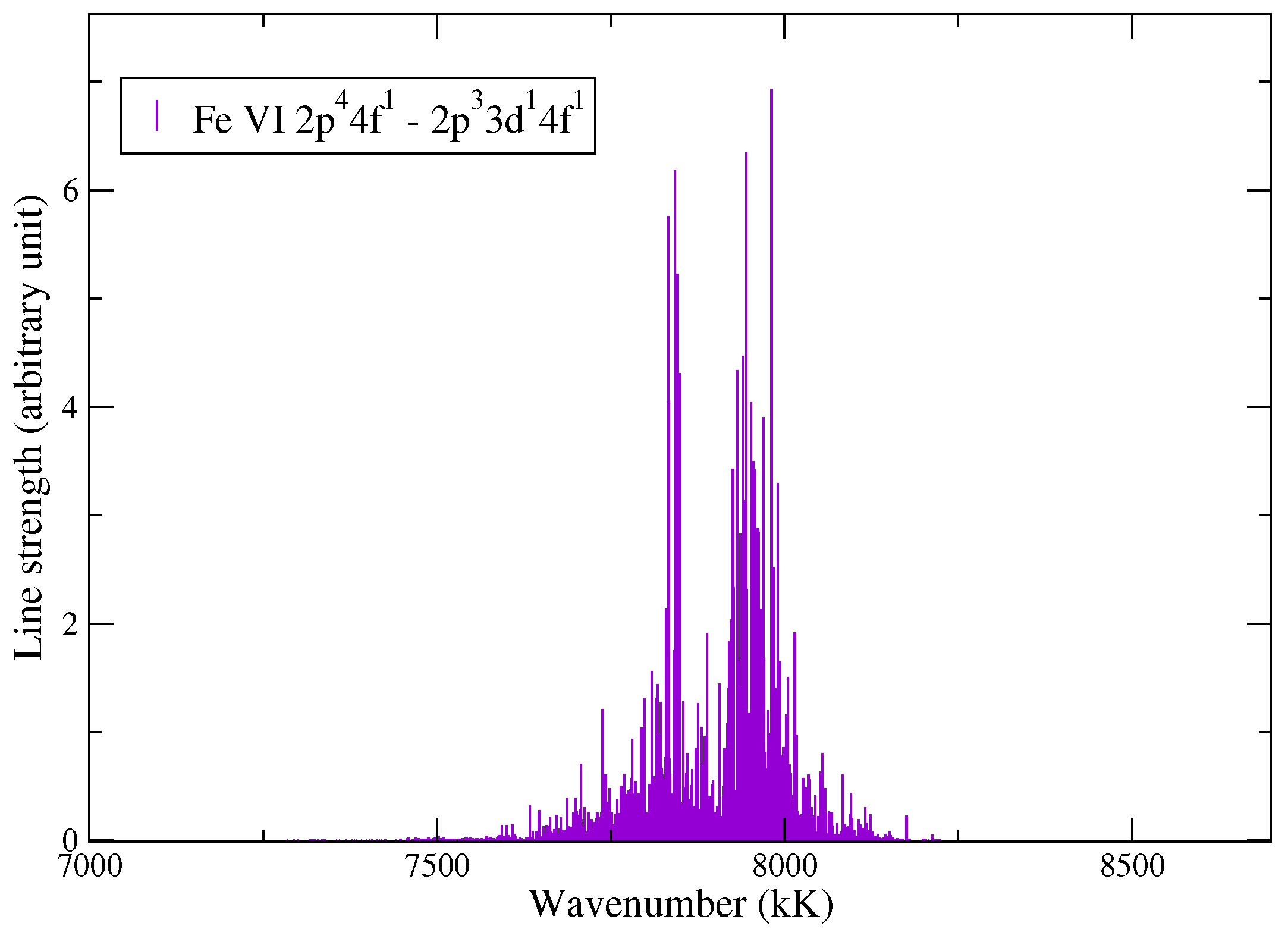
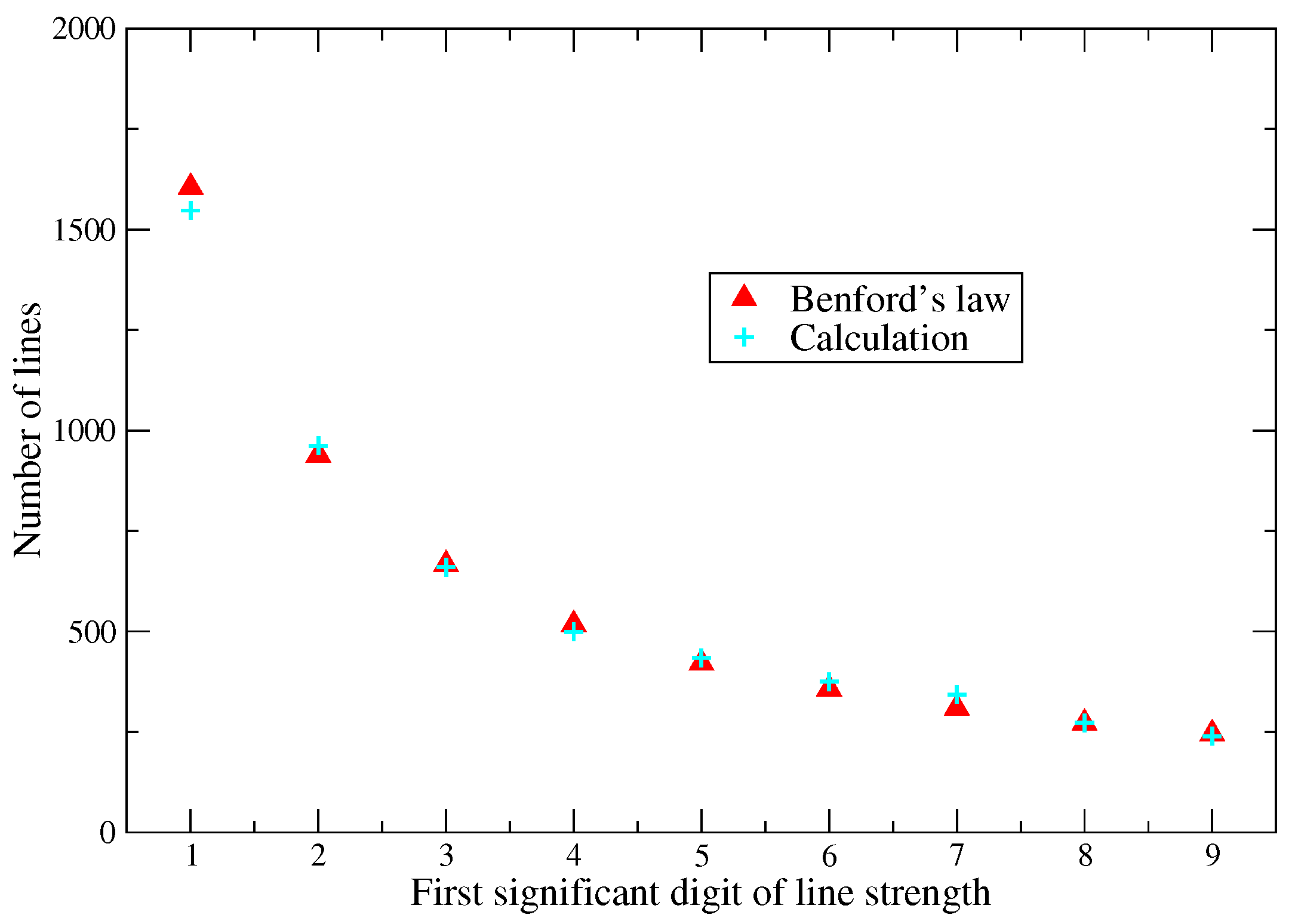
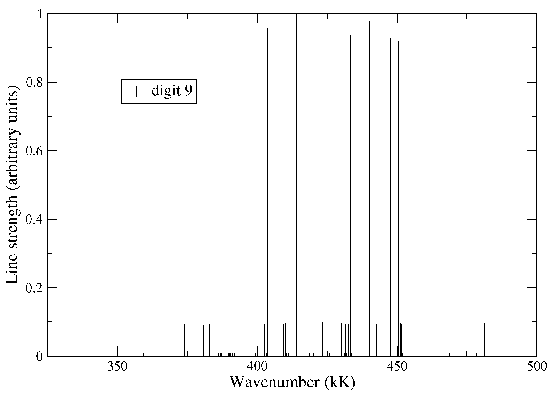
As mentioned above, it was noticed (see Ref. [50]) that the distribution of lines in a given transition array follows Benford’s logarithmic law of significant digits very closely (see Figure 4 and Figure 5 for the transition array of Fe VI (Fe5+) computed with Cowan’s code [56]). This indicates that the distribution of digits reflects the symmetry due to the selection rules. If transitions were governed by uncorrelated random processes, each digit would be equi-probable. An interesting point is that the lines of a non-relativistic transition array seem to follow Benford’s law even when the spin–orbit interaction is important. The values from Figure 5 are provided in Table 8.
In the latter table, the error is defined as
We can see that the error is always very small (below 3%) and that there is no systematic rule in the sense that the distribution of digits in the data can be either lower or higher than the prediction of Benford’s law.
3.2. Explanations
3.2.1. Multiplicative Stochastic Processes
Benford’s law is still not fully understood mathematically. However, it can be applied if the system is governed by random multiplicative processes [57], i.e., processes that are additive in a logarithmic space. In Wigner’s Random Matrix Theory (RMT) [58], the Hamiltonian is defined in the Gaussian Orthogonal Ensemble (GOE) by an ensemble of real symmetric matrices whose probability distribution is a product of the distributions for the individual matrix elements, considered stochastic variables, and the variance of the distribution for the diagonal elements is twice that of the off-diagonal elements. The matrix elements of the Hamiltonian are correlated stochastic variables and the product of these variables, arising through the diagonalization process, leads to Benford’s logarithmic distribution of digits. Since Benford’s law can be explained in terms of dynamics governed by multiplicative stochastic processes (additive in logarithmic space), RMT is a relevant and well-suited tool for the calculation of large E1 transition arrays [59] and Benford’s law can help to clarify the existence of different classes of stochastic Gaussian variables.
3.2.2. Scale Invariance
Although the previous explanations show the kind of data that would conform to Benford’s law, scale invariance explains how the formula can be derived. If the first digits of some large data sets conform to a particular distribution, the latter distribution must be independent of the data’s units of measurement. Let us consider that variable x follows a scale-invariant distribution and assume that . Then, multiplying x by a constant, i.e., adding a constant to , does not change the distribution. The only distribution invariant when a constant is added is the uniform distribution U. This means that in the interval [1–10]:
and, therefore, . Then, we have
It is important to mention that Hill also showed that base invariance implies Benford’s law [60].
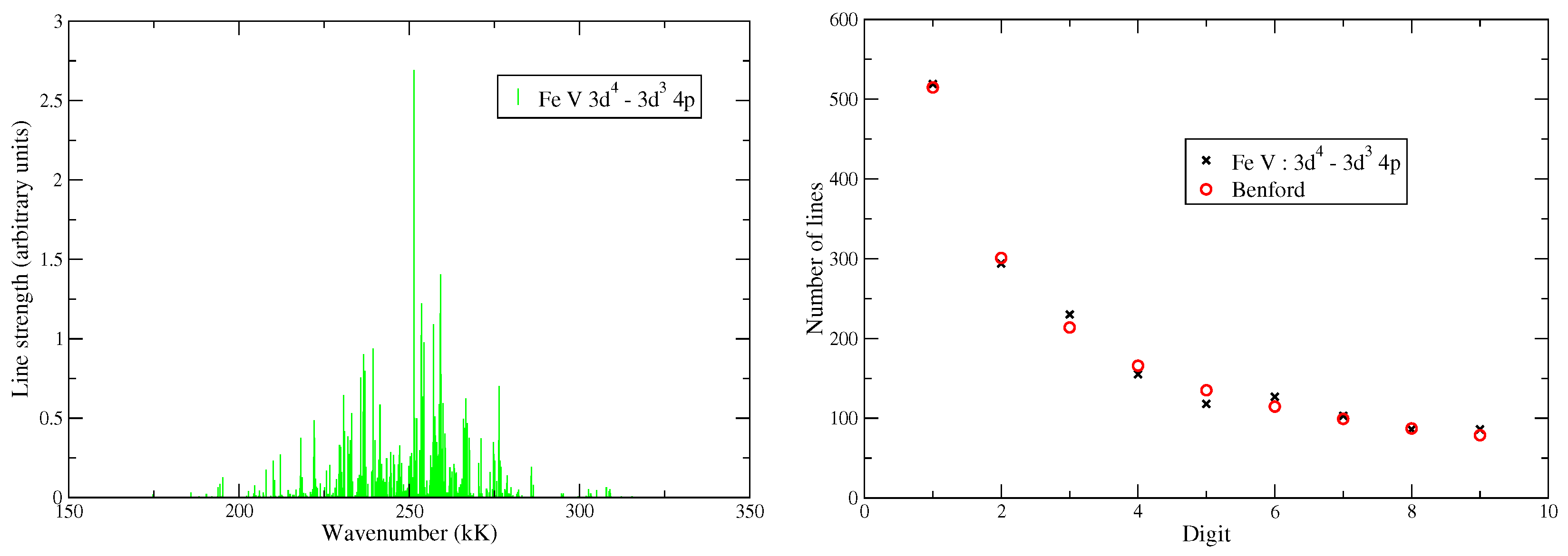
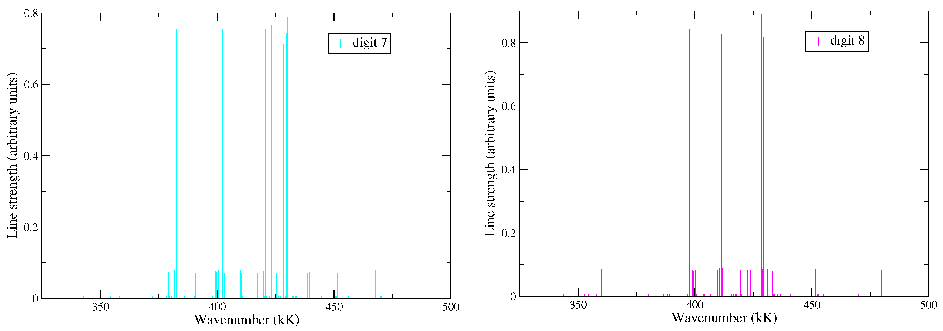
It is interesting to take a look at different transition arrays and different charge states. Figure 6 and Figure 7 show the results for transition arrays and , Figure 8 and Figure 9 focus on transition arrays and , and Figure 10 and Figure 11 focus on transition arrays and . We can see that although the transition arrays have very different shapes, Benford’s law always applies with great accuracy. Some small discrepancies can be observed, for instance, in the case of digit 8 for (Figure 7, right) or for digits 2 and 4 in the case of (Figure 11, right). It is expected that the higher the statistics, the higher the likelihood that the law will be verified, but it seems that even for transition arrays with the smallest numbers of lines, the results are very convincing.
The fact that the line strengths follow Benford’s law, which is a consequence of scale invariance, is consistent with the fact that the distribution of the lines presents a fractal nature, as we have seen in Section 3.
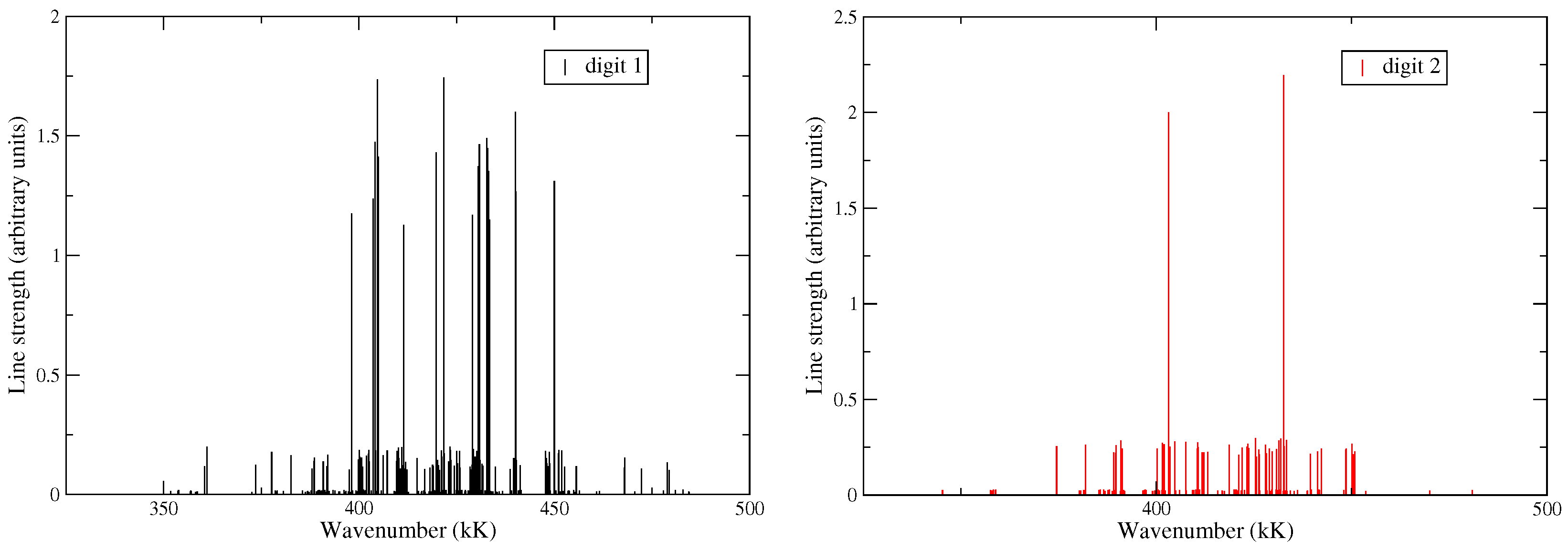
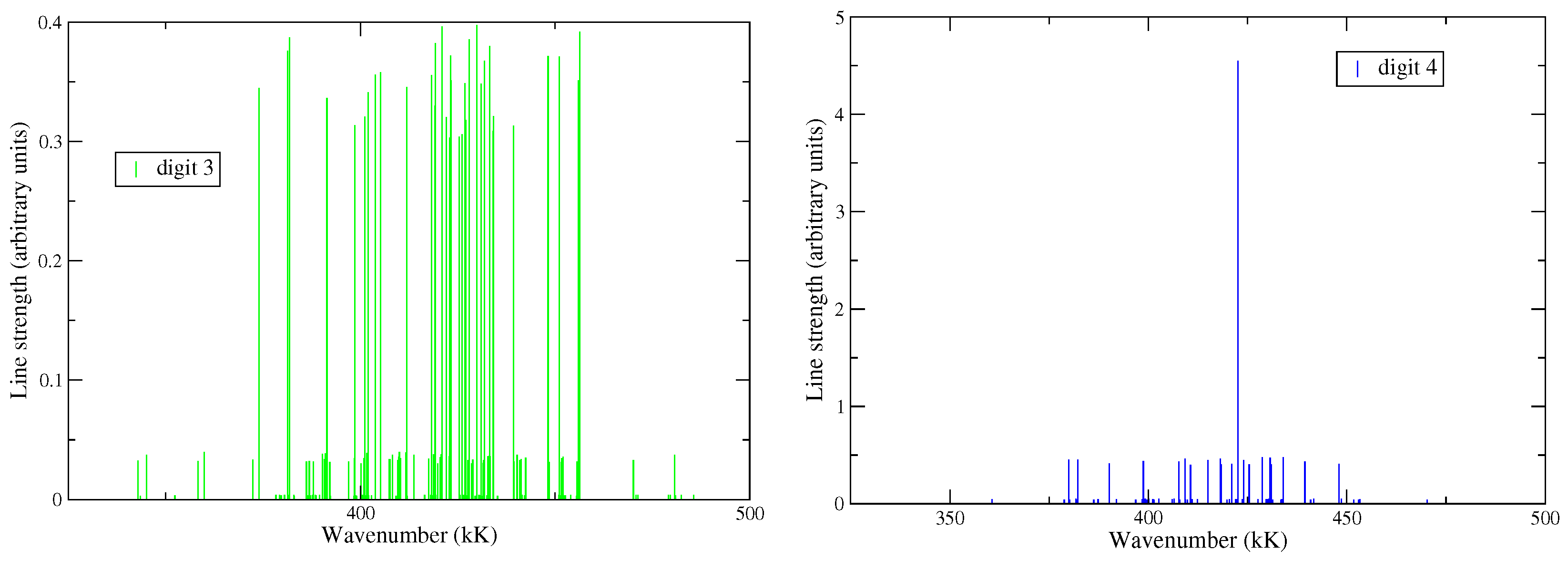
It is interesting to see how the energies are distributed with respect to the first significant digit of their strength (see Figure 12, Figure 13, Figure 14, Figure 15 and Figure 16). We can see that the energies of the weak or intermediate-strength lines are widespread over the energy range of the transition array and that the strongest lines are gathered into a very limited number of bunches, which are located close to the center of the transition array. This is a consequence of the propensity rule and strength–energy correlation. The former means that the arrays are much narrower than the configurations (in the absence of a correlation, the energy variance of an array would be equal to the sum of the variances of the configurations). The propensity rule is the trend of a line to connect preferentially a low (respectively, high)-energy level of the initial configuration to a low (respectively, high)-energy level of the final configuration. The strength–energy correlation implies that the strongest lines are close to the center of the array. The energy–amplitude correlation is such that, when the spin–orbit interaction is weak, the general trend of an array is to gather the strongest lines close to its center and disperse the weakest lines to its edges. Due to these two effects, a transition array is expected to be sharp [61,62].
3.3. Improvement Methods
The test accuracy in the application of Benford’s law can be improved in three aspects: expanding the scope of the test, combining it with other models, and strengthening the analysis of the test results.
In order to improve the efficiency of the data verification process, it is important not to limit the analysis to the first digit and to extend the analysis to the next digits. For instance, Benford’s law states that the first digit will be 2 more often than 5, but also that the first two digits will be 54 more often than 55, 546 more often than 548, etc.
- In general, the quality of the data set with the first digit obeying Benford’s law is good, but when the distribution probabilities of different digit combinations (such as the first-second, second-third, first-third digits, etc.) conform to the law, the test results are even more accurate.
- “Multi-dimensional” detection data. If the conclusions of several tests (concerning different relevant quantities of the system) are consistent, the data can be considered reliable.
If the law is violated in a line-strength database, it means that there is something wrong but it does not give any insight into the precise nature of the problem. It does not indicate which line strengths are wrong or why. It may be a writing format issue, a bug in the code occurring only for specific orders of magnitude, a numerical problem affecting only very small or very large values, etc. Most codes combine different approximations, some of which may be inappropriate and concern only values in a narrow range of a given decade, having the same first significant digit. If one were to conduct line-strength calculations with a variety of structure codes, one could assess the consistency and/or correctness of these codes through the application of Benford’s law. In this sense, Benford’s law is not a diagnostic tool stricto sensu, but rather an indicator of the reliability of a database.
4. The Learner Rule
Learner measured a large number of line intensities in the atomic spectrum of neutral iron and in 1982, demonstrated the existence of a remarkable power law for the density of lines versus their intensity [63]: the logarithm of the number of lines , whose intensities lie between and (n is an integer), is a decreasing linear function of n:
where L is the total number of lines, is a constant, and is the slope (p being positive).
The value of is chosen in such a way that this law holds for 9 (9 octaves) when about 1500 lines within 290 nm 550 nm are considered. One has
where : the number of lines is multiplied/divided by when the size of the interval is multiplied by two.
Learner observed that if is the number of lines with intensity in octave k,
is computed through [61]
where represents the intensity distribution. Equation (39) is consistent with a distribution . For fractal objects [64], the measured length may depend on the length of the measure:
where L is the length of the object, ℓ is the measure, K is a constant, and D is the fractal dimension. In the present case, we choose for the number of lines whose intensity is larger than ℓ:
and neglecting , one finds .
Recently, Fujii and Berengut reported that the combination of two statistical models—an exponential increase in the level density of many-electron atoms [65] and local thermodynamic equilibrium excited-state populations—produces a surprisingly simple analytical explanation for this power law dependence [66].
They found that the exponent of the power law is proportional to the electron temperature. This dependence may provide a useful diagnostic tool to extract the temperatures of plasmas of complex atoms without the need to assign lines.
5. Quantifying the Precision of Interpolations
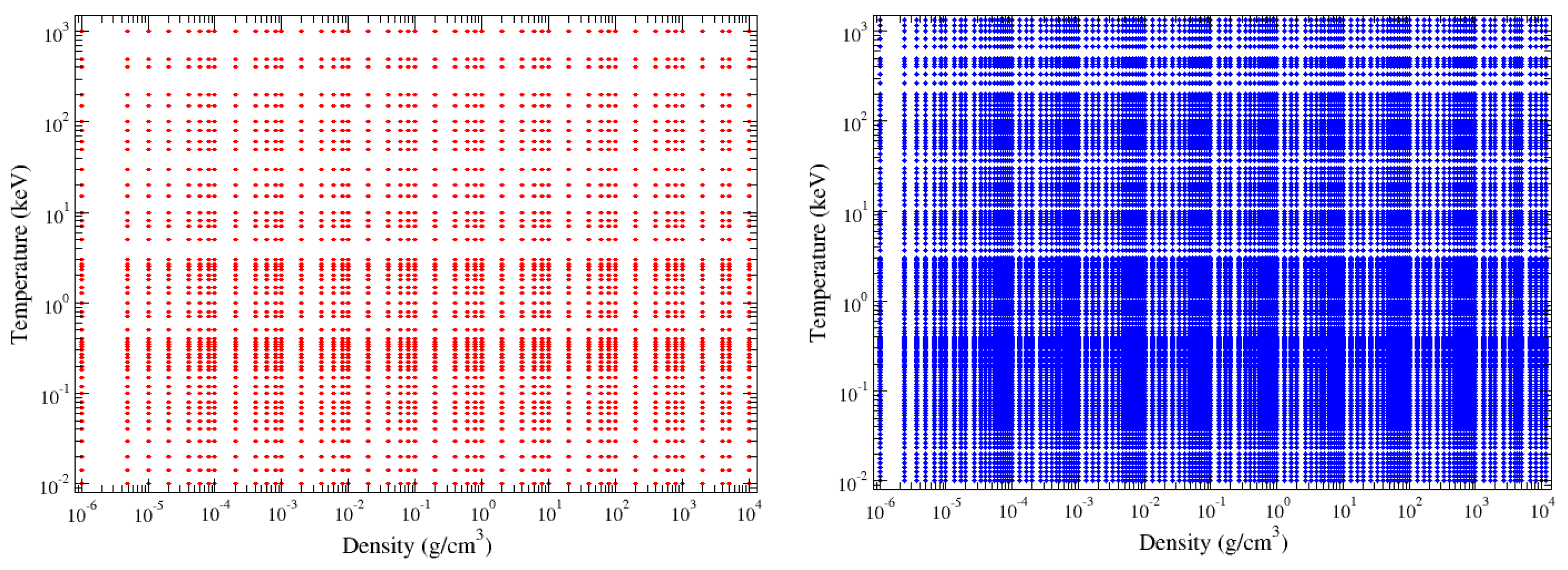
We compare two grids covering wide ranges of temperatures and densities; the first one contains 2350 points and the second one contains 21,000 points (see Figure 17).
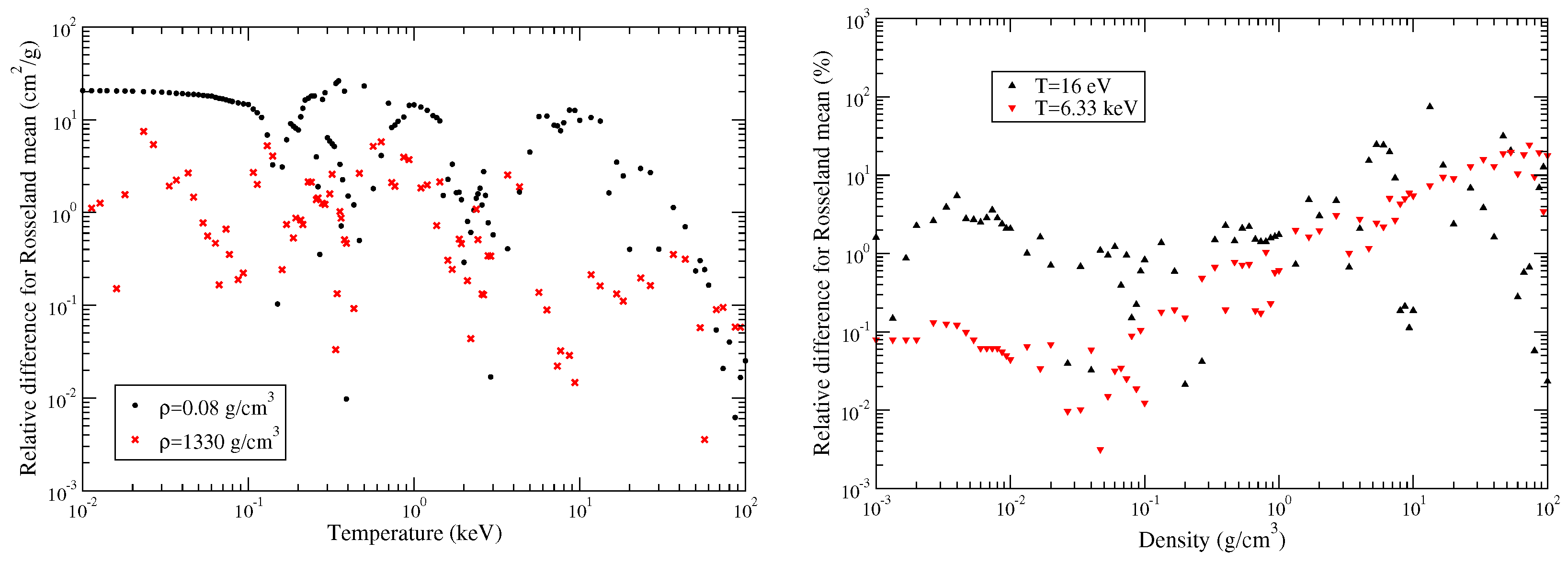
Figure 18 shows a comparison of the iron Rosseland mean opacity calculated on the dense grid (140 densities and 150 temperatures), and interpolated on it from a smaller grid, respectively, for two different densities, = 0.08 g·cm−3 and = 1330 g·cm−3, and two different temperatures, T = 16 eV and T = 6.33 keV, which were chosen because they were responsible for the most important discrepancies. Except for the latter cases, the differences rarely exceeded a few %.
6. Convergence with Respect to the Number of Superconfigurations
The STA model relies on the concept of superconfigurations. A superconfiguration is an ensemble of configurations close in energy. For instance,
is a superconfiguration made up of five supershells, , , , , and , populated, respectively, with 2, 4, 5, 3, and 2 electrons. For instance, represents all the possibilities of distributing 5 electrons in and , i.e., the number of pairs such that and and . The superconfiguration S represents
ordinary configurations, such as
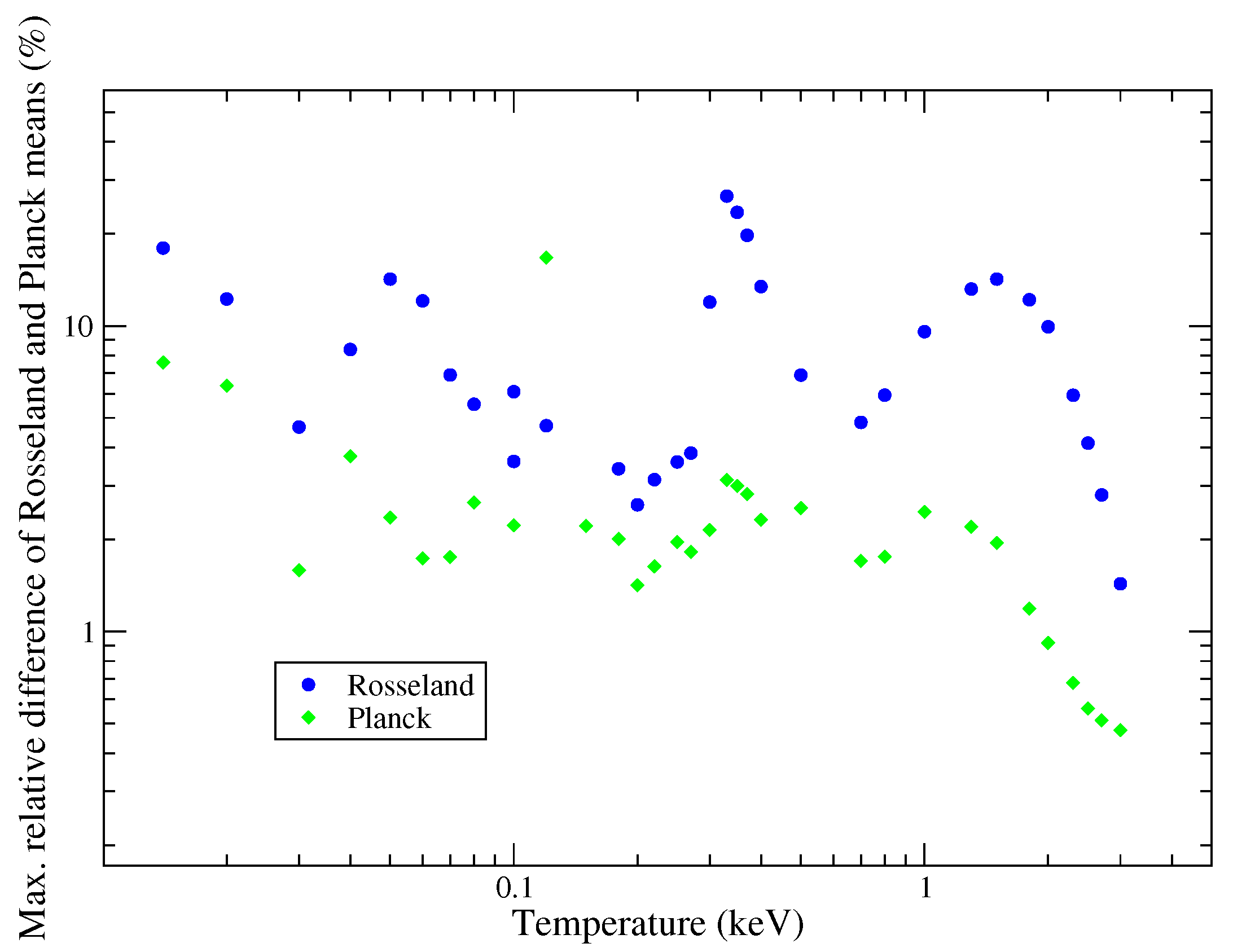
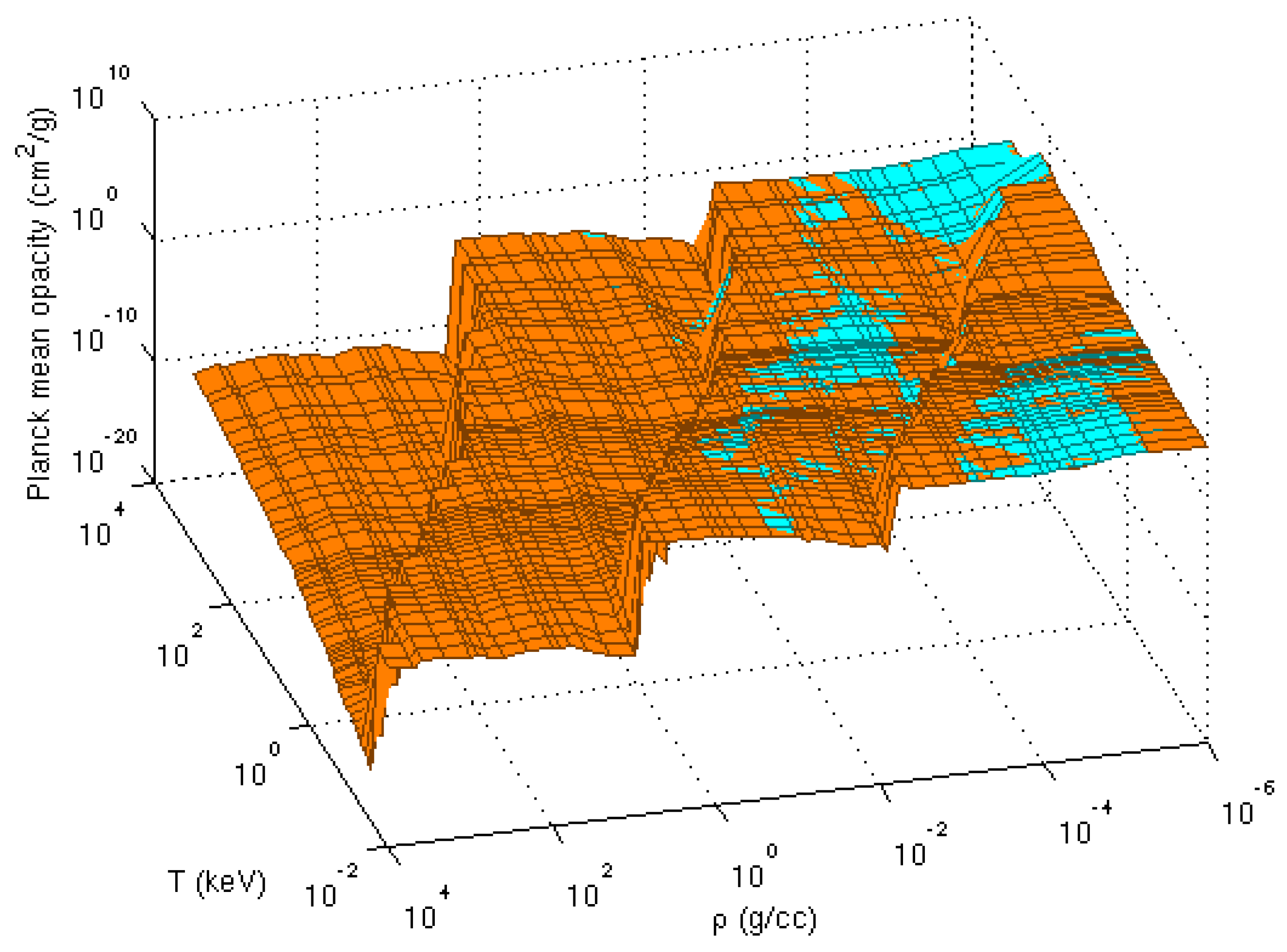
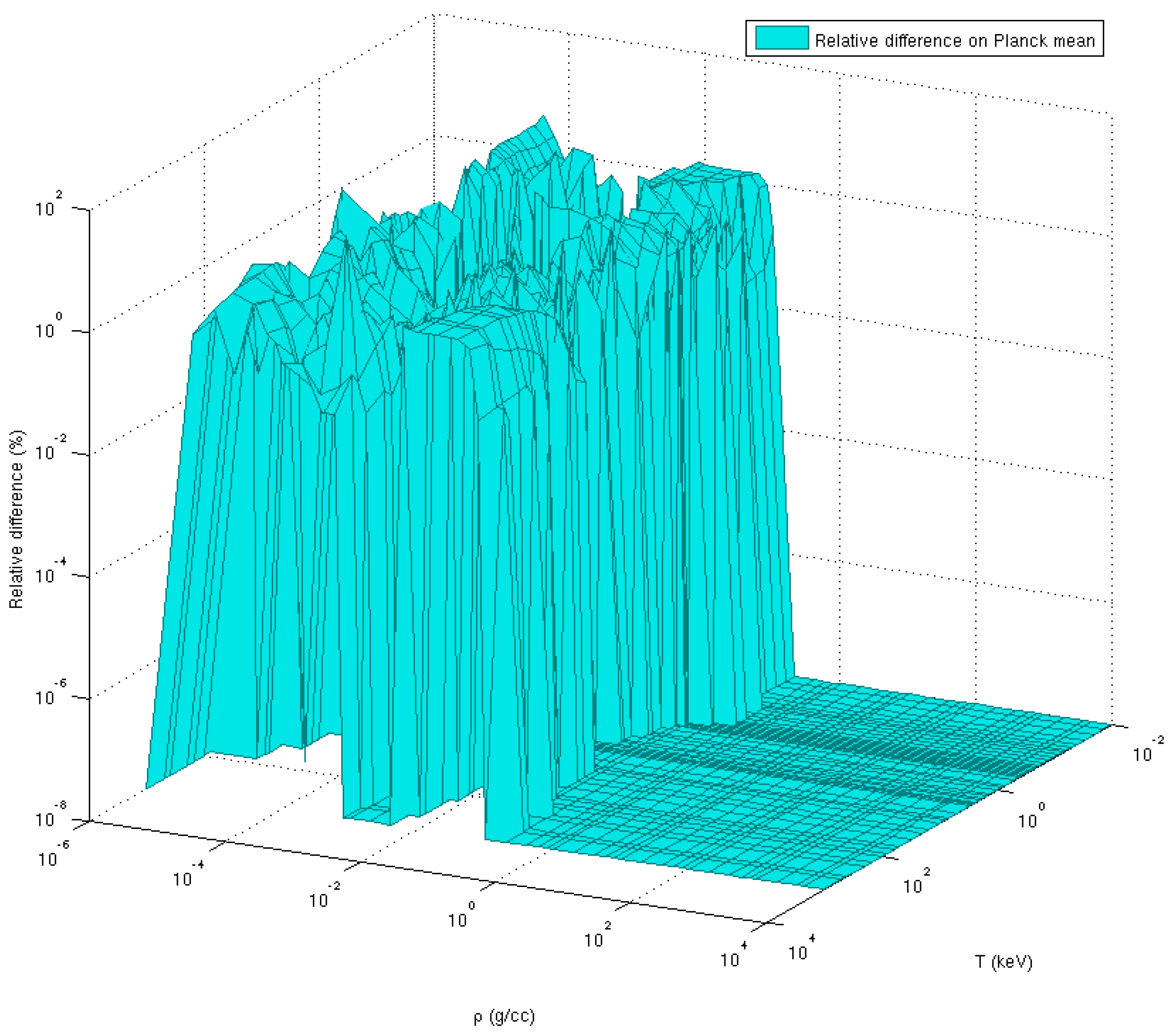
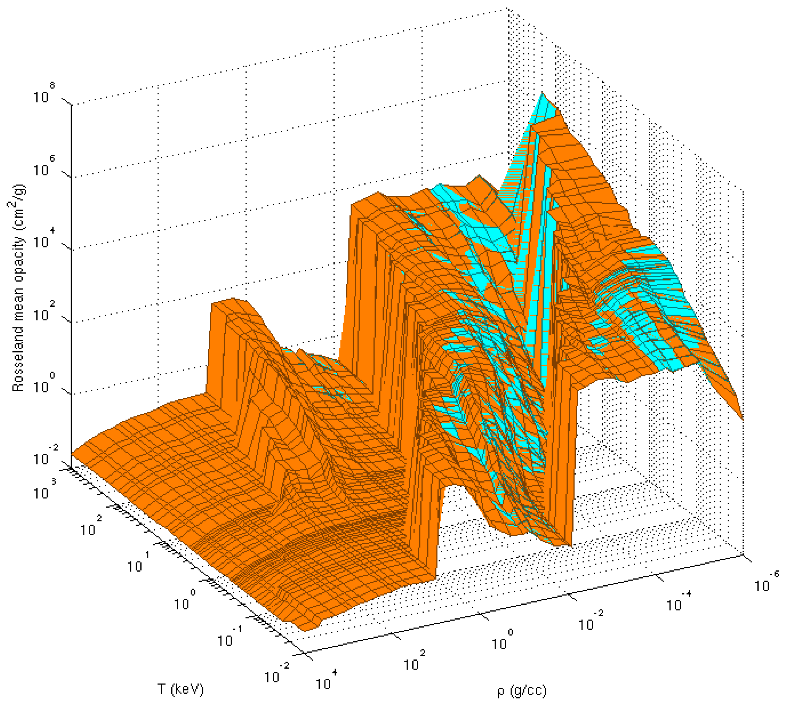
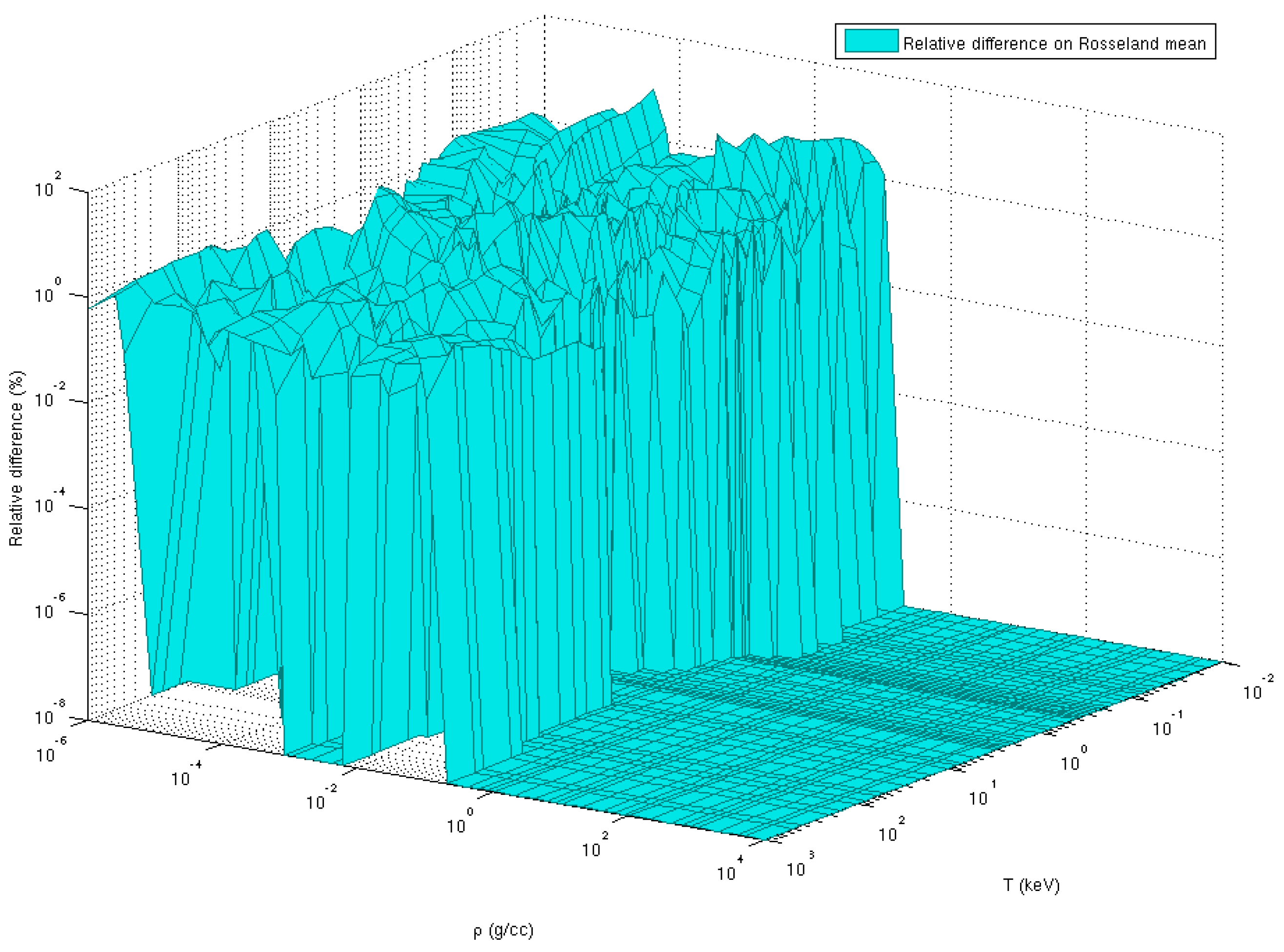
We compare the cases with 1000 and 10,000 superconfigurations. Figure 19 shows the maximum value of the relative difference (in absolute values) between the iron Planck and Rosseland mean opacities of a calculation with a maximum number of 1000 superconfigurations and a maximum number of 10,000 superconfigurations as a function of temperature. Figure 20 represents the iron Planck mean opacities resulting from a calculation with a maximum number of 1000 superconfigurations and a maximum number of 10,000 superconfigurations as a function of temperature and density. Figure 21 displays the maximum value of the relative difference (in absolute values) between the iron Planck mean opacities of a calculation with a maximum number of 1000 superconfigurations and a maximum number of 10,000 superconfigurations as a function of temperature and density. Figure 22 shows the iron Rosseland mean opacities of a calculation with a maximum number of 1000 superconfigurations and a maximum number of 10,000 superconfigurations as a function of temperature and density and Figure 23 represents the maximum value of the relative difference (in absolute values) between the iron Rosseland mean opacities of a calculation with a maximum number of 1000 superconfigurations and a maximum number of 10,000 superconfigurations as a function of temperature and density. We can see that the relative differences can reach 30% for the Rosseland mean, which is very important. For the Planck mean, the maximum relative difference is smaller than that of the Rosseland mean and smaller than 10% (except for one value) of the temperature range considered in Figure 19. It is worth noting that the global variations are the same for both opacity means. The most important differences occur at a high temperature and moderate density, where the number of excited states is important. A low density means a large Wigner–Seitz radius and therefore more allowed subshells of high principal n (and subsequently orbital ℓ) quantum numbers, and a high temperature implies that high-lying states can be populated by electrons. However, as can be seen in the three aforementioned figures, things are a bit more complicated; this is a general trend. It is also important to be careful with the interpretation of Figure 19 since only the maximum relative difference (over all densities) is represented for a given temperature. The fact that the maximum relative difference for a temperature is larger than that for a temperature does not mean that the average difference at (over all densities) is more important than the average difference at .
7. Perspectives
Starting from an oscillator strength sum rule, Imshennik et al. derived an integral relation that must be satisfied by the bound-electron radiation absorption coefficient when the distribution of ions with respect to the degree of ionization and excitation state is arbitrary. Making use of this relation, the authors formulated and solved a variational problem that, under the conditions of local thermodynamic equilibrium (LTE), yielded the smallest possible value of the Rosseland mean free path, i.e., the largest possible value of the Rosseland opacity [67].
In a similar vein, Molodtsov et al. constructed a complete set of estimates for the maximal Rosseland mean opacity for an LTE plasma with an arbitrary ion distribution in terms of the degree of ionization and state of excitation on the basis of quantum-mechanical sum rules of the kind
The case is a direct consequence of the Thomas–Reiche–Kuhn sum rule and is equal to the number of electrons in the atomic system. The case can be expressed through the mean square radius of the atom in the ground state, the sum can be expressed through the mean square momentum of the electron in the ground state, and the sum can be expressed in terms of the density of the electrons at the nucleus [68].
8. Conclusions
We have investigated a few aspects of atomic physics (and more specifically opacity) databases. We have seen that mathematical inequalities combined with oscillator strength sum rule(s) can be helpful for checking the relevance of compiled data or experimental results. Additional mathematical inequalities likely to provide new bounds are provided in Appendix B. In a different framework, Benford’s law is known to be an efficient tool for testing data quality in different fields of nature, social sciences, etc. It sheds light on the strategic role of big data in the modern era and supports governments and industry leaders in making scientific decisions. The purpose is not only to judge the quality of data but also to mine anomalies and extract effective information. It was shown a few years ago that Benford’s law was verified by line strengths in atomic spectra. The understanding of its theoretical grounds should be deepened and its applicability conditions clarified. Moreover, the joint application of Benford’s law and other data processing techniques should be strengthened according to the common data quality problems in atomic physics computations. This could be performed by adopting data mining techniques (classification, clustering, outlier detection), traditional data detection models, and other targeted optimization test methods. There are inevitable or accidental errors in the data verification process. An important method for improving the accuracy of the test results is to adopt appropriate methods for avoiding, eliminating, or correcting the errors. The development of Benford’s law in the future will require specialists from all fields to further study its essence, strengthen its integration with other data processing technologies, and then expand its applications. All the ideas presented here may also be of great interest for checking molecular-opacity databases [69]. These constraints can also be useful for assessing the reliability of an experimental measurement [70,71].
Author Contributions
J.-C.P. and P.C. developed the theory, carried out the analytic calculations and performed the computations. J.-C.P. wrote the first version of the manuscript. All authors have read and agreed to the published version of the manuscript.
Funding
This research received no external funding.
Institutional Review Board Statement
Not applicable.
Informed Consent Statement
Not applicable.
Data Availability Statement
The data presented in this study are available on request from the corresponding author. The data are not publicly available due to privacy and ethical restrictions.
Acknowledgments
J.-C.P.: I am indebted to Freeman J. Dyson for their fruitful correspondence about the subject in 2016. Dyson took much time to give me advice and suggestions of paths to explore. This was a great honor for me. J.-C.P. and P.C.: We express our gratitude to J.-P. Raucourt, V. Tabourin, and A. Fontaine for their computational support in the generation of the high-resolution opacity tables. We also thank the anonymous referees for their helpful comments and suggestions.
Conflicts of Interest
The authors declare no conflict of interest.
Abbreviations
The following abbreviations are used in this manuscript:
| GOE | Gaussian Orthogonal Ensemble |
| LTE | Local Thermodynamic Equilibrium |
| NIF | National Ignition Facility |
| RMT | Random Matrix Theory |
| STA | Super Transition Arrays |
Appendix A. Klein–Nishina Scattering Rosseland Mean
Introducing the reduced parameter , the Klein–Nishina relativistic cross-section reads
If , one has
and if
Let us assume that the relativistic effects are negligible. We can then take Equation (A2), yielding
Using the reduced variable , one has for the Rosseland mean, in the case of the Klein–Nishina expression of the scattering cross-section,
i.e.,
Using
as well as
and
we get
i.e.,
Appendix B. Additional Mathematical Inequality Likely to Provide New Bounds
Other mathematical inequalities may also be of interest [72] such as the Minkowski inequality [73,74] or the Jensen convexity inequality [75]. The Pólya–Szegö inequality [76,77,78], which states that if and , then
could lead to new constraints, as well as the following ones published by Karamata [79]:
and
with
or the Young inequality [80]:
with, as in the Hölder inequality,
References
- Hui-Bon-Hoa, A. Stellar models with self-consistent Rosseland opacities–Consequences for stellar structure and evolution. Astron. Astrophys. 2021, 646, L6. [Google Scholar] [CrossRef]
- Seaton, M.J.; Yan, Y.; Mihalas, D.; Pradhan, A.K. Opacities for stellar envelopes. Mon. Not. R. Astron. Soc. 1994, 266, 805–828. [Google Scholar] [CrossRef]
- Iglesias, C.A.; Rogers, F.J. Updated OPAL opacities. Astrophys. J. 1996, 464, 943–953. [Google Scholar] [CrossRef]
- Krief, M.; Feigel, A.; Gazit, D. A New Implementation of the STA Method for the Calculation of Opacities of Local Thermodynamic Equilibrium Plasmas. Atoms 2018, 6, 35. [Google Scholar] [CrossRef]
- Mendoza, C. Computation of Atomic Astrophysical Opacities. Atoms 2018, 6, 28. [Google Scholar] [CrossRef]
- Pain, J.-C.; Gilleron, F.; Comet, M. Detailed Opacity Calculations for Astrophysical Applications. Atoms 2017, 5, 22. [Google Scholar] [CrossRef]
- Pain, J.-C.; Gilleron, F.; Comet, M. Detailed Opacity Calculations for Stellar Models. In Proceedings of the Workshop on Astrophysical Opacities, Michigan University, Kalamazoo, MI, USA, 1–4 August 2017; Mendoza, C., Turck-Chièze, S., Colgan, J., Eds.; ASP Conference Series. Astronomical Society of the Pacific: San Francisco, CA, USA, 2018; Volume 515, p. 35. [Google Scholar]
- Mondet, G.; Gilleron, F.; Pain, J.-C.; Calisti, A.; Benredjem, D. Opacity calculations in ICF plasmas. High Energy Density Phys. 2013, 9, 553–559. [Google Scholar] [CrossRef]
- Dyson, G.B. Project Orion; Henry Holt: New York, NY, USA, 2002. [Google Scholar]
- Bernstein, J.; Dyson, F.J. The Continuous Opacity and Equations of State of Light Elements at Low Densities; General Atomic Report GA-848; unpublished.
- Bernstein, J.; Dyson, F. Opacity bounds. Publ. Astron. Soc. Pac. 2003, 115, 1383–1387. [Google Scholar] [CrossRef]
- Huebner, W.F. Some estimates of the radiative Rosseland mean opacity. J. Quant. Spectrosc. Radiat. Transf. 1967, 7, 943–949. [Google Scholar] [CrossRef]
- Dogliani, H.O.; Bailey, W.F. A relativistic correction to the Thomas-Kuhn sum rule. J. Quant. Spectrosc. Radiat. Transf. 1965, 9, 1643–1645. [Google Scholar] [CrossRef]
- Armstrong, B.H.; Nicholls, R.W. Emission, Absorption and Transfer of Radiation in Heated Atmospheres; Pergamon Press: Oxford, UK, 1973. [Google Scholar]
- Armstrong, B.H. Maximum opacity theorem. Astrophys. J. 1962, 136, 309–310. [Google Scholar] [CrossRef]
- Armstrong, B.H.; Johnston, R.R.; Kelly, P.S. The atomic line contribution to the radiation absorption coefficient of air. J. Quant. Spectrosc. Radiat. Transf. 1965, 5, 55–65. [Google Scholar] [CrossRef]
- Ribicki, G.B.; Lightman, A.P. Radiative Processes in Astrophysics; Wiley: New York, NY, USA, 1979. [Google Scholar]
- Bar-Shalom, A.; Oreg, J.; Goldstein, W.H.; Shvarts, D.; Zigler, A. Super-transition-arrays: A model for the spectral analysis of hot, dense plasmas. Phys. Rev. A 1989, 40, 3183–3193. [Google Scholar] [CrossRef] [PubMed]
- Salzmann, D. Atomic Physics in Hot Plasmas; Oxford University Press: New York, NY, USA; Oxford, UK, 1998. [Google Scholar]
- Pain, J.-C. Super Transition Arrays: A tool for studying spectral properties of hot plasmas. Plasma 2021, 3, 42–64. [Google Scholar] [CrossRef]
- Pain, J.-C. Adaptive algorithm for the generation of superconfigurations in hot-plasma opacity calculations. Plasma 2022, 5, 154–175. [Google Scholar] [CrossRef]
- Iglesias, C.A.; Rose, S.J. Corrections to Bremsstrahlung and Thomson scattering at the solar center. Astrophys. J. 1996, 466, L115–L118. [Google Scholar] [CrossRef]
- Bekefi, G. Radiation Processes in Plasmas; Wiley: New York, NY, USA, 1966. [Google Scholar]
- Schwarz, H.A. Über ein Flächen kleinsten Flächeninhalts betreffendes Problem der Variationsrechnung. Acta Soc. Sci. Fenn. 1885, 15, 315–362. [Google Scholar]
- Thomas, W. Über die Zahl der Dispersionselektronen, die einem stationären Zustande zugeordnet sind (Vorläufige Mitteilung). Naturwissenschaften 1925, 13, 627–628. [Google Scholar] [CrossRef]
- Reiche, F.; Thomas, W. Über die Zahl der Dispersionselektronen, die einem stationären Zustand zugeordnet sind. Z. Phys. 1925, 34, 510–525. [Google Scholar] [CrossRef]
- Kuhn, W. Über die Gesamtstärke der von einem Zustande ausgehenden Absorptionslinien. Z. Phys. 1925, 33, 408–412. [Google Scholar] [CrossRef]
- Bethe, H.; Salpeter, E. Quantum Mechanics of One- and Two-Electron Atoms; Academic Press: New York, NY, USA, 1957. [Google Scholar]
- Bethe, H.A.; Jackiw, R. Intermediate Quantum Mechanics; W.A. Benjamin: New York, NY, USA, 1968. [Google Scholar]
- Vepštas, L. On Plouffe’s Ramanujan identities. Ramanujan J. 2012, 27, 387–408. [Google Scholar] [CrossRef] [Green Version]
- Hölder, O.L. Über einen Mittelwerthsatz. Nachrichten von der Königl. Ges. der Wiss. und der Georg-Augusts-Univ. zu Göttingen 1889, 1889, 38–47. [Google Scholar]
- Milne, E.A. Note on Rosseland’s integral for the stellar absorption coefficient. Mon. Not. R. Astron. Soc. 1925, 43, 979–984. [Google Scholar] [CrossRef]
- Pain, J.-C.; Blenski, T. New approach to dense plasma thermodynamics in the superconfiguration approximation. Laser Part. Beams 2002, 20, 211–216. [Google Scholar] [CrossRef]
- Pain, J.-C.; Blenski, T. Self-consistent approach for the thermodynamics of ions in dense plasmas in the superconfiguration approximation. J. Quant. Spectrosc. Radiat. Transf. 2003, 81, 355–369. [Google Scholar] [CrossRef]
- Bailey, J.E.; Nagayama, T.; Loisel, G.P.; Rochau, G.A.; Blancard, C.; Colgan, J.; Cossé, P.; Faussurier, G.; Fontes, C.J.; Gilleron, F.; et al. A higher-than-predicted measurement of iron opacity at solar interior temperatures. Nature 2015, 517, 56–59. [Google Scholar] [CrossRef] [PubMed]
- Iglesias, C.A. Enigmatic photon absorption in plasmas near solar interior conditions. High Energy Density Phys. 2015, 15, 4–7. [Google Scholar] [CrossRef]
- Carson, T.R. Stellar opacity. Ann. Rev. Ast. Ap. 1976, 14, 95–117. [Google Scholar] [CrossRef]
- Tarafdar, S.P.; Vardya, M.S. The Rayleigh Scattering Cross-Sections of He, C, N and O. Mon. Not. R. Astron. Soc. 1969, 145, 171–180. [Google Scholar] [CrossRef]
- Colgan, J.; Kilcrease, D.P.; Magee, N.H.; Sherrill, M.E.; Abdallah, J., Jr.; Hakel, P.; Fontes, C.J.; Guzik, J.A.; Mussack, K.A. A New Generation of Los Alamos Opacity Tables. Astrophys. J. 2016, 817, 116. [Google Scholar] [CrossRef]
- Schwerdtfeger, X. Atomic Static Dipole Polarizabilities. Computational Aspects of Electric Polarizability Calculations. World Scientific. 2006. Available online: http://ctcp.massey.ac.nz/Tablepol-2.8.pdf (accessed on 26 January 2023).
- Kramers, H.A. On the theory of X-ray absorption and of the continuous X-ray spectrum. Phil. Mag. 1923, 46, 836–871. [Google Scholar] [CrossRef]
- Newcomb, S. Note on the frequency of use the different digits in natural numbers. Am. J. Math. 1881, 4, 39–40. [Google Scholar] [CrossRef] [Green Version]
- Benford, F. The law of anomalous numbers. Proc. Am. Philos. Soc. 1938, 78, 551–572. [Google Scholar]
- Launay, M. Le Théorème du Parapluie ou l’Art d’Observer le Monde Dans le Bon Sens; Flammarion: Paris, France, 2019. (In French) [Google Scholar]
- Hill, T.P. The significant-digit phenomenon. Am. Math. Mon. 1995, 102, 322–327. [Google Scholar] [CrossRef]
- Li, F.; Han, S.; Zhang, H.; Ding, J.; Zhang, J.; Wu, J. Application of Benford’s law in Data Analysis. J. Phys. Conf. Ser. 2019, 1168, 032133. [Google Scholar] [CrossRef]
- Zhu, W.M.; Wang, H.; Chen, W. Research on Fraud Detection Method Based on Benford’s Law. J. Appl. Stat. Manag. 2007, 1, 41–46. [Google Scholar]
- Torres, J.; Fernández, S.; Gamero, A.; Sola, A. How do numbers begin? (The first digit law). Eur. J. Phys. 2007, 28, 17–25. [Google Scholar] [CrossRef]
- Leemis, L.M.; Schmeiser, B.W.; Evans, D.L. Survival distributions satisfying Benford’s law. Am. Stat. 2000, 54, 236–241. [Google Scholar]
- Pain, J.-C. Benford’s law and complex atomic spectra. Phys. Rev. E 2008, 77, 012102. [Google Scholar] [CrossRef]
- Pain, J.-C. Structure Atomique, Équation d’État et Propriétés Radiatives des Plasmas Chauds. Ph.D. Thesis, Paris-Saclay University, Orsay, France, 2021. Available online: https://tel.archives-ouvertes.fr/tel-03325468 (accessed on 26 January 2023). (In French).
- Shao, L.; Ma, B.Q. Empirical mantissa distributions of pulsars. Astropar. Phys. 2010, 33, 255–262. [Google Scholar] [CrossRef]
- Alexopoulos, T.; Leontsinis, S. Benford’s Law in Astronomy. Astron. Astrophys. 2014, 35, 639–648. [Google Scholar] [CrossRef]
- Cai, Z.; Faust, M.; Hildebrand, A.J.; Li, J.; Zhang, Y. Leading Digits of Mersenne Numbers. Exp. Math. 2021, 30, 405–421. [Google Scholar] [CrossRef]
- Liu, Y.X.; Wu, X.M.; Zeng, W.Y. Research on the Comprehensive Use of Benford’s law and Panel Model for Detecting the Quality of Statistical Data. Stat. Res. 2012, 11, 74–78. [Google Scholar]
- Cowan, R.D. The Theory of Atomic Structure and Spectra; University of California Press: Berkeley, CA, USA, 1981. [Google Scholar]
- Pietronero, L.; Tossati, E.; Tossati, V.; Vespignani, A. Explaining the uneven distribution of numbers in nature: The laws of Benford and Zipf. Phys. A 2001, 293, 297–304. [Google Scholar] [CrossRef]
- Mehta, M.L. Random Matrices and the Statistical Theory of Energy Levels; Academic Press: New York, NY, USA; London, UK, 1967. [Google Scholar]
- Wilson, B.G.; Rogers, F.; Iglesias, C. Random-matrix method for the simulation of large atomic E1 transition arrays. Phys. Rev. A 1998, 37, 2695–2697. [Google Scholar] [CrossRef]
- Hill, T.P. Base-invariance implies Benford’s law. Proc. Am. Math. Soc. 1995, 123, 887–895. [Google Scholar]
- Bauche, J.; Bauche-Arnoult, C.; Peyrusse, O. Atomic Properties in Hot Plasmas: From Levels to Superconfigurations; Springer: Cham, Switzerland, 2015. [Google Scholar]
- Pain, J.-C. From Second Quantization to the Statistical Modeling of Complex Atomic Spectra. Colloquium in Memoriam J. Bauche, P. Jaeglé and J.-F. Wyart. 22–33 June 2022. Available online: https://zenodo.org/record/6686809#.Y1WsFrbP3Dc (accessed on 26 January 2023).
- Learner, R.C.M. A simple (and unexpected) experimental law relating to the number of weak lines in a complex spectrum. J. Phys. B Atom. Mol. Phys. 1982, 15, L891–L895. [Google Scholar] [CrossRef]
- Pain, J.-C. Regularities and symmetries in atomic structure and spectra. High Energy Density Phys. 2013, 9, 392–401. [Google Scholar] [CrossRef]
- Dzuba, V.A.; Flambaum, V.V. Exponential increase of energy level density in atoms: Th and Th II. Phys. Rev. Lett. 2010, 104, 213002. [Google Scholar] [CrossRef]
- Fujii, K.; Berengut, J.-C. A Simple Explanation for the Observed Power Law Distribution of Line Intensity in Complex Many-Electron Atoms. Phys. Rev. Lett. 2019, 124, 185002. [Google Scholar] [CrossRef]
- Imshennik, V.S.; Mikhailov, I.N.; Basko, M.M.; Molodtsov, S.V. Lower bound on the Rosseland mean free path. Sov. Phys. JETP 1986, 63, 980–985. [Google Scholar]
- Molodtsov, S.V. A complete system of estimates of the minimal Rosseland mean free path of photons on the basis of sum rules. J. Exp. Theor. Phys. 1993, 77, 406–412. [Google Scholar]
- Tennyson, J.; Yurchenko, S.N. The ExoMol Atlas of Molecular Opacities. Atoms 2018, 6, 26. [Google Scholar] [CrossRef]
- Heeter, R.; Perry, T.; Johns, H.; Opachich, K.; Ahmed, M.; Emig, J.; Holder, J.; Iglesias, C.; Liedahl, D.; London, R.; et al. Iron X-ray Transmission at Temperature Near 150 eV Using the National Ignition Facility: First Measurements and Paths to Uncertainty Reduction. Atoms 2018, 6, 57. [Google Scholar] [CrossRef]
- Pain, J.-C.; Gilleron, F. A quantitative study of some sources of uncertainty in opacity measurements. High Energy Density Phys. 2020, 34, 100745. [Google Scholar] [CrossRef]
- Masjed-Jamei, M. A functional generalization of the Cauchy-Schwarz inequality and some subclasses. Appl. Math. Lett. 2009, 22, 1335–1339. [Google Scholar] [CrossRef]
- Minkowski, H. Geometrie der Zahlen; Teubner: Leipzig, Germany, 1896. [Google Scholar]
- Woeginger, G.J. When Cauchy and Hölder met Minkowski: A tour through well-known inequalities. Math. Mag. 2009, 82, 202–207. [Google Scholar] [CrossRef]
- Jensen, J.L.W.V. Sur les fonctions convexes et les inégalités entre les valeurs moyennes. Acta Math. 1906, 30, 175–193. [Google Scholar] [CrossRef]
- Pólya, G.; Szegö, G. Aufgaben aus der Analysis; Springer: Berlin, Germany, 1925; Volume I. [Google Scholar]
- Hardy, G.H.; Littlewood, J.E.; Pólya, G. Inequalities; Cambridge University Press: Cambridge, UK, 1934. [Google Scholar]
- Zhao, C.-J.; Chaung, W.-S. On Pólya-Szegö’s inequality. J. Inequalities Appl. 2013, 591, 2013. [Google Scholar] [CrossRef] [Green Version]
- Karamata, J. Sur certaines inégalités relatives aux quotients et à la différence de ∫ f g et ∫ f ∫ g. Acad. Serbe Sci. Publ. Inst. Math. 1948, 2, 131–145. [Google Scholar]
- Young, W.H. On classes of summable functions and their Fourier series. Proc. R. Soc. Lond. Ser. A 1912, 87, 225–229. [Google Scholar]
Figure 1.
Opacity of an iron plasma at T = 100 eV (left) and T = 200 eV (right) and = 0.025, 0.25, and 2.5 g·cm−3.
Figure 1.
Opacity of an iron plasma at T = 100 eV (left) and T = 200 eV (right) and = 0.025, 0.25, and 2.5 g·cm−3.

Figure 2.
Opacity of an iron plasma at T = 500 eV and = 0.025, 0.25, and 2.5 g·cm−3.

Figure 3.
Comparison of the exact Rosseland mean, the two bounds provided by Equation (24), and Armstrong’s bound in the case of an iron-magnesium mixture plasma at three different temperatures, 100, 200, and 500 eV, and three different densities, 0.025, 0.25, and 2.5 g·cm−3. Each rectangle represents a temperature—green rectangle: T = 100 eV; orange rectangle: T = 200 eV; and blue rectangle: T = 500 eV. Inside each rectangle, each set of four points aligned vertically corresponds to a fixed temperature; from left to right: = 0.025, 0.25, and 2.5 g·cm3, respectively.

Figure 4.
Transition array of Fe VI (Fe5+) computed with Cowan’s code as a function of the wavenumber expressed in kiloKayser (kK): 1 kK = 1000 cm−1.
Figure 4.
Transition array of Fe VI (Fe5+) computed with Cowan’s code as a function of the wavenumber expressed in kiloKayser (kK): 1 kK = 1000 cm−1.

Figure 5.
Number of lines as a function of the first significant digit of their strength for the transition array Fe VI .
Figure 5.
Number of lines as a function of the first significant digit of their strength for the transition array Fe VI .

Figure 6.
Transition array (line strength as a function of energy) computed with Cowan’s code [56] and number of lines as a function of the first significant digit in the value of the strength.
Figure 6.
Transition array (line strength as a function of energy) computed with Cowan’s code [56] and number of lines as a function of the first significant digit in the value of the strength.

Figure 7.
Transition array (line strength as a function of energy) computed with Cowan’s code [56] and number of lines as a function of the first significant digit in the value of the strength.
Figure 7.
Transition array (line strength as a function of energy) computed with Cowan’s code [56] and number of lines as a function of the first significant digit in the value of the strength.

Figure 8.
Transition array (line strength as a function of energy) computed with Cowan’s code [56] and number of lines as a function of the first significant digit in the value of the strength.
Figure 8.
Transition array (line strength as a function of energy) computed with Cowan’s code [56] and number of lines as a function of the first significant digit in the value of the strength.

Figure 9.
Transition array (line strength as a function of energy) computed with Cowan’s code [56] and number of lines as a function of the first significant digit in the value of the strength.
Figure 9.
Transition array (line strength as a function of energy) computed with Cowan’s code [56] and number of lines as a function of the first significant digit in the value of the strength.

Figure 10.
Transition array (line strength as a function of energy) computed with Cowan’s code [56] and number of lines as a function of the first significant digit in the value of the strength.
Figure 10.
Transition array (line strength as a function of energy) computed with Cowan’s code [56] and number of lines as a function of the first significant digit in the value of the strength.

Figure 11.
Transition array (line strength as a function of energy) computed with Cowan’s code [56] and number of lines as a function of the first significant digit in the value of the strength.
Figure 11.
Transition array (line strength as a function of energy) computed with Cowan’s code [56] and number of lines as a function of the first significant digit in the value of the strength.

Figure 12.
Number of lines with a first significant digit of 1 (left) and 2 (right) in their strength, as a function of their energy, for transition array .
Figure 12.
Number of lines with a first significant digit of 1 (left) and 2 (right) in their strength, as a function of their energy, for transition array .

Figure 13.
Number of lines with a first significant digit of 3 (left) and 4 (right) in their strength, as a function of their energy, for transition array .
Figure 13.
Number of lines with a first significant digit of 3 (left) and 4 (right) in their strength, as a function of their energy, for transition array .

Figure 14.
Number of lines with a first significant digit of 5 (left) and 6 (right) in their strength, as a function of their energy, for transition array .
Figure 14.
Number of lines with a first significant digit of 5 (left) and 6 (right) in their strength, as a function of their energy, for transition array .

Figure 15.
Number of lines with a first significant digit of 7 (left) and 8 (right) in their strength, as a function of their energy, for transition array .
Figure 15.
Number of lines with a first significant digit of 7 (left) and 8 (right) in their strength, as a function of their energy, for transition array .

Figure 16.
Number of lines with a first significant digit of 9 in their strength, as a function of their energy, for transition array .
Figure 16.
Number of lines with a first significant digit of 9 in their strength, as a function of their energy, for transition array .

Figure 17.
First grid containing 47 densities and 50 temperatures, i.e., 2350 points. Second grid containing 140 densities and 150 temperatures, i.e., 21,000 points.
Figure 17.
First grid containing 47 densities and 50 temperatures, i.e., 2350 points. Second grid containing 140 densities and 150 temperatures, i.e., 21,000 points.

Figure 18.
Left: comparison of the iron Rosseland mean opacity calculated on the dense grid (140 densities and 150 temperatures) and interpolated on it from a smaller grid for two different densities, = 0.08 g·cm−3 and = 1330 g·cm−3 (left), and two different temperatures, T = 16 eV and T = 6.33 keV (right). The latter isochores and isotherms were chosen because they yielded the highest discrepancies.

Figure 19.
Maximum value of the relative difference (in absolute values) between the iron Rosseland (blue circles) and Planck (green diamonds) mean opacities of a calculation with a maximum number of 1000 superconfigurations and a maximum number of 10,000 superconfigurations as a function of temperature.

Figure 20.
Iron Planck mean opacities of a calculation with a maximum number of 1000 superconfigurations and a maximum number of 10,000 superconfigurations as a function of temperature and density.
Figure 20.
Iron Planck mean opacities of a calculation with a maximum number of 1000 superconfigurations and a maximum number of 10,000 superconfigurations as a function of temperature and density.

Figure 21.
Maximum value of the relative difference (in absolute values) between the iron Planck mean opacities of a calculation with a maximum number of 1000 superconfigurations and a maximum number of 10,000 superconfigurations as a function of temperature and density.
Figure 21.
Maximum value of the relative difference (in absolute values) between the iron Planck mean opacities of a calculation with a maximum number of 1000 superconfigurations and a maximum number of 10,000 superconfigurations as a function of temperature and density.

Figure 22.
Iron Rosseland mean opacities of a calculation with a maximum number of 1000 superconfigurations and a maximum number of 10,000 superconfigurations as a function of temperature and density.
Figure 22.
Iron Rosseland mean opacities of a calculation with a maximum number of 1000 superconfigurations and a maximum number of 10,000 superconfigurations as a function of temperature and density.

Figure 23.
Maximum value of the relative difference (in absolute values) between the iron Rosseland mean opacities of a calculation with a maximum number of 1000 superconfigurations and a maximum number of 10,000 superconfigurations as a function of temperature and density.
Figure 23.
Maximum value of the relative difference (in absolute values) between the iron Rosseland mean opacities of a calculation with a maximum number of 1000 superconfigurations and a maximum number of 10,000 superconfigurations as a function of temperature and density.


Table 1.
Values of integral for p = 2, 3, 4, and 5. Values of and the lower bound for in the case of an iron plasma at T = 200 eV and = 0.25 g·cm−3. The required values of are provided.
Table 1.
Values of integral for p = 2, 3, 4, and 5. Values of and the lower bound for in the case of an iron plasma at T = 200 eV and = 0.25 g·cm−3. The required values of are provided.
| p | ||
|---|---|---|
| 2 | ||
| 3 | 158.959 | |
| 4 | ||
| 5 | 59327.7 |
Table 2.
Rosseland, Planck, and “Milne” (see Equation (19)) mean opacities for an iron-magnesium mixture plasma (number fractions of Fe and Mg are both equal to 0.5) at different temperatures (100, 200, and 500 eV) and densities (0.025, 0.25, and 2.5 g·cm−3). The value of Armstrong’s bound (1.05349 ) is also specified. All the values in columns 3 to 6 are in cm2·g−1.
| T (eV) | (g·cm−3) | 1.05349 | |||
|---|---|---|---|---|---|
| 100 | 0.025 | 527.061 | 2019.74 | 2127.78 | 2429.02 |
| 100 | 0.250 | 2002.09 | 5483.03 | 5776.32 | 4416.30 |
| 100 | 2.500 | 3592.02 | 9046.83 | 9530.74 | 7030.24 |
| 200 | 0.025 | 175.315 | 1585.92 | 1670.75 | 2066.34 |
| 200 | 0.250 | 720.411 | 2802.98 | 2952.91 | 3286.03 |
| 200 | 2.500 | 1963.08 | 4291.18 | 4520.72 | 4369.74 |
| 500 | 0.025 | 2.79900 | 17.3435 | 18.2710 | 14.9021 |
| 500 | 0.250 | 25.1619 | 131.022 | 138.030 | 98.9192 |
| 500 | 2.500 | 139.576 | 627.261 | 660.813 | 460.387 |
Table 3.
Partial densities of iron and magnesium for a mixture plasma (number fractions of Fe and Mg are both equal to 0.5) at different temperatures (100, 200, and 500 eV) and densities (0.025, 0.25, and 2.5 g·cm−3). The partial densities are obtained by applying the same electronic pressure to all ions in the plasma [33,34].
| T (eV) | (g·cm−3) | [Fe] (g·cm−3) | [Mg] (g·cm−3) |
|---|---|---|---|
| 100 | 0.025 | 2.875 × 10⁻² | 1.923 × 10⁻² |
| 100 | 0.250 | 0.290 | 0.190 |
| 100 | 2.500 | 2.905 | 1.893 |
| 200 | 0.025 | 2.716 × 10⁻² | 2.114 × 10⁻² |
| 200 | 0.250 | 0.276 | 0.205 |
| 200 | 2.500 | 2.802 | 2.004 |
| 500 | 0.025 | 2.587 × 10⁻² | 2.320 × 10⁻² |
| 500 | 0.250 | 0.262 | 0.226 |
| 500 | 2.500 | 2.662 | 2.193 |
Table 4.
Partial Rosseland mean opacities of iron and magnesium for a mixture plasma (number fractions of Fe and Mg are both equal to 0.5) at different temperatures (100, 200, and 500 eV) and densities (0.025, 0.25, and 2.5 g·cm−3). These partial densities are obtained by applying the same electronic pressure to all ions in the plasma [33,34].
| T (eV) | (g·cm−3) | [Fe] (cm2·g−1) | [Mg] (cm2·g−1) |
|---|---|---|---|
| 100 | 0.025 | 628.2 | 153 |
| 100 | 0.250 | 2002 | 742.9 |
| 100 | 2.500 | 3746 | 1767 |
| 200 | 0.025 | 230.8 | 7.696 |
| 200 | 0.250 | 902.6 | 45.03 |
| 200 | 2.500 | 2262 | 247.6 |
| 500 | 0.025 | 3.073 | 1.407 |
| 500 | 0.250 | 26.92 | 11.54 |
| 500 | 2.500 | 137.4 | 97.38 |
Table 5.
Partial Planck mean opacities of iron and magnesium for a mixture plasma (number fractions of Fe and Mg are both equal to 0.5) at different temperatures (100, 200, and 500 eV) and densities (0.025, 0.25, and 2.5 g·cm−3). These partial densities are obtained by applying the same electronic pressure to all ions in the plasma [33,34].
| T (eV) | (g·cm−3) | [Fe] (cm2·g) | [Mg] (cm2·g) |
|---|---|---|---|
| 100 | 0.025 | 2520 | 869 |
| 100 | 0.250 | 5483 | 3978 |
| 100 | 2.500 | 8857 | 9490 |
| 200 | 0.025 | 2076 | 458.8 |
| 200 | 0.250 | 3663 | 823.6 |
| 200 | 2.500 | 5412 | 1715 |
| 500 | 0.025 | 20.74 | 9.007 |
| 500 | 0.250 | 154.7 | 76.11 |
| 500 | 2.500 | 712.1 | 432.4 |
Table 6.
Partial Milne mean opacities (see Equation (19)) of iron and magnesium for a mixture plasma (number fractions of Fe and Mg are both equal to 0.5) at different temperatures (100, 200, and 500 eV) and densities (0.025, 0.25, and 2.5 g·cm−3). These partial densities are obtained by applying the same electronic pressure to all ions in the plasma [33,34].
| T (eV) | (g·cm−3) | [Fe] (cm2·g) | [Mg] (cm2·g) |
|---|---|---|---|
| 100 | 0.025 | 3216.72 | 617.054 |
| 100 | 0.250 | 5165.67 | 2692.51 |
| 100 | 2.500 | 7356.89 | 6278.83 |
| 200 | 0.025 | 2623.45 | 785.185 |
| 200 | 0.250 | 4195.74 | 1193.88 |
| 200 | 2.500 | 5532.09 | 1696.46 |
| 500 | 0.025 | 17.881 | 8.06600 |
| 500 | 0.250 | 113.319 | 65.9050 |
| 500 | 2.500 | 500.596 | 368.511 |
Table 7.
Rosseland mean opacity and lower bound (see Equation (24)) for a mixture plasma (number fractions of Fe and Mg are both equal to 0.5) at different temperatures (100, 200, and 500 eV) and densities (0.025, 0.25, and 2.5 g·cm−3). These partial densities are obtained by applying the same electronic pressure to all ions in the plasma [33,34].
| T (eV) | (g·cm−3) | (cm2·g) | Lower Bound (cm2·g) |
|---|---|---|---|
| 100 | 0.025 | 527.061 | 484.214 |
| 100 | 0.250 | 2002.09 | 1620.49 |
| 100 | 2.500 | 3592.02 | 3146.36 |
| 200 | 0.025 | 175.315 | 163.199 |
| 200 | 0.250 | 720.411 | 642.756 |
| 200 | 2.500 | 1963.08 | 1651.64 |
| 500 | 0.025 | 2.79900 | 2.56820 |
| 500 | 0.250 | 25.1619 | 22.2599 |
| 500 | 2.500 | 139.576 | 125.274 |
Table 8.
First significant digit of several line strengths of the transition array Fe VI . The error is defined as .
Table 8.
First significant digit of several line strengths of the transition array Fe VI . The error is defined as .
| First Significant | Number of Lines | Benford’s Law | Error |
|---|---|---|---|
| Digit in the Strength | (See Equation (34)) (%) | ||
| 1 | 20850 | 20919.80 | −0.33 |
| 2 | 12197 | 12232.18 | −0.29 |
| 3 | 8792 | 8687.625 | 1.19 |
| 4 | 6844 | 6741.597 | 1.50 |
| 5 | 5436 | 5490.579 | −1.00 |
| 6 | 4663 | 4656.567 | 0.14 |
| 7 | 3969 | 4031.058 | −1.56 |
| 8 | 3456 | 3544.551 | −2.56 |
| 9 | 3294 | 3197.046 | 2.94 |
Disclaimer/Publisher’s Note: The statements, opinions and data contained in all publications are solely those of the individual author(s) and contributor(s) and not of MDPI and/or the editor(s). MDPI and/or the editor(s) disclaim responsibility for any injury to people or property resulting from any ideas, methods, instructions or products referred to in the content. |
© 2023 by the authors. Licensee MDPI, Basel, Switzerland. This article is an open access article distributed under the terms and conditions of the Creative Commons Attribution (CC BY) license (https://creativecommons.org/licenses/by/4.0/).
Share and Cite
MDPI and ACS Style
Pain, J.-C.; Croset, P. Ideas and Tools for Error Detection in Opacity Databases. Atoms 2023, 11, 27. https://doi.org/10.3390/atoms11020027
AMA Style
Pain J-C, Croset P. Ideas and Tools for Error Detection in Opacity Databases. Atoms. 2023; 11(2):27. https://doi.org/10.3390/atoms11020027
Chicago/Turabian StylePain, Jean-Christophe, and Patricia Croset. 2023. "Ideas and Tools for Error Detection in Opacity Databases" Atoms 11, no. 2: 27. https://doi.org/10.3390/atoms11020027
Note that from the first issue of 2016, this journal uses article numbers instead of page numbers. See further details here.