
Atomic Data Assessment with PyNeb: Radiative and Electron Impact Excitation Rates for [Fe ii] and [Fe iii]

 ,
,  , , and
Abstract
:1. Introduction
2. PyNeb
- levels.dat: lists NIST energy levels for ionic species ;
- atom_ref.dat: lists A-values for transitions between energy levels of ion contained in the ref dataset;
- coll_ref.dat: lists ECS for transitions between energy levels of ion contained in the ref dataset.
| # Call thePyNeb Python module import pyneb as pn # List NIST energy levels for Fe III levels = pn.getLevelsNIST(’Fe3’) print(levels) |
| pn.atomicData.getAllAvailableFiles(’Fe3’) |
- [’* fe_iii_atom_Q96_J00.dat’,
- ’* fe_iii_coll_Z96.dat’,
- ’fe_iii_atom_BBQ10.dat’,
- ’fe_iii_atom_NP96.dat’,
- ’fe_iii_coll_BB14.dat’,
- ’fe_iii_coll_BBQ10.dat’]
| pn.atomicData.setDataFile(’fe_iii_atom_BBQ10.dat’) pn.atomicData.setDataFile(’fe_iii_coll_BBQ10.dat’) |
| pn.atomicData.getDataFile(’Fe3’) Fe3=pn.Atom(’Fe’,3,NLevels=34) |
| # Emissivity for transition 2-1 at T = 1.0e4 K and n_e = 1.0e4 cm-3 Fe3.getEmissivity(tem=1.0e4,den=1.0e4,lev_i=2,lev_j=1) # Emissivity for transition with wavelength 4658.17 A at T = 1.0e4 K # and n_e = 1.0e4 cm-3 Fe3.getEmissivity(tem=1.0e4,den=1.0e4,wave=4658.17) # Level critical densities at T = 1.0e4 K Fe3.getCritDensity(1.0e4) # Level populations at T = 1.0e4 K and n_e = 1.0e4 cm-3 Fe3.getPopulations(tem=1.0e4, den=1.0e4) |
| # Collision strength for transition 2-1 at T = 1.0e4 K Fe3.getOmega(1.0e4,2,1) |
| # Temperature and collision strength original arrays Fe3.getTemArray() Fe3.getOmegaArray() |
3. Fe iii
3.1. Fe iii Atomic Datasets in PyNeb
- atom_NP96 —Contains A-values for E2 and M1 transitions computed in an extensive CI framework with the multi-configuration Breit–Pauli (mcbp) code superstructure [22].
- coll_Z96 —ECS were calculated in an 83-term non-relativistic R-matrix calculation including the , , and configurations. ECS for 219 fine-structure levels were then obtained through algebraic recoupling [25].
- atom_Q96_J00 —The Pauli Hartree–Fock hfr code was used to compute A-values for the radiative transitions within the configuration [44]. Wave functions were generated with CI expansions adjusting the electrostatic and spin–orbit integrals to fit the spectroscopic level energies. A-values for the and levels were obtained independently with hfr using empirically adjusted Slater parameters [52].
- atom_BBQ10, coll_BBQ10 —A 36-configuration CI expansion including pseudo-orbitals (, , , and ) was used to compute A-values with the mcbpautostructure atomic structure code [27,53]. Term-energy corrections were introduced to fine-tune the wave functions. ECS were computed with the Dirac–Coulomb R-matrix package (darc) based on a 3-configuration target constructed with the grasp92 multi-configuration Dirac–Hartree–Fock structure code [54] under the extended average level approximation.
- coll_BB14 —ECS were computed with the icft R-matrix method using a 136-term (322 fine-structure levels) target representation [28]. This mcbp 3-configuration target was generated with autostructure using a Thomas–Fermi–Dirac–Amaldi model potential.
3.2. Fe iii Revised and New Atomic Datasets
- atom_Q96_34 —The main differences with the atom_Q96_J00 dataset described in Section 3.1 are the A-values for transitions involving the and levels. The radiative rates in atom_Q96_J00 for transitions decaying from the upper level are set to , while those from were calculated with hfr with empirically adjusted Slater parameters [52]. In this dataset, radiative rates for transitions involving these levels have been updated with A-values from atom_BB14_34. This choice is to a certain extent arbitrary as inferred from the wide A-value scatter shown for the transitions in Table 1. We include in this comparison A-values computed with extensive CI using both hfr and autostructure (atom_FBQh16 and atom_FBQa16) [45]; however, these datasets lack the completeness required to model collisionally excited nebular lines and, consequently, will not be further considered in the present data assessment.
- coll_Z96_34 —ECS listed in the supplementary data associated with the original publication [25] were downloaded directly from the CDS to build a new file (see Section 3.1 for details of the calculation).
- coll_Z96_144 —The coll_Z96_34 dataset was extended to include 144 levels from the , , and configurations with cm. For higher energies, inconsistencies in the reported list of measured and computed levels begin to appear. Although this model extension is not expected to contribute to the collisionally excited nebular lines, it may be relevant if the populations of the levels generate E1 arrays.
- atom_DH09_34 —A-values for the E2 and M1 transitions between levels of the configuration have been computed with the mcbp code civ3 [19,56] in a CI scheme spanning single and double excitations [38]. To improve accuracy, the diagonal elements of the Hamiltonian matrix were fine-tuned to fit the experimental energies. Similarly to atom_Q96_34, A-values for transitions involving the and levels are taken from atom_BB14_34.
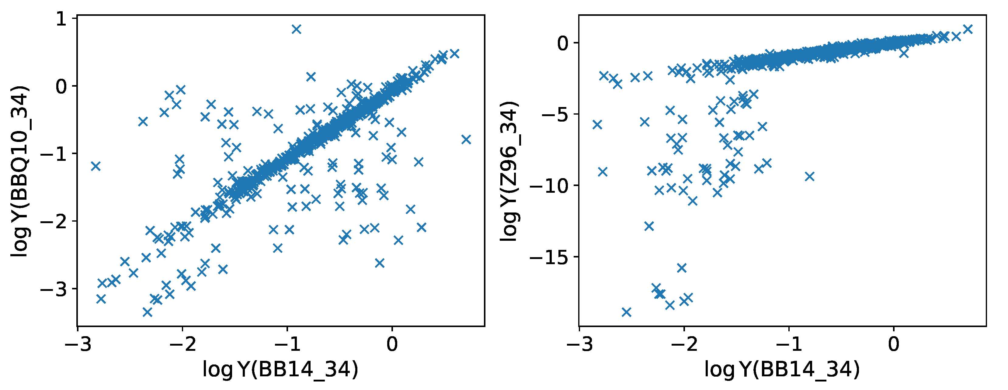
- atom_BBQ10_34, coll_BBQ10_34 —A-values and ECS were downloaded from the xstar database [57], and the PyNeb atom and coll files were rebuilt.
- atom_BB14_34, coll_BB14_34 —Computed A-values and ECS were obtained from the crlike_nrb13#fe2.dat adf04 file downloaded from the open-adas3 database. Details of the ECS computation [28] are described in Section 3.1. No information is given in the adf04 file on the provenance of the radiative data; thus, we assume they are coproducts of the target calculation.
- atom_BB14_144, coll_BB14_144 —The BB14_34 model has been extended to include 144 levels from the , , and configurations with cm.
3.3. Fe iii Observational Benchmarks
3.3.1. A-Value Ratio Benchmark
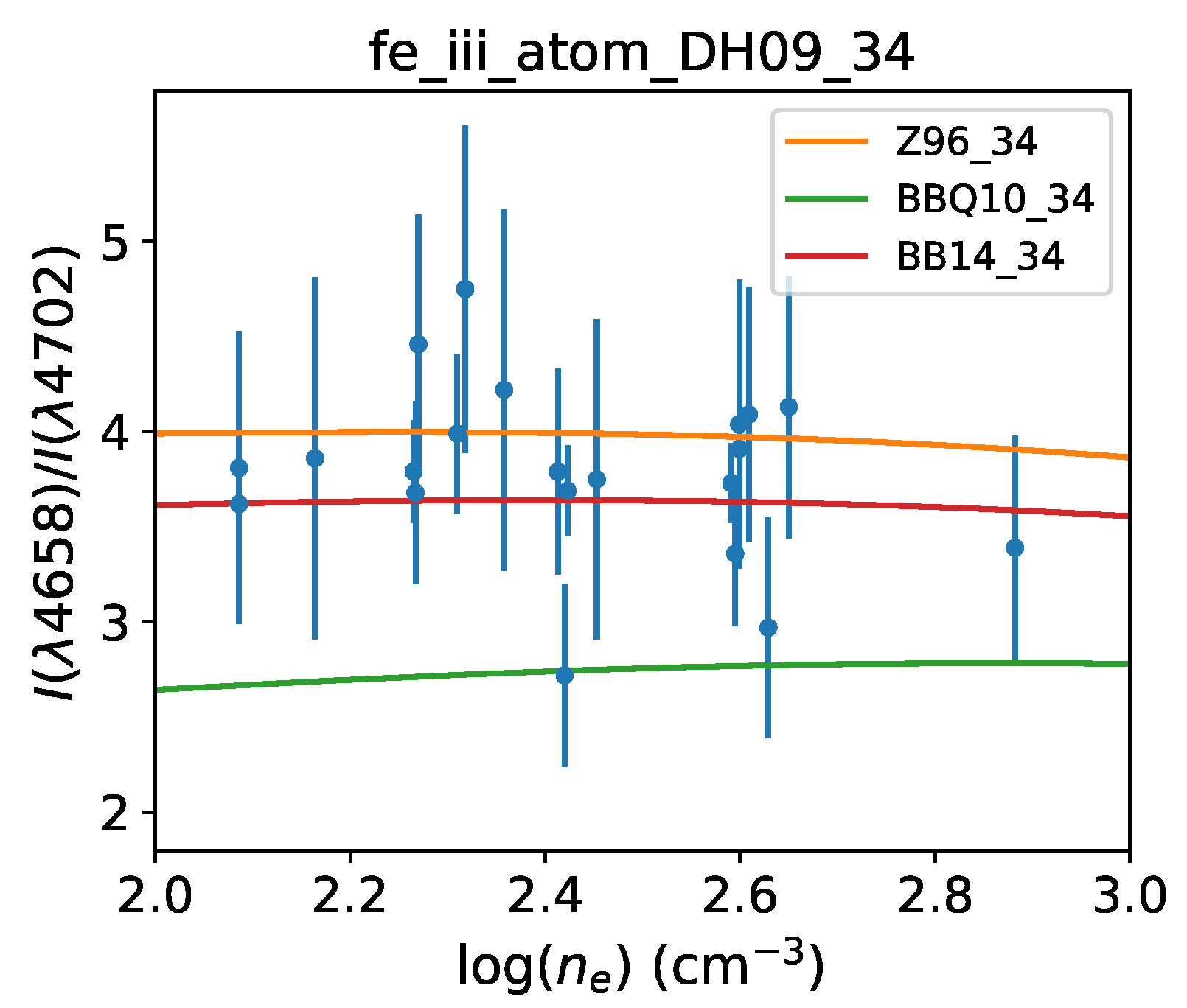
3.3.2. [Fe iii] Spectrum Fits
| # Call the PyNeb Python module import pyneb as pn # Select the radiative and collisional datasets pn.atomicData.setDataFile(’fe_iii_atom_Q96_J00.dat’) pn.atomicData.setDataFile(’fe_iii_coll_Z96.dat’) # Instantiate Fe III Fe3=pn.Atom(’Fe’,3) # Check the datafiles print(Fe3) # Determine and print the two emissivities e1=Fe3.getEmissivity(tem=1.e4,den=1.0e4,wave=5270.57) e2=Fe3.getEmissivity(tem=1.e4,den=1.0e4,lev_i=6,lev_j=2) print(e1,e2) |
- Misidentifications: , 9204
- Line blending or telluric contamination [9]: , 4931, 4987, 8729, 8838
- Small A-values ( s): , 4047.
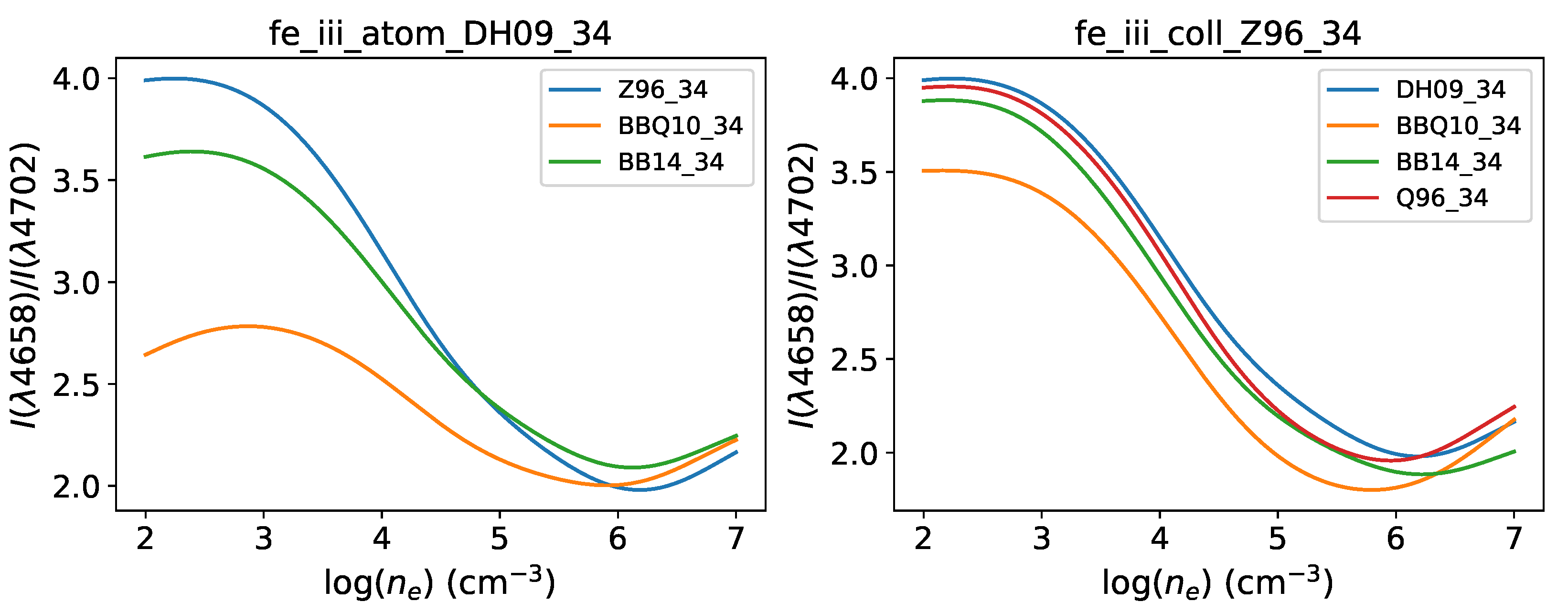
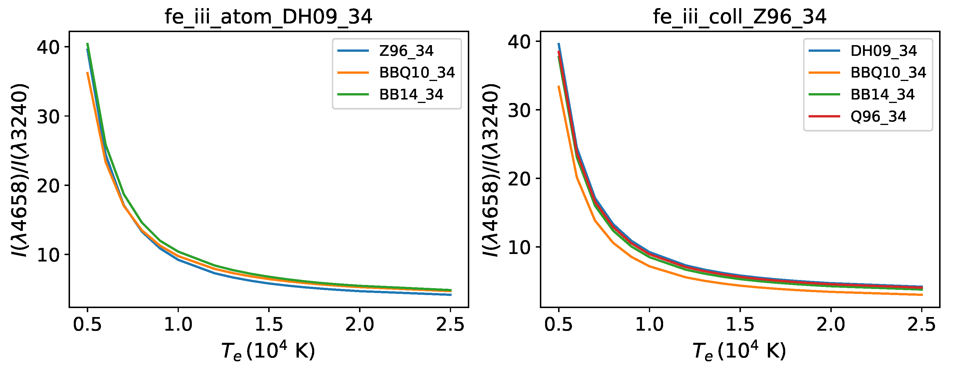
3.3.3. Line-Ratio Diagnostics
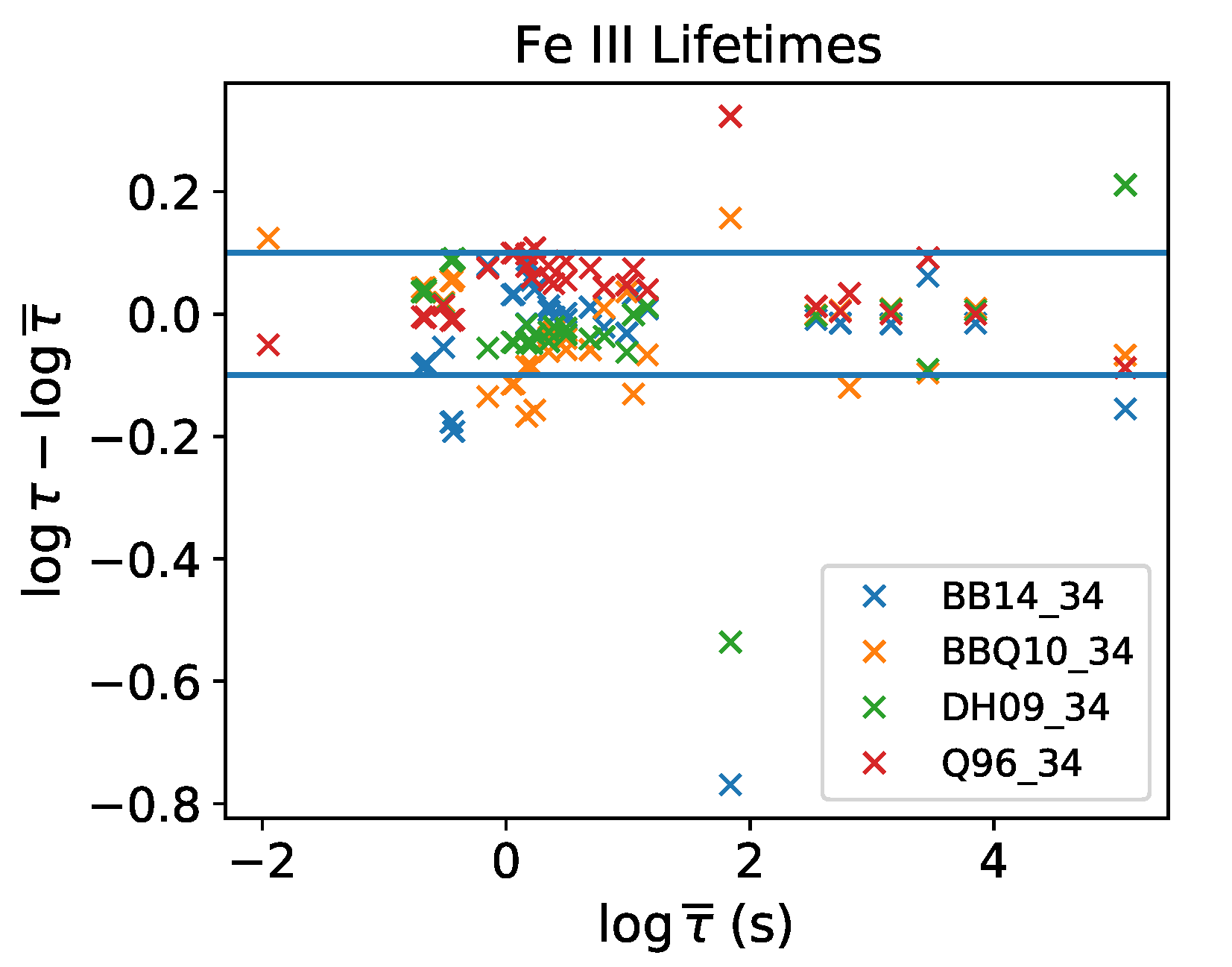
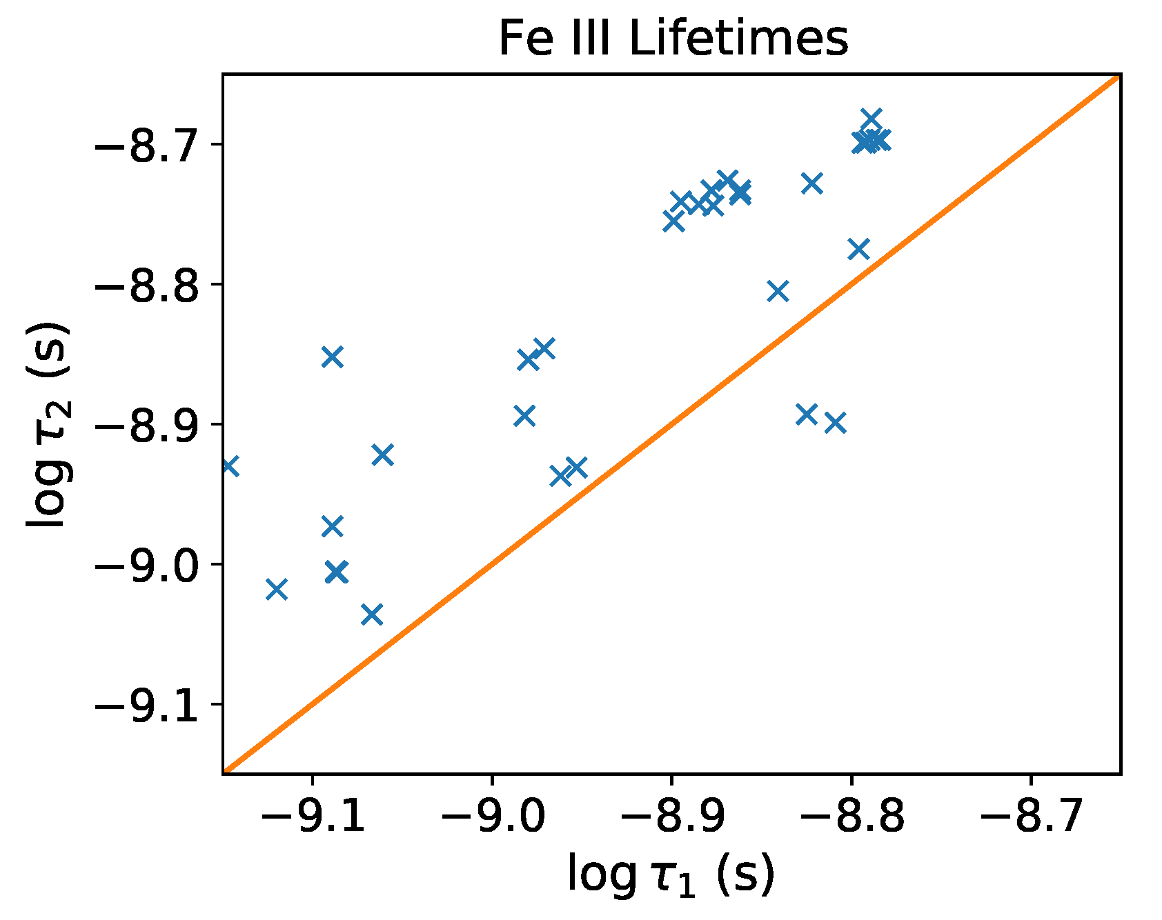
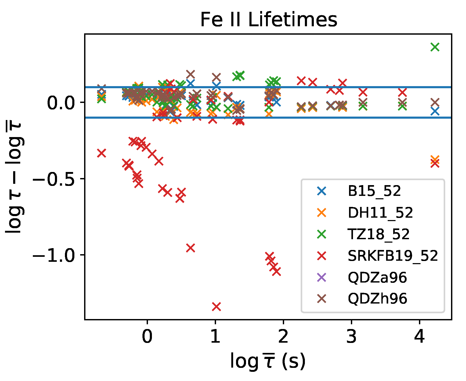
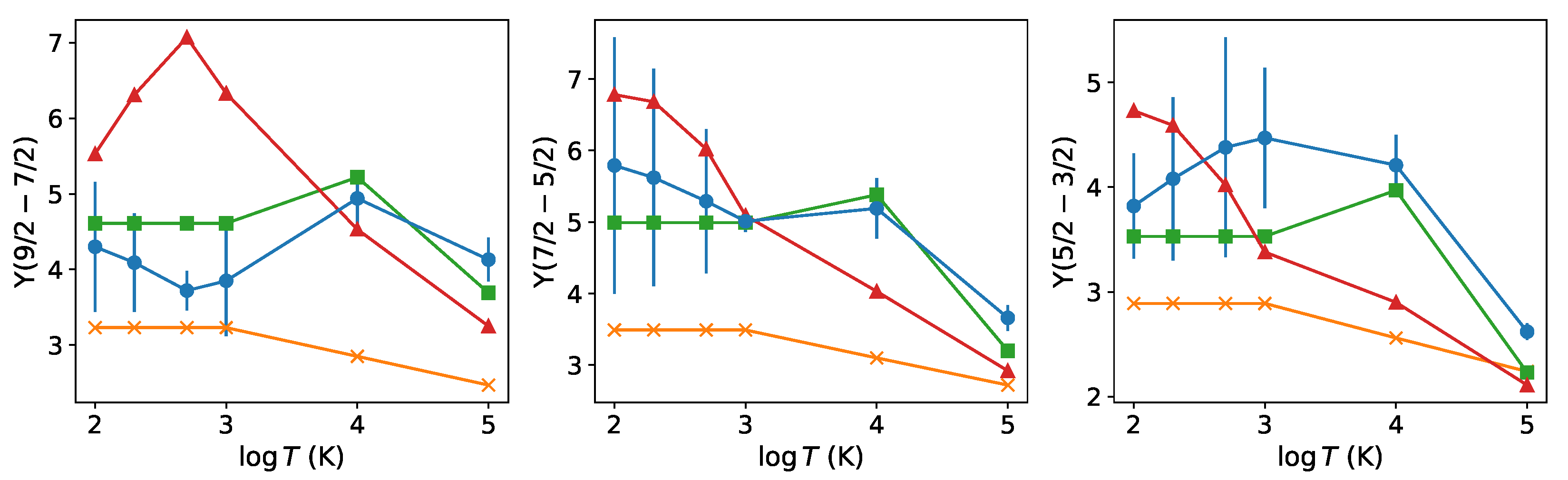
3.4. Radiative Lifetimes of and Levels
3.5. Radiative Lifetimes of Levels
3.6. Effective Collision Strengths
3.7. Fe iii Discussion
4. Fe ii
4.1. Fe ii Atomic Datasets in PyNeb
- atom_VVKFHF99, coll_VVKFHF99 —These datasets list radiative and collisional rates for transitions among 80 levels with energies cm compiled from different sources [71]. A-values for the dipole allowed and forbidden transitions are from [21] and [23], respectively. ECS are mainly from [24]; however, the source data are not available and A-values and ECS for transitions with spin change have been obviated.
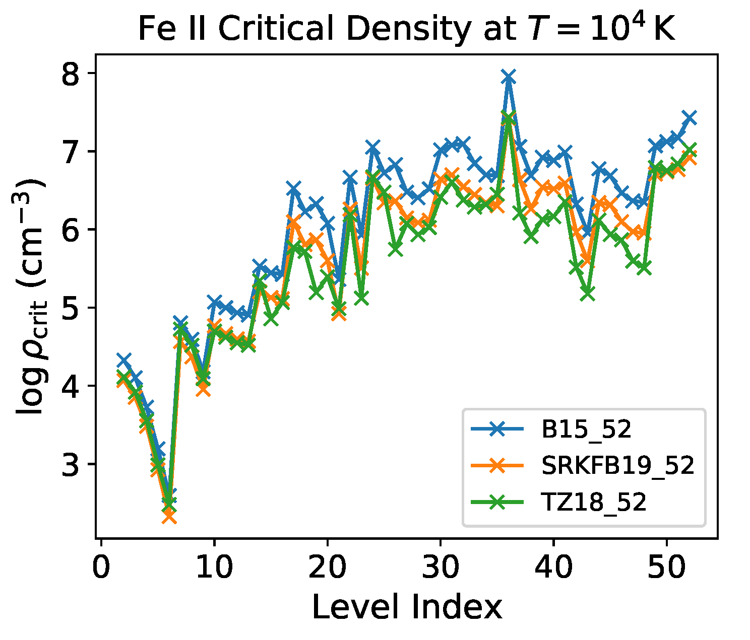
- atom_B15, coll_B15 —A-values and ECS for transitions among 52 levels belonging to the , , and configurations ( cm) [29]. A-values were computed with the mcbp atomic structure code autostructure using different expansions and orbital optimization strategies and a dipole correction to the Thomas–Fermi–Dirac–Amaldi potential. Fine-tuning was carried out by means of term-energy corrections adjusted by fitting to the experimental term energies. ECS were computed with the Dirac–Coulomb R-matrix package darc [34] using a target generated with the fully relativistic atomic structure code grasp0 [54] using a six-configuration expansion comprising 329 levels.
- atom_SRKFB19, coll_SRKFB19 —A-values and ECS for 250 levels from the , , , , and configurations [31]. A-values were computed with grasp0 in a 20-configuration expansion and ECS with darc using a 716-level target representation.
4.2. Fe ii Revised and New Atomic Datasets
- atom_QDZa96, atom_QDZh96 —E2 and M1 A-values calculated for transitions among the 63 levels of the configurations , , and [23]. Extensive CI expansion was used with the Breit–Pauli superstructure [18] (QDZa96) and Pauli hfr [20] (QDZh96) atomic structure codes. These datasets are not complete enough to be used in PyNeb spectral modeling as they obviate transitions such as and ; therefore, they will only be used in radiative data comparisons.
- atom_VVKFHF99_52, coll_VVKFHF99_52 —The VVKFHF99 datasets containing A-values and ECS described in Section 4.1 are reduced to 52 levels from even-parity configurations.
- atom_DH11_52 —E2 and M1 A-values for transitions between levels of the , , and configurations were computed in a large-scale CI framework with the mcbp structure code civ3 [42]. Wave functions were fine-tuned to fit the experimental energies.
- atom_B15_52, coll_B15_52 —Data (A-values and ECS) from the B15 calculation described in Section 4.1 were downloaded directly from the CDS, and the datasets were reconstructed.
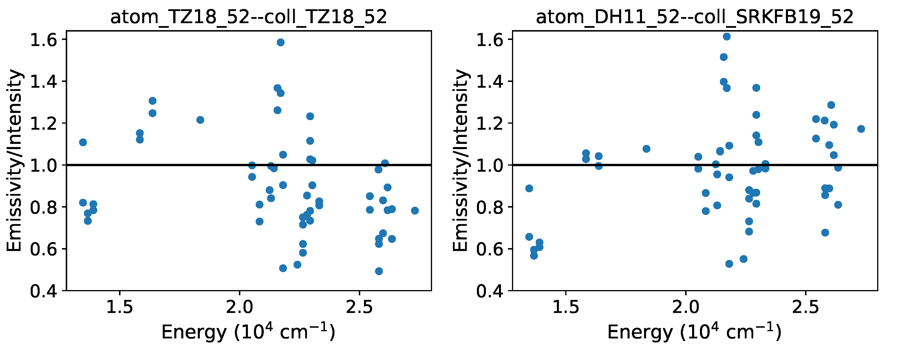
- atom_TZ18_52, coll_TZ18_52 —A-values and ECS were computed with the close-coupling B-spline Breit–Pauli R-matrix method for 340 levels of the , , , , and configurations [30]. The CI target representation was constructed with a Hartree–Fock method. Semi-empirical fine-tuning in the structure and scattering calculations was introduced by fitting tothe experimental energies. The final Hamiltonian of the scattering calculation contains the spin–orbit term.
- atom_SRKFB19_52, coll_SRKFB19_52 —Radiative and collisional data from the SRKFB19 calculation were described in Section 4.1. New files were constructed with data extracted from the adf04_DARC716_2.10.18 file (Cathy Ramsbottom, private communication) and reduced to 52 levels.
- atom_SRKFB19_173, coll_SRKFB19_173, atom_TZ18_173, coll_TZ18_173 —The SRKFB19 and TZ18 datasets have been extended to 173 levels ( cm) to test model convergence.
- atom_SRKFB19_225, atom_TZ18_225 —The theoretical SRKFB19 and TZ18 datasets have been extended to 225 levels ( cm) to bring out term assignment inconsistencies involving levels with total orbital angular momentum quantum number (see Table 6). With respect to NIST and other theoretical datasets, the term assignments of levels at and cm () and and cm () have been interchanged in atom_SRKFB19_225. Since the total angular momentum quantum number J of each level coincides in the different datasets, the incongruent term labeling would be inconsequential if the A-values for the transitions involving these levels were comparable. As shown in Table 7, this is not the case, as discrepancies as large as an order of magnitude were encountered. A similar mixup was found with the odd-parity and levels, which in this case are even energetically misplaced (see Table 6). Assignment discrepancies of this sort could be due to strong CI admixture in terms with high orbital angular momentum ( say) in lowly ionized systems that the grasp0 multi-configuration Dirac–Hartree–Fock structure code has problems resolving.
4.3. Observational and Spectroscopic Benchmarks
4.3.1. A-Value Ratio Benchmark
4.3.2. [Fe ii] Spectrum Fits
- coll_B15_52:
- coll_TZ18_52:
- coll_SRKFB19_52:
- coll_VVKFHF99_52:
- coll_B15_52:
- coll_TZ18_52:
- coll_SRKFB19_52:
- coll_VVKFHF99_52:
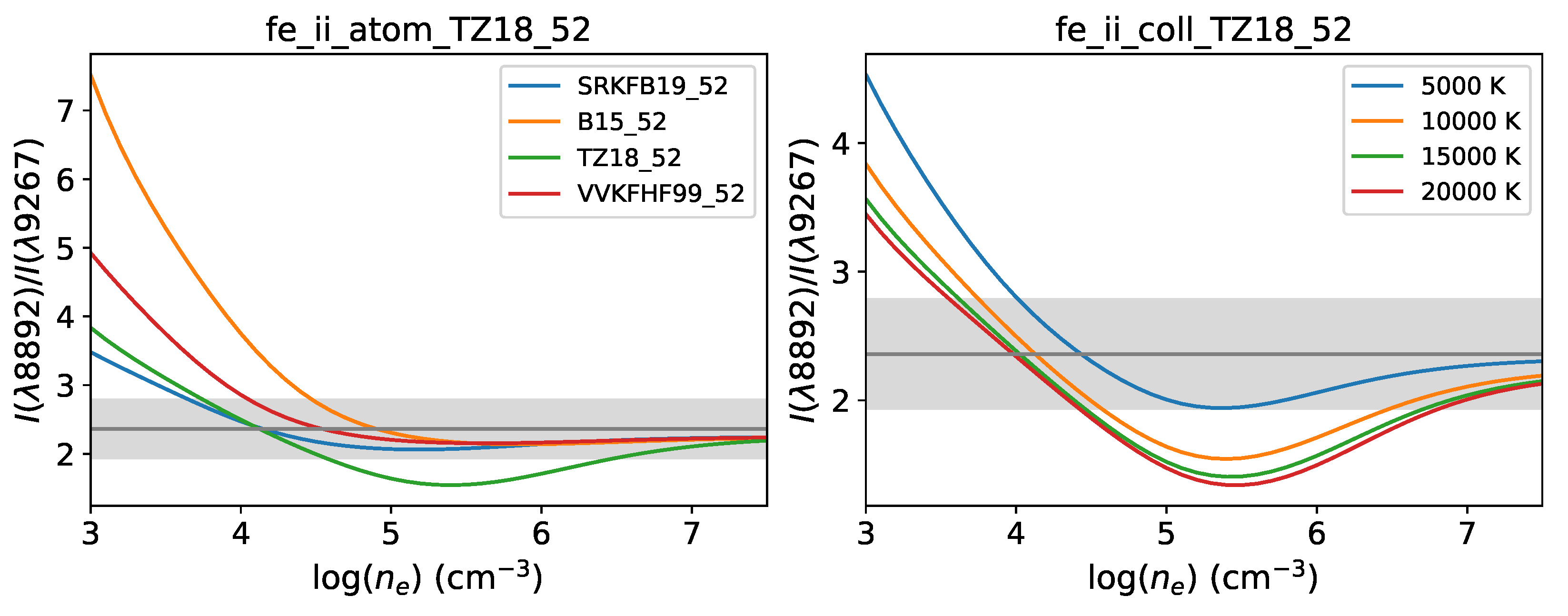
4.3.3. Line-Ratio Diagnostics
4.4. Radiative Lifetimes of the , , and Levels
4.5. Radiative Lifetimes of the Odd-Parity Levels
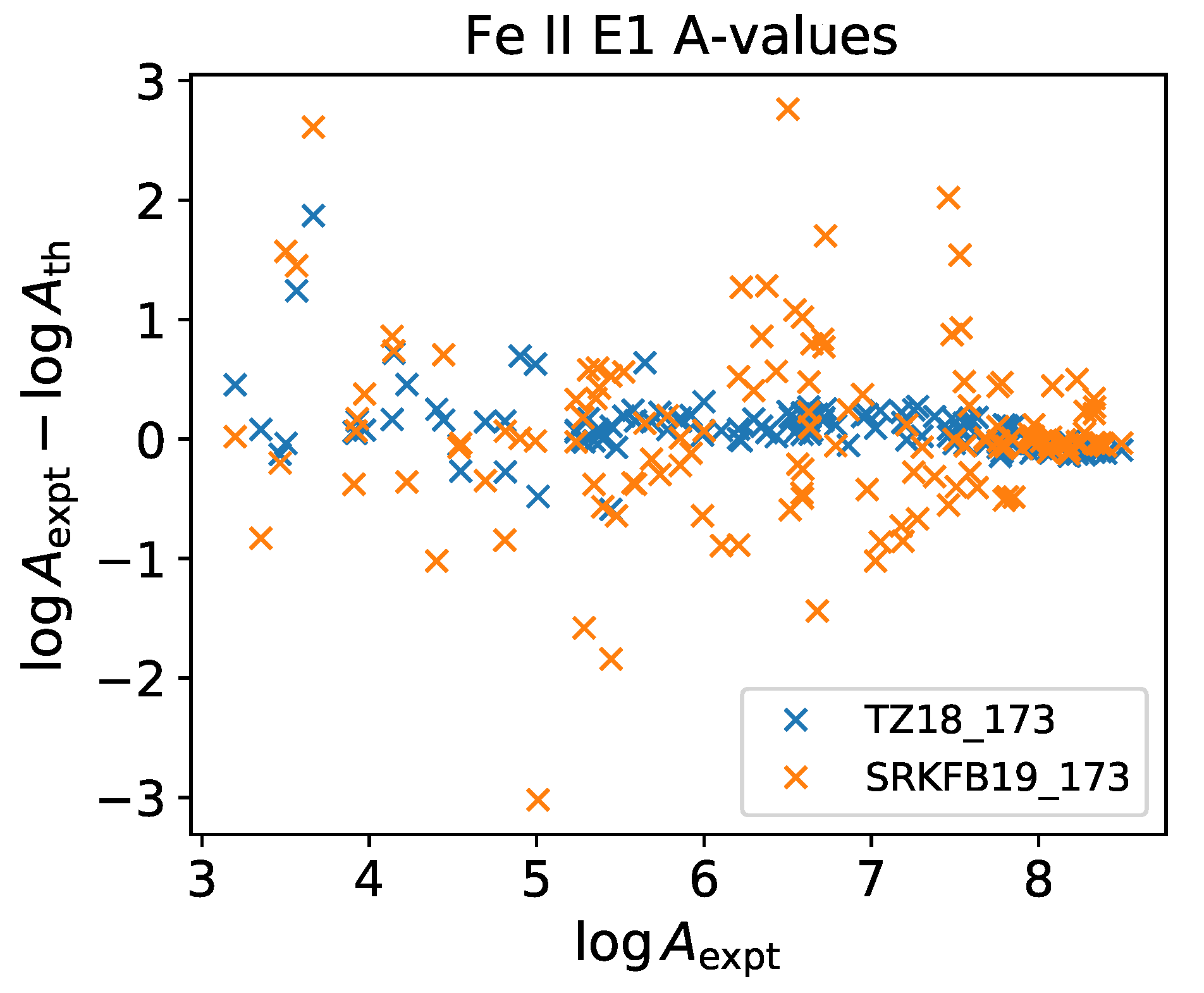
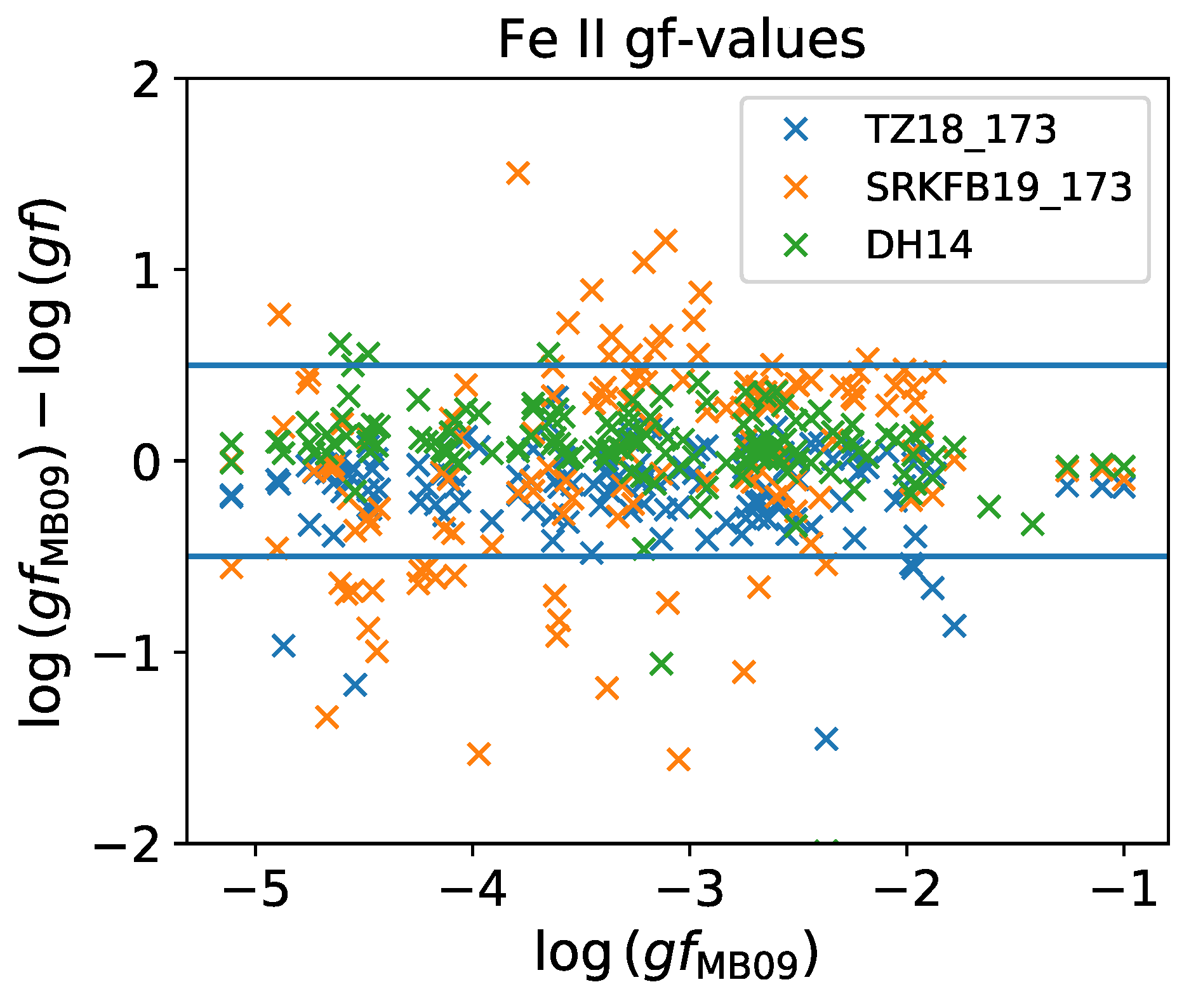
4.6. Fe ii -Values
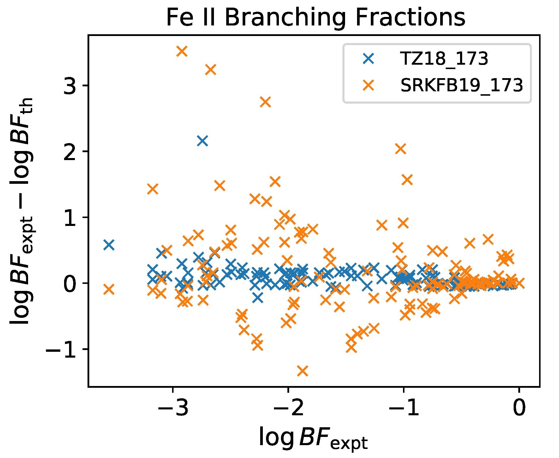
4.7. Fe ii Branching Fractions
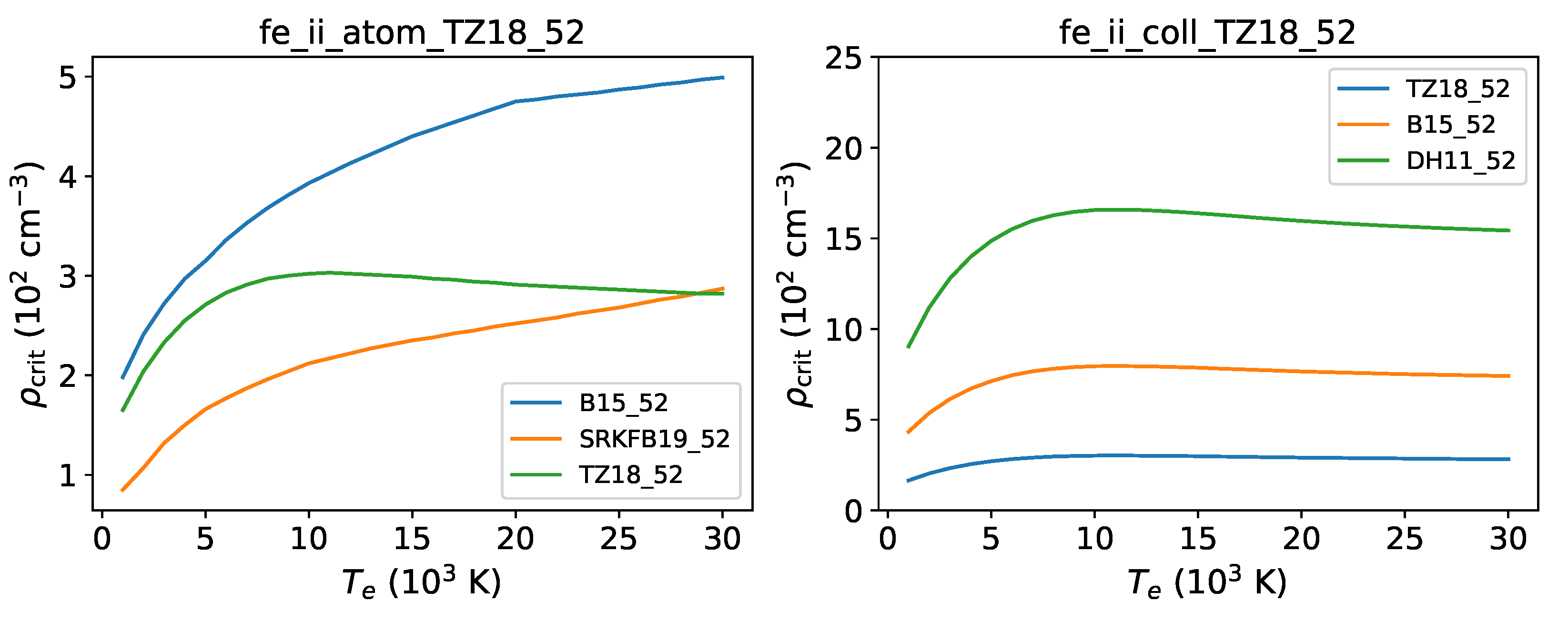
4.8. [Fe ii] Effective Collision Strengths
4.9. Fe ii Discussion
5. Conclusions
Author Contributions
Funding
Data Availability Statement
Acknowledgments
Conflicts of Interest
Abbreviations
| CDS | Centre de Données astronomiques de Strasbourg |
| NIST | National Institute os Standards and Technology |
Appendix A

| Fe iii File Name | v1.1.16 | v1.1.17 | Fe ii File Name | v1.1.16 | v1.1.17 |
|---|---|---|---|---|---|
| fe_iii_atom_BB14_144.dat | * | fe_ii_atom_TZ18_173.dat | * | ||
| fe_iii_atom_BBQ10.dat | X | X | fe_ii_atom_B15.dat | * | D |
| fe_iii_atom_DH09_34.dat | X | fe_ii_atom_B15_52.dat | X | ||
| fe_iii_atom_NP96.dat | X | X | fe_ii_atom_DH11_52.dat | X | |
| fe_iii_atom_Q96_34.dat | X | fe_ii_atom_SRKFB19.dat | X | D | |
| fe_iii_atom_Q96_J00.dat | * | X | fe_ii_atom_VVKFHF99.dat | X | D |
| fe_iii_coll_BB14_144.dat | * | fe_ii_coll_TZ18_173.dat | * | ||
| fe_iii_coll_BB14.dat | X | D | fe_ii_coll_B15.dat | * | D |
| fe_iii_coll_BBQ10.dat | X | D | fe_ii_coll_B15_52.dat | X | |
| fe_iii_coll_BBQ10_34.dat | X | fe_ii_coll_B15_old.dat | X | D | |
| fe_iii_coll_Q96.dat | X | X | fe_ii_coll_SRKFB19.dat | X | X |
| fe_iii_coll_Z96.dat | * | X | fe_ii_coll_VVKFHF99.dat | X | D |
| fe_iii_coll_Z96_144.dat | X |
| 1 | |
| 2 | |
| 3 |
References
- Luridiana, V.; Morisset, C.; Shaw, R.A. PyNeb: A New Software for the Analysis of Emission Lines. In IAU Symposium; Cambridge University Press: Cambridge, UK, 2012; Volume 283, pp. 422–423. [Google Scholar] [CrossRef] [Green Version]
- Luridiana, V.; Morisset, C.; Shaw, R.A. PyNeb: A new tool for analyzing emission lines. I. Code description and validation of results. Astron. Astrophys. 2015, 573, A42. [Google Scholar] [CrossRef] [Green Version]
- Peimbert, M.; Peimbert, A.; Delgado-Inglada, G. Nebular Spectroscopy: A Guide on H II Regions and Planetary Nebulae. Publ. Astron. Soc. Pac. 2017, 129, 082001. [Google Scholar] [CrossRef]
- Morisset, C.; Luridiana, V.; García-Rojas, J.; Gómez-Llanos, V.; Bautista, M.; Mendoza, C. Atomic Data Assessment with PyNeb. Atoms 2020, 8, 66. [Google Scholar] [CrossRef]
- Juan de Dios, L.; Rodríguez, M. Atomic data and the density structures of planetary nebulae. Mon. Not. R. Astron. Soc. 2021, 507, 5331–5339. [Google Scholar] [CrossRef]
- Perinotto, M.; Bencini, C.G.; Pasquali, A.; Manchado, A.; Rodriguez Espinosa, J.M.; Stanga, R. The iron abundance in four planetary nebulae. Astron. Astrophys. 1999, 347, 967–974. [Google Scholar]
- Delgado Inglada, G.; Rodríguez, M.; Mampaso, A.; Viironen, K. The Iron Abundance in Galactic Planetary Nebulae. Astrophys. J. 2009, 694, 1335–1348. [Google Scholar] [CrossRef]
- Delgado-Inglada, G.; Mesa-Delgado, A.; García-Rojas, J.; Rodríguez, M.; Esteban, C. The Fe/Ni ratio in ionized nebulae: Clues on dust depletion patterns. Mon. Not. R. Astron. Soc. 2016, 456, 3855–3865. [Google Scholar] [CrossRef] [Green Version]
- Mesa-Delgado, A.; Esteban, C.; García-Rojas, J.; Luridiana, V.; Bautista, M.; Rodríguez, M.; López-Martín, L.; Peimbert, M. Properties of the ionized gas in HH 202—II. Results from echelle spectrophotometry with Ultraviolet Visual Echelle Spectrograph. Mon. Not. R. Astron. Soc. 2009, 395, 855–876. [Google Scholar] [CrossRef]
- Méndez-Delgado, J.E.; Esteban, C.; García-Rojas, J.; Henney, W.J.; Mesa-Delgado, A.; Arellano-Córdova, K.Z. Photoionized Herbig-Haro objects in the Orion Nebula through deep high-spectral resolution spectroscopy—I. HH 529 II and III. Mon. Not. R. Astron. Soc. 2021, 502, 1703–1739. [Google Scholar] [CrossRef]
- Méndez-Delgado, J.E.; Henney, W.J.; Esteban, C.; García-Rojas, J.; Mesa-Delgado, A.; Arellano-Córdova, K.Z. Photoionized Herbig-Haro Objects in the Orion Nebula through Deep High Spectral Resolution Spectroscopy. II. HH 204. Astrophys J. 2021, 918, 27. [Google Scholar] [CrossRef]
- D’Odorico, S.; Cristiani, S.; Dekker, H.; Hill, V.; Kaufer, A.; Kim, T.; Primas, F. Performance of UVES, the echelle spectrograph for the ESO VLT and highlights of the first observations of stars and quasars. In Discoveries and Research Prospects from 8- to 10-Meter-Class Telescopes; Bergeron, J., Ed.; Society of Photo-Optical Instrumentation Engineers (SPIE): Bellingham, WA, USA, 2000; Volume 4005, pp. 121–130. [Google Scholar] [CrossRef]
- Garstang, R.H. Transition probabilities for forbidden lines of Fe II. Mon. Not. R. Astron. Soc. 1962, 124, 321. [Google Scholar] [CrossRef]
- Kurucz, R.L.; Peytremann, E. A Table of Semiempirical gf Values. Pt 1: Wavelengths: 5.2682 NM to 272.3380 nm; Pt 2: Wavelengths: 272.3395 NM to 599.3892 nm; Pt 3: Wavelengths: 599.4004 NM to 9997.2746 NM; SAO Special Report; Smithsonian Astrophysical Observatory: Cambridge, MA, USA, 1975. [Google Scholar]
- Nussbaumer, H.; Storey, P.J. Atomic data for Fe II. Astron. Astrophys. 1980, 89, 308–313. [Google Scholar]
- Nussbaumer, H.; Pettini, M.; Storey, P.J. Sextet transitions in Fe II. Astron. Astrophys. 1981, 102, 351–358. [Google Scholar]
- Hummer, D.G.; Berrington, K.A.; Eissner, W.; Pradhan, A.K.; Saraph, H.E.; Tully, J.A. Atomic data from the IRON project. I. Goals and methods. Astron. Astrophys 1993, 279, 298–309. [Google Scholar]
- Eissner, W.; Jones, M.; Nussbaumer, H. Techniques for the calculation of atomic structures and radiative data including relativistic corrections. Comput. Phys. Commun. 1974, 8, 270–306. [Google Scholar] [CrossRef]
- Hibbert, A. CIV3—A general program to calculate configuration interaction wave functions and electric-dipole oscillator strengths. Comput. Phys. Commun. 1975, 9, 141–172. [Google Scholar] [CrossRef]
- Cowan, R.D. The Theory of Atomic Structure and Spectra; University of California: Berkeley, CA, USA, 1981. [Google Scholar]
- Nahar, S.N. Atomic data from the Iron Project. VII. Radiative dipole transition probabilities for Fe II. Astron. Astrophys. 1995, 293, 967–977. [Google Scholar]
- Nahar, S.N.; Pradhan, A.K. Atomic data from the Iron Project. XVII. Radiative transition probabilities for dipole allowed and forbidden transitions in Fe III. Astron. Astrophys. Suppl. Ser. 1996, 119, 509–522. [Google Scholar] [CrossRef]
- Quinet, P.; Le Dourneuf, M.; Zeippen, C.J. Atomic data from the IRON Project. XIX. Radiative transition probabilities for forbidden lines in Fe II. Astron. Astrophys. Suppl. Ser. 1996, 120, 361–371. [Google Scholar] [CrossRef]
- Zhang, H.L.; Pradhan, A.K. Atomic data from the Iron Project. VI. Collision strengths and rate coefficients for Fe II. Astron. Astrophys. 1995, 293, 953–966. [Google Scholar]
- Zhang, H. Atomic data from the Iron Project. XVIII. Electron impact excitation collision strengths and rate coefficients for Fe III. Astron. Astrophys. Suppl. Ser. 1996, 119, 523–528. [Google Scholar] [CrossRef]
- Bautista, M.A.; Pradhan, A.K. Atomic data from the Iron project. XIII. Electron excitation rates and emissivity ratios for forbidden transitions in Ni II and Fe II. Astron. Astrophys. Suppl. Ser. 1996, 115, 551–559. [Google Scholar]
- Bautista, M.A.; Ballance, C.P.; Quinet, P. Atomic Data and Spectral Model for Fe III. Astrophys. J. 2010, 718, L189–L193. [Google Scholar] [CrossRef] [Green Version]
- Badnell, N.R.; Ballance, C.P. Electron-impact Excitation of Fe2+: A Comparison of Intermediate Coupling Frame Transformation, Breit-Pauli and Dirac R-matrix Calculations. Astrophys. J. 2014, 785, 99. [Google Scholar] [CrossRef] [Green Version]
- Bautista, M.A.; Fivet, V.; Ballance, C.; Quinet, P.; Ferland, G.; Mendoza, C.; Kallman, T.R. Atomic Data and Spectral Model for Fe II. Astrophys. J. 2015, 808, 174. [Google Scholar] [CrossRef] [Green Version]
- Tayal, S.S.; Zatsarinny, O. Electron-impact excitation of forbidden and allowed transitions in Fe II. Phys. Rev. A 2018, 98, 012706. [Google Scholar] [CrossRef] [Green Version]
- Smyth, R.T.; Ramsbottom, C.A.; Keenan, F.P.; Ferland, G.J.; Ballance, C.P. Towards converged electron-impact excitation calculations of low-lying transitions in Fe II. Mon. Not. R. Astron. Soc. 2019, 483, 654–663. [Google Scholar] [CrossRef] [Green Version]
- Berrington, K.A.; Eissner, W.B.; Norrington, P.H. RMATRX1: Belfast atomic R-matrix codes. Comput. Phys. Commun. 1995, 92, 290–420. [Google Scholar] [CrossRef]
- Zatsarinny, O. BSR: B-spline atomic R-matrix codes. Comput. Phys. Commun. 2006, 174, 273–356. [Google Scholar] [CrossRef]
- Ait-Tahar, S.; Grant, I.P.; Norrington, P.H. Electron scattering by Fe XXII within the Dirac R-matrix approach. Phys. Rev. A 1996, 54, 3984–3989. [Google Scholar] [CrossRef]
- Griffin, D.C.; Badnell, N.R.; Pindzola, M.S. R-matrix electron-impact excitation cross sections in intermediate coupling: An MQDT transformation approach. J. Phys. B At. Mol. Phys. 1998, 31, 3713–3727. [Google Scholar] [CrossRef]
- Wan, Y.; Favreau, C.; Loch, S.D.; McLaughlin, B.M.; Qi, Y.; Stancil, P.C. Electron-impact fine-structure excitation of Fe II at low temperature. Mon. Not. R. Astron. Soc. 2019, 485, 2252–2258. [Google Scholar] [CrossRef]
- Deb, N.C.; Hibbert, A. Oscillator strengths for transitions among Fe III levels belonging to the three lowest configurations. J. Phys. Conf. Ser. 2008, 130, 012006. [Google Scholar] [CrossRef] [Green Version]
- Deb, N.C.; Hibbert, A. Electric quadrupole and magnetic dipole transitions among 3d6 levels of Fe III. J. Phys. B Atom. Mol. Phys. 2009, 42, 065003. [Google Scholar] [CrossRef]
- Deb, N.C.; Hibbert, A. Weighted f-values, A-values, and line strengths for the E1 transitions among 3d 6, 3d 54s, and 3d 54p levels of Fe III. Atom. Data Nucl. Data Tables. 2009, 95, 184–303. [Google Scholar] [CrossRef]
- Deb, N.C.; Hibbert, A. Importance of level mixing on accurate [Fe II] transition rates. Astron. Astrophys. 2010, 524, A54. [Google Scholar] [CrossRef] [Green Version]
- Deb, N.C.; Hibbert, A. Calculation of Intensity Ratios of Observed Infrared [Fe II] Lines. Astrophys. J. 2010, 711, L104–L107. [Google Scholar] [CrossRef]
- Deb, N.C.; Hibbert, A. Radiative transition rates for the forbidden lines in Fe II. Astron. Astrophys. 2011, 536, A74. [Google Scholar] [CrossRef] [Green Version]
- Deb, N.C.; Hibbert, A. log gf values for astrophysically important transitions Fe II. Astron. Astrophys. 2014, 561, A32. [Google Scholar] [CrossRef] [Green Version]
- Quinet, P. Transition probabilities for forbidden lines of Fe III. Astron. Astrophys. Suppl. Ser. 1996, 116, 573–578. [Google Scholar] [CrossRef] [Green Version]
- Fivet, V.; Quinet, P.; Bautista, M.A. Radiative rates for forbidden M1 and E2 transitions of astrophysical interest in doubly ionized iron-peak elements. Astron. Astrophys 2016, 585, A121. [Google Scholar] [CrossRef] [Green Version]
- Schnabel, R.; Schultz-Johanning, M.; Kock, M. Fe II lifetimes and transition probabilities. Astron. Astrophys. 2004, 414, 1169–1176. [Google Scholar] [CrossRef] [Green Version]
- Meléndez, J.; Barbuy, B. Both accurate and precise gf-values for Fe II lines. Astron. Astrophys. 2009, 497, 611–617. [Google Scholar] [CrossRef] [Green Version]
- Den Hartog, E.A.; Lawler, J.E.; Sneden, C.; Cowan, J.J.; Brukhovesky, A. Atomic Transition Probabilities for UV and Blue Lines of Fe II and Abundance Determinations in the Photospheres of the Sun and Metal-poor Star HD 84937. Astrophys. J. Suppl, Ser. 2019, 243, 33. [Google Scholar] [CrossRef] [Green Version]
- Rostohar, D.; Derkatch, A.; Hartman, H.; Johansson, S.; Lundberg, H.; Mannervik, S.; Norlin, L.O.; Royen, P.; Schmitt, A. Lifetime Measurements of Metastable States in Fe+. Phys. Rev. Lett. 2001, 86, 1466–1469. [Google Scholar] [CrossRef] [Green Version]
- Hartman, H.; Derkatch, A.; Donnelly, M.P.; Gull, T.; Hibbert, A.; Johansson, S.; Lundberg, H.; Mannervik, S.; Norlin, L.O.; Rostohar, D.; et al. The FERRUM Project: Experimental transition probabilities of [Fe II] and astrophysical applications. Astron. Astrophys. 2003, 397, 1143–1149. [Google Scholar] [CrossRef] [Green Version]
- Gurell, J.; Hartman, H.; Blackwell-Whitehead, R.; Nilsson, H.; Bäckström, E.; Norlin, L.O.; Royen, P.; Mannervik, S. The FERRUM project: Transition probabilities for forbidden lines in [Fe II] and experimental metastable lifetimes. Astron. Astrophys. 2009, 508, 525–529. [Google Scholar] [CrossRef] [Green Version]
- Johansson, S.; Zethson, T.; Hartman, H.; Ekberg, J.O.; Ishibashi, K.; Davidson, K.; Gull, T. New forbidden and fluorescent Fe III lines identified in HST spectra of eta Carinae. Astron. Astrophys. 2000, 361, 977–981. [Google Scholar]
- Badnell, N.R. A Breit-Pauli distorted wave implementation for AUTOSTRUCTURE. Comput. Phys. Commun. 2011, 182, 1528–1535. [Google Scholar] [CrossRef]
- Parpia, F.A.; Fischer, C.F.; Grant, I.P. GRASP92: A package for large-scale relativistic atomic structure calculations. Comput. Phys. Commun. 1996, 94, 249–271. [Google Scholar] [CrossRef]
- Kramida, A.; Yu, R.; Reader, J.; NIST ASD Team. NIST Atomic Spectra Database, version 5.9; Reader, J., Ed.; National Institute of Standards and Technology: Gaithersburg, MD, USA, 2021. [Google Scholar]
- Hibbert, A.; Glass, R.; Froese Fischer, C. A general program for computing angular integrals of the Breit-Pauli Hamiltonian. Comput. Phys. Commun. 1991, 64, 455–472. [Google Scholar] [CrossRef]
- Mendoza, C.; Bautista, M.A.; Deprince, J.; García, J.A.; Gatuzz, E.; Gorczyca, T.W.; Kallman, T.R.; Palmeri, P.; Quinet, P.; Witthoeft, M.C. The XSTAR Atomic Database. Atoms 2021, 9, 12. [Google Scholar] [CrossRef]
- Storey, P.J.; Sochi, T. Electron temperatures and free-electron energy distributions of nebulae from C II dielectronic recombination lines. Mon. Not. R. Astron. Soc. 2013, 430, 599–610. [Google Scholar] [CrossRef]
- Sochi, T. Atomic and Molecular Aspects of Astronomical Spectra. Ph.D. Thesis, University College, London, UK, 2012. [Google Scholar]
- Peimbert, A. The Chemical Composition of the 30 Doradus Nebula Derived from Very Large Telescope Echelle Spectrophotometry. Astrophys. J. 2003, 584, 735–750. [Google Scholar] [CrossRef] [Green Version]
- García-Rojas, J.; Esteban, C.; Peimbert, A.; Peimbert, M.; Rodríguez, M.; Ruiz, M.T. Deep echelle spectrophotometry of S 311, a Galactic HII region located outside the solar circle. Mon. Not. R. Astron. Soc. 2005, 362, 301–312. [Google Scholar] [CrossRef] [Green Version]
- García-Rojas, J.; Esteban, C.; Peimbert, M.; Costado, M.T.; Rodríguez, M.; Peimbert, A.; Ruiz, M.T. Faint emission lines in the Galactic H II regions M16, M20 and NGC 3603. Mon. Not. R. Astron. Soc. 2006, 368, 253–279. [Google Scholar] [CrossRef] [Green Version]
- García-Rojas, J.; Esteban, C.; Peimbert, A.; Rodríguez, M.; Peimbert, M.; Ruiz, M.T. The chemical composition of the Galactic H II regions M8 and M17. A revision based on deep VLT echelle spectrophotometry. Rev. Mex. Astron. Astrofis. 2007, 43, 3–31. [Google Scholar]
- López-Sánchez, Á.R.; Esteban, C.; García-Rojas, J.; Peimbert, M.; Rodríguez, M. The Localized Chemical Pollution in NGC 5253 Revisited: Results from Deep Echelle Spectrophotometry. Astrophys. J. 2007, 656, 168–185. [Google Scholar] [CrossRef]
- Esteban, C.; Bresolin, F.; Peimbert, M.; García-Rojas, J.; Peimbert, A.; Mesa-Delgado, A. Keck HIRES Spectroscopy of Extragalactic H II Regions: C and O Abundances from Recombination Lines. Astrophys. J. 2009, 700, 654–678. [Google Scholar] [CrossRef]
- Esteban, C.; García-Rojas, J.; Carigi, L.; Peimbert, M.; Bresolin, F.; López-Sánchez, A.R.; Mesa-Delgado, A. Carbon and oxygen abundances from recombination lines in low-metallicity star-forming galaxies. Implications for chemical evolution. Mon. Not. R. Astron. Soc. 2014, 443, 624–647. [Google Scholar] [CrossRef] [Green Version]
- Esteban, C.; Fang, X.; García-Rojas, J.; Toribio San Cipriano, L. The radial abundance gradient of oxygen towards the Galactic anti-centre. Mon. Not. R. Astron. Soc. 2017, 471, 987–1004. [Google Scholar] [CrossRef] [Green Version]
- Esteban, C.; Bresolin, F.; García-Rojas, J.; Toribio San Cipriano, L. Carbon, nitrogen, and oxygen abundance gradients in M101 and M31. Mon. Not. R. Astron. Soc. 2020, 491, 2137–2155. [Google Scholar] [CrossRef]
- Esteban, C.; García-Rojas, J. Revisiting the radial abundance gradients of nitrogen and oxygen of the Milky Way. Mon. Not. R. Astron. Soc. 2018, 478, 2315–2336. [Google Scholar] [CrossRef]
- Domínguez-Guzmán, G.; Rodríguez, M.; García-Rojas, J.; Esteban, C.; Toribio San Cipriano, L. The homogeneity of chemical abundances in H II regions of the Magellanic Clouds. Mon. Not. R. Astron. Soc. 2022, 517, 4497–4514. [Google Scholar] [CrossRef]
- Verner, E.M.; Verner, D.A.; Korista, K.T.; Ferguson, J.W.; Hamann, F.; Ferland, G.J. Numerical Simulations of Fe II Emission Spectra. Astrophys. J. Suppl. Ser. 1999, 120, 101–112. [Google Scholar] [CrossRef] [Green Version]
- Rodríguez, M. Fluorescence of [Fe II] in H II regions. Astron. Astrophys. 1999, 348, 222–226. [Google Scholar]
- Verner, E.M.; Verner, D.A.; Baldwin, J.A.; Ferland, G.J.; Martin, P.G. Continuum Pumping of [Fe II] in the Orion Nebula. Astrophys. J. 2000, 543, 831–839. [Google Scholar] [CrossRef]
- Hartman, H. Fluorescence in Astrophysical Plasmas. In New Trends in Atomic and Molecular Physics; Springer: Berlin/Heidelberg, Germany, 2013; p. 189. [Google Scholar] [CrossRef] [Green Version]
- Sarkar, A.; Ferland, G.J.; Chatzikos, M.; Guzmán, F.; van Hoof, P.A.M.; Smyth, R.T.; Ramsbottom, C.A.; Keenan, F.P.; Ballance, C.P. Improved Fe II Emission-line Models for AGNs Using New Atomic Data Sets. Astrophys. J. 2021, 907, 12. [Google Scholar] [CrossRef]


| J | (Å) | A-Value (s) | ||||
|---|---|---|---|---|---|---|
| J00 | BBQ10_34 | BB14_34 | FBQh16 | FBQa16 | ||
| 4 | 2438.28 | 22.2 | 25.7 | 38.4 | 32.0 | 31.6 |
| 3 | 2464.48 | 16.0 | 18.7 | 28.0 | 23.3 | 23.1 |
| 2 | 2483.01 | 11.0 | 12.8 | 19.1 | 15.9 | 15.8 |
| 1 | 2495.01 | 6.4 | 7.43 | 11.1 | 9.29 | 9.22 |
| 0 | 2500.93 | 2.0 | 2.44 | 3.66 | ||
| Line 1 | Line 2 | Obs | BBQ10_34 | BB14_34 | DH09_34 | Q96_34 | |||
|---|---|---|---|---|---|---|---|---|---|
| Upper | Lower | (Å) | Lower | (Å) | Line Intensity Ratio | ||||
| 3239.79 | 3286.24 | 4(1) | 3.58 | 3.59 | 3.28 | 3.60 | |||
| 3286.24 | 8728.84 | 2.0(5) | 4.88 | 3.12 | 3.80 | 3.29 | |||
| 3355.50 | 3366.22 | 1.6(8) | 1.13 | 1.12 | 1.16 | 1.14 | |||
| 3366.22 | 9959.85 | 5(4) | 9.07 | 5.42 | 6.37 | 5.54 | |||
| 3334.95 | 3356.59 | 1.2(2) | 1.14 | 1.15 | 1.20 | 1.18 | |||
| 3356.59 | 8838.14 | 4.1(8) | 6.01 | 4.28 | 4.39 | 4.19 | |||
| 3322.47 | 3371.35 | 1.4(3) | 1.38 | 1.37 | |||||
| 3371.35 | 3406.11 | 2.2(5) | 2.33 | 2.31 | |||||
| 4046.49 | 4096.68 | 2.3(8) | 2.27 | 2.45 | 2.56 | 2.53 | |||
| 4008.34 | 4079.69 | 3.8(7) | 3.15 | 3.63 | 3.62 | 3.92 | |||
| 4667.11 | 4734.00 | 0.29(4) | 0.28 | 0.28 | 0.29 | 0.28 | |||
| 4734.00 | 4777.70 | 2.0(3) | 2.06 | 2.07 | 2.09 | 2.08 | |||
| 4607.12 | 4701.64 | 0.19(3) | 0.18 | 0.18 | 0.19 | 0.17 | |||
| 4701.64 | 4769.53 | 2.8(3) | 2.89 | 2.90 | 2.93 | 2.94 | |||
| 4658.17 | 4754.81 | 5.3(6) | 5.28 | 5.40 | 5.32 | 5.49 | |||
| 5011.41 | 5084.85 | 5.9(9) | 5.72 | 6.12 | 5.97 | 5.95 | |||
| 4881.07 | 4987.29 | 5.4(7) | 4.99 | 5.33 | 5.50 | 5.76 | |||
| 5270.57 | 5412.06 | 11(2) | 10.2 | 11.4 | 11.4 | 11.0 | |||
| Line 1 | Line 2 | Obs | BBQ10_34 | BB14_34 | DH09_34 | Q96_34 | |||
|---|---|---|---|---|---|---|---|---|---|
| Upper | Lower | (Å) | Lower | (Å) | Line Intensity Ratio | ||||
| 3239.79 | 3286.24 | 3.6(9) | 3.58 | 3.59 | 3.28 | 3.60 | |||
| 3286.24 | 3319.27 | 1.0(4) | 1.35 | 1.36 | 1.47 | 1.41 | |||
| 3319.27 | 8728.84 | 3.1(8) | 3.62 | 2.30 | 2.59 | 2.35 | |||
| 3355.50 | 3366.22 | 1.5(3) | 1.13 | 1.12 | 1.16 | 1.14 | |||
| 3334.95 | 3356.59 | 1.2(3) | 1.14 | 1.15 | 1.20 | 1.18 | |||
| 3356.59 | 8838.14 | 5.3(7) | 6.01 | 4.28 | 4.39 | 4.19 | |||
| 9701.87 | 9942.38 | 1.4(2) | 1.58 | 1.54 | 1.56 | 1.55 | |||
| 3322.47 | 3371.35 | 1.5(2) | 1.38 | 1.37 | |||||
| 3371.35 | 3406.11 | 1.7(2) | 2.33 | 2.31 | |||||
| 4046.49 | 4096.68 | 3.4(9) | 2.27 | 2.45 | 2.56 | 2.53 | |||
| 4008.34 | 4079.69 | 4.4(4) | 3.15 | 3.63 | 3.62 | 3.92 | |||
| 4667.11 | 4734.00 | 0.29(1) | 0.28 | 0.28 | 0.29 | 0.28 | |||
| 4734.00 | 4777.70 | 2.1(1) | 2.06 | 2.07 | 2.09 | 2.08 | |||
| 4607.12 | 4701.64 | 0.18(1) | 0.18 | 0.18 | 0.19 | 0.17 | |||
| 4701.64 | 4769.53 | 2.9(1) | 2.89 | 2.90 | 2.93 | 2.94 | |||
| 4658.17 | 4754.81 | 5.3(2) | 5.28 | 5.40 | 5.32 | 5.49 | |||
| 5011.41 | 5084.85 | 5.9(4) | 5.72 | 6.12 | 5.97 | 5.95 | |||
| 4881.07 | 4987.29 | 6.1(2) | 4.99 | 5.33 | 5.50 | 5.76 | |||
| 5270.57 | 5412.06 | 10.8(5) | 10.2 | 11.4 | 11.4 | 11.0 | |||
| Datasets | HH 202S | HH 204 | |||||
|---|---|---|---|---|---|---|---|
| Atom | Coll | cm | cm) | ||||
| BBQ10 | BBQ10 | 7.99 | 1.92 | 12.0 | 9.77 | 1.53 | 66.9 |
| NP96 | BBQ10 | 8.37 | 3.79 | 13.9 | 10.5 | 2.24 | 57.2 |
| Q96_J00 | BBQ10 | 7.80 | 1.96 | 14.4 | 9.60 | 1.36 | 58.1 |
| BBQ10 | BB14 | 5.26 | 13.1 | 14.9 | 5.95 | 11.3 | 88.7 |
| NP96 | BB14 | 5.54 | 16.8 | 15.3 | 6.15 | 10.5 | 60.2 |
| Q96_J00 | BB14 | 5.26 | 8.54 | 15.8 | 5.95 | 5.51 | 60.4 |
| BBQ10 | Z96 | 7.34 | 2.52 | 1.74 | 8.53 | 1.70 | 16.9 |
| NP96 | Z96 | 7.44 | 7.09 | 15.2 | 9.54 | 4.20 | 69.9 |
| Q96_J00 | Z96 | 7.35 | 2.55 | 12.0 | 8.79 | 1.68 | 37.7 |
| Datasets | HH 202S | HH 204 | |||||
|---|---|---|---|---|---|---|---|
| Atom | Coll | cm | cm) | ||||
| BBQ10_34 | BBQ10_34 | 7.68 | 1.94 | 6.31 | 9.49 | 1.51 | 47.6 |
| BB14_34 | BBQ10_34 | 8.24 | 1.80 | 3.84 | 9.91 | 1.44 | 28.1 |
| DH09_34 | BBQ10_34 | 7.94 | 1.31 | 2.24 | 9.25 | 0.82 | 21.8 |
| Q96_34 | BBQ10_34 | 7.97 | 1.66 | 3.54 | 9.39 | 1.19 | 35.6 |
| BBQ10_34 | BB14_34 | 7.83 | 2.17 | 5.57 | 9.01 | 2.16 | 50.0 |
| BB14_34 | BB14_34 | 8.47 | 2.14 | 4.56 | 9.03 | 1.49 | 33.2 |
| DH09_34 | BB14_34 | 8.18 | 1.78 | 3.23 | 9.00 | 1.16 | 9.95 |
| Q96_34 | BB14_34 | 8.12 | 1.91 | 3.97 | 8.97 | 1.49 | 11.9 |
| BBQ10_34 | Z96_34 | 7.34 | 2.51 | 1.74 | 8.53 | 1.71 | 16.9 |
| BB14_34 | Z96_34 | 7.94 | 2.32 | 2.54 | 8.23 | 1.61 | 28.5 |
| DH09_34 | Z96_34 | 7.71 | 1.97 | 0.68 | 8.34 | 1.30 | 4.36 |
| Q96_34 | Z96_34 | 7.68 | 2.24 | 1.00 | 8.11 | 1.73 | 4.62 |
| BB14_144 | BB14_144 | 8.47 | 2.12 | 4.57 | 9.03 | 1.49 | 33.2 |
| BB14_144 | Z96_144 | 7.94 | 2.33 | 2.54 | 8.24 | 1.61 | 28.5 |
| Level | NIST | SRKFB19_225 | TZ18_225 | DH11_52 | B15_52 | QDZh96 |
|---|---|---|---|---|---|---|
| 20,340.25 | 20,340.25 | 20,327.91 | 20,340.30 | 20,340.30 | 20,340 | |
| 20,805.76 | 20,805.76 | 20,824.99 | 20,805.77 | 20,805.77 | 20,806 | |
| 21,251.58 | 21,251.58 | 21,283.52 | 21,251.61 | 21,251.61 | 21,252 | |
| 21,430.36 | 26,170.17 | 21,433.70 | 21,430.36 | 21,430.36 | 21,430 | |
| 21,581.62 | 26,352.77 | 21,560.17 | 21,581.64 | 21,581.64 | 21,582 | |
| 21,711.90 | 21,711.90 | 21,671.63 | 21,711.92 | 21,711.92 | 21,712 | |
| 26,170.18 | 21,430.36 | 26,186.48 | 26,170.18 | 26,170.18 | 26,170 | |
| 26,352.77 | 21,581.61 | 26,331.50 | 26,352.77 | 26,352.77 | 26,353 | |
| 60,837.56 | 60,837.55 | 60,832.43 | ||||
| 60,887.61 | 60,880.58 | |||||
| 60,989.44 | 61,012.21 | |||||
| 61,156.83 | 61,156.82 | 61,178.84 | ||||
| 65,363.61 | 65,363.60 | 65,333.65 | ||||
| 65,556.27 | 65,556.26 | 65,551.82 | ||||
| 66,411.71 | 66,411.70 | 66,306.76 | ||||
| 66,463.54 | 66,463.54 | 66,602.84 | ||||
| 66,589.04 | 66,589.03 | 66,733.10 | ||||
| 66,672.34 | 66,672.32 | 66,705.11 | ||||
| 67,516.33 | 67,516.32 | 67,942.69 | ||||
| 67,709.96 | ||||||
| 68,000.79 | 68,000.77 | 67,609.99 | ||||
| 68,201.16 | ||||||
| 72,130.38 | 72,130.36 | 72,407.94 | ||||
| 72,261.74 | 72,261.73 | 71,962.96 | ||||
| 73,603.54 | 73,603.53 | 73,435.97 | ||||
| 73,751.28 | 73,751.27 | 73,868.28 |
| (Å) | A-Value (s) | |||||
|---|---|---|---|---|---|---|
| SRKFB19_225 | TZ18_225 | DH11_52 | B15_52 | QDZa96 | QDZh96 | |
| 4114.48 | ||||||
| 4178.96 | ||||||
| 4211.11 | ||||||
| 4251.45 | ||||||
| 5111.64 | ||||||
| 5220.08 | ||||||
| 5261.63 | ||||||
| 5333.66 | ||||||
| Line 1 | Line 2 | Obs | T1 | T2 | T3 | T4 | T5 | T6 | |||
|---|---|---|---|---|---|---|---|---|---|---|---|
| Upper | Lower | (Å) | Lower | (Å) | Line Intensity Ratio | ||||||
| 4178.96 | 4251.45 | 1.3(9) | 1.44 | 1.05 | 1.16 | 0.12 | 0.79 | 0.85 | |||
| 4114.48 | 4211.11 | 2.4(8) | 3.42 | 2.78 | 2.73 | 0.86 | 2.37 | 2.37 | |||
| 4319.62 | 4372.43 | 2.4(8) | 2.00 | 1.95 | 1.97 | 1.88 | 1.98 | 1.96 | |||
| 4177.20 | 4276.84 | 0.28(8) | 0.24 | 0.21 | 0.23 | 0.29 | 0.25 | 0.24 | |||
| 4276.84 | 4352.78 | 2.1(6) | 2.16 | 2.15 | 2.24 | 2.07 | 2.21 | 2.19 | |||
| 4243.97 | 4346.86 | 5(1) | 4.40 | 4.54 | 4.67 | 4.24 | 4.60 | 4.59 | |||
| 4287.39 | 4359.33 | 1.3(3) | 1.37 | 1.37 | 1.38 | 1.35 | 1.37 | 1.38 | |||
| 4359.33 | 4413.78 | 1.4(3) | 1.44 | 1.43 | 1.44 | 1.42 | 1.42 | 1.44 | |||
| 4413.78 | 4452.10 | 1.6(4) | 1.58 | 1.57 | 1.58 | 1.56 | 1.57 | 1.58 | |||
| 4452.10 | 4474.90 | 2.2(7) | 2.07 | 2.06 | 2.06 | 2.05 | 2.06 | 2.06 | |||
| 4509.61 | 4950.76 | 0.4(2) | 0.31 | 0.40 | 0.38 | 0.11 | 0.28 | 0.28 | |||
| 4950.76 | 5020.24 | 0.9(4) | 0.96 | 0.97 | 0.98 | 0.95 | 0.97 | 0.97 | |||
| 4432.45 | 4488.75 | 0.6(3) | 0.36 | 0.36 | 0.36 | 0.36 | 0.37 | 0.36 | |||
| 4488.75 | 4528.38 | 3(2) | 3.44 | 3.44 | 3.43 | 3.38 | 3.42 | 3.45 | |||
| 4528.38 | 4874.50 | 0.3(2) | 0.23 | 0.30 | 0.28 | 0.09 | 0.22 | 0.21 | |||
| 4874.50 | 4973.40 | 1.3(5) | 1.25 | 1.24 | 1.27 | 1.26 | 1.26 | 1.24 | |||
| 4973.40 | 5043.53 | 1.5(7) | 2.01 | 2.07 | 1.99 | 1.61 | 1.93 | 1.97 | |||
| 4457.95 | 4514.90 | 4(2) | 4.30 | 4.35 | 4.32 | 4.22 | 4.30 | 4.34 | |||
| 4514.90 | 4774.73 | 0.6(3) | 0.46 | 0.60 | 0.56 | 0.19 | 0.44 | 0.42 | |||
| 4774.73 | 4905.35 | 0.6(2) | 0.58 | 0.58 | 0.60 | 0.72 | 0.59 | 0.59 | |||
| 4416.27 | 4492.64 | 7(2) | 7.61 | 7.54 | 7.70 | 7.41 | 7.60 | 7.74 | |||
| 4492.64 | 4814.54 | 0.15(5) | 0.14 | 0.19 | 0.17 | 0.07 | 0.13 | 0.12 | |||
| 4814.54 | 4947.39 | 7(2) | 7.57 | 6.35 | 7.00 | 0.88 | 7.09 | 7.17 | |||
| 4947.39 | 6809.24 | 4(2) | 3.49 | 3.22 | 3.07 | 70.2 | 3.98 | 4.16 | |||
| 4728.07 | 5158.01 | 0.9(3) | 1.23 | 1.83 | 2.00 | 0.57 | 1.29 | 1.19 | |||
| 5158.01 | 5268.89 | 3(1) | 1.57 | 1.56 | 1.57 | 1.48 | 1.57 | 1.56 | |||
| 5296.84 | 5376.47 | 0.3(1) | 0.32 | 0.34 | 0.34 | 0.13 | 0.34 | 0.34 | |||
| 5220.08 | 5333.66 | 0.4(1) | 0.42 | 0.41 | 0.42 | 0.10 | 0.41 | 0.42 | |||
| 5111.64 | 5261.63 | 0.32(6) | 0.31 | 0.32 | 0.32 | 0.30 | 0.31 | 0.31 | |||
| 4889.71 | 5412.68 | 3(1) | 0.00 | 0.00 | 0.00 | 0.00 | 0.00 | 0.00 | |||
| 5412.68 | 5495.84 | 2(1) | 1.89 | 1.91 | 1.90 | 1.89 | 1.89 | 1.90 | |||
| 5273.36 | 5433.15 | 3(1) | 3.32 | 2.88 | 3.19 | 3.27 | 3.28 | 3.26 | |||
| 5527.35 | 5654.87 | 10(4) | 9.26 | 9.09 | 9.19 | 9.12 | 9.06 | 8.98 | |||
| 7172.00 | 7388.17 | 1.4(3) | 1.35 | 1.35 | 1.36 | 1.32 | 1.35 | 1.35 | |||
| 7155.17 | 7452.56 | 3.1(5) | 3.17 | 3.22 | 3.23 | 3.10 | 3.19 | 3.24 | |||
| 9033.49 | 9267.55 | 0.8(2) | 0.77 | 0.78 | 0.78 | 0.50 | 0.78 | 0.78 | |||
| 7686.93 | 8891.93 | 0.27(7) | 0.26 | 0.83 | 0.44 | 0.40 | 0.36 | 0.44 | |||
| 8891.93 | 9226.63 | 1.7(3) | 1.76 | 1.79 | 1.78 | 0.88 | 1.78 | 1.80 | |||
| 7637.52 | 9051.95 | 0.5(1) | 0.59 | 1.96 | 1.08 | 0.18 | 0.89 | 1.15 | |||
| 9051.95 | 9399.04 | 7(2) | 5.13 | 5.32 | 5.21 | 2.64 | 5.46 | 5.67 | |||
| Line 1 | Line 2 | Obs | T1 | T2 | T3 | T4 | T5 | T6 | |||
|---|---|---|---|---|---|---|---|---|---|---|---|
| Upper | Lower | (Å) | Lower | (Å) | Line Intensity Ratio | ||||||
| 5163.96 | 8715.80 | 9(2) | 7.50 | 10.5 | 11.1 | 2.81 | 6.73 | 7.48 | |||
| 4178.96 | 4251.45 | 1.2(2) | 1.44 | 1.05 | 1.16 | 0.12 | 0.79 | 0.85 | |||
| 4114.48 | 4211.11 | 2.6(2) | 3.42 | 2.78 | 2.73 | 0.86 | 2.37 | 2.37 | |||
| 3968.27 | 4305.90 | 7(1) | 0.00 | 0.00 | 0.00 | 0.00 | 0.00 | 0.00 | |||
| 4305.90 | 4358.37 | 0.56(8) | 0.44 | 0.42 | 0.44 | 0.48 | 0.46 | 0.45 | |||
| 4319.62 | 4372.43 | 2.0(2) | 2.00 | 1.95 | 1.97 | 1.88 | 1.98 | 1.96 | |||
| 4177.20 | 4276.84 | 0.25(2) | 0.24 | 0.21 | 0.23 | 0.29 | 0.25 | 0.24 | |||
| 4276.84 | 4352.78 | 2.1(1) | 2.16 | 2.15 | 2.24 | 2.07 | 2.21 | 2.19 | |||
| 4243.97 | 4346.86 | 4.9(2) | 4.40 | 4.54 | 4.67 | 4.24 | 4.60 | 4.59 | |||
| 4287.39 | 4359.33 | 1.39(6) | 1.37 | 1.37 | 1.38 | 1.35 | 1.37 | 1.38 | |||
| 4359.33 | 4413.78 | 1.42(6) | 1.44 | 1.43 | 1.44 | 1.42 | 1.42 | 1.44 | |||
| 4413.78 | 4452.10 | 1.55(6) | 1.58 | 1.57 | 1.58 | 1.57 | 1.57 | 1.58 | |||
| 4452.10 | 4474.90 | 2.0(1) | 2.07 | 2.06 | 2.06 | 2.05 | 2.06 | 2.06 | |||
| 4509.61 | 4950.76 | 0.42(9) | 0.31 | 0.40 | 0.38 | 0.11 | 0.28 | 0.28 | |||
| 4950.76 | 5020.24 | 1.4(3) | 0.96 | 0.97 | 0.98 | 0.95 | 0.97 | 0.97 | |||
| 4432.45 | 4488.75 | 0.49(7) | 0.36 | 0.36 | 0.36 | 0.36 | 0.37 | 0.36 | |||
| 4488.75 | 4528.38 | 3.6(7) | 3.44 | 3.44 | 3.43 | 3.38 | 3.42 | 3.45 | |||
| 4528.38 | 4874.50 | 0.25(5) | 0.23 | 0.30 | 0.28 | 0.09 | 0.22 | 0.21 | |||
| 4874.50 | 4973.40 | 1.4(1) | 1.25 | 1.24 | 1.27 | 1.26 | 1.26 | 1.24 | |||
| 4973.40 | 5043.53 | 1.9(3) | 2.01 | 2.07 | 1.99 | 1.61 | 1.93 | 1.97 | |||
| 4382.74 | 4457.95 | 0.19(2) | 0.20 | 0.21 | 0.20 | 0.20 | 0.21 | 0.20 | |||
| 4457.95 | 4514.90 | 4.3(4) | 4.30 | 4.35 | 4.32 | 4.22 | 4.30 | 4.34 | |||
| 4514.90 | 4774.73 | 0.56(6) | 0.46 | 0.60 | 0.56 | 0.19 | 0.44 | 0.42 | |||
| 4774.73 | 4905.35 | 0.57(4) | 0.58 | 0.58 | 0.60 | 0.72 | 0.59 | 0.59 | |||
| 4416.27 | 4492.64 | 7.7(5) | 7.61 | 7.54 | 7.70 | 7.41 | 7.60 | 7.74 | |||
| 4492.64 | 4814.54 | 0.15(1) | 0.14 | 0.19 | 0.17 | 0.07 | 0.13 | 0.12 | |||
| 4814.54 | 4947.39 | 7.8(5) | 7.57 | 6.35 | 7.00 | 0.88 | 7.09 | 7.17 | |||
| 4947.39 | 6809.24 | 3.2(4) | 3.49 | 3.22 | 3.07 | 70.21 | 3.98 | 4.16 | |||
| 4728.07 | 5268.89 | 2.3(4) | 1.93 | 2.85 | 3.14 | 0.84 | 2.02 | 1.85 | |||
| 5296.84 | 5376.47 | 0.36(5) | 0.32 | 0.34 | 0.34 | 0.13 | 0.34 | 0.34 | |||
| 5220.08 | 5333.66 | 0.44(5) | 0.42 | 0.41 | 0.42 | 0.10 | 0.41 | 0.42 | |||
| 5111.64 | 5261.63 | 0.34(3) | 0.31 | 0.32 | 0.32 | 0.30 | 0.31 | 0.31 | |||
| 4889.71 | 5495.84 | 12(2) | 0.00 | 0.00 | 0.00 | 0.00 | 0.00 | 0.00 | |||
| 5273.36 | 5433.15 | 2.7(2) | 3.32 | 2.88 | 3.19 | 3.27 | 3.28 | 3.26 | |||
| 5433.15 | 7764.71 | 7(1) | 7.22 | 5.64 | 4.88 | 22.63 | 7.01 | 7.42 | |||
| 6896.17 | 7172.00 | 0.10(1) | 0.10 | 0.09 | 0.09 | 0.09 | 0.10 | 0.09 | |||
| 7172.00 | 7388.17 | 1.34(9) | 1.35 | 1.35 | 1.36 | 1.32 | 1.35 | 1.35 | |||
| 7155.17 | 7452.56 | 3.2(2) | 3.17 | 3.22 | 3.23 | 3.10 | 3.19 | 3.24 | |||
| 7665.28 | 7733.13 | 2.8(7) | 3.26 | 3.31 | 3.28 | 4.44 | 3.26 | 3.28 | |||
| 7733.13 | 9033.49 | 0.11(2) | 0.10 | 0.32 | 0.17 | 0.10 | 0.14 | 0.17 | |||
| 9033.49 | 9267.55 | 0.75(7) | 0.77 | 0.78 | 0.78 | 0.50 | 0.78 | 0.78 | |||
| 7686.93 | 7874.23 | 7(1) | 7.06 | 7.31 | 7.05 | 11.24 | |||||
| 7874.23 | 8891.93 | 0.03(1) | 0.04 | 0.11 | 0.06 | 0.04 | |||||
| 8891.93 | 9226.63 | 1.7(2) | 1.76 | 1.79 | 1.78 | 0.88 | 1.78 | 1.80 | |||
| 7926.88 | 9051.95 | 0.05(1) | 0.04 | 0.14 | 0.08 | 0.00 | |||||
| 9051.95 | 9399.04 | 5.4(6) | 5.13 | 5.32 | 5.21 | 2.64 | 5.46 | 5.67 | |||
| Datasets | HH 202S | HH 204 | |||||
|---|---|---|---|---|---|---|---|
| Atom | Coll | cm | cm) | ||||
| B15 | B15 | 13.0 | 6.43 | 4.40 | 24.6 | 3.92 | 90.8 |
| VVKFHF99 | VVKFHF99 | 9.87 | 1.52 | 7.80 | 12.8 | 0.98 | 105. |
| SRKFB19 | SRKFB19 | 18.8 | 2.67 | 19.6 | |||
| Datasets | HH 202S | HH 204 | |||||
|---|---|---|---|---|---|---|---|
| Atom | Coll | cm | cm) | ||||
| B15_52 | B15_52 | 11.6 | 5.99 | 1.51 | 16.5 | 3.90 | 67.0 |
| DH11_52 | B15_52 | 13.4 | 6.00 | 4.60 | 22.7 | 4.00 | 94.7 |
| TZ18_52 | B15_52 | 11.4 | 5.98 | 1.94 | 17.1 | 3.69 | 70.1 |
| VVKFHF99_52 | B15_52 | 11.7 | 7.12 | 2.10 | 17.4 | 3.52 | 75.5 |
| TZ18_52 | TZ18_52 | 7.94 | 3.29 | 7.90 | 11.2 | 2.63 | 154. |
| B15_52 | TZ18_52 | 8.14 | 4.10 | 7.37 | 11.5 | 3.62 | 145. |
| DH11_52 | TZ18_52 | 8.92 | 3.95 | 9.06 | 13.1 | 3.02 | 160. |
| VVKFHF99_52 | TZ18_52 | 8.09 | 4.43 | 7.37 | 11.8 | 3.95 | 147. |
| B15_52 | SRKFB19_52 | 10.0 | 2.05 | 2.20 | 14.5 | 0.89 | 85.8 |
| DH11_52 | SRKFB19_52 | 11.1 | 2.58 | 4.77 | 17.3 | 0.89 | 96.3 |
| TZ18_52 | SRKFB19_52 | 9.91 | 2.21 | 2.75 | 15.2 | 1.15 | 84.7 |
| VVKFHF99_52 | SRKFB19_52 | 10.1 | 2.73 | 2.71 | 15.6 | 1.24 | 90.4 |
| VVKFHF99_52 | VVKFHF99_52 | 9.92 | 1.66 | 7.79 | 12.7 | 0.89 | 106. |
| B15_52 | VVKFHF99_52 | 9.85 | 1.43 | 7.19 | 12.1 | 0.81 | 88.3 |
| DH11_52 | VVKFHF99_52 | 11.2 | 1.75 | 12.5 | 16.7 | 0.93 | 164. |
| TZ18_52 | VVKFHF99_52 | 9.94 | 1.47 | 7.70 | 13.0 | 0.79 | 101. |
| TZ18_173 | TZ18_173 | 7.81 | 3.29 | 7.91 | 10.4 | 1.51 | 40.2 |
| TZ18_173 | SRKFB19_173 | 9.75 | 2.32 | 2.84 | 15.5 | 1.19 | 64.2 |
| Experiment | Theory | |||||||
|---|---|---|---|---|---|---|---|---|
| Level | Ref. [49] | Ref. [50] | Ref. [51] | B15_52 | DH11_52 | TZ18_52 | QDZa96 | QDZh96 |
| 0.23(3) | 0.241 | 0.233 | 0.225 | 0.262 | 0.220 | |||
| 0.75(10) | 0.909 | 0.960 | 0.934 | 0.774 | 0.706 | |||
| 0.65(2) | 0.849 | 0.862 | 0.876 | 0.755 | 0.694 | |||
| 3.8(3) | 5.31 | 3.71 | 4.18 | 6.59 | 5.20 | |||
| 0.54(3) | 0.592 | 0.627 | 0.632 | 0.616 | 0.550 | |||
| 0.53(3) | 0.548 | 0.578 | 0.575 | 0.568 | 0.501 | |||
| Experiment | Theory | ||||||||
|---|---|---|---|---|---|---|---|---|---|
| Upper | Lower | (Å) | Ref. [50] | Ref. [51] | B15_52 | DH11_52 | TZ18_52 | QDZa96 | QDZh96 |
| 4177.20 | 0.29(5) | 0.16 | 0.14 | 0.14 | 0.18 | 0.19 | |||
| 4276.84 | 0.83(7) | 0.66 | 0.65 | 0.65 | 0.75 | 0.82 | |||
| 4352.78 | 0.36(4) | 0.31 | 0.31 | 0.29 | 0.35 | 0.38 | |||
| 4287.39 | 1.53(22) | 1.50 | 1.55 | 1.62 | 1.37 | 1.65 | |||
| 4359.33 | 1.19(21) | 1.11 | 1.15 | 1.19 | 1.02 | 1.22 | |||
| 4413.78 | 0.84(13) | 0.78 | 0.81 | 0.84 | 0.73 | 0.86 | |||
| 4452.10 | 0.53(8) | 0.50 | 0.52 | 0.54 | 0.47 | 0.55 | |||
| 4474.90 | 0.26(4) | 0.24 | 0.25 | 0.26 | 0.23 | 0.27 | |||
| 3175.38 | 0.23(3) | 0.21 | 0.24 | 0.21 | 0.19 | 0.21 | |||
| 3376.20 | 0.96(10) | 0.88 | 0.77 | 0.81 | 0.85 | 0.98 | |||
| 3440.99 | 0.23(3) | 0.30 | 0.27 | 0.28 | 0.29 | 0.33 | |||
| 5551.31 | 0.18(4) | 0.15 | 0.14 | 0.14 | 0.15 | 0.18 | |||
| 5613.27 | 0.10(3) | 0.078 | 0.069 | 0.075 | 0.081 | 0.093 | |||
| 4243.97 | 1.05(15) | 0.85 | 0.81 | 0.84 | 1.02 | 1.12 | |||
| 4346.85 | 0.25(5) | 0.20 | 0.18 | 0.18 | 0.23 | 0.25 | |||
| Experiment | Theory | ||
|---|---|---|---|
| Level | Ref. [46] | TZ18_173 | SRKFB19_173 |
| 3.68(7) | 3.17 | 3.39 | |
| 3.67(9) | 3.19 | 3.43 | |
| 3.69(5) | 3.20 | 3.44 | |
| 3.73(7) | 3.21 | 3.44 | |
| 3.68(11) | 3.21 | 3.45 | |
| 3.20(5) | 2.58 | 2.94 | |
| 3.28(4) | 2.63 | 2.98 | |
| 3.25(6) | 2.65 | 3.09 | |
| 3.30(5) | 2.66 | 3.03 | |
| 3.45(12) | 2.67 | 3.04 | |
| 3.71(4) | 2.93 | 3.53 | |
| 3.75(10) | 2.91 | 3.60 | |
| 3.70(12) | 2.89 | 3.57 | |
| 2.97(4) | 2.74 | 2.10 | |
| 2.90(6) | 2.76 | 2.15 | |
| 2.91(9) | 2.74 | 2.13 | |
| 3.72(10) | 3.29 | 3.14 | |
| 3.59(10) | 3.14 | 3.00 | |
| 3.55(8) | 3.16 | 2.99 | |
| 3.27(6) | 3.20 | 2.74 | |
| 3.23(9) | 3.21 | 2.55 | |
| MB09 | TZ18_173 | SRKFB19_173 | DH14 | |||
|---|---|---|---|---|---|---|
| Lower | Upper | (Å) | ||||
| 6508.13 | −3.45 | −3.93 | −2.56 | −7.90 | ||
| 6433.81 | −2.37 | −3.82 | −2.91 | −4.41 | ||
| 6371.13 | −3.13 | −3.54 | −2.48 | −4.19 | ||
| 4635.32 | −1.42 | −1.75 | ||||
| 4625.89 | −2.35 | −2.41 | ||||
| 4549.19 | −1.62 | −1.86 | ||||
Disclaimer/Publisher’s Note: The statements, opinions and data contained in all publications are solely those of the individual author(s) and contributor(s) and not of MDPI and/or the editor(s). MDPI and/or the editor(s) disclaim responsibility for any injury to people or property resulting from any ideas, methods, instructions or products referred to in the content. |
© 2023 by the authors. Licensee MDPI, Basel, Switzerland. This article is an open access article distributed under the terms and conditions of the Creative Commons Attribution (CC BY) license (https://creativecommons.org/licenses/by/4.0/).
Share and Cite
Mendoza, C.; Méndez-Delgado, J.E.; Bautista, M.; García-Rojas, J.; Morisset, C. Atomic Data Assessment with PyNeb: Radiative and Electron Impact Excitation Rates for [Fe ii] and [Fe iii]. Atoms 2023, 11, 63. https://doi.org/10.3390/atoms11040063
Mendoza C, Méndez-Delgado JE, Bautista M, García-Rojas J, Morisset C. Atomic Data Assessment with PyNeb: Radiative and Electron Impact Excitation Rates for [Fe ii] and [Fe iii]. Atoms. 2023; 11(4):63. https://doi.org/10.3390/atoms11040063
Chicago/Turabian StyleMendoza, Claudio, José E. Méndez-Delgado, Manuel Bautista, Jorge García-Rojas, and Christophe Morisset. 2023. "Atomic Data Assessment with PyNeb: Radiative and Electron Impact Excitation Rates for [Fe ii] and [Fe iii]" Atoms 11, no. 4: 63. https://doi.org/10.3390/atoms11040063