
Effects of Spiralling Trajectories on White Dwarf Spectra: High Rydberg States


Hellenic Army Academy, Varis-Koropiou Avenue, 16673 Vari, Greece
Atoms 2023, 11(11), 141; https://doi.org/10.3390/atoms11110141
Submission received: 6 September 2023
/
Revised: 11 October 2023
/
Accepted: 16 October 2023
/
Published: 1 November 2023
(This article belongs to the Special Issue Rydberg Atomic Physics)
Abstract
:It has been recently suggested that white dwarf diagnostics could be in error and should be revised because of the effect of the magnetic field on spiralling trajectories of the plasma particles (mainly electrons), predicting a dramatic width increase for high densities of Balmer- and especially for the and lines. These suggestions overlook important physics and are shown here to be incorrect. Specifically, exact calculations are carried out that can assess the importance of various physical effects neglected in the erroneous analysis mentioned. The net result of accounting for spiralling electron trajectories is typically a small to modest reduction in the line widths, at least for the parameters considered.
1. Introduction
Stark broadening has been used for white dwarf diagnostics, modelling the complex Stark and Zeeman effect to infer plasma and magnetic field parameters, for example, in [1,2]. It has been recently suggested [3,4,5] that white dwarf diagnostics could be in error and should be revised, because of the effect of the magnetic field (which we take to be along the z-axis) to force spiralling trajectories [6] of the plasma particles (mainly electrons), predicting a dramatic width increase for high densities of Balmer- and, most importantly, and lines. These arguments are made in the context of a theory shown repeatedly to be incorrect [7,8,9]. Furthermore, neither shielding nor the quadratic term in the magnetic field was considered in [3,4,5], both of which are shown here to be important and whose effects are analysed in detail. The present work accounts for both, as well as the correct statistics for the trajectory parametrization variables. The essential argument is as follows: First, only the component of the electron (and, in principle, ion) field that is parallel to the magnetic field—the so-called “adiabatic” component—contributes for large magnetic fields. To understand this statement (as well as its limitations), consider the Schrödinger equation for the time evolution operator in the interaction representation (the atomic Hamiltonian plus magnetic field being the zeroth order, and the interaction with the plasma being the perturbation):
Einstein summation convention with repeated indices summed over is used throughout the paper. We use the interaction representation emitter–plasma interaction
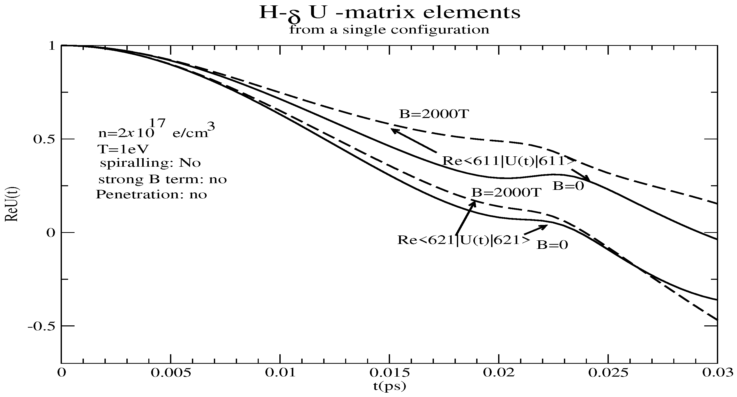
where is the Schrödinger representation of the emitter–plasma interaction and is the energy of the ith state of the atomic Hamiltonian plus the magnetic field. For hydrogen lines without a fine structure and the linear Zeeman effect, and assuming that the emitter–plasma interaction is dipole, the difference in the magnetic quantum numbers of and is and can take the values 0 (if , and , with the Bohr magnetron. Zero is the result we receive from the interaction component parallel to the magnetic field (the “adiabatic” component) and from the perpendicular (“nonadiabatic”) component. In frequency units, the nonadiabatic energy difference is about , with B in Tesla. For those collisions with duration such that , oscillations are fast and in fact inhibit memory loss, as and change signs too rapidly on the inverse HWHM time scale (which is typically for electrons ). As a result, this translates into a slower memory loss, and hence smaller widths. Refs. [3,4,5] employ the perturbation theory, but the idea is valid in general [10,11,12]. In Figure 1, we show diagonal matrix elements for the line for a single (the same) realization of the plasma electron and ion microfield (called “configuration”) with and without a magnetic field. In this calculation, the magnetic field is taken to have no other effect except for Zeeman splitting.
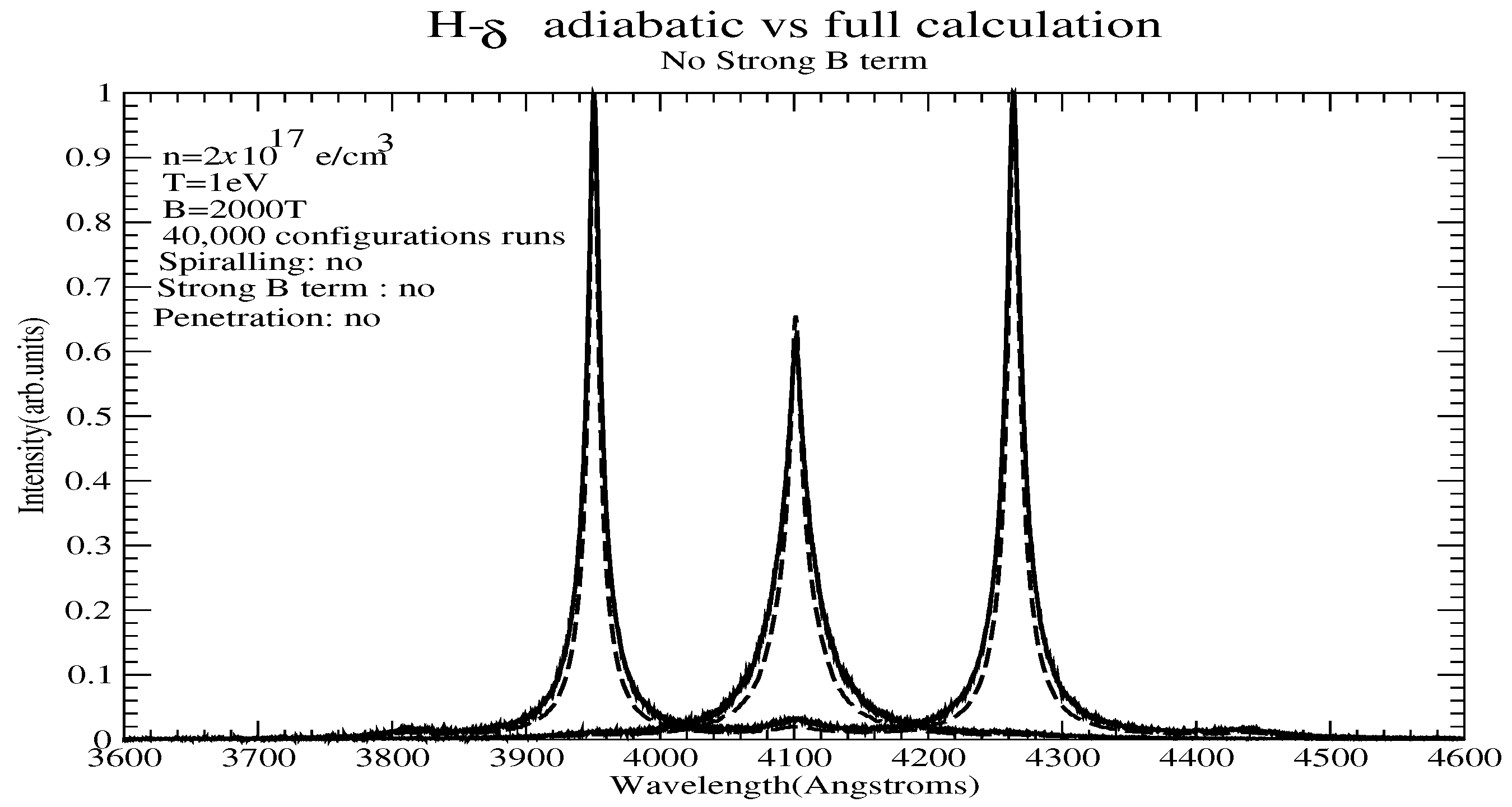
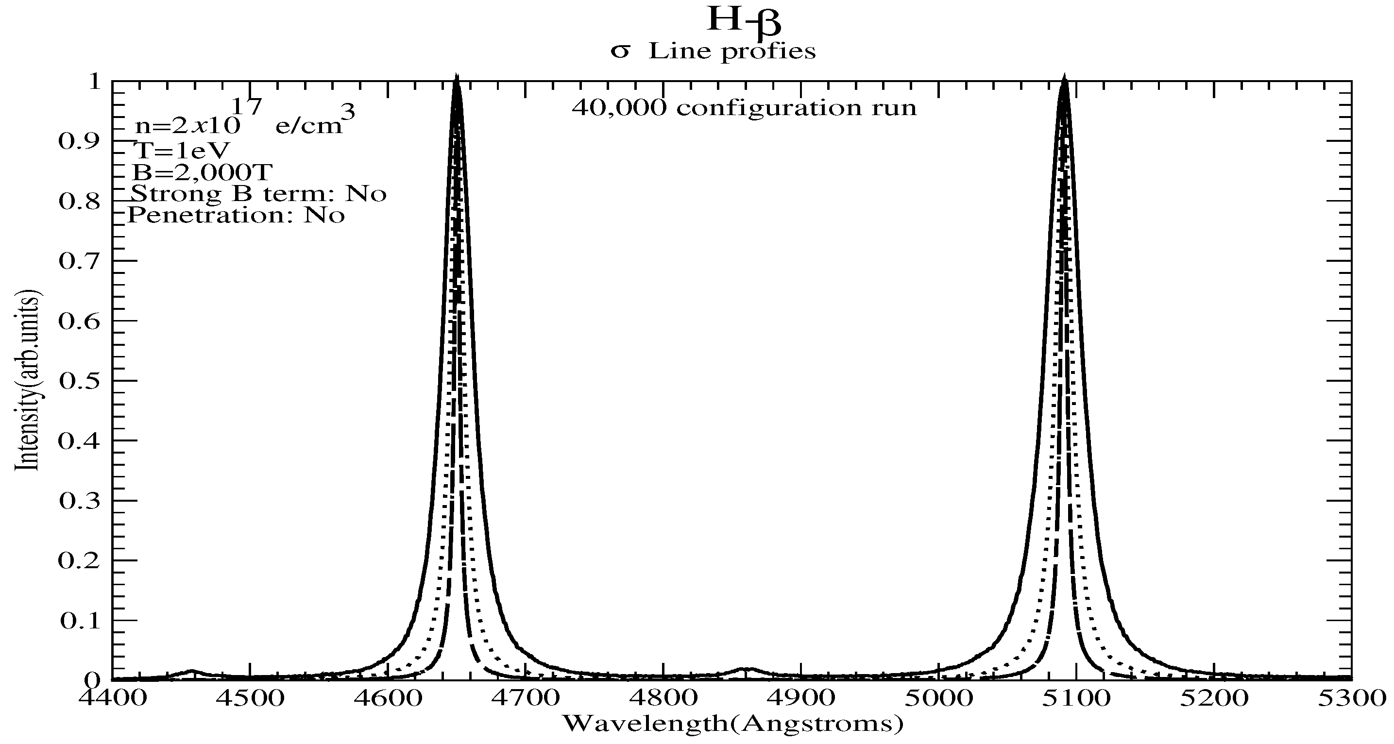
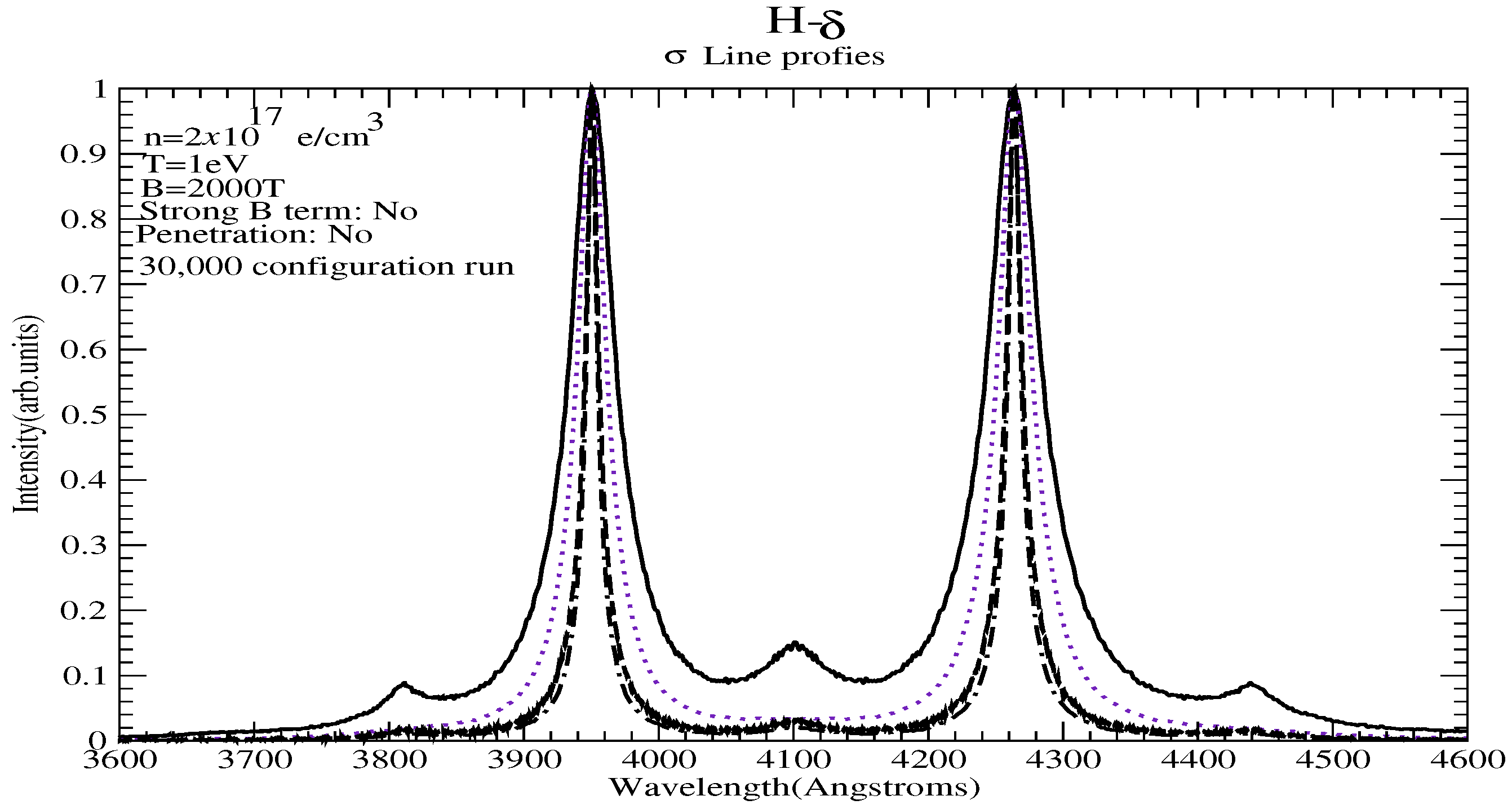
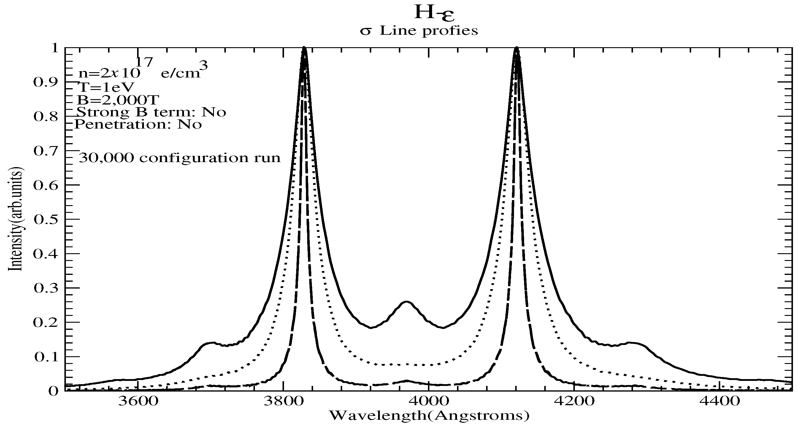
However, this is a linear Zeeman effect prediction and it is not clear that for large magnetic fields [13,14], the nonadiabatic term is always negligible. To check the relative importance of adiabatic vs. diabatic contributions, calculations were repeated by artificially setting for all matrix elements between all upper level states’ combinations ( − ), and similarly for the lower level states . Figure 2 shows the results, without spiralling for the line, without the strong B term accounted for. We use the term “strong B term“ to mean the term quadratic in B as in [13,14]. Indeed, as expected from the argument above, the adiabatic contribution dominates, although the difference is larger than the 1% figure quoted (for instance, in [5] for ).
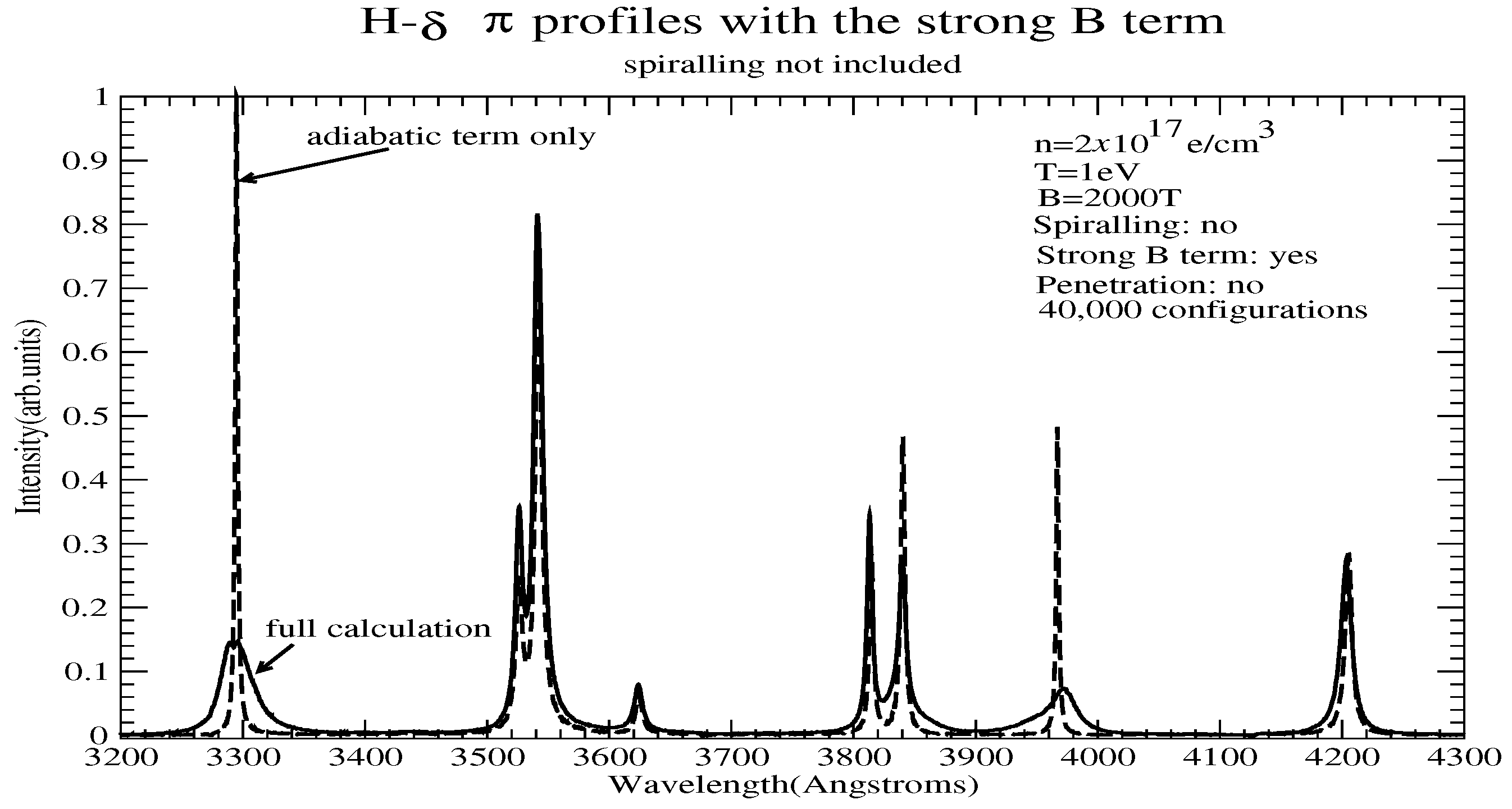
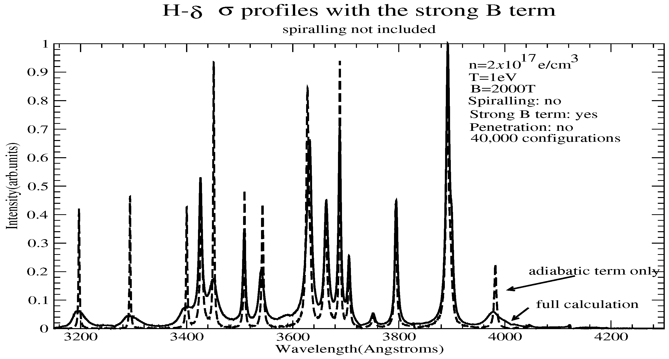
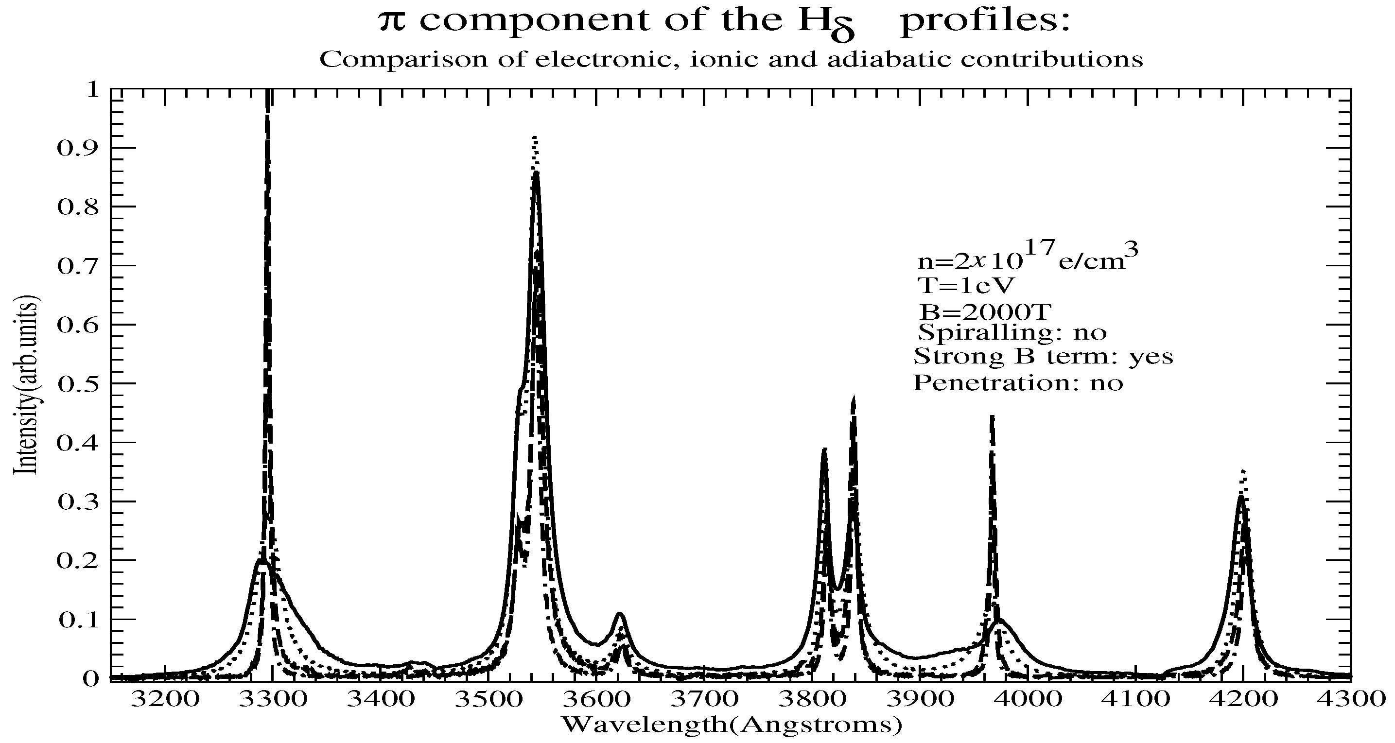
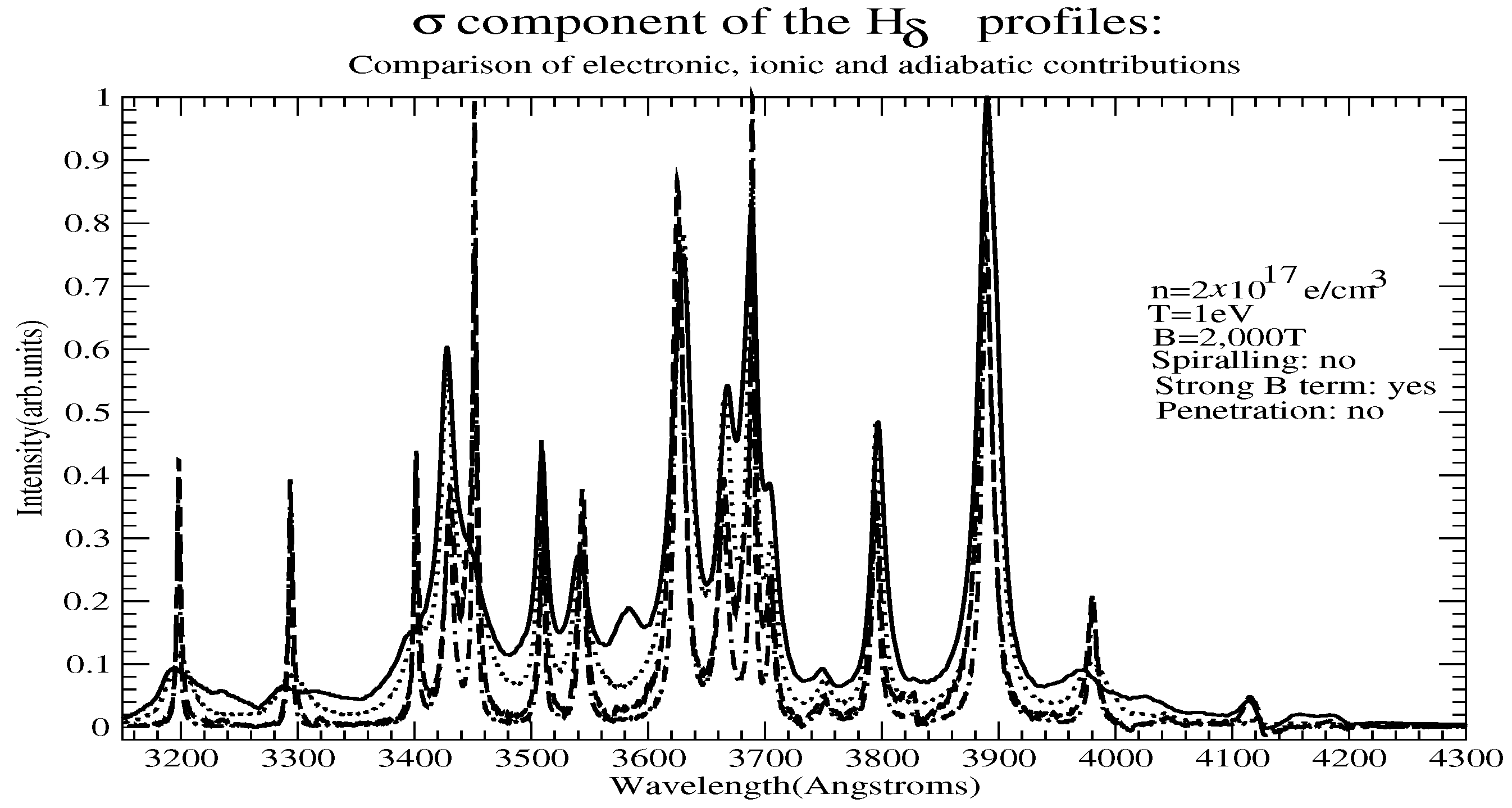
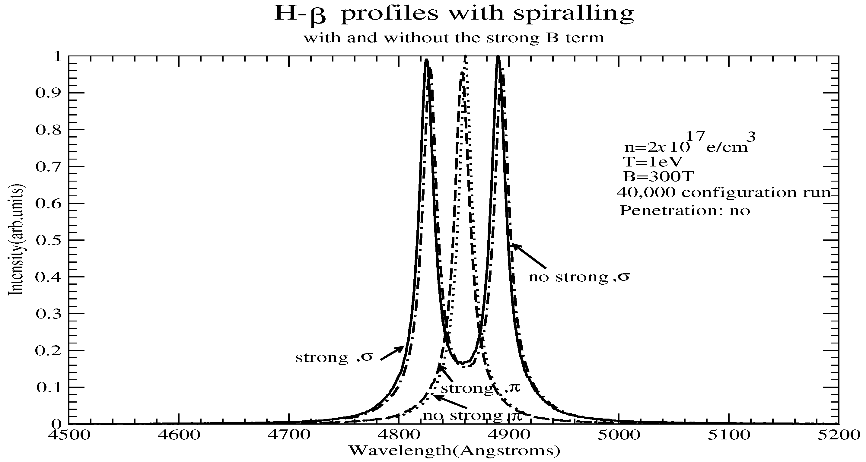
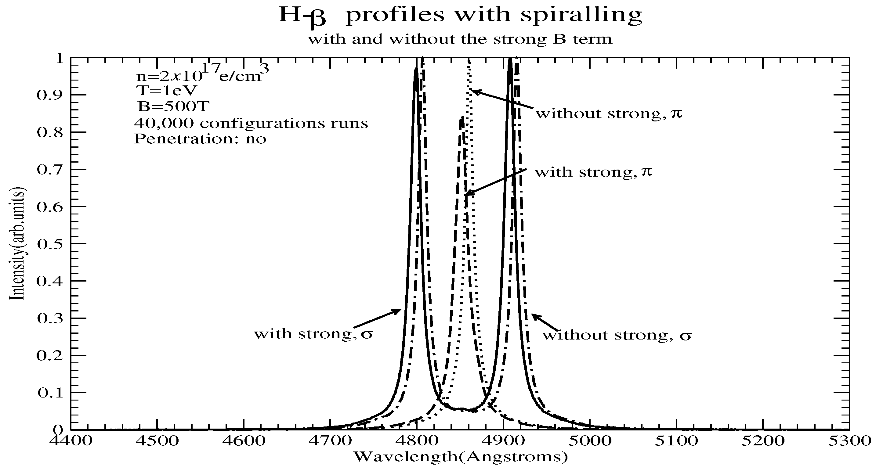
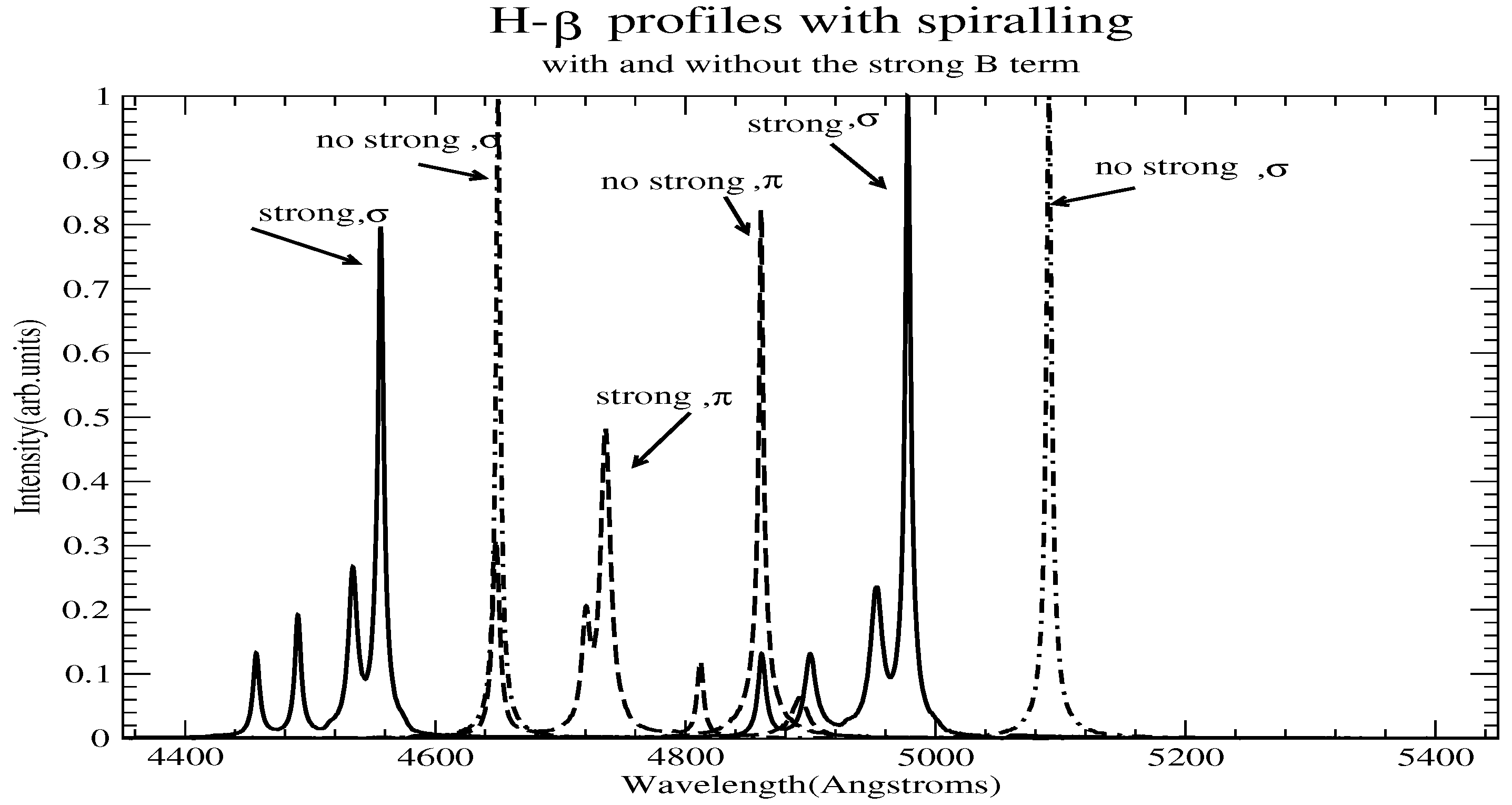
Figure 3 (for the component) and Figure 4 (for the component) show the results once again without spiralling for the line, but this time, with the strong B term accounted for. For some peaks, the full and adiabatic calculations are indeed close, but for others, there is a substantial nonadiabatic contribution. The point is that for conditions of interest to white dwarfs, the magnetic perturbation is not necessarily small, and this results in a complete renormalization of the energy structure and profile.
Ions are neglected in [3,4,5], and this is qualitatively correct, as discussed below. A very important point is that with spiralling trajectories, the collision volume, and hence contributing plasma particles, are different [15,16]. Although spiralling trajectories roughly cover more phase space, this is offset by the fact that this contribution is partial, and using an unscreened interaction for particles beyond the screening length can severely overestimate the widths.
2. Remarks on the Calculations
To keep the calculations comparable to the suggestions mentioned, all calculations: (a) assume hydrogen lines without fine structure; (b) only consider states with the same quantum number in the time evolution of the upper and lower states, respectively; and (c) only take into account dipole interactions; thus, penetrating collisions are not taken into account, i.e., the long-range dipole approximation is used for the interaction even when the colliding plasma electron is inside the wavefunction extent of the emitter. However, (Debye) screening is accounted for all collisions, as this is important. Hence, calculations are performed with and without the account of spiralling and, in some cases, are labelled “With Strong B term” by considering not just the linear term, but the full Hamiltonian with the magnetic (B) field, i.e., including the term quadratic in B [13,14]. This results in a renormalization of the spectrum and the appearance of new components, as already shown in Figure 3 and Figure 4. The code identifies the renormalized peak positions and computes an autocorrelation function for each such line. We also do not consider the effect of the magnetic field on the plasma distribution functions.
When spiralling is taken into account, this is performed by taking full account of all relevant perturbers (plasma electrons and ions–protons in our case, unless specified otherwise), using the collision time statistics method [15,16]. Specifically, to take account of all perturbers that become relevant during a time T (the point of the collision time statistics), which is a few inverse widths of the line in question, we consider a “collision volume”, which is the number of particles divided by the density. Ions are treated on an equal footing as electrons, so both static and dynamic ion effects are accounted for. This is in principle important, because increasing the memory loss time (e.g., decreasing the broadening) provides ions with more time for their motion to become appreciable, although for weak magnetic fields, this makes little difference widthwise for lines without a central component, such as and . For straight line trajectories, this volume is a cylinder with radius and length with , the range in times of closest approach , which is a function of v and :
where and is the shielding (Debye) length, so that perturbers that do not come closer than at any time in (0, T) can be neglected. For spiralling trajectories, the volume is:
with
and
with the one- and two-dimensional Maxwellian distributions
and
respectively, for the parallel and perpendicular to the magnetic field velocity components and the Larmor frequency, :
where B is the magnetic field, Q is the perturber charge, and m is the perturber mass. This is efficient for electron perturbers and, as discussed in [15], typically results in a smaller number of contributing electrons, since only the parallel velocity () component is relevant for the cylinder length. In the calculations, the extension of this method that also makes it efficient for low-velocity perturbers (or small B) [16] was used. In the comparisons, we also use the dimensionless value
which is essentially the ratio of the screening length to the average Larmor radius . Note that is proportional to , whereas the corresponding quantity for nonspiralling trajectories was proportional to . To the extent that this term dominates, it means that less electrons are effective because the average of a 3D Maxwellian is larger than the average of a 1D Maxwellian. Hence, we expect a line narrowing in that case. However, as the tables show, is either about equal, larger, or even dominates (for ) for ion perturbers.
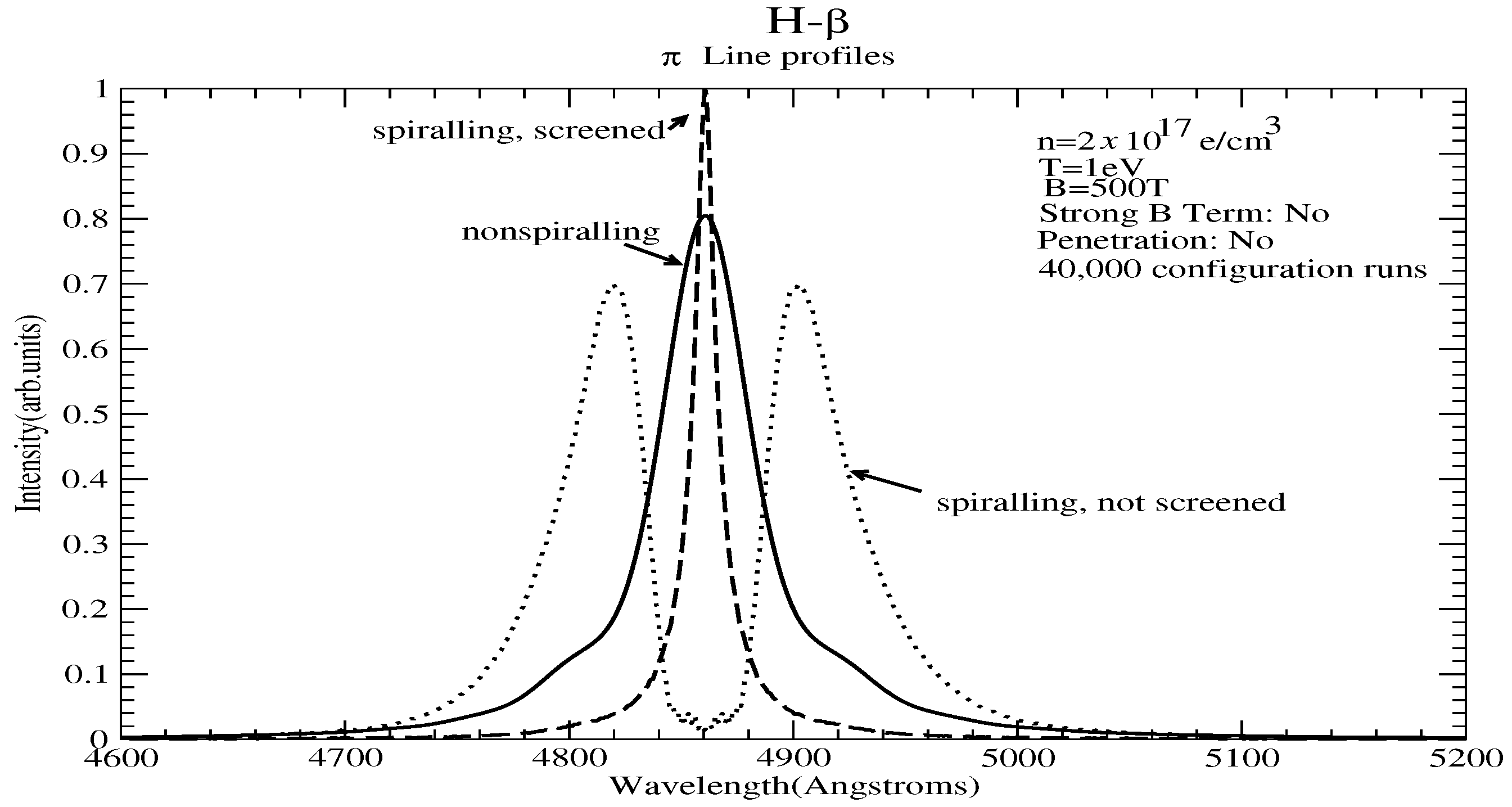
All calculations are carried out at an electron density of 2 × 10 e/cm and a temperature of 1 eV. Three different magnetic field strengths are considered, namely 300, 500, and 2000 T, which are relevant for white dwarf conditions and were chosen so that the claimed validity condition [3,4,5] is fulfilled, as well as to showcase the importance of the quadratic B-term. (Debye) screening is explicitly included in all calculations shown here over the entire electron or ion path. It is important to note that the ratio of the average Larmor radius to (which the collision time statistics method takes equal to 3 times the screening length) for electrons ranges from 0.225 to 0.03 for the magnetic fields considered. This means that using an unscreened interaction as in [3,4,5] can seriously overestimate the contribution of electrons close to the screening length and the widths. For example, in [5], Equation (1) uses an unshielded interaction with Equation (23), limiting impact parameters inside the Debye length. However, the unshielded interaction is reasonable for perturber (i.e., electron) distances smaller than the shielding (Debye) length. These distances are not the impact parameter (even at the time of closest approach), unless the Larmor radius is much shorter than the impact parameter. As shown in Table 1, Table 2 and Table 3, the Larmor radius for the fields considered ranges from 10 to 67% of the Debye length (notice that is 3 times the Debye length in this work). Hence, the use of an unscreened interaction even at distances of 1.67 times the shielding length understandably overestimates the strength of the interaction and consequently the broadening. We illustrate, by plotting in Figure 5 for the line, profiles at B = 500 T without the strong B term from the present approach, using: (a) a shielded interaction for both electrons and ions, as is used throughout this work (dashed); (b) an unshielded interaction for both electrons and ions (dotted); and (c) the corresponding calculation without spiralling (solid). It is seen that using an unshielded interaction results in a substantial increase over the nonspiralling result. As discussed above, broadening is dominated by electrons in both the shielded and unshielded cases.
3. Role of Ions
The quoted references [3,4,5] and, indeed, most works, neglect ions or treat them within a quasistatic approach. In the present approach, ions are treated on an equal footing as electrons, using the collision time statistics approach [16], which guarantees that every particle that is relevant (i.e., contributes non-negligibly by entering the shielding sphere anytime in (0, T), with T a few inverse HWHMs, so that the autocorrelation function is non-negligible), is accounted for. Although ions contribute significantly, or even provide the most important contribution for the case without a magnetic field (as shown, for example, in Figure 6), electron broadening dominates for the magnetic fields considered here, whether spiralling is accounted for or not. Hence, we first discuss how ions are affected by the magnetic fields studied, and second, how spiralling affects them.
3.1. Ions without Spiralling
As discussed, the Schrödinger equation determining the evolution of the atomic states, reads
where U is the time evolution operators, , with as the dipole operator and (t) as the random particle field, and
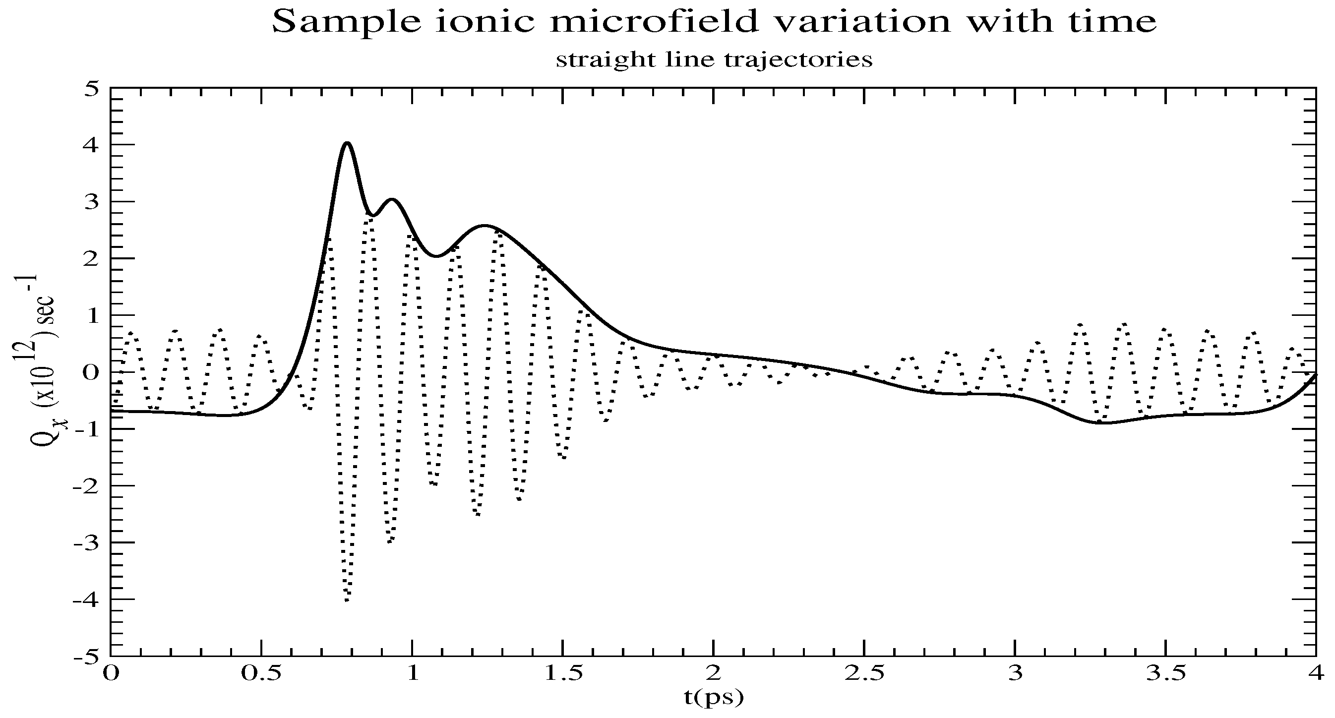
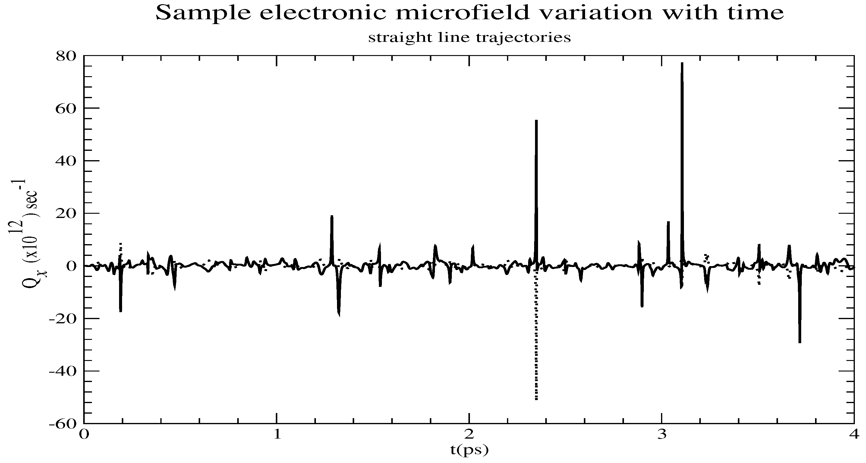
To illustrate, we plot in Figure 7 the quantity , where is a random ionic field in the x direction, computed without the account of spiralling, shown as a solid line. This, except for a numerical factor corresponding to the dipole matrix element in atomic units, is the x-contribution to .
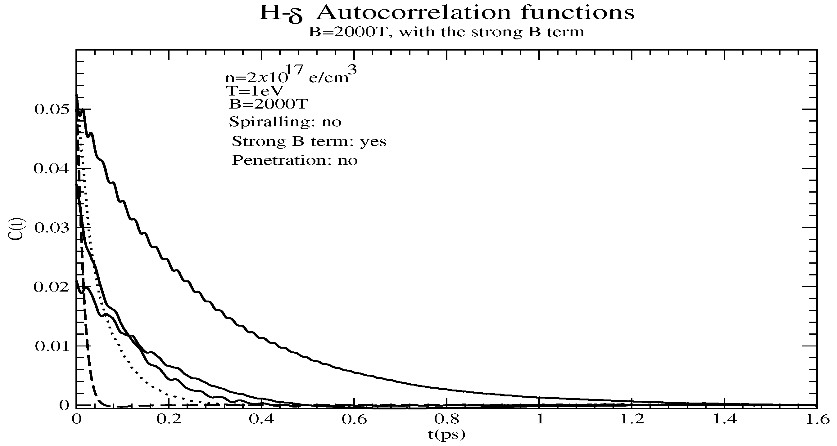
To show in a simple way the effect of the Zeeman splitting, we also multiplied, in the same figure, by cos(, with as the Zeeman splitting (dashed line). It is clear that oscillates fast, and hence, the sign of changes. This leads to a significant delay in the decay of the autocorrelation function, and hence, smaller widths [10,11,12]. This is shown in Figure 8, which shows the real part of the autocorrelation functions (the Fourier transforms of the line profiles) of four different components of the line under a magnetic field of 2000 T, taking into account the strong B effects, but not spiralling. Compared to the B = 0 (dashed line) autocorrelation function, the decay of is significantly slower (hence resulting in smaller widths) and three of these components (solid line) display a sawtooth shape, demonstrating the effect just discussed, i.e., the changing sign of .
In contrast, for electrons (Figure 9), because the field consists of sharp “spikes”, does not oscillate as rapidly on the spike time scale, and hence, the decay of the electron-perturbed autocorrelation function is not delayed as much, i.e., the widths are not affected as much as for ions.
As previously discussed, when strong B effects are important, and as, for some components, the energy separation can be smaller than the Larmor frequency, the nonadiabatic effects are important and ions are in general not to be neglected. This is illustrated for the line at B = 2000 T, where we separately show, for the (Figure 10) and (Figure 11) components, the profile with nonspiralling electrons and ions (solid), the adiabatic component of nonspiralling electrons and ions only (dashed), nonspiralling electrons only (dotted), and the adiabatic component of nonspiralling electrons only (dash-dotted). Although the adiabatic ion contribution is often fairly minor, it is clear that for some components, the nonadiabatic contribution and the ionic contribution are substantial.
3.2. Role of Spiralling
As shown in Table 1, Table 2 and Table 3 for electrons, the parameters considered are the typical gyroradius , with as the velocity component perpendicular to the magnetic field and as the electron Larmor frequency. For ions, however, , as shown in Figure 12, except for the highest field considered, where they are comparable. Specifically, relevant impact parameters for are in , which is the smallest ) for (even if is slightly smaller than ). Another important difference is that the time of interest (of the order of the inverse HWHM) corresponds (in the case of ) from 50 to 350 electron Larmor periods, while for ions: from roughly 1/20th to a third of a Larmor period. The and shown in these tables are for both electrons (subscript e) and ions (subscript i). For electrons , the term proportional to dominates, while for ions, the term is at least comparable to . The number of contributing electrons decreases with B, while the number of ions increases. This trend for ions will eventually be reversed for a large enough B, where the Larmor radius becomes smaller than the shielding length. Nevertheless, for the parameter range considered, the ionic contribution is very small, as only impact parameters in () contribute, and these contribute only over a part of their trajectory and practically when they are in the plane through the emitter that is perpendicular to the magnetic field. The result is that Zeeman splitting reduces the ionic contribution much more than the electronic one and spiralling brings about a further significant reduction in the ionic contribution.
4. H- Line
In this and the following two sections, calculations for three Hydrogen lines mentioned in refs. [3,4,5] are presented. The structure of these calculations is as follows. First, a comparison of the spiralling and nonspiralling trajectory results is shown for all three magnetic fields (300, 500, and 2000 T), neglecting the quadratic term in the magnetic field. This shows the effect of spiralling alone. Next, again neglecting the quadratic term in the magnetic field, calculations are shown with and without spiralling, where: (a) only the plasma electrons are considered and (b) both the plasma electrons and ions are accounted for the computation of the broadened line profile. The point is, of course, to assess the relative importance of electron vs. ion broadening. Lastly, the calculation is repeated with the quadratic term in the magnetic field and the profiles with and without that term are compared (both with spiralling accounted for). In this way, the effects of spiralling and the quadratic term are investigated separately.
4.1. Profiles without the Strong B-Term
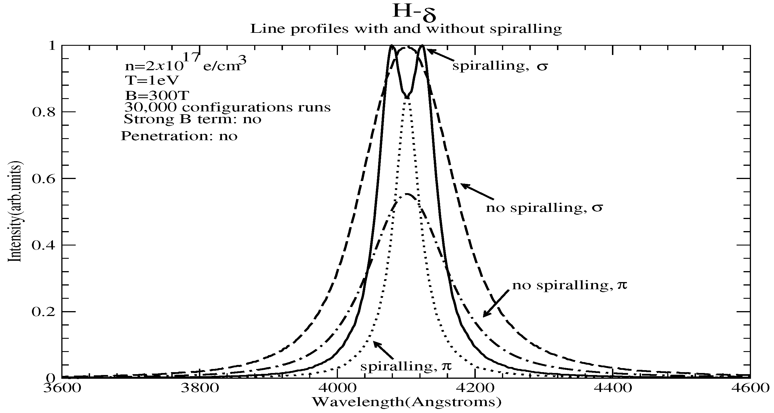
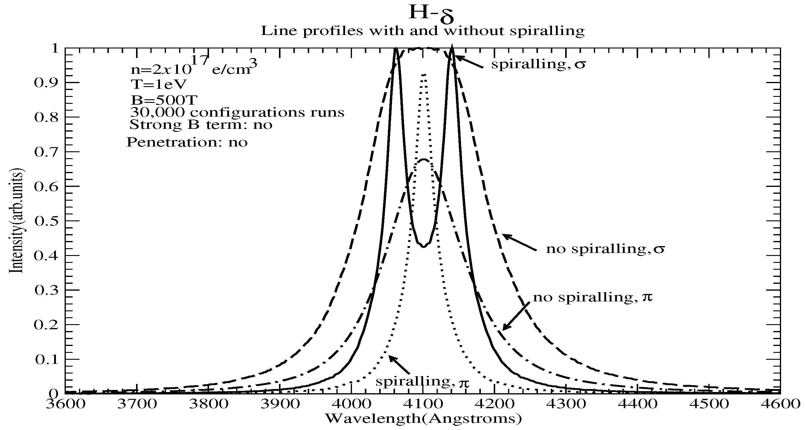
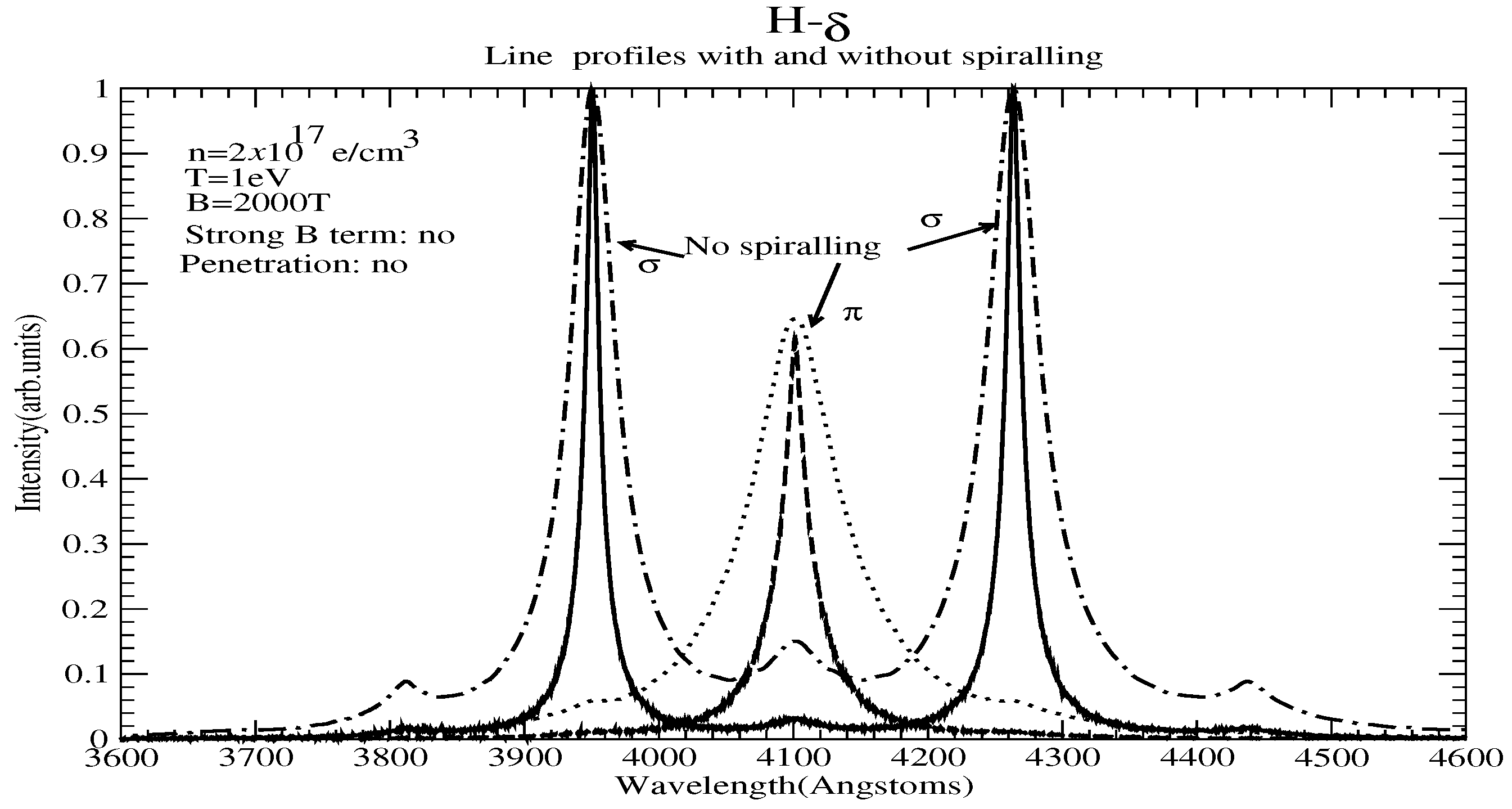
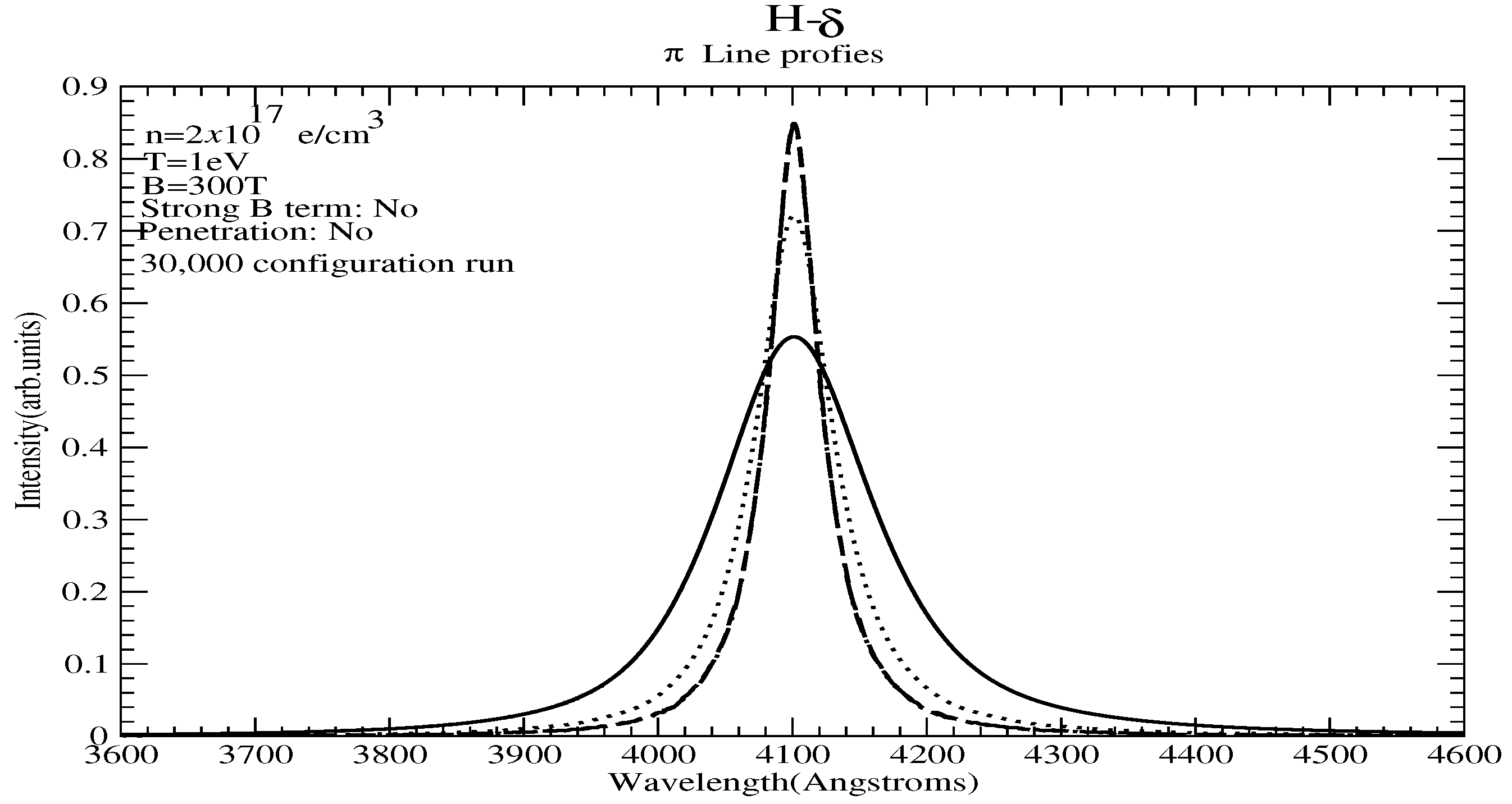
In this section, we compute line profiles for the H- line with and without spiralling. Neither penetration nor strong field effects (e.g., the term in the Hamiltonian) are taken into account. First, the profiles with and without spiralling are shown for an electron density of , temperature eV, and magnetic fields of (a) 300, (b) 500, and (c) 2000 T, with only the linear B-field term. All these fields are larger than the limit, above which spiralling is considered to result in a significant width increase, according to [3,4,5].
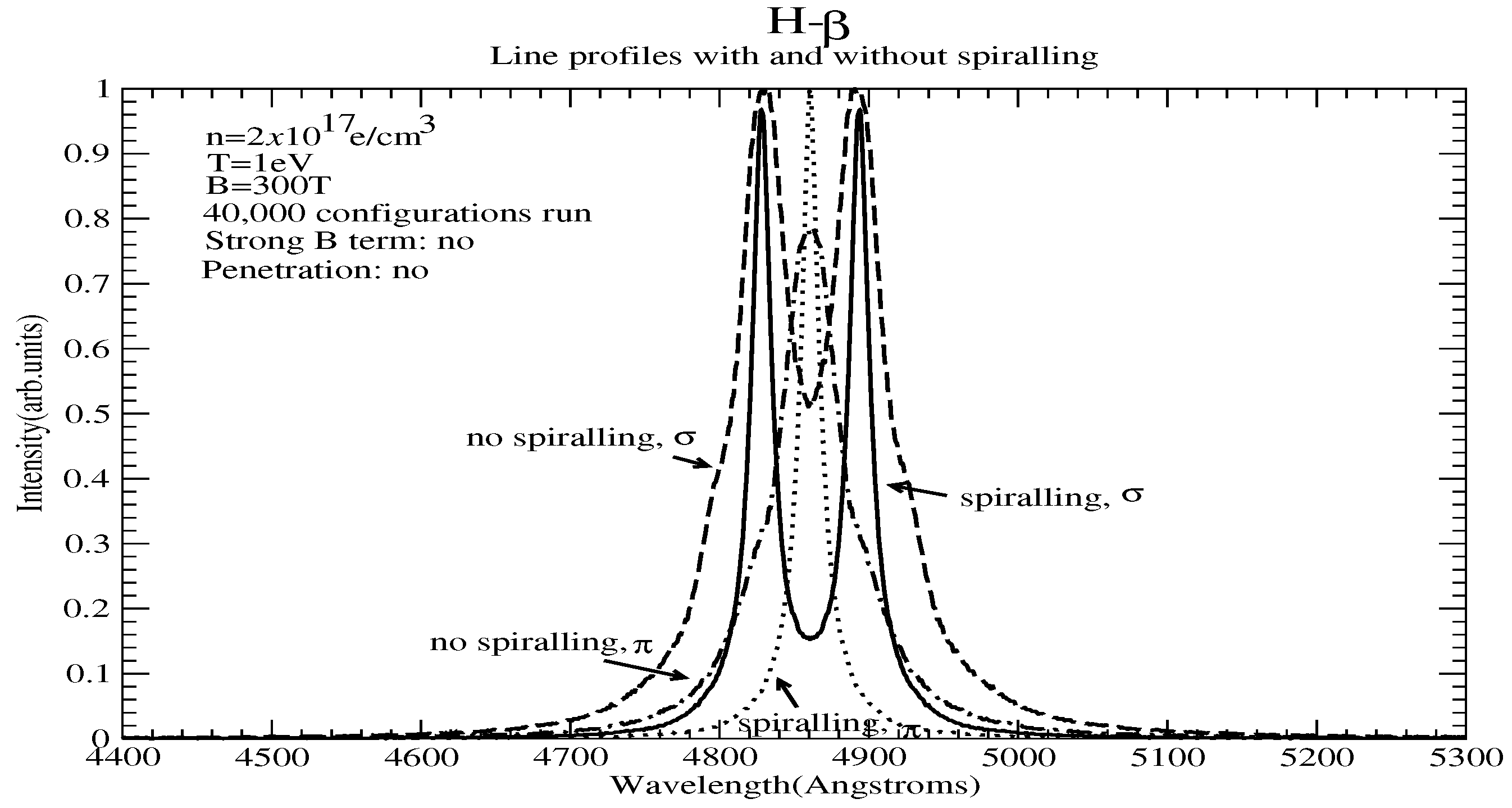
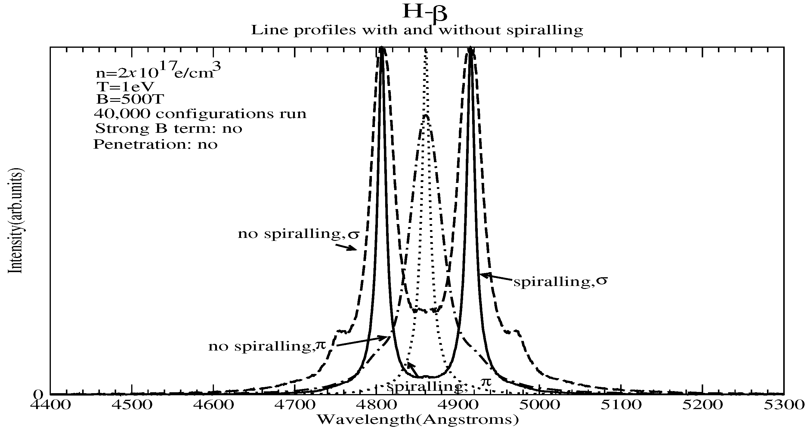
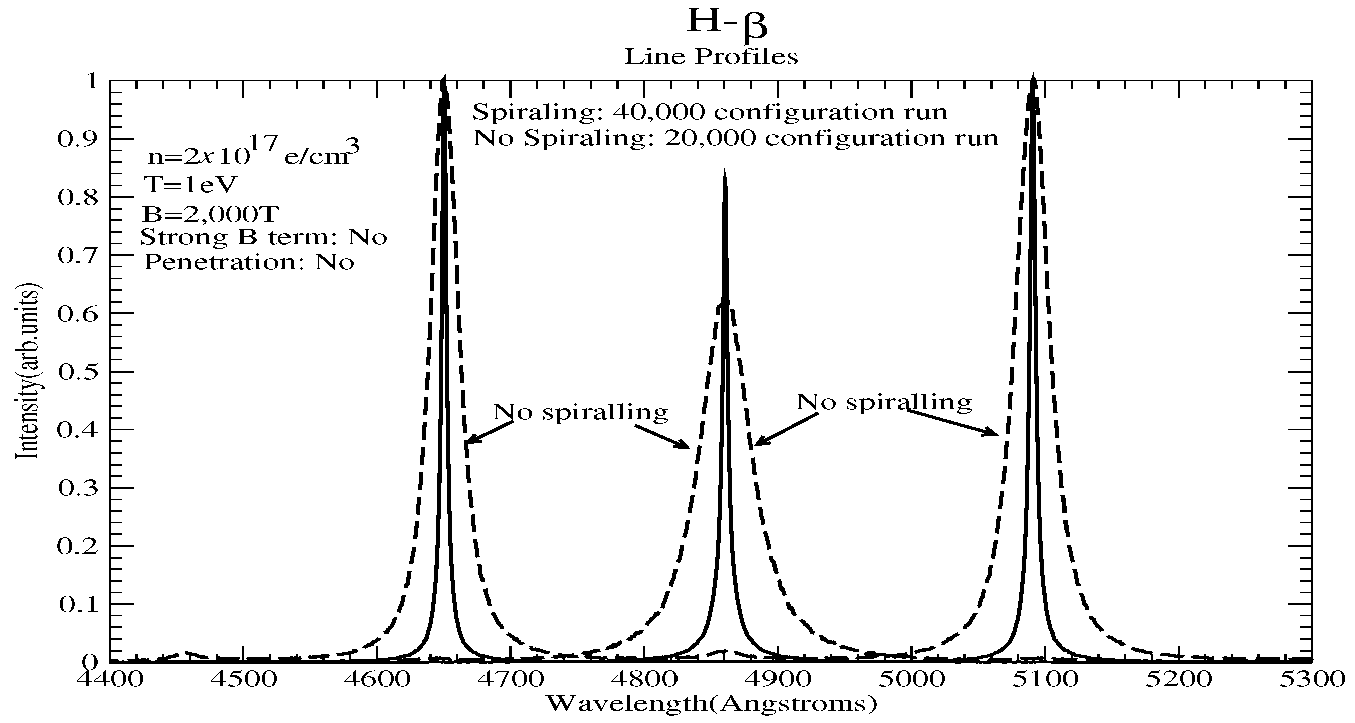
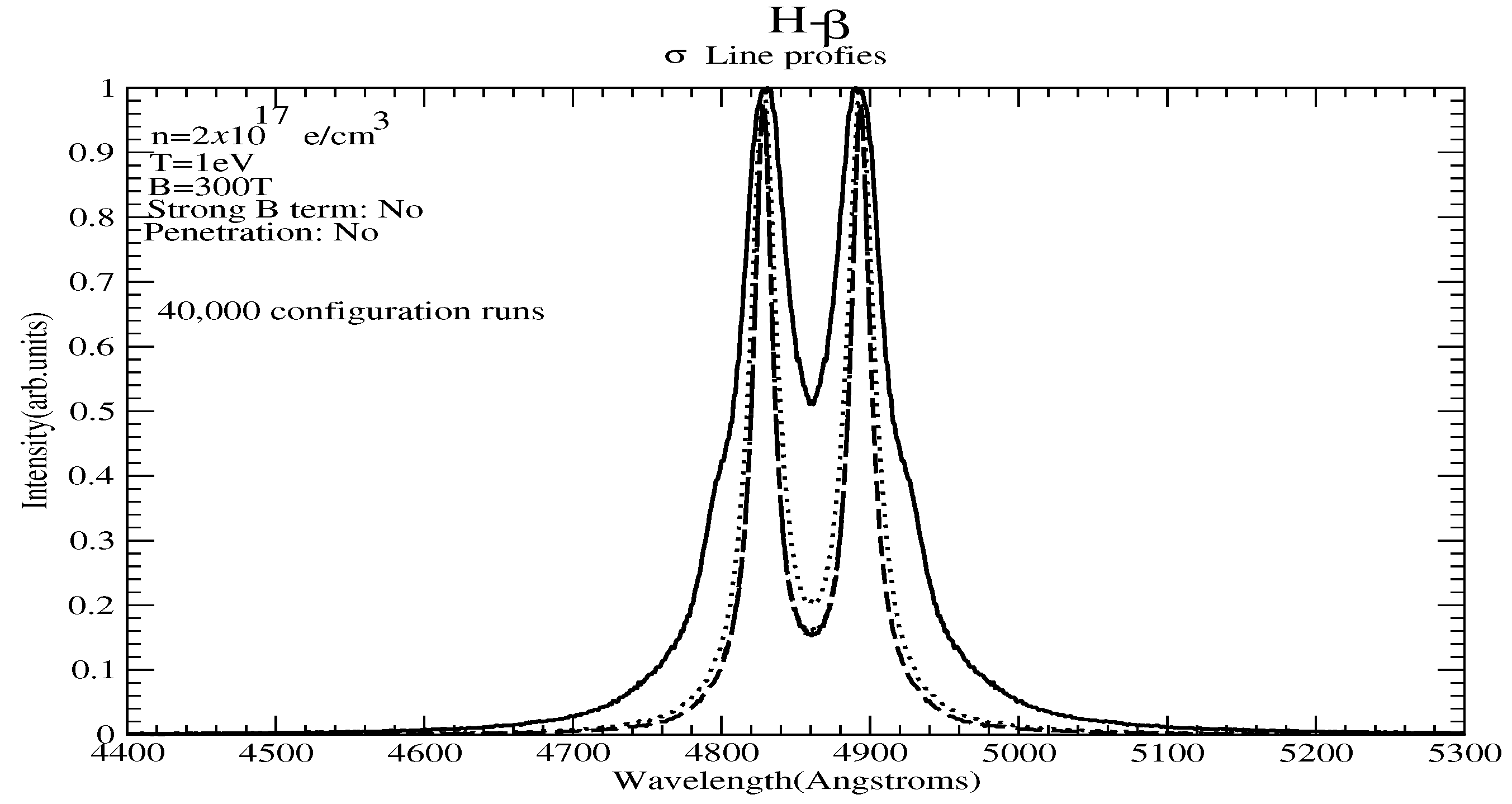
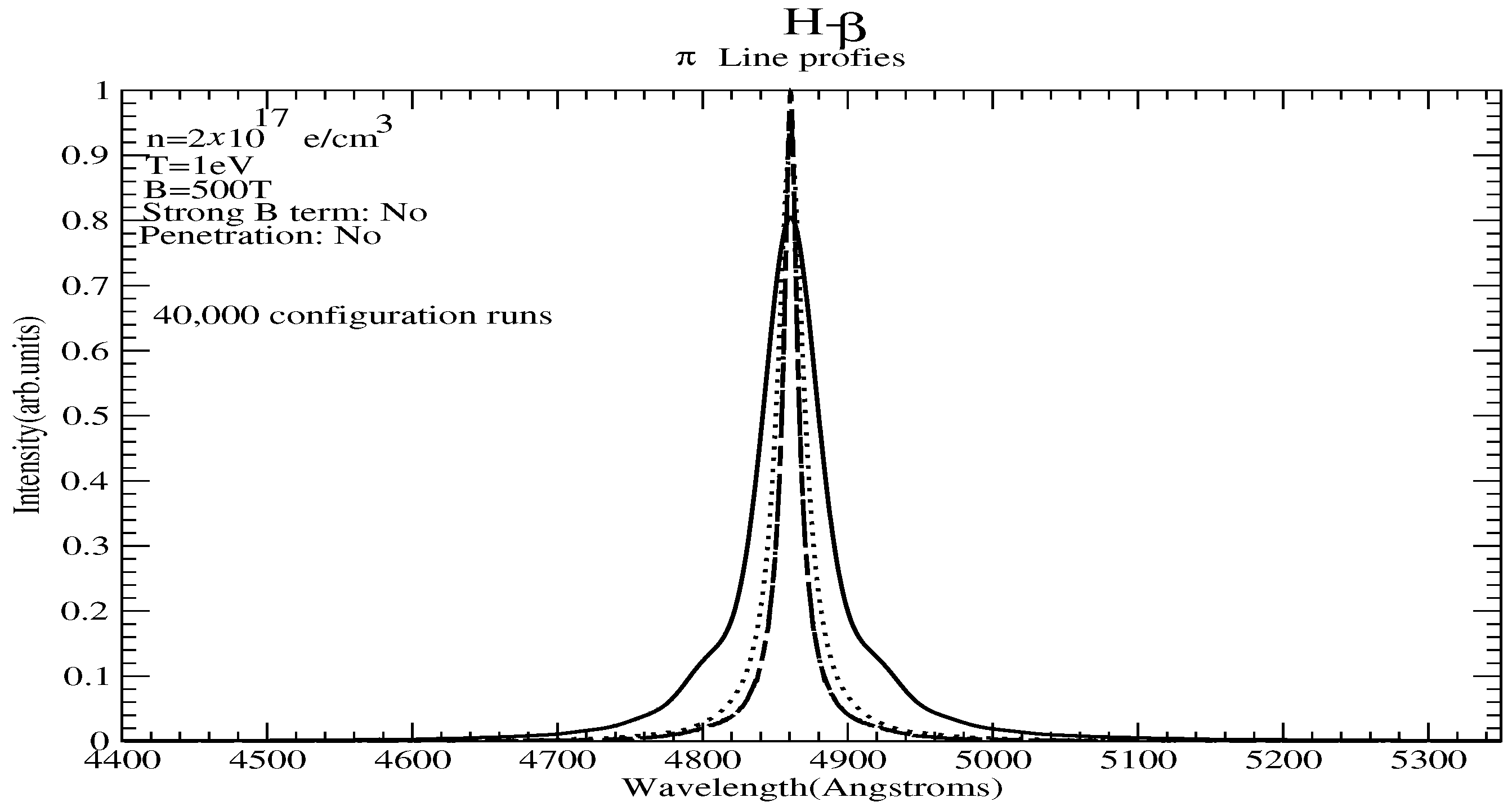
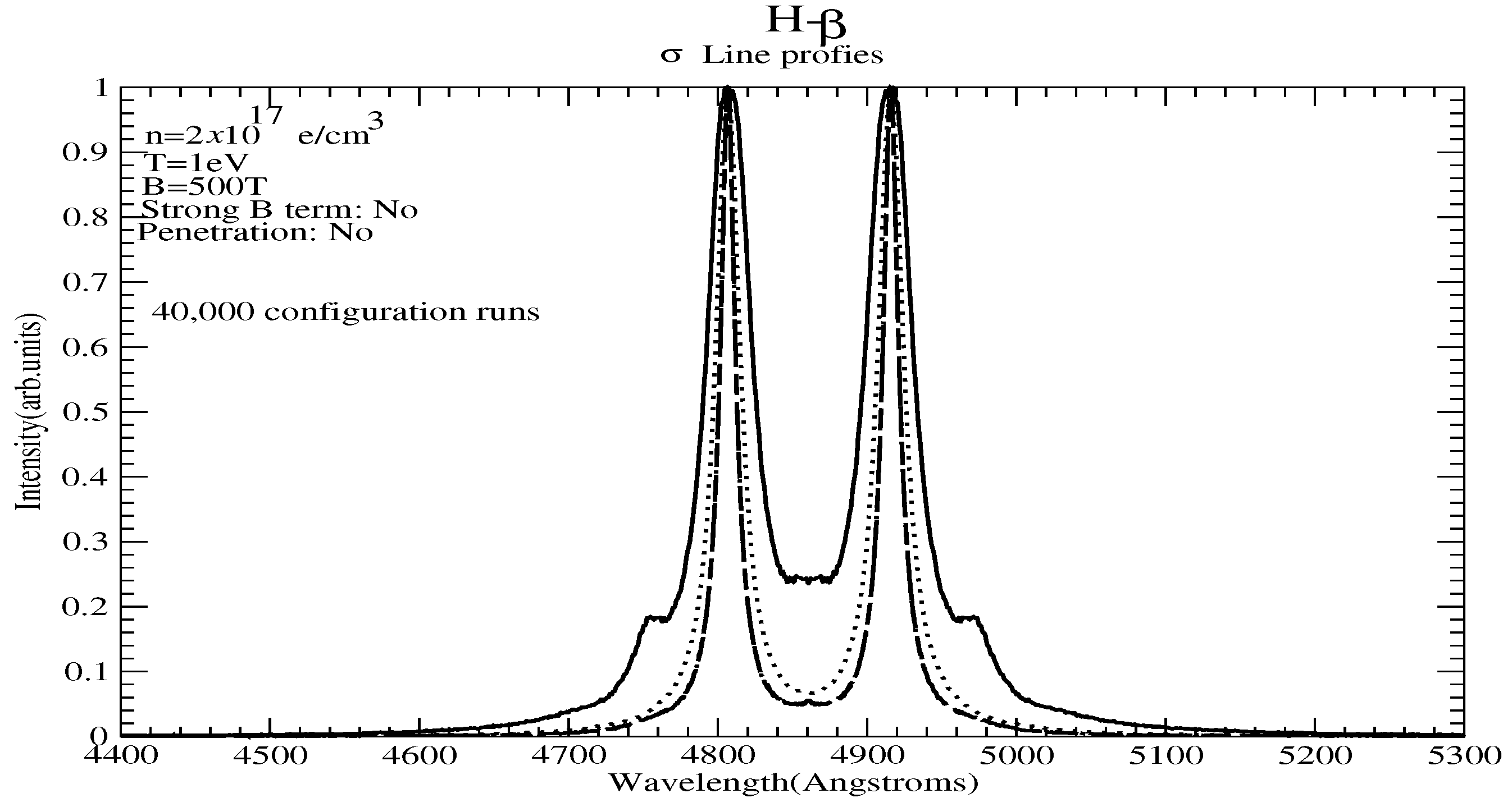
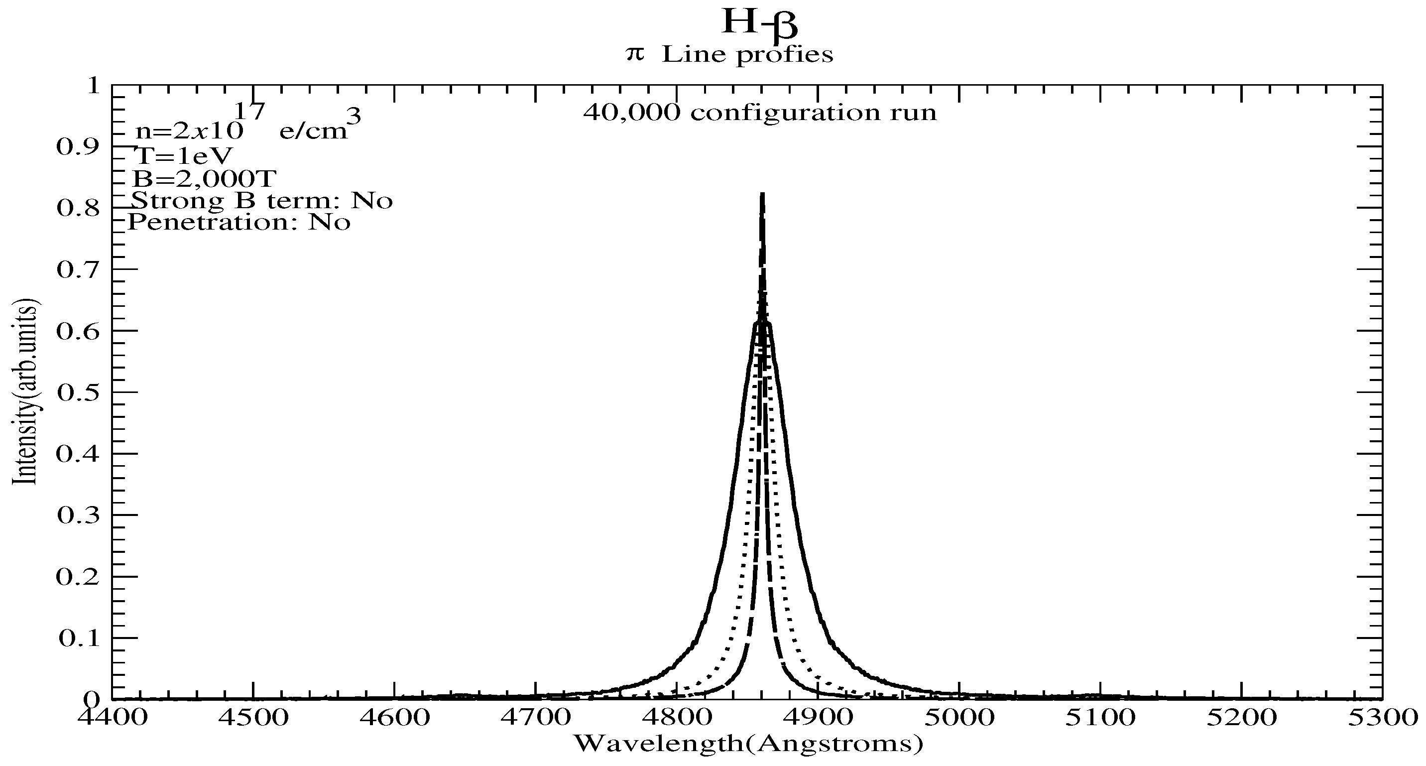
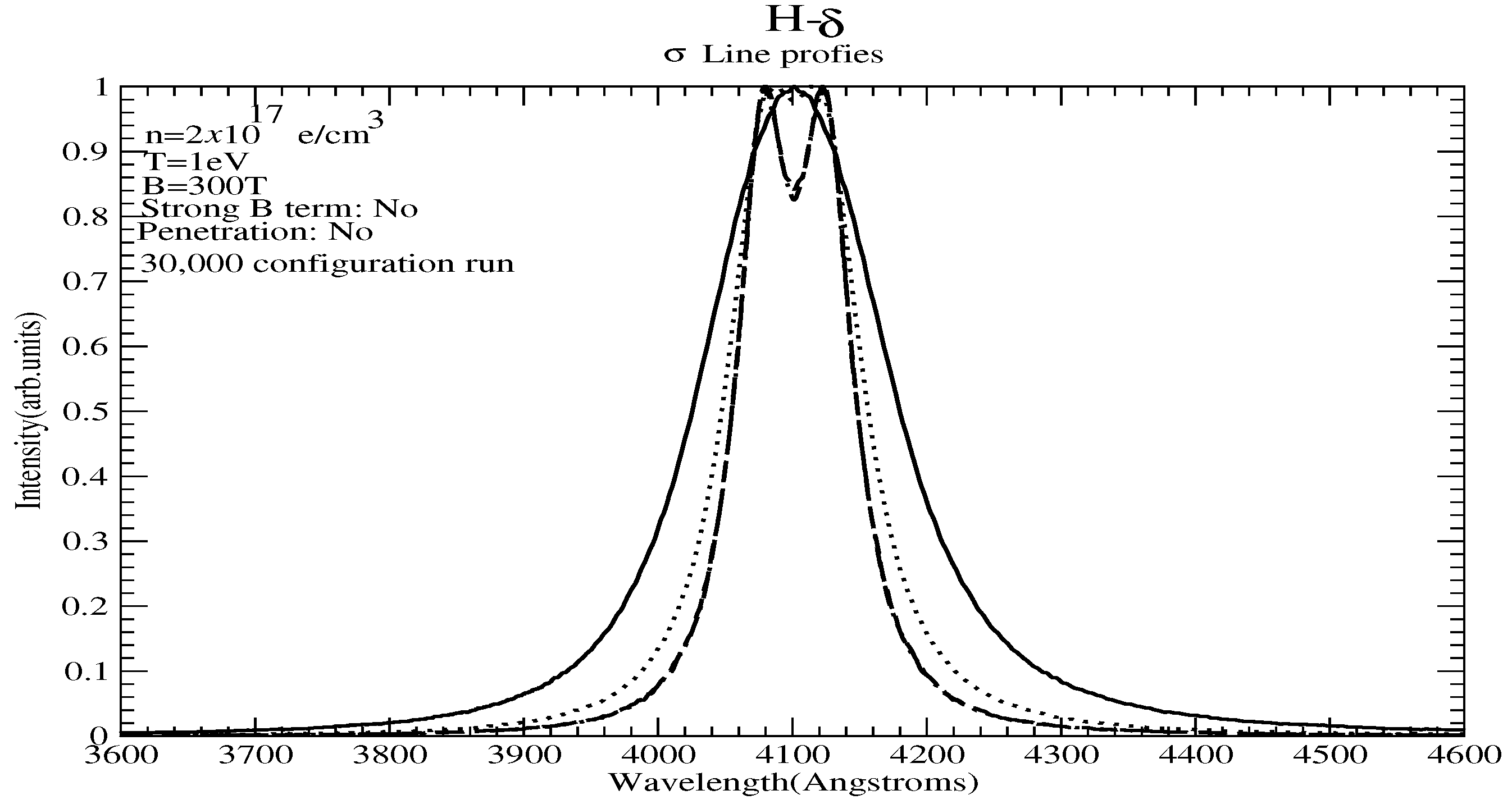
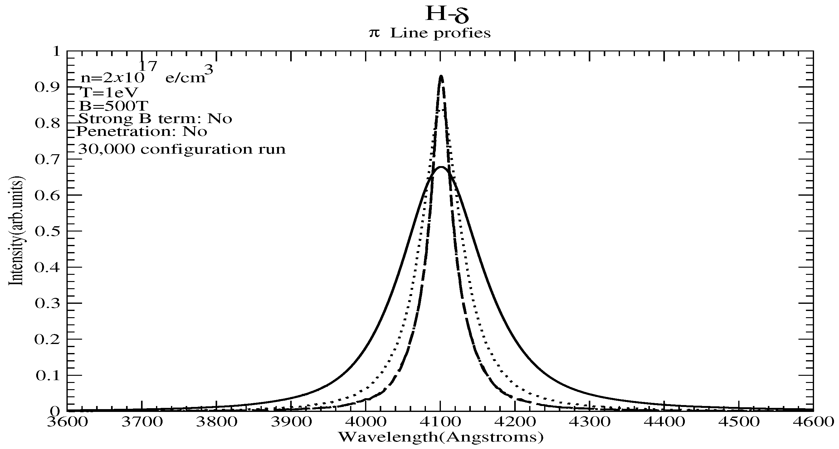
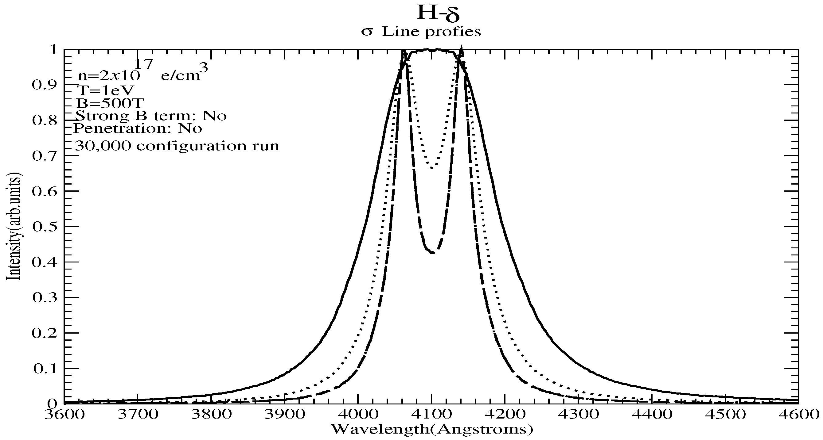
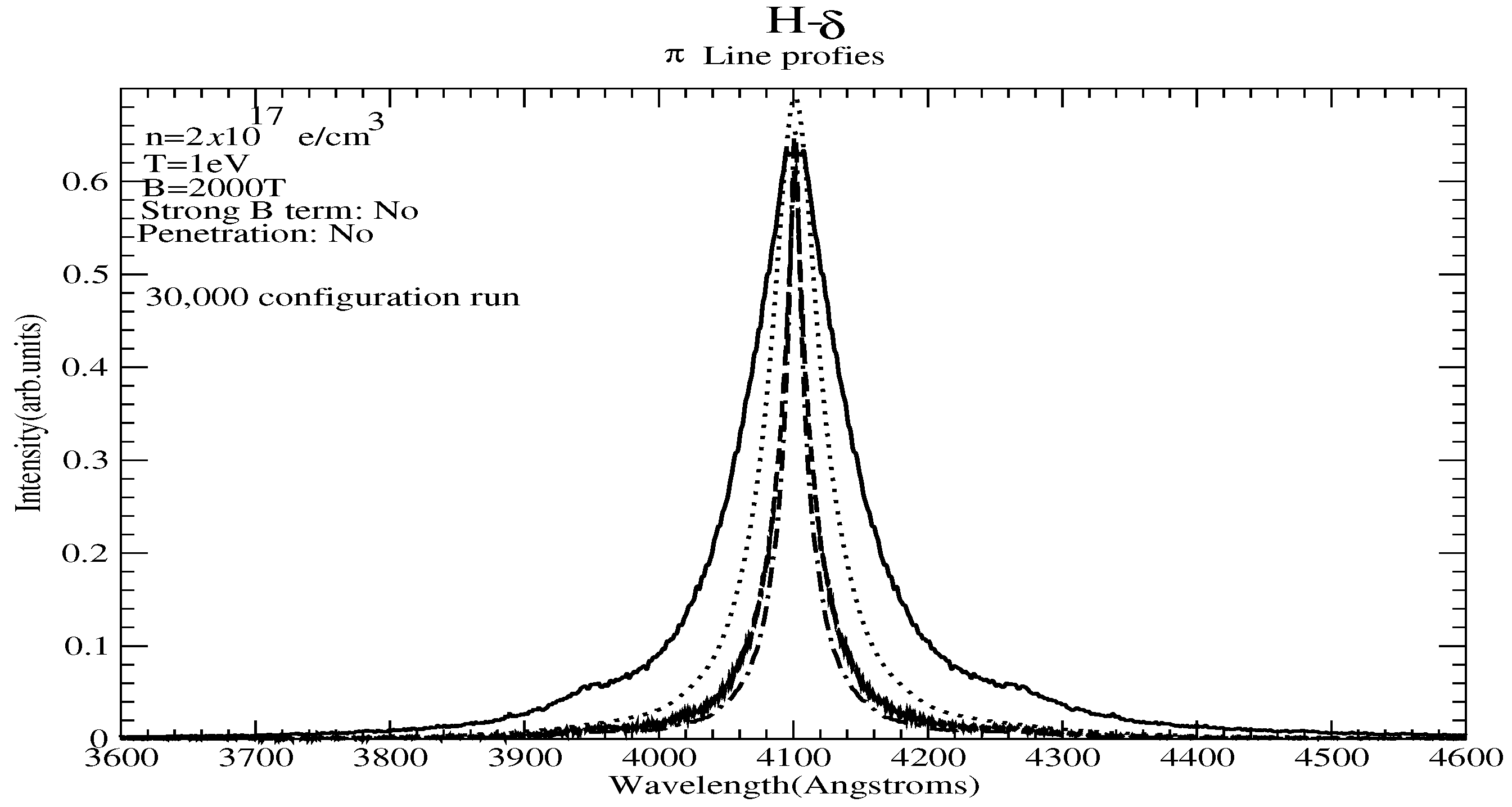
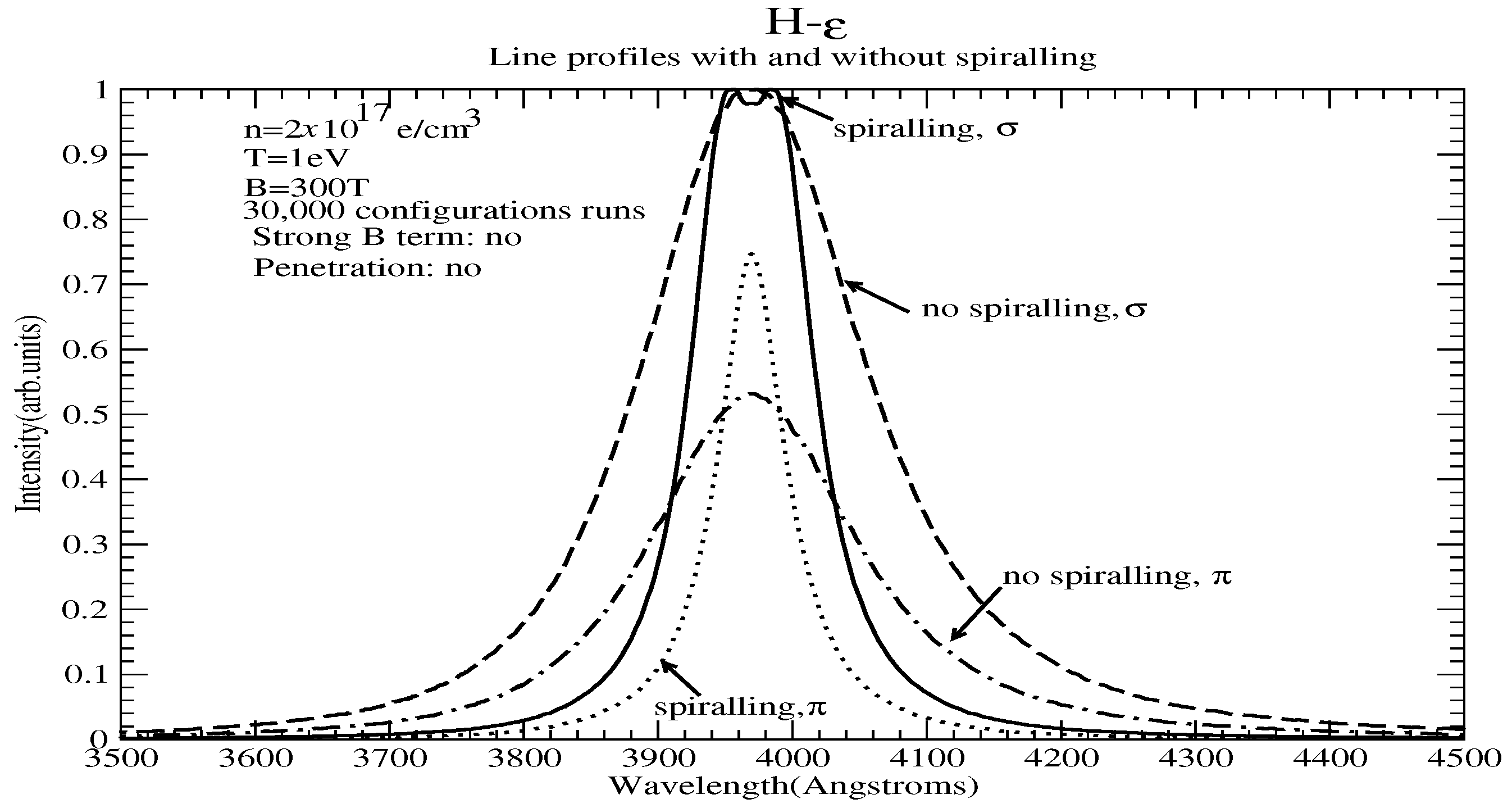
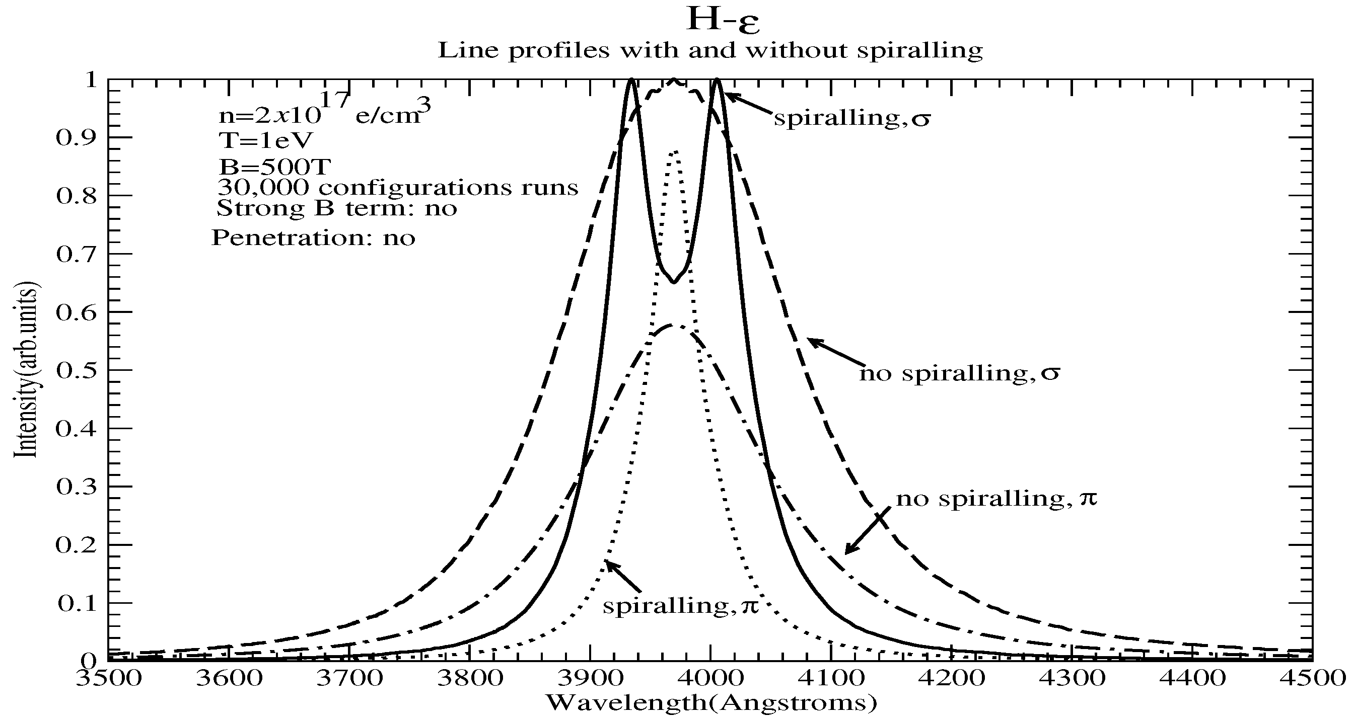
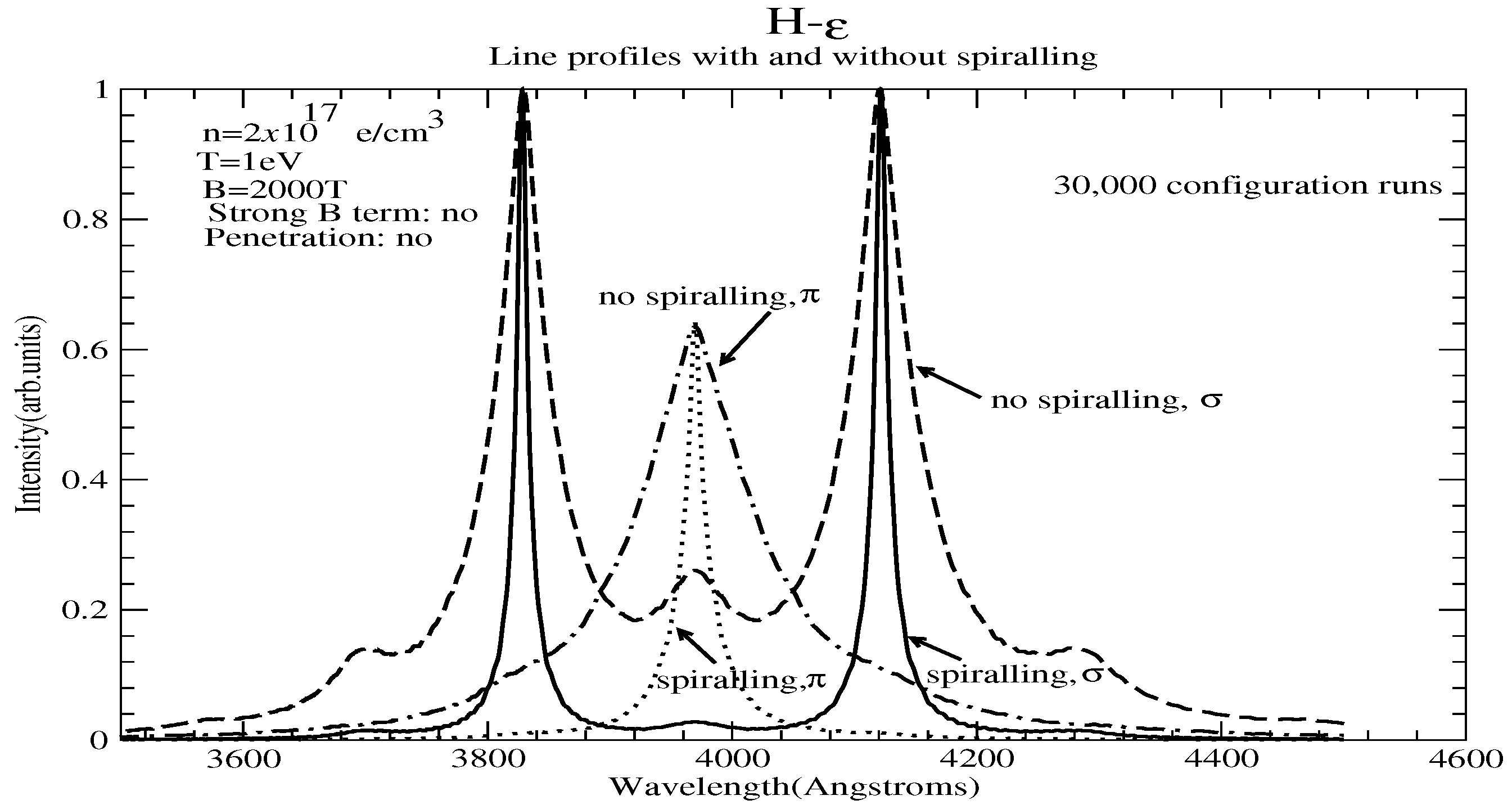
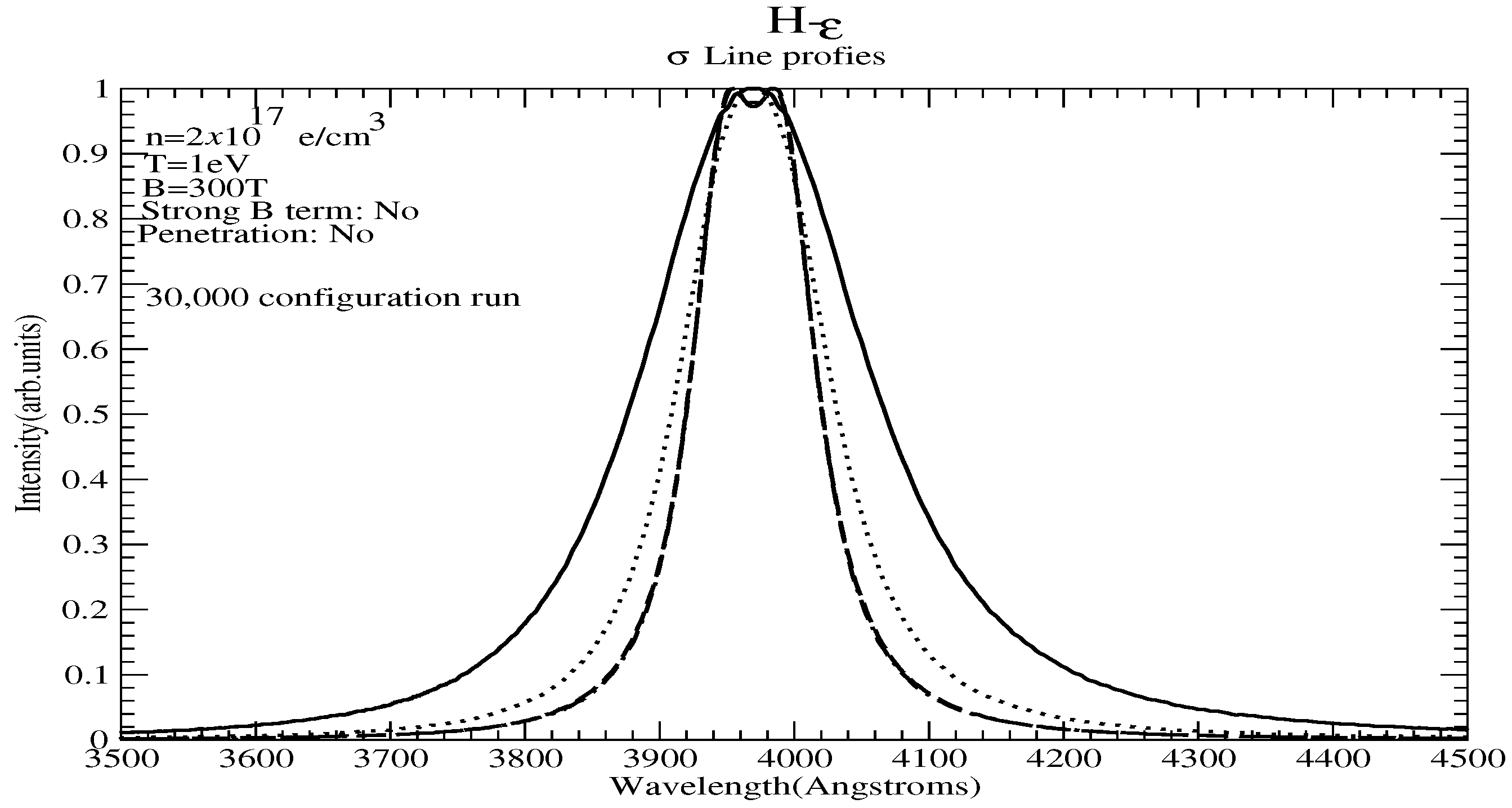
Figure 13, Figure 14 and Figure 15 show the ( and ) profiles with and without spiralling for a magnetic field of 300, 500, and 2000 T, respectively. It is clear that spiralling significantly reduces (instead of enhances, as predicted in [3,4]) the line widths.
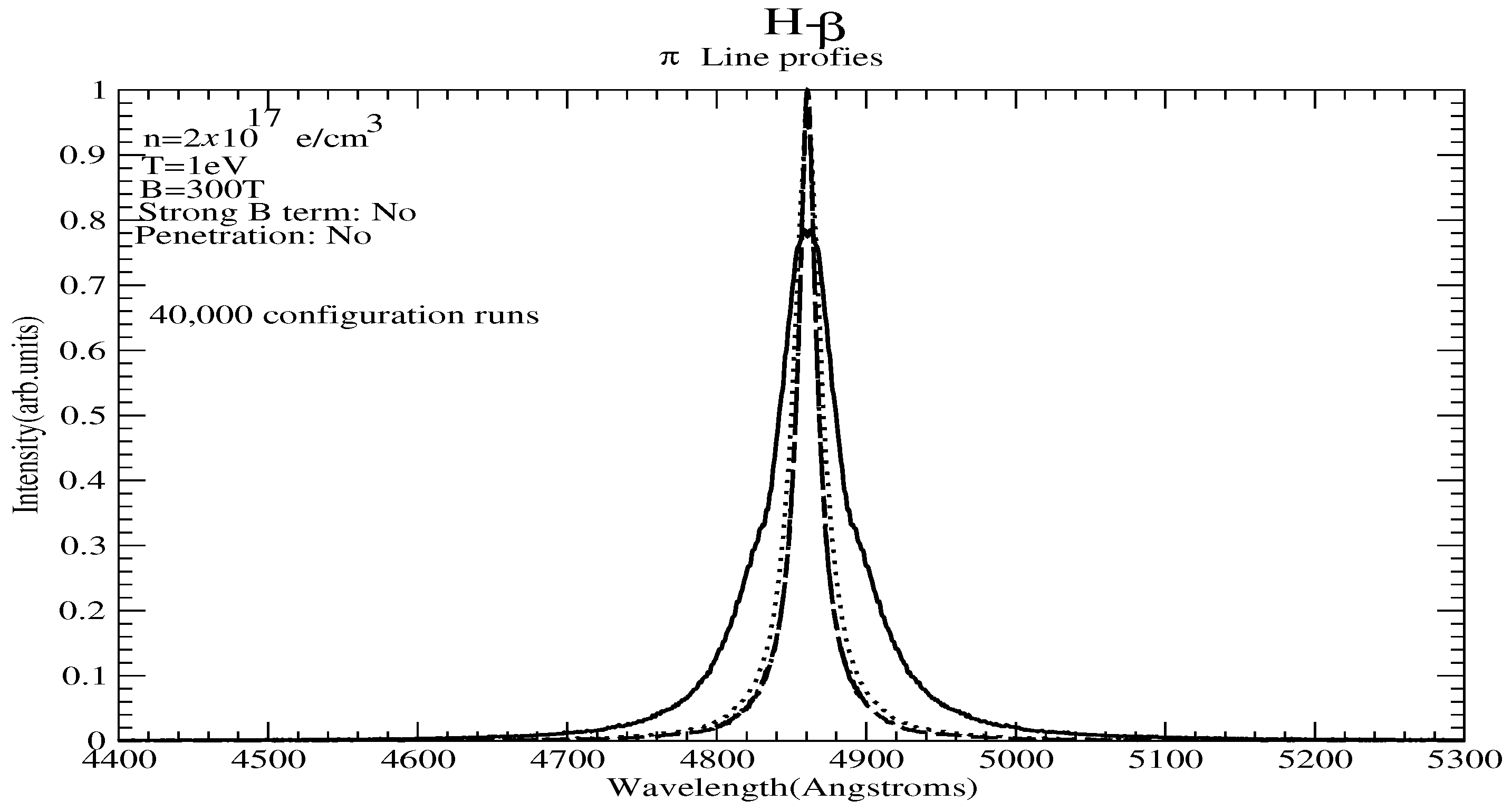
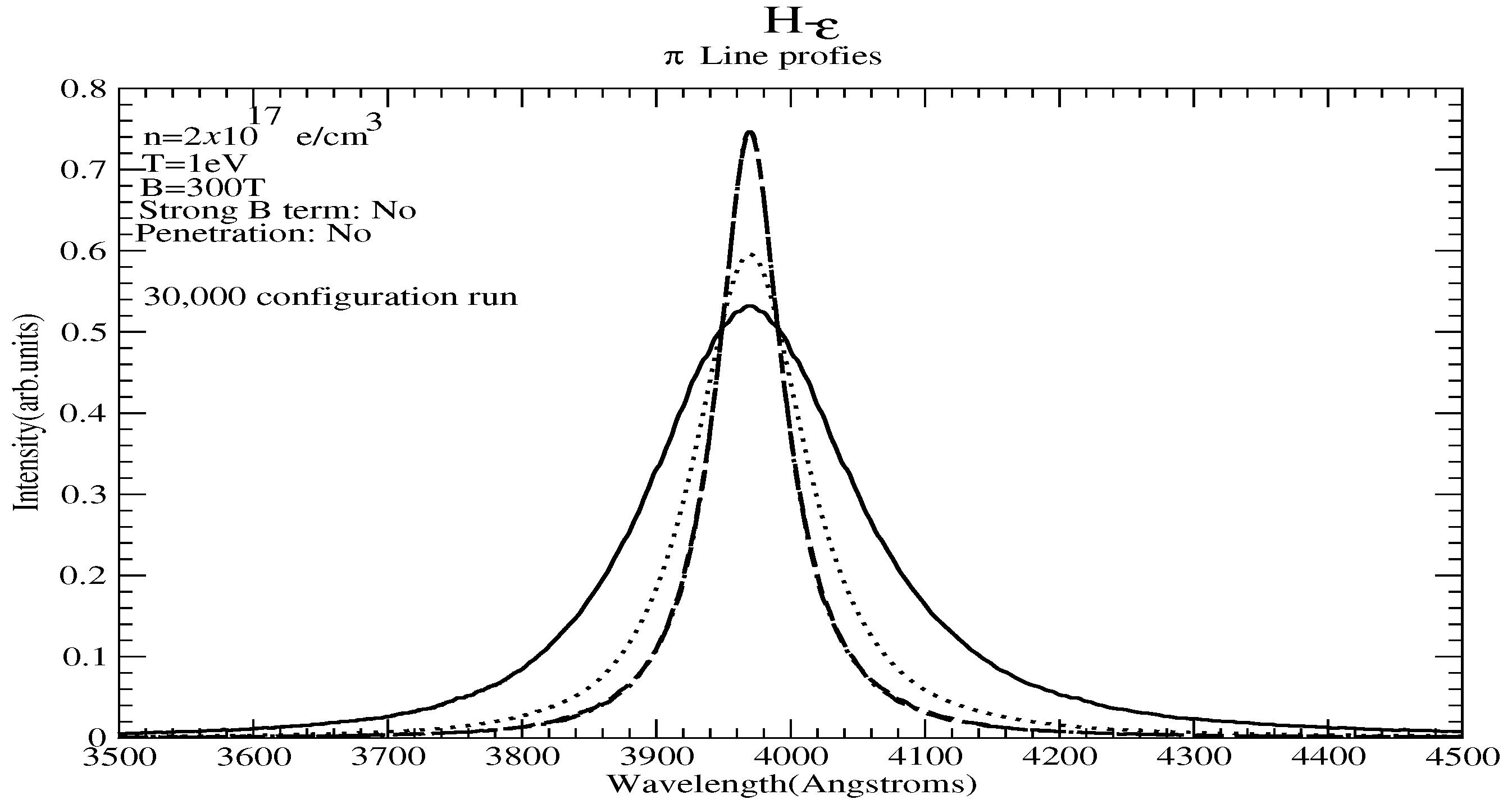
The next task is to consider the effects of electrons and ions on these profiles. We thus show separately for the and components the profiles with and without spiralling and with and without the effects of ion broadening, respectively, which is not a priori considered to be quasistatic. This is conducted for each of the three magnetic fields, i.e., 300 T (Figure 16 and Figure 17 for the and components, respectively), 500 T (Figure 18 and Figure 19 for the and components, respectively), and 2000 T (Figure 20 and Figure 21 for the and components, respectively) separately. The solid line shows the nonspiralling result with electrons and ions, the dotted line shows the nonspiralling result with electrons only, the dashed line shows the spiralling result with electrons and ions, and the dash-dotted line shows the spiralling result with electrons only.
We see that in the spiralling case, ions make no difference (the dashed and dash-dotted lines practically coincide) and that the electronic contribution to the line profile in the nonspiralling case is only slightly larger than the electronic (i.e., total in view of the previous remark) contribution in the spiralling case, again in agreement with the predictions of refs. [13,15]. There are two main qualitative features: First, the fact that the nonspiralling electron conribution is slighty larger than the spiralling one. This is mainly due to the difference between and , since the term dominates [15]. Second, the fact that ion broadening is far more diminished in the spiralling case, which was discussed in the previous section. In all calculations, the time of interest T was 4 ps, during which time, the autocorrelation time had long dropped to negligible levels. In the tables under “Model”, ‘S’ denotes with and ‘NS’ without spiralling. The ratios and are the inverse of q for electrons and ions, using respectively the electron or ion Larmor frequency and reduced mass.
The electron and are in micron (), while the ion counterparts and are in ().
As shown in Table 1, in all cases, when spiralling is accounted for, less electrons contribute compared to the nonspiralling case. Effectively, the “relevant” electron density is smaller, and this is consistent with the smaller electron widths seen for spiralling. The fact that the “relevant” ion density is larger is unimportant here, as the ion contribution is negligible, as already discussed, besides the fact that the ionic contribution is partial, as typically .
4.2. Strong B Effects
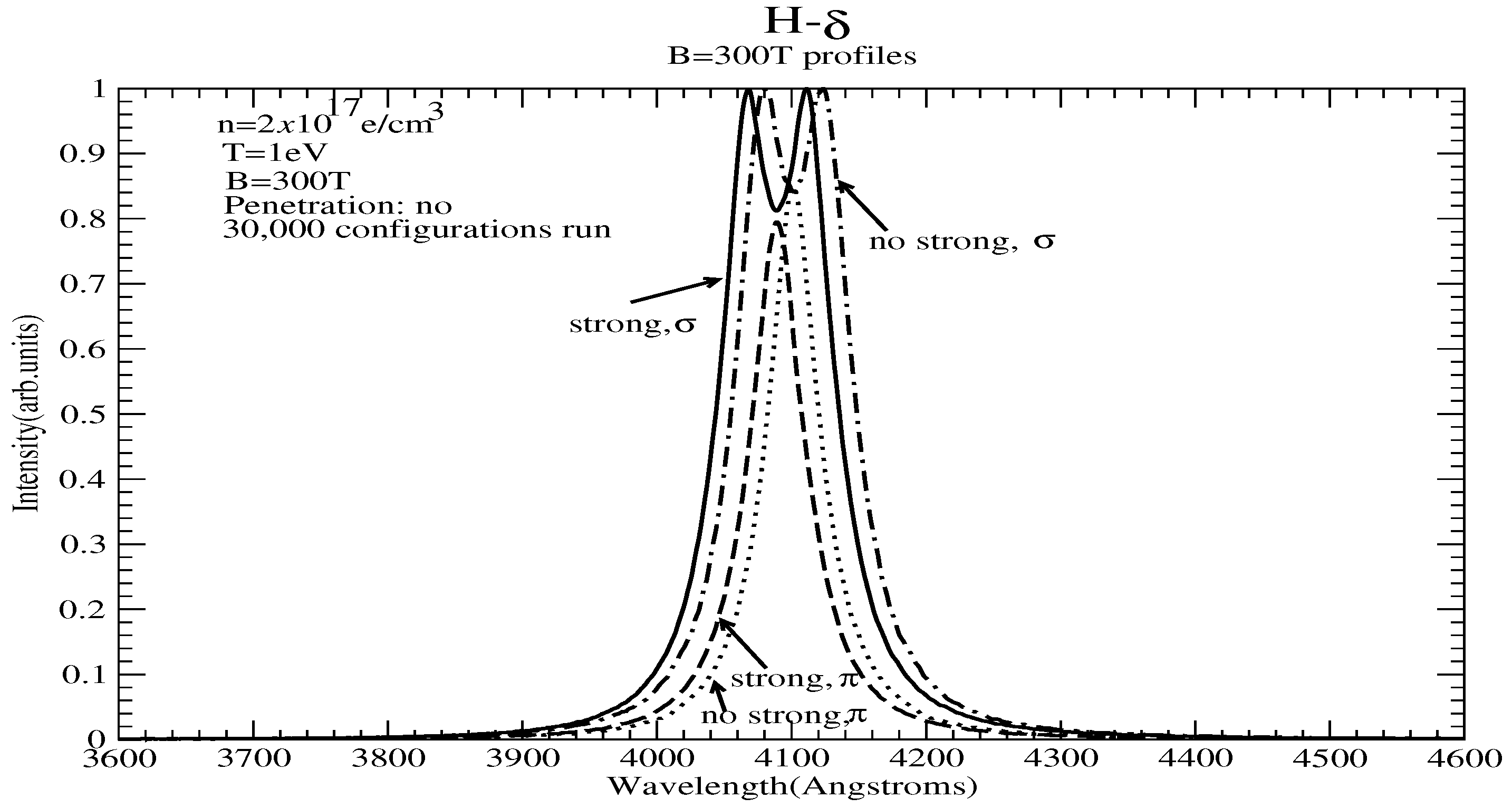
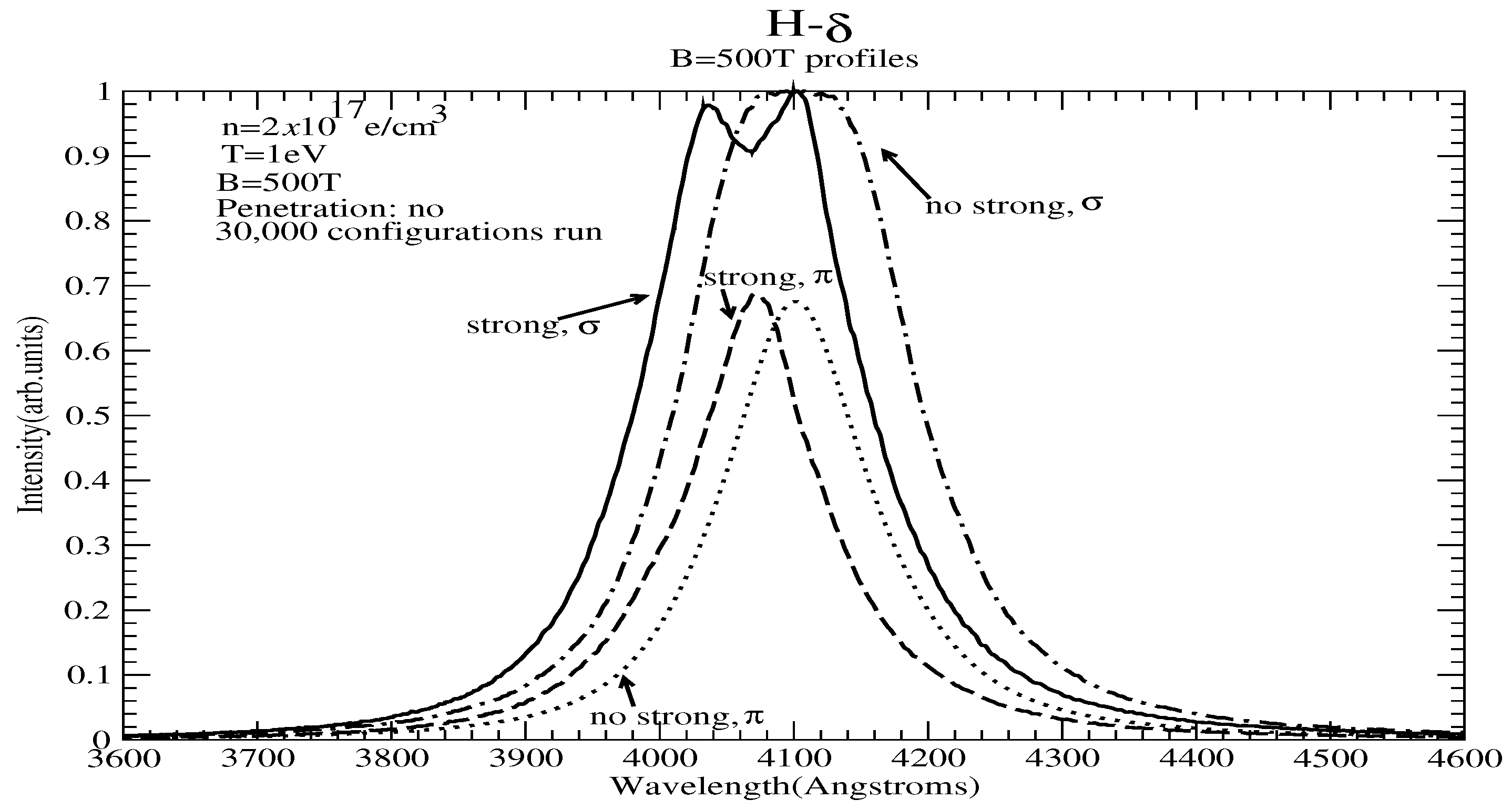
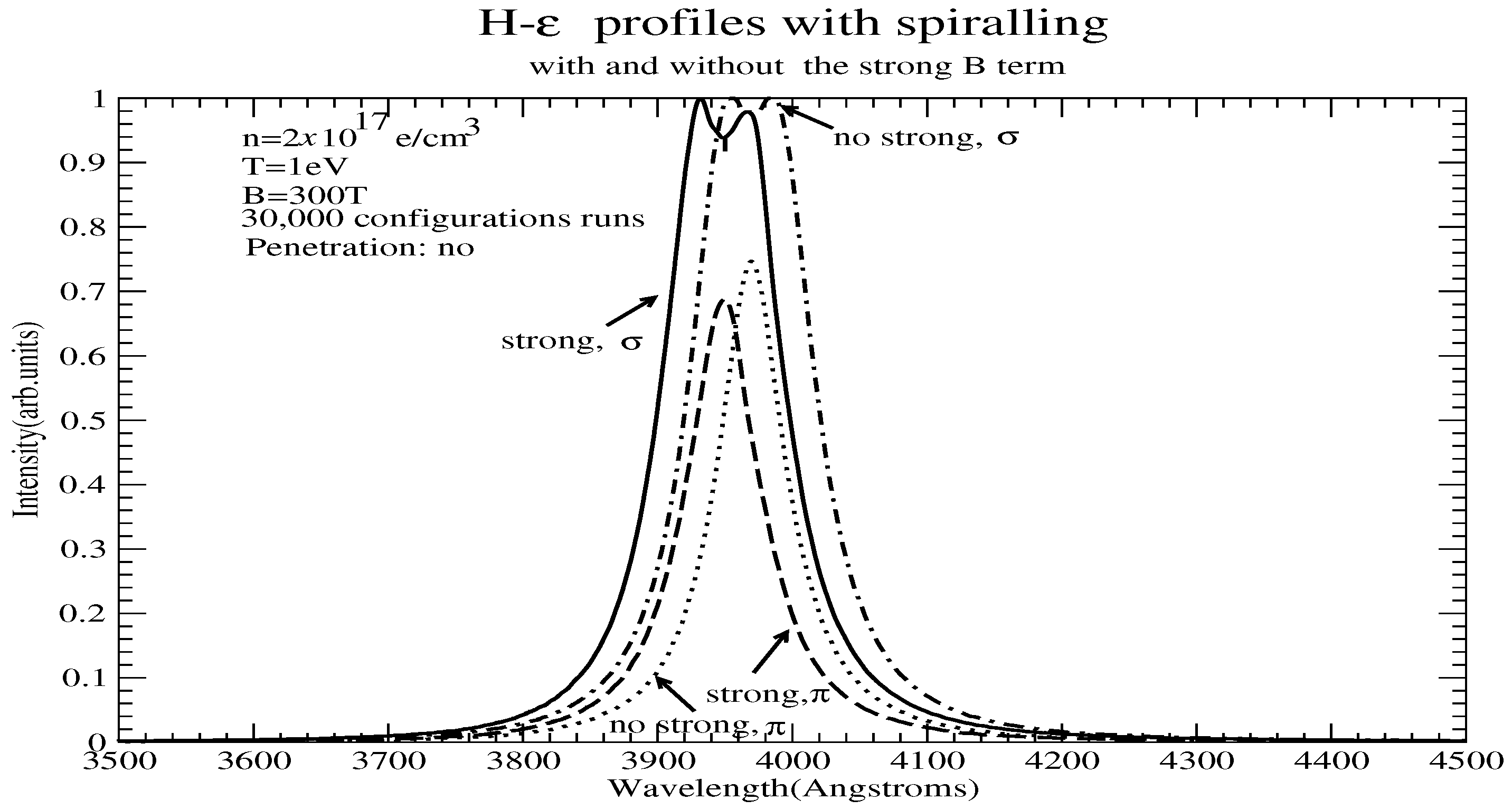
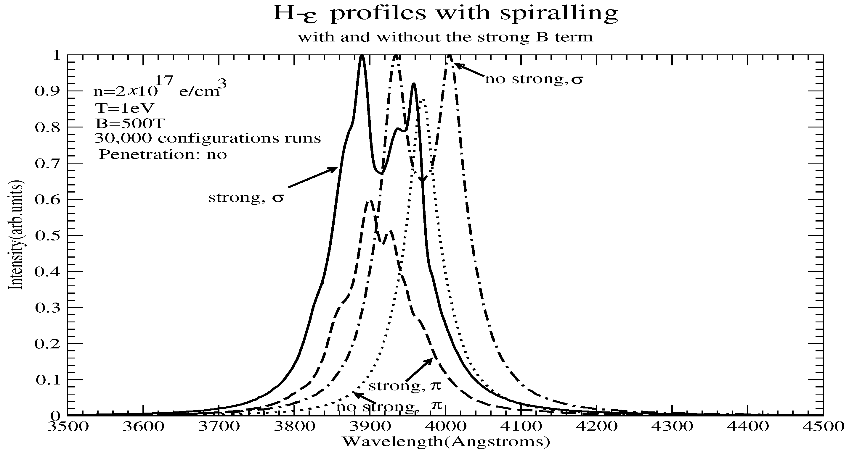
Figure 22, Figure 23 and Figure 24 show the differences in the spiralling calculation when the strong B term is taken into account for B = 300 T, 500 T, and 2000 T, respectively. For B = 300 and 500 T, the effects are very small—essentially a shift of the profile with some slight asymmetry.
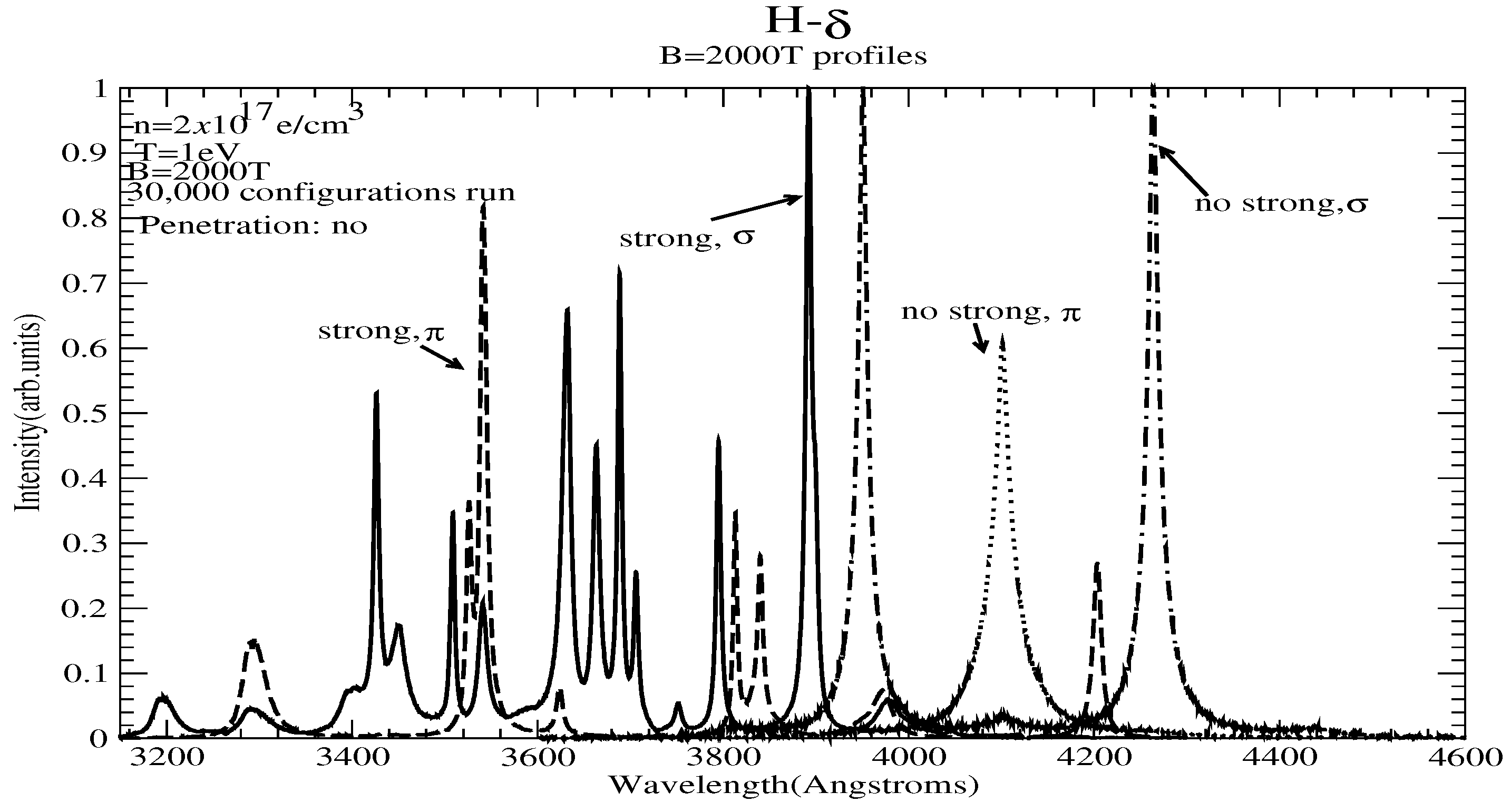
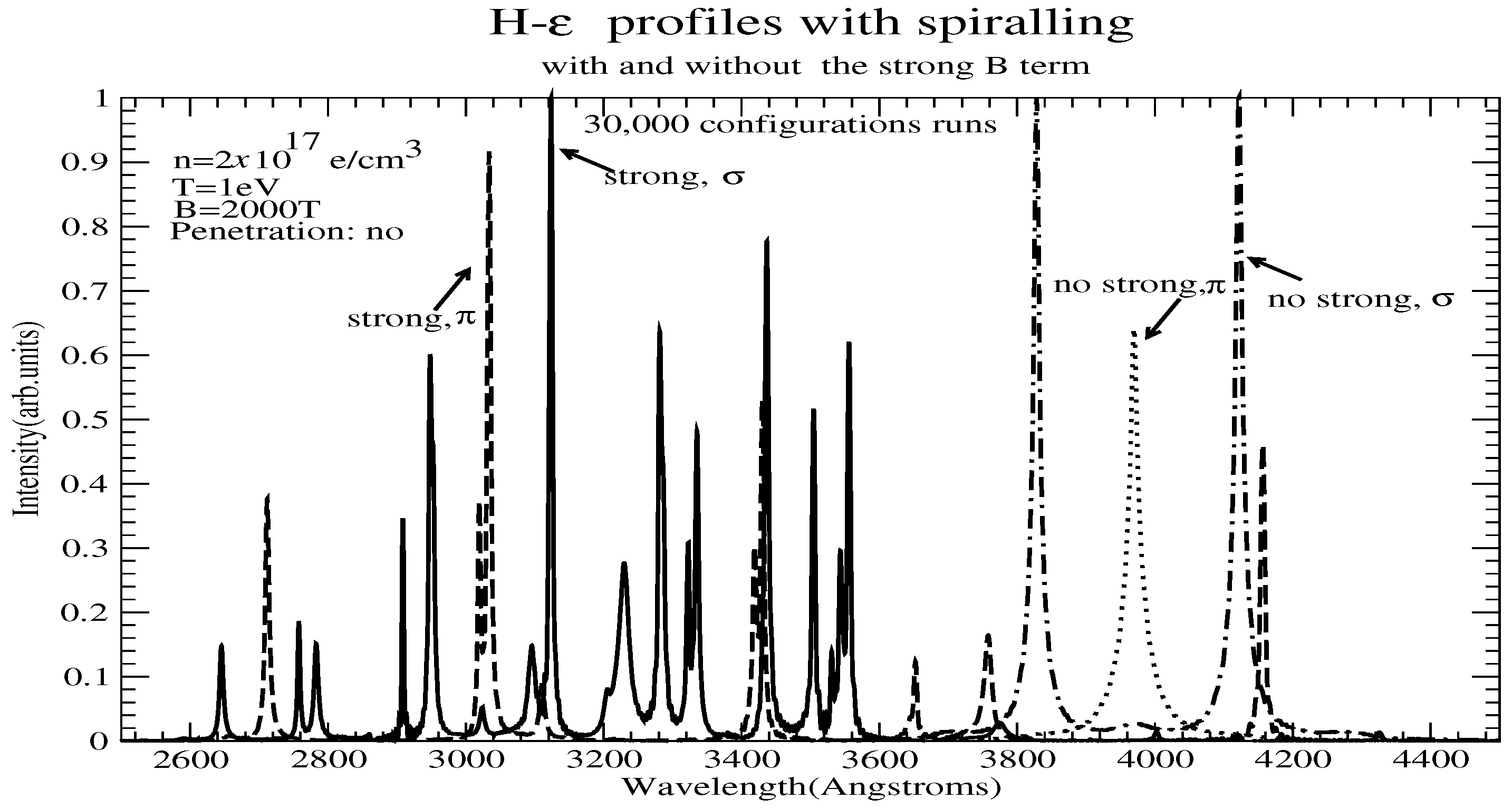
For B = 2000 T, the effects are more significant, with new components being clearly visible. Even for components which appear undisplaced compared to the calculation with the strong B term neglected, intensities and widths are quite different.
5. H- Line
5.1. Profiles without the Strong B-Term
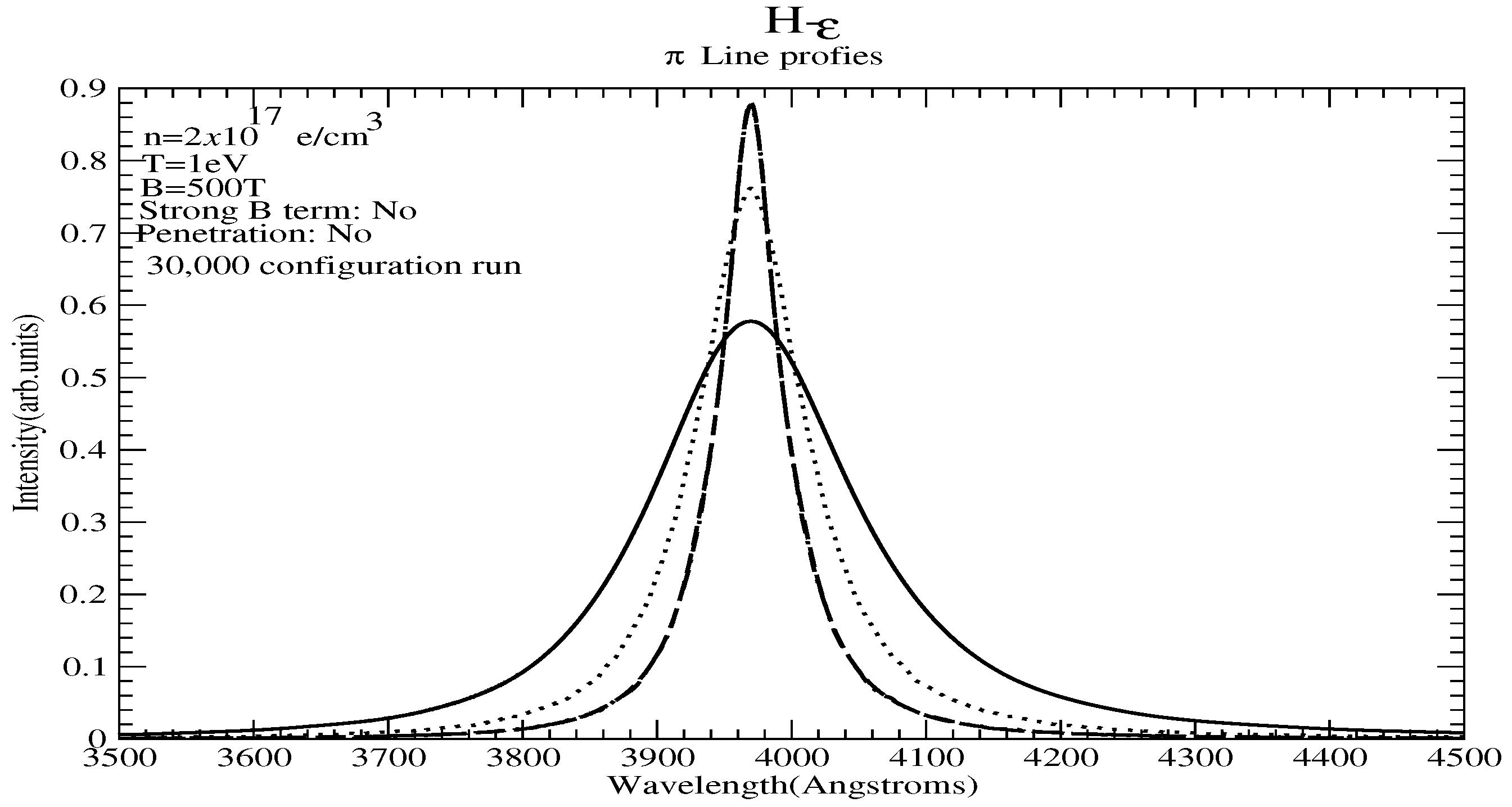
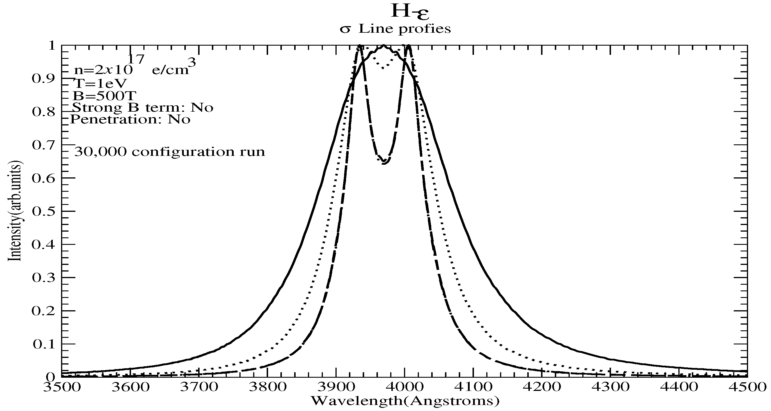
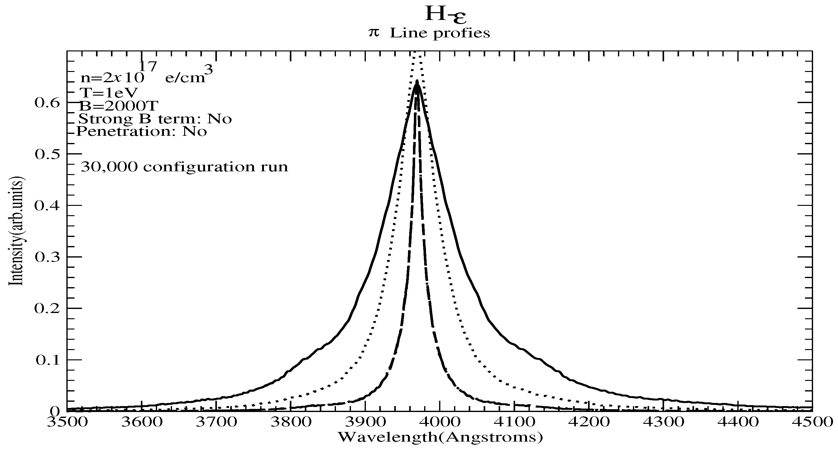
As shown in Figure 25, Figure 26 and Figure 27 for B = 200, 500, and 2000 T, respectively, the H- line shows a similar behaviour with spiralling, resulting in significantly narrower lines. Next, we consider the contributions of electrons and ions separately, as for . We thus show separately for the and components the profiles with and without spiralling and with and without the effects of ion broadening, which is not a priori considered to be quasistatic. This is conducted for each of the three magnetic fields, i.e., 300 T (Figure 28 and Figure 29 for the and components, respectively), 500 T (Figure 30 and Figure 31 for the and components, respectively), and 2000 T (Figure 32 and Figure 33 for the and components, respectively) separately. The solid line shows the nonspiralling result with electrons and ions, the dotted line shows the nonspiralling result with electrons only, the dashed line shows the spiralling result with electrons and ions, and the dash-dotted line shows the spiralling result with electrons only (which practically is identical to the dashed line with spiralling electrons alone). Once again, in all cases, the same qualitative behaviour is seen as for : electrons dominate ions and the ionic contribution with spiralling accounted for is much smaller than the ionic contribution without spiralling accounted for. Table 2 shows the same qualitative behaviour as that for : when spiralling is accounted for, less electrons contribute compared to the nonspiralling case, while for ions, the opposite holds true. However, the ionic contribution is only partial and always negligible. The term dominates for electron broadening, whereas for ion broadening, it is comparable or smaller than .
5.2. Strong B Effects
Figure 34, Figure 35 and Figure 36 show the differences in the spiralling calculation when the strong B term is taken into account for B = 300 T, 500 T, and 2000 T, respectively. The same qualitative conclusions apply as for : For B = 300 and 500 T, the effects are very small, essentially a shift of the profile with some slight asymmetry, while for B = 2000 T, we have much stronger effects, resulting in a complete renormalization and new components. Again, we see substantial differences in the intensities and widths even for components that appear undisplaced with respect to the calculations without the strong B term.
6. H- Line
6.1. Profiles without the Strong B-Term
Again, for , as shown in Figure 37, Figure 38 and Figure 39 for B = 300, 500, and 2000 T, respectively, we see a similar behaviour with spiralling, resulting in significantly narrower lines.
Regarding the effects of electrons and ions on these profiles, we show separately for the and components, the profiles with and without spiralling and with and without the effects of ion broadening, which is not a priori considered to be quasistatic. This is conducted for each of the three magnetic fields, i.e., 300 T (Figure 40 and Figure 41 for the and components, respectively), 500 T (Figure 42 and Figure 43 for the and components, respectively), and 2000 T (Figure 44 and Figure 45 for the and components, respectively) separately. The solid line shows the nonspiralling result with electrons and ions, the dotted line shows the nonspiralling result with electrons only, the dashed line shows the spiralling result with electrons and ions, and the dash-dotted line shows the spiralling result with electrons only. Once again, the same qualitative results are obtained, resulting in a reduction in the widths due to spiralling trajectories.
6.2. Strong B Effects
Figure 46, Figure 47 and Figure 48 show the differences in the spiralling calculation, when the strong B term is taken into account for B = 300 T, 500 T, and 2000 T, respectively. As expected, the onset of “significant differences” occurs at smaller B fields, due to the higher polarizability of the n = 7 level. Thus, although for B = 300 T, we have essentially a shift of the profiles, already at B = 500 T, we have, apart from the shift, a visible asymmetry setting in. Once again, even for components that are essentially in the same position when calculated with and without the account of the strong B term, the intensities and widths are quite different.
As expected, for B = 2000 T, the effects are even more significant.
6.3. B-Dependence of Widths
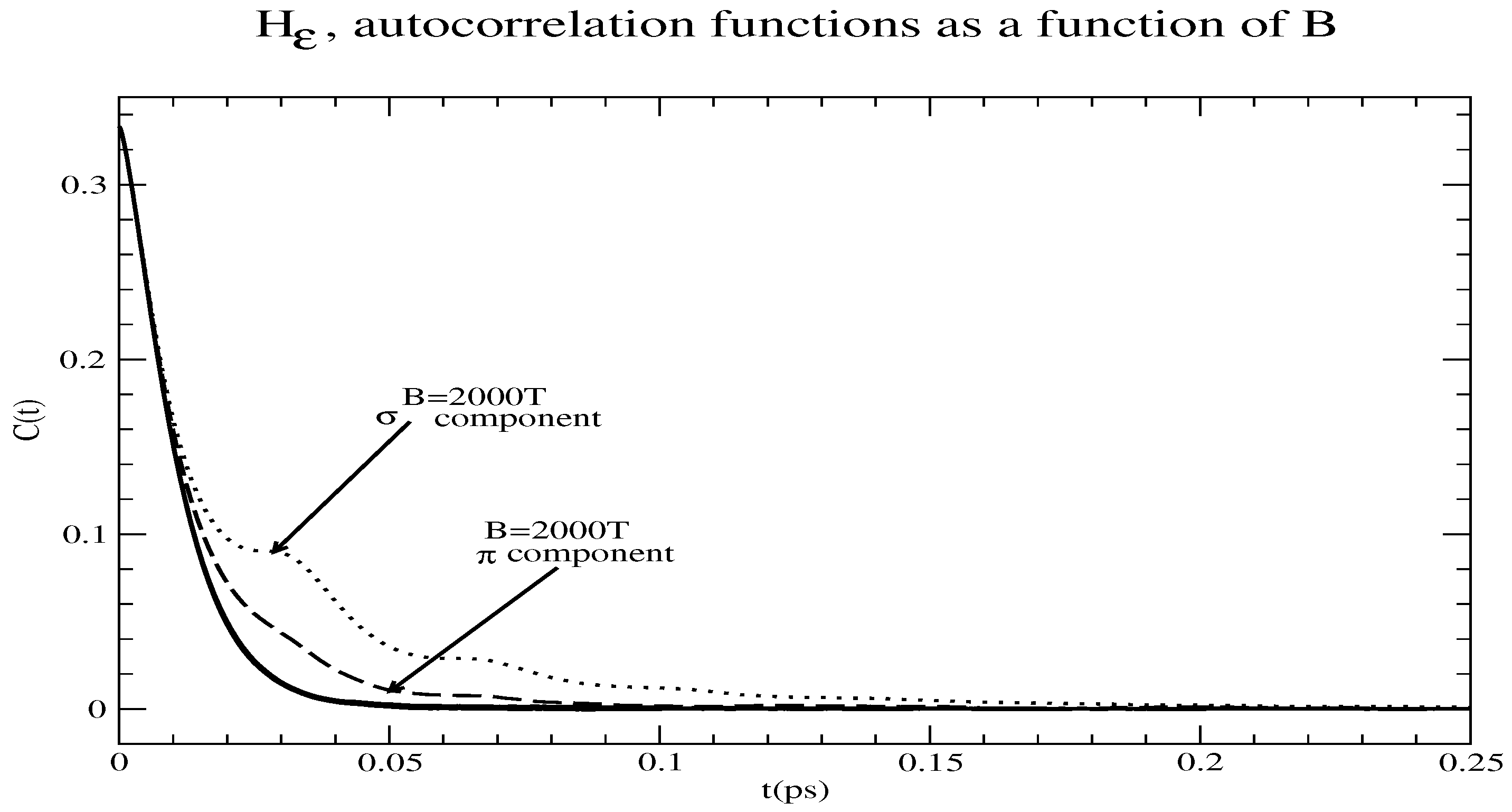
A comparison of widths (allowing spiralling, but neglecting the strong B term) is difficult, because of the overlap of Zeeman components for large B. Instead, we plot the autocorrelation functions (the Fourier transforms of the profiles) of the Zeeman components. Hence, Figure 49 shows the autocorrelation functions of the line components. For B = 0, we have, of course, a single autocorrelation function, and for , the and components’ autocorrelation functions practically coincide, and both are the same regardless of B. However, for B = 2000 T, these are distinctly different and exhibit a slower decay (and hence smaller widths) than the smaller B.
7. Conclusions
A study of the effect of magnetic fields and their effect on line spectra of Rydberg–Balmer lines has been presented, accounting rigorously for both spiralling trajectories and strong magnetic field effects. The results are as follows: First, ion broadening is significantly reduced due to linear Zeeman splitting, resulting in electron broadening dominating these lines. Furthermore, the nonadiabatic contribution is typically negligible; however, strong B effects may produce components with small energy separations from perturbing states, for which the nonadiabatic contribution may be quite important. Second, spiralling further reduces the ionic contribution. Third, spiralling reduces the line widths, typically by small to modest amounts for the parameter range considered. Fourth, correctly accounting for shielding is critical and its neglect can seriously overestimate the widths. Lastly, an interesting question that is outside the scope of the present work is the behaviour of widths on the B-field for small, but nonzero magnetic fields, where for both electrons and ions: .
Note added in proof: After the paper was submitted, the work of ref. [17] has come to our attention. This work deals with a much larger magnetic field that is considered here (and higher densities), and as a result, with quite small Larmor radii. In addition, penetrating collisions are taken into account in that work, whereas they are not taken into account here, as discussed. The authors also find that for their parameter range, screening makes a small difference, which is not the case here. The authors argue that the spiralling electrons should be treated quantum-mechanically and find that broadening is enhanced. The authors “believe that this increase in the line widths is solely a consequence of a quantum-mechanical treatment of the perturbing electrons and the density matrix”. As a result, the present work is not comparable to ref. [17], but it is comparable to [3,4,5]. A detailed comparison, both for cases where agreement is expected and where disagreement should be likely, with ref. [17] is being planned for the next Spectral Line Shapes (SLSP) Workshop. Note that the results of ref. [17] are for the Lyman line, for which refs. [3,4,5] predict that accounting for spiralling trajectories will result in a reduced broadening.
Funding
This research received no external funding.
Data Availability Statement
Raw data are available from the author.
Acknowledgments
The author gratefully aknowledges discussions on ref. [17] with T. Gomez.
Conflicts of Interest
The author declares no conflict of interest.
References
- Rosato, J.; Kieu, N.; Meireni, M.; Koubiti, M.; Marandet, Y.; Stamm, R.; Kovacević-Dojcinovic, J.; Dimitrijevic, M.S.; Popovic, L.C.; Simic, Z. A new analysis of spectral line shapes in white dwarf atmospheres. J. Phys. Conf. Ser. 2019, 1289, 012006–012008. [Google Scholar] [CrossRef]
- Rosato, J.; Kieu, N.; Hannachi, I.; Koubiti, M.; Marandet, Y.; Stamm, R.; Dimitrijevic, M.S.; Simic, Z. Stark-Zeeman Line Shape Modeling for Magnetic White Dwarf and Tokamak Edge. Atoms 2017, 5, 36–45. [Google Scholar] [CrossRef]
- Oks, E. Latest advances in the semiclassical theory of the Stark broadening of spectral lines in plasmas. J. Phys. Conf. Ser. 2017, 810, 012006–012012. [Google Scholar] [CrossRef]
- Oks, E.; Dalimier, E.; Angelo, P.; Sanders, P. Review of recent advances in the analytical theory of Stark broadening of spectral lines in plasmas: Applications to laboratory discharges and astrophysical plasmas. J. Phys. Conf. Ser. 2023, 2439, 012009–012015. [Google Scholar] [CrossRef]
- Oks, E. Effect of Helical Trajectories of Electrons in Strongly Magnetized Plasmas on the Width of Hydrogen/Deuterium Spectral Lines: Analytical Results and Applications to White Dwarfs. Int. Rev. At. Mol. Phys. 2017, 8, 61–72. [Google Scholar]
- Oks, E. Influence of magnetic-field-caused modifications of trajectories of plasma electrons on spectral line shapes: Applications to magnetic fusion and white dwarfs. S. Quant. Spectrosc. Radiat. Transf. 2016, 171, 15–27. [Google Scholar] [CrossRef]
- Griem, H.R.; Halenka, J.; Olchawa, W. Comparison of hydrogen Balmer-alpha Stark profiles measured at high electron densities with theoretical results. J. Phys. At. Mol. Opt. Phys. 2005, 38, 975. [Google Scholar] [CrossRef]
- Alexiou, S.; Griem, H.R.; Halenka, J.; Olchawa, W. A critical analysis of the advanced generalized theory: Applicability and applications. J. Quant. Spectrosc. Radiat. Transfer. 2006, 99, 238. [Google Scholar] [CrossRef]
- Stambulchik, E.; Alexiou, S.; Griem, H.R.; Kepple, P. Stark broadening of high principal quantum number hydrogen Balmer lines in low-density laboratory plasmas. Phys. Rev. E 2007, 75, 016401. [Google Scholar] [CrossRef] [PubMed]
- Alexiou, S.; Weingarten, A.; Maron, Y.; Sarfaty, M.; Krasik, Y.E. Novel Spectroscopic Method for Analysis of Nonthermal Electric Fields in Plasmas. Phys. Rev. Lett. 1995, 75, 3126–3129. [Google Scholar] [CrossRef] [PubMed]
- Weingarten, A.; Alexiou, S.; Maron, Y.; Sarfaty, M.; Krasik, Y.E.; Kingsep, Y. Observation of nonthermal turbulent electric fields in a nanosecond plasma opening switch experiment. Phys. Rev. E 1999, 59, 1096–1110. [Google Scholar] [CrossRef]
- Alexiou, S. X-ray laser line narrowing: New developments. J. Quant. Spectrosc. Radiat. Transfer. 2001, 71, 139–146. [Google Scholar] [CrossRef]
- Rosato, J. Hydrogen Line Shapes in Plasmas with Large Magnetic Fields. Atoms 2020, 8, 74. [Google Scholar] [CrossRef]
- Kieu, N.; Rosato, J.; Stamm, R.; Kovačević-Dojcinović, J.; Dimitrijević, M.S.; Popović, L.Č.; Simić, Z. A New Analysis of Stark and Zeeman Effects on Hydrogen Lines in Magnetized DA White Dwarfs. Atoms 2017, 5, 44. [Google Scholar] [CrossRef]
- Alexiou, S. Line Shapes in a Magnetic Field: Trajectory Modifications I: Electrons. Atoms 2019, 7, 52–63. [Google Scholar] [CrossRef]
- Alexiou, S. Line Shapes in a Magnetic Field: Trajectory Modifictions II: Full Collision-Time Statistics. Atoms 2019, 7, 94–104. [Google Scholar] [CrossRef]
- Gomez, T.; Zammit, M.C.; Fontes, C.J.; White, J.R. A Quantum-mechanical Treatment of Electron Broadening in Strong Magnetic Fields. Astrophys. J. 2023, 951, 143. [Google Scholar] [CrossRef]
Figure 1.
Diagonal upper level –matrix elements as a function of time for a single (the same) plasma microfield realization, with and without a magnetic field. The only effect of the magnetic field is assumed to be the linear Zeeman splitting. It is seen that the addition of the magnetic field results in a slower drop of the U-matrix elements.

Figure 2.
calculation with the full plasma microfield (solid) and only its z-component (dashed). The only effect of the magnetic field is assumed to be the linear Zeeman splitting. It is clear that the nonadiabatic component is only a minor correction. Both the and components are shown.
Figure 2.
calculation with the full plasma microfield (solid) and only its z-component (dashed). The only effect of the magnetic field is assumed to be the linear Zeeman splitting. It is clear that the nonadiabatic component is only a minor correction. Both the and components are shown.

Figure 3.
component of the calculation with the full plasma microfield (solid) and only its z-component (dashed). Spiralling trajectories are still not allowed, but the Zeeman effect is included to all orders.
Figure 3.
component of the calculation with the full plasma microfield (solid) and only its z-component (dashed). Spiralling trajectories are still not allowed, but the Zeeman effect is included to all orders.

Figure 4.
component of the calculation with the full plasma microfield (solid) and only its z-component (dashed). Spiralling trajectories are still not allowed, but the Zeeman effect is included to all orders.
Figure 4.
component of the calculation with the full plasma microfield (solid) and only its z-component (dashed). Spiralling trajectories are still not allowed, but the Zeeman effect is included to all orders.

Figure 5.
calculation at , eV for (a) shielded electron and ions at B = 500 T (dashed), (b) unshielded electrons and ions at B = 500 T (dotted), and (c) shielded electrons and ions, but no spiralling (solid).
Figure 5.
calculation at , eV for (a) shielded electron and ions at B = 500 T (dashed), (b) unshielded electrons and ions at B = 500 T (dotted), and (c) shielded electrons and ions, but no spiralling (solid).

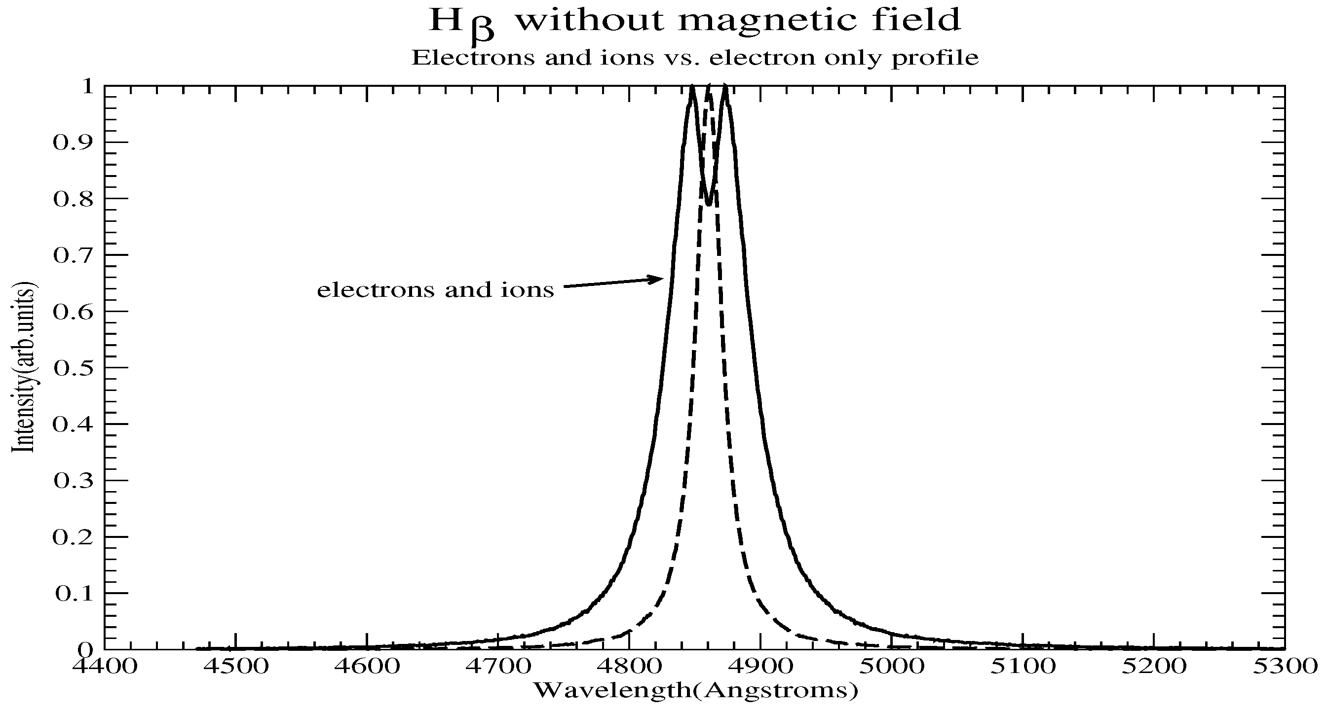
Figure 6.
calculation at , eV, and no magnetic field. Shown are the profiles under the joint action of electrons and ions (solid) and with electron perturbers only (dashed). It is clear that the ion contribution is substantial or even dominant for B = 0.
Figure 6.
calculation at , eV, and no magnetic field. Shown are the profiles under the joint action of electrons and ions (solid) and with electron perturbers only (dashed). It is clear that the ion contribution is substantial or even dominant for B = 0.

Figure 7.
Sample –component of , where is the random ion microfield in the x direction (solid) and (dotted) with the Zeeman splitting.
Figure 7.
Sample –component of , where is the random ion microfield in the x direction (solid) and (dotted) with the Zeeman splitting.

Figure 8.
Four components of the line under a magnetic field of 2000 T with strong magnetic field effects accounted for, but spiralling not accounted for. The dashed line is the B = 0 autocorrelation function. Three of these components (solid) display a sawtooth-like oscillatory behaviour, while the other one does not (dotted).

Figure 9.
Sample component of , with as the random electron microfield in the x direction (solid) and (dotted).
Figure 9.
Sample component of , with as the random electron microfield in the x direction (solid) and (dotted).

Figure 10.
profiles for B = 2000 T without spiralling, but strong B effects accounted for. Shown are the calculations with electrons and ions (solid), only the adiabatic component of electrons and ions (dashed), only electrons (dotted), and only the adiabatic component of electrons (dash-dotted).
Figure 10.
profiles for B = 2000 T without spiralling, but strong B effects accounted for. Shown are the calculations with electrons and ions (solid), only the adiabatic component of electrons and ions (dashed), only electrons (dotted), and only the adiabatic component of electrons (dash-dotted).

Figure 11.
profiles for B = 2000 T without spiralling, but strong B effects accounted for. Shown are the calculations with electrons and ions (solid), only the adiabatic component of electrons and ions (dashed), only electrons (dotted), and only the adiabatic component of electrons (dash-dotted).
Figure 11.
profiles for B = 2000 T without spiralling, but strong B effects accounted for. Shown are the calculations with electrons and ions (solid), only the adiabatic component of electrons and ions (dashed), only electrons (dotted), and only the adiabatic component of electrons (dash-dotted).

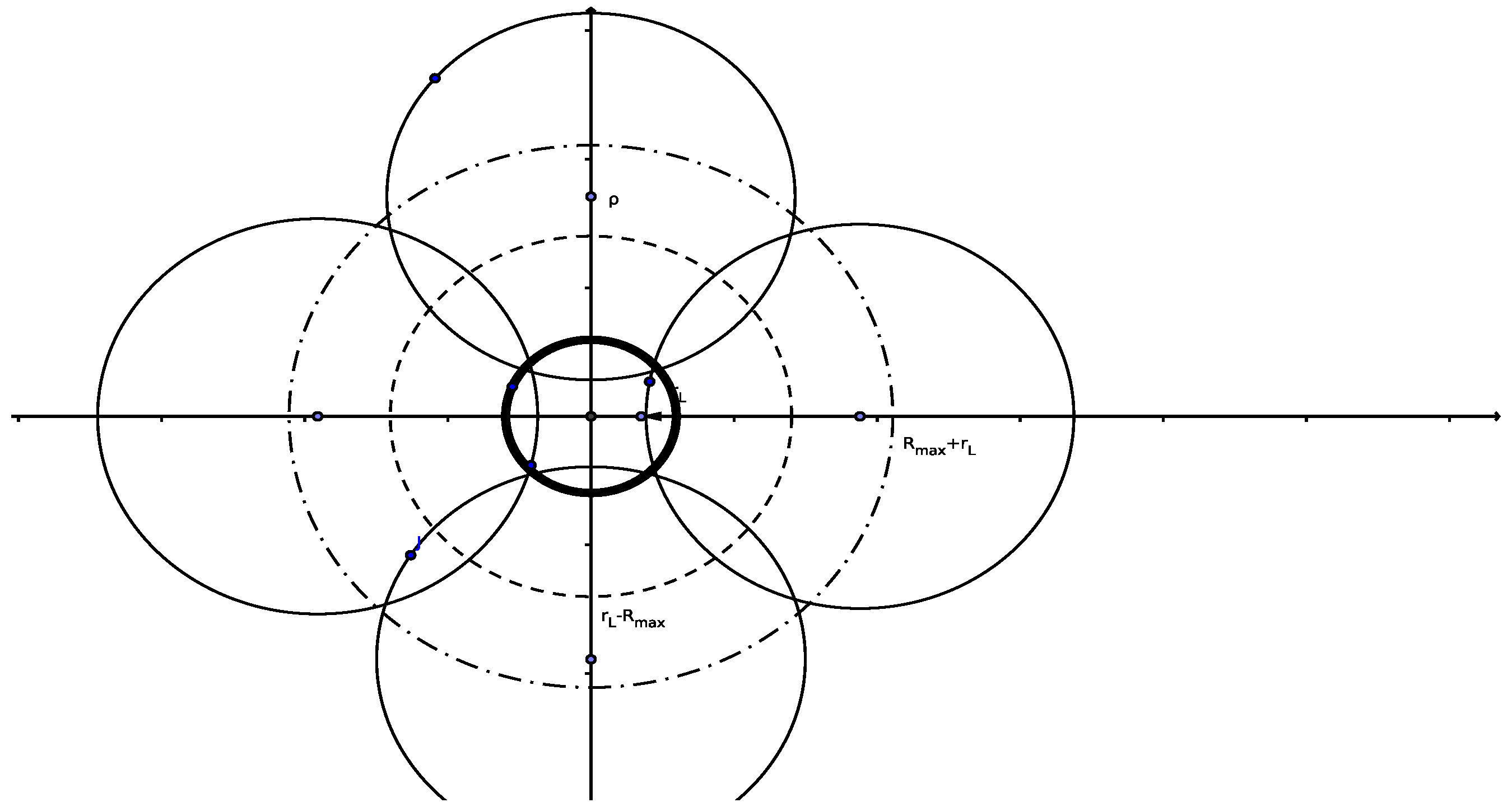
Figure 12.
Typical case for ions, where , so that impact parameters in () contribute, and even these contribute only partially.
Figure 12.
Typical case for ions, where , so that impact parameters in () contribute, and even these contribute only partially.

Figure 13.
and line profiles for the line with and without spiralling and without the strong B term for B = 300 T.
Figure 13.
and line profiles for the line with and without spiralling and without the strong B term for B = 300 T.

Figure 14.
and line profiles for the line with and without spiralling and without the strong B term for B = 500 T.
Figure 14.
and line profiles for the line with and without spiralling and without the strong B term for B = 500 T.

Figure 15.
and line profiles for the line with and without spiralling and without the strong B term for B = 2000 T.
Figure 15.
and line profiles for the line with and without spiralling and without the strong B term for B = 2000 T.

Figure 16.
Comparison of the profiles with and without spiralling for B = 300 T. The strong B term is neglected. Shown are the profiles broadened by nonspiralling electrons and ions (solid), nonspiralling electrons only (dotted), spiralling electrons and ions (dashed), and spiralling electrons only (dash-dotted).

Figure 17.
Comparison of the profiles with and without spiralling for B = 300 T. The strong B term is neglected. Shown are the profiles broadened by nonspiralling electrons and ions (solid), nonspiralling electrons only (dotted), spiralling electrons and ions (dashed), and spiralling electrons only (dash-dotted).

Figure 18.
Comparison of the profiles with and without spiralling for B = 500 T. The strong B term is neglected. Shown are the profiles broadened by nonspiralling electrons and ions (solid), nonspiralling electrons only (dotted), spiralling electrons and ions (dashed), and spiralling electrons only (dash-dotted).

Figure 19.
Comparison of the profiles with and without spiralling for B = 500 T. The strong B term is neglected. Shown are the profiles broadened by nonspiralling electrons and ions (solid), nonspiralling electrons only (dotted), spiralling electrons and ions (dashed), and spiralling electrons only (dash-dotted).

Figure 20.
Comparison of the profiles with and without spiralling for B = 2000 T. The strong B term is neglected. Shown are the profiles broadened by nonspiralling electrons and ions (solid), nonspiralling electrons only (dotted), spiralling electrons and ions (dashed), and spiralling electrons only (dash-dotted).

Figure 21.
Comparison of the profiles with and without spiralling for B = 2000 T. The strong B term is neglected. Shown are the profiles broadened by nonspiralling electrons and ions (solid), nonspiralling electrons only (dotted), spiralling electrons and ions (dashed), and spiralling electrons only (dash-dotted).

Figure 22.
Comparison of spiralling calculations for with and without the account of the strong B-term for B = 300 T. Shown are the profiles with the account of the strong B-term for the (dashed) and (solid) components and without the account of the strong B-term for the (dotted) and (dash-dotted) components.

Figure 23.
Comparison of spiralling calculations for with and without account of the strong B-term for B = 500 T. Shown are the profiles with the account of the strong B-term for the (dashed) and (solid) components and without the account of the strong B-term for the (dotted) and (dash-dotted) components.

Figure 24.
Comparison of spiralling calculations for with and without the account of the strong B-term for B = 2000 T. Shown are the profiles with the account of the strong B-term for the (dashed) and (solid) components and without the account of the strong B-term for the (dotted) and (dash-dotted) components.

Figure 25.
and line profiles for the line with and without spiralling and without the strong B term for B = 300 T. Shown are the profiles broadened by nonspiralling electrons and ions for the (dashed) and (dash-dotted) directions, and by spiralling electrons and ions in the (solid) and (dotted) directions.

Figure 26.
and line profiles for the line with and without spiralling and without the strong B term for B = 500 T. Shown are the profiles broadened by nonspiralling electrons and ions for the (dashed) and (dash-dotted) directions, and by spiralling electrons and ions in the (solid) and (dotted) directions.

Figure 27.
and line profiles for the line with and without spiralling and without the strong B term for B = 2000 T. Shown are the profiles broadened by nonspiralling electrons and ions for the (dash-dotted) and (dotted) directions, and by spiralling electrons and ions in the (solid) and (dashed) directions.

Figure 28.
Comparison of the profiles with and without spiralling for B = 300 T. The strong B term is neglected. Shown are the profiles broadened by nonspiralling electrons and ions (solid), nonspiralling electrons only (dotted), spiralling electrons and ions (dashed), and spiralling electrons only (dash-dotted).

Figure 29.
Comparison of the profiles with and without spiralling for B = 300 T. The strong B term is neglected. Shown are the profiles broadened by nonspiralling electrons and ions (solid), nonspiralling electrons only (dotted), spiralling electrons and ions (dashed), and spiralling electrons only (dash-dotted).

Figure 30.
Comparison of the profiles with and without spiralling for B = 500 T. The strong B term is neglected. Shown are the profiles broadened by nonspiralling electrons and ions (solid), nonspiralling electrons only (dotted), spiralling electrons and ions (dashed), and spiralling electrons only (dash-dotted).

Figure 31.
Comparison of the profiles with and without spiralling for B = 500 T. The strong B term is neglected. Shown are the profiles broadened by nonspiralling electrons and ions (solid), nonspiralling electrons only (dotted), spiralling electrons and ions (dashed), and spiralling electrons only (dash-dotted).

Figure 32.
Comparison of the profiles with and without spiralling for B = 2000 T. The strong B term is neglected. Shown are the profiles broadened by nonspiralling electrons and ions (solid), nonspiralling electrons only (dotted), spiralling electrons and ions (dashed), and spiralling electrons only (dash-dotted).

Figure 33.
Comparison of the profiles with and without spiralling for B = 2000 T. The strong B term is neglected. Shown are the profiles broadened by nonspiralling electrons and ions (solid), nonspiralling electrons only (dotted), spiralling electrons and ions (dashed), and spiralling electrons only (dash-dotted).

Figure 34.
Comparison of spiralling calculations for with and without account of the strong B-term for B = 300 T. Shown are the profiles with the account of the strong B-term for the (dashed) and (solid) components and without the account of the strong B-term for the (dotted) and (dash-dotted) components.

Figure 35.
Comparison of spiralling calculations for with and without account of the strong B-term for B = 500 T. Shown are the profiles with the account of the strong B-term for the (dashed) and (solid) components and without the account of the strong B-term for the (dotted) and (dash-dotted) components.

Figure 36.
Comparison of spiralling calculations for with and without account of the strong B-term for B = 2000 T. Shown are the profiles with the account of the strong B-term for the (dashed) and (solid) components and without the account of the strong B-term for the (dotted) and (dash-dotted) components.

Figure 37.
and line profiles for the line with and without spiralling and without the strong B term for B = 300 T. Shown are the profiles broadened by nonspiralling electrons and ions for the (dashed) and (dash-dotted) directions, and by spiralling electrons and ions in the (solid) and (dotted) directions.

Figure 38.
and line profiles for the line with and without spiralling and without the strong B term for B = 500 T. Shown are the profiles broadened by nonspiralling electrons and ions for the (dashed) and (dash-dotted) directions, and by spiralling electrons and ions in the (solid) and (dotted) directions.

Figure 39.
and line profiles for the line with and without spiralling and without the strong B term for B = 2000 T. Shown are the profiles broadened by nonspiralling electrons and ions for the (dashed) and (dash-dotted) directions, and by spiralling electrons and ions in the (solid) and (dotted) directions.

Figure 40.
Comparison of the profiles with and without spiralling for B = 300 T. The strong B term is neglected. Shown are the profiles broadened by nonspiralling electrons and ions (solid), nonspiralling electrons only (dotted), spiralling electrons and ions (dashed), and spiralling electrons only (dash-dotted).

Figure 41.
Comparison of the profiles with and without spiralling for B = 300 T. The strong B term is neglected. Shown are the profiles broadened by nonspiralling electrons and ions (solid), nonspiralling electrons only (dotted), spiralling electrons and ions (dashed), and spiralling electrons only (dash-dotted).

Figure 42.
Comparison of the profiles with and without spiralling for B = 500 T. The strong B term is neglected. Shown are the profiles broadened by nonspiralling electrons and ions (solid), nonspiralling electrons only (dotted), spiralling electrons and ions (dashed), and spiralling electrons only (dash-dotted).

Figure 43.
Comparison of the profiles with and without spiralling for B = 500 T. The strong B term is neglected. Shown are the profiles broadened by nonspiralling electrons and ions (solid), nonspiralling electrons only (dotted), spiralling electrons and ions (dashed), and spiralling electrons only (dash-dotted).

Figure 44.
Comparison of the profiles with and without spiralling for B = 2000 T. The strong B term is neglected. Shown are the profiles broadened by nonspiralling electrons and ions (solid), nonspiralling electrons only (dotted), spiralling electrons and ions (dashed), and spiralling electrons only (dash-dotted).

Figure 45.
Comparison of the profiles with and without spiralling for B = 2000 T. The strong B term is neglected. Shown are the profiles broadened by nonspiralling electrons and ions (solid), nonspiralling electrons only (dotted), spiralling electrons and ions (dashed), and spiralling electrons only (dash-dotted).

Figure 46.
Comparison of spiralling calculations for with and without account of the strong B-term for B = 300 T. Shown are the profiles with the account of the strong B-term for the (dashed) and (solid) components and without the account of the strong B-term for the (dotted) and (dash-dotted) components.

Figure 47.
Comparison of spiralling calculations for with and without the account of the strong B-term for B = 500 T. Shown are the profiles with the account of the strong B-term for the (dashed) and (solid) components and without the account of the strong B-term for the (dotted) and (dash-dotted) components.

Figure 48.
Comparison of spiralling calculations for with and without account of the strong B-term for B = 2000 T. Shown are the profiles with the account of the strong B-term for the (dashed) and (solid) components and without the account of the strong B-term for the (dotted) and (dash-dotted) components.

Figure 49.
autocorrelation functions for B = 0, 300, 500 T (solid), and 2000 T. For the 0, 300, and 500 T, the and components practically coincide. For B = 2000 T, the (dotted) and (dashed) components differ and are shown as such.
Figure 49.
autocorrelation functions for B = 0, 300, 500 T (solid), and 2000 T. For the 0, 300, and 500 T, the and components practically coincide. For B = 2000 T, the (dotted) and (dashed) components differ and are shown as such.


Table 1.
Number of perturbers required for with T = 4 ps.
| B | Model | Electrons | Ions | ||||||
|---|---|---|---|---|---|---|---|---|---|
| 300 | NS | 4827 | 242 | 0.225 | 6.82 | ||||
| 300 | S | 3033 | 272 | 0.225 | 6.82 | ||||
| 500 | NS | 4827 | 242 | 0.135 | 4.1 | ||||
| 500 | S | 2631 | 285 | 0.135 | 4.1 | ||||
| 2000 | NS | 4827 | 242 | 0.03 | 1.02 | ||||
| 2000 | S | 2219 | 464 | 0.03 | 0.9078 |
Table 2.
Number of perturbers required for with T = 3.5 ps.
| B () | Model | Electrons | Ions | ||||||
|---|---|---|---|---|---|---|---|---|---|
| 300 | NS | 3764 | 225 | 0.225 | 6.83 | 1.17 | 0.0332 | 3.865 | 3.32 |
| 300 | S | 2654 | 248 | 0.225 | 6.83 | 0.85 | 3.56 | 4.37 | |
| 500 | NSg | 3764 | 225 | 0.135 | 4.1 | 1.17 | 0.0332 | 3.865 | 3.32 |
| 500 | S | 2302 | 260 | 0.135 | 4.1 | 0.737 | 3.72 | 4.6 | |
| 2000 | NS | 3764 | 225 | 0.0338 | 1.02 | 1.17 | 0.0332 | 3.865 | 3.32 |
| 2000 | S | 1942 | 430 | 0.0338 | 1.02 | 0.62 | 5.51 | 8.23 |
Table 3.
Number of perturbers required for with T = 0.7 ps.
| B () | Model | Electrons | Ions | ||||||
|---|---|---|---|---|---|---|---|---|---|
| 300 | NS | 836 | 128 | 0.225 | 6.83 | 0.773 | |||
| 300 | S | 531 | 151 | 0.225 | 6.83 | 0.17 | |||
| 500 | NS | 836 | 128 | 0.135 | 4.1 | 0.773 | |||
| 500 | S | 460 | 159 | 0.135 | 4.1 | 0.49 | 4.59 | ||
| 2000 | NS | 836 | 128 | 0.0338 | 1.02 | 0.773 | 3.32 | ||
| 2000 | S | 388 | 265 | 0.0338 | 1.02 | 0.868 | 7.6 |
Disclaimer/Publisher’s Note: The statements, opinions and data contained in all publications are solely those of the individual author(s) and contributor(s) and not of MDPI and/or the editor(s). MDPI and/or the editor(s) disclaim responsibility for any injury to people or property resulting from any ideas, methods, instructions or products referred to in the content. |
© 2023 by the author. Licensee MDPI, Basel, Switzerland. This article is an open access article distributed under the terms and conditions of the Creative Commons Attribution (CC BY) license (https://creativecommons.org/licenses/by/4.0/).
Share and Cite
MDPI and ACS Style
Alexiou, S. Effects of Spiralling Trajectories on White Dwarf Spectra: High Rydberg States. Atoms 2023, 11, 141. https://doi.org/10.3390/atoms11110141
AMA Style
Alexiou S. Effects of Spiralling Trajectories on White Dwarf Spectra: High Rydberg States. Atoms. 2023; 11(11):141. https://doi.org/10.3390/atoms11110141
Chicago/Turabian StyleAlexiou, Spiros. 2023. "Effects of Spiralling Trajectories on White Dwarf Spectra: High Rydberg States" Atoms 11, no. 11: 141. https://doi.org/10.3390/atoms11110141
Note that from the first issue of 2016, this journal uses article numbers instead of page numbers. See further details here.