
Review of Rydberg Spectral Line Formation in Plasmas


1
FSUE ≪RFNC-VNIITF Named after Academ E.I. Zababakhin≫, 456770 Snezhinsk, Russia
2
Institute for Laser and Plasma Technologies, National Research Nuclear University MEPhI, 115409 Moscow, Russia
3
Department of Plasma Physics, National Research Centre “Kurchatov Institute”, 123182 Moscow, Russia
*
Author to whom correspondence should be addressed.
Atoms 2023, 11(10), 133; https://doi.org/10.3390/atoms11100133
Submission received: 24 August 2023
/
Revised: 23 September 2023
/
Accepted: 13 October 2023
/
Published: 17 October 2023
(This article belongs to the Special Issue Rydberg Atomic Physics)
Abstract
:The present review is dedicated to the problem of an array of transitions between highly-excited atomic levels. Hydrogen atoms and hydrogen-like ions in plasmas are considered here. The presented methods focus on calculation of spectral line shapes. Fast and simple methods of universal ionic profile calculation for the () and () spectral lines are demonstrated. The universal dipole matrix elements formulas for the and transitions are presented. A fast method for spectral line shape calculations in the presence of an external magnetic field using the formulas for universal dipole matrix elements is proposed. This approach accounts for the Doppler and Stark–Zeeman broadening mechanisms. Ion dynamics effects are treated via the frequency fluctuation model. The accuracy of the presented model is discussed. A comparison of this approach with experimental data and the results of molecular dynamics simulation is demonstrated. The kinetics equation for the populations of highly-excited ionic states is solved in the parabolic representation. The population source associated with dielectronic recombination is considered.
1. Introduction
The hydrogen atom is the simplest quantum system. Both the Schroedinger and the Dirac equations can be solved analytically for an electron in the Coulomb field [1,2,3]. A significant number of works have been dedicated to hydrogen spectra. Nevertheless, there are theoretical issues which are important for plasma spectroscopy problems. For instance, fast calculation of spectral line shapes in magnetized plasma could play a crucial role in divertor plasma diagnostics [4,5]. This task is particularly complicated for transitions from highly excited levels, which are used in certain diagnostic methods [6]. Another example is magnetic field measurements in tokamaks via the Motional Stark Effect [7]. This latter is sensitive to atomic kinetics effects. However, it is a complex task to solve the kinetics equations for highly excited atomic levels;for instance, if the principle quantum number is , then it is necessary to deal with dipole matrix elements [8].
In this paper, we refer to a specific case of the Zeeman effect, namely, the Paschen–Back effect. Thus, we suppose that the energy shift related to the Zeeman effect is mach larger then the fine-structure energy splitting. The description of the Stark and Zeeman effects for hydrogen atoms is natural in parabolic coordinates, as the energy shift in this basis has a simple analytical form [1,3]. Moreover, the combined Stark–Zeeman effect for a hydrogen atom in crossed electric and magnetic fields can be described as the specific basis, which is closely related to the parabolic quantization [9]. Nevertheless, the problem of the Rydberg radiation transition array for large principle quantum numbers n makes numerical calculation of the hydrogen spectra very complex. The number of radiation transitions is proportional to , where n and are the respective principle quantum numbers of the upper and a lower states. However, the radiative transition array for Rydberg atoms can be significantly simplified. Gulayev demonstrated that for large quantum numbers it is possible to neglect radiative transitions [10,11]. Moreover, the expressions for the transition probabilities have a simple form for large n. These results were applied by the authors of the present review to several problems connected with spectral line shape formation and the atomic kinetics of a hydrogen atom (hydrogen-like ion) in plasma. Thus, the purpose of the present paper is to provide the reader with simple analytical solutions of complicated problems which could be used for practical calculations and fast estimations.
In the second section of this paper, we briefly discuss the Stark and Zeeman effects. A universal representation of a spectral line shape for the () and () spectral lines in non-magnetized low-density plasma is presented for in the third section. Simple expressions of the transition probabilities for the hydrogen atom in crossed electric and magnetic fields and applications of these results to spectral line shape calculations are presented in the Section 4. In Section 5, we show how it is possible to obtain simple solutions of the atomic kinetics equations in parabolic coordinates for . A specific case with dielectronic recombination as the population source is considered.
2. Stark and Zeeman Effects: A Brief Overview
The Stark effect in hydrogen atoms (hydrogen-like ions) has a unique feature in that the energy shift of an atom has a non-zero linear term. This fact is connected with the specific symmetry properties of electron wave functions in the Coulomb field [12]. Thus, the energy shift of the hydrogen atom in the external electric field is equal to
where n is the principle quantum number, and are the parabolic quantum numbers, and is the electric quantum number. Note that all expression in this paper are written in their atomic units: , where ℏ is the Planck constant, e is the electron charge, and is the electron mass. The parabolic quantum numbers and the magnetic quantum number m are connected with the principle quantum number
The energy shift for the Zeeman effect is proportional to the magnetic quantum number m:
where B is the magnetic field and is the speed of light in vacuum. Note that we have omitted the term in Formula (3), where is the spin projection, because in the non-relativistic case, which is considered here, the transition probability is proportional to , where is the spin projection of a lower state.
In his famous work [12], Fock investigated the enhanced symmetry of electron wave functions in the Coulomb field. These symmetry properties lead to the existence of the specific basis in which electron states are related to two new motion integrals:
where 1 relates to + and 2 relates to −, is the Runge–Lenz vector, and is the orbital momentum vector. These vectors obey the quantum angular momentum algebra. The parabolic quantum numbers are connected with projections of vectors (4) onto the z axis [13]:
The Hamiltonian of the hydrogen atom in crossed – fields can be represented as
where and are the respective momentum and the coordinate operators of an electron and Z is the charge of the nucleus. The perturbed part can be rewritten in another way:
where
The relation in (9) is valid because in this basis. The energy shift in crossed – fields is equal to
where and are projections of (4) onto the vectors from (9).
Using the angular momentum properties of the vectors in (4), we can express the wave functions in representation in terms of the states:
where is the Wigner d-function:
In (11), are the angles between the vectors and . We choose the reference frame in which the direction of the magnetic field coincides with the z axis:
where is the angle between the electric field and magnetic field .
The dipole matrix elements in the basis from (11) can be written as follows:
where ; here, the intensity of radiation in the dipole approximation is proportional to the squared absolute value of the coordinate matrix element. Calculations of such matrix elements were performed for the first time in [14]. However, the authors of this work considered only the first transitions of the Lyman and Balmer series. The Wigner d-functions can expressed in terms of the Jacobi polynomials [15]:
where , , ,
Generally, there are no selection rules for the parabolic quantum number (, ). However, there are strict selection rules for the magnetic quantum number (). Here, corresponds to the -component of the spectral line (Z-matrix element, the field is parallels to the z axis), and corresponds to the -component (X-matrix element). The accurate formulas for the dipole matrix elements in the parabolic representation were obtained by Gordon [3,16]:
where is the hypergeometric function. Upon the introducing the notation for the first term of the hypergeometric series (18), for the second, etc., we obtain the following:
The Y-matrix element, where and is the azimuth angle, can be obtained using the well known relation . The absolute value of the matrix element X coincides with Y. However, for there is an additional phase for Y-matrix element.
The Gordon Formulas (16) and (17) are very cumbersome. Moreover, the number of terms in the hypergeometric series (18) becomes large with the growth of n. Thus, it is reasonable to use a number of approximate expressions for the Rydberg transitions. The situation becomes more complicated for the probability transition in a Rydberg atom in crossed – fields (14), where it is necessary to calculate () terms in the sum (14) times. Furthermore every term contains four d-functions and complex hypergeometric series. Nevertheless, in the present paper we show how this radiative transition array can be significantly simplified.
3. Stark Broadening of Rydberg Atoms
For the number or radiative transitions grows following . For Rydberg atomic states, the expressions for the transitions probabilities (16) and (17) become very complicated, mostly because of the large number of terms in the series (18). However, in his works [10,11], Gulayev noticed that the last term in the sum (18) is much larger then all the other when . This circumstance allows the Gordon formulas to be simplified. In addition, Gulayev found that the transition probability is very sensitive to the new quantum number K:
The Stark energy shift can be rewritten in terms of the quantum number K:
In the present paper, we consider the () and () spectral lines. For the lines, it is possible to account for the transitions with while neglecting all other transitions. For the component ,
where . The -component for the spectral series corresponds to the central part of the intensity profile.
For the -component ,
where the -component corresponds to the “wings” of a spectral line for the lines.
The conditions for K and set the limitations for the parabolic quantum numbers, leading to existence of the approximate selection rules for the parabolic quantum numbers and . For the component with , and ; for the -component with , and ; for -component with , and ; and for the -component with , and .
For the series, all transitions can be neglected except those with and . The case of corresponds to the -component:
The case of corresponds to -component:
The approximate selection rules are as follows: for and , and ; for and , and . The expressions (25)–(27) are written for the positive values of K. For negative K, it is necessary to switch and . This works for the selections rules as well; both the and components correspond to the wings of the spectral lines, which have a dip in the center.
Note that the transition probabilities in the parabolic basis depend on an absolute value of m. The additional phase in the relation (6) does not influence the atom in an external electric field, as the transition probability is proportional to the absolute value of the squared dipole matrix element. Thus, the description of Stark broadening in non-magnetized plasma can be performed in both the and bases. However, as this phase is important for evaluation of the sum (14), it is important to be careful with the signs when describing the Stark–Zeeman spectra.
The stark shift (linear term) does not depend on the magnetic quantum number m. This opens up the opportunity to perform a simple calculation that derives the expressions which describe the radiation intensity as a function of the energy shift. For the lines:
For the lines:
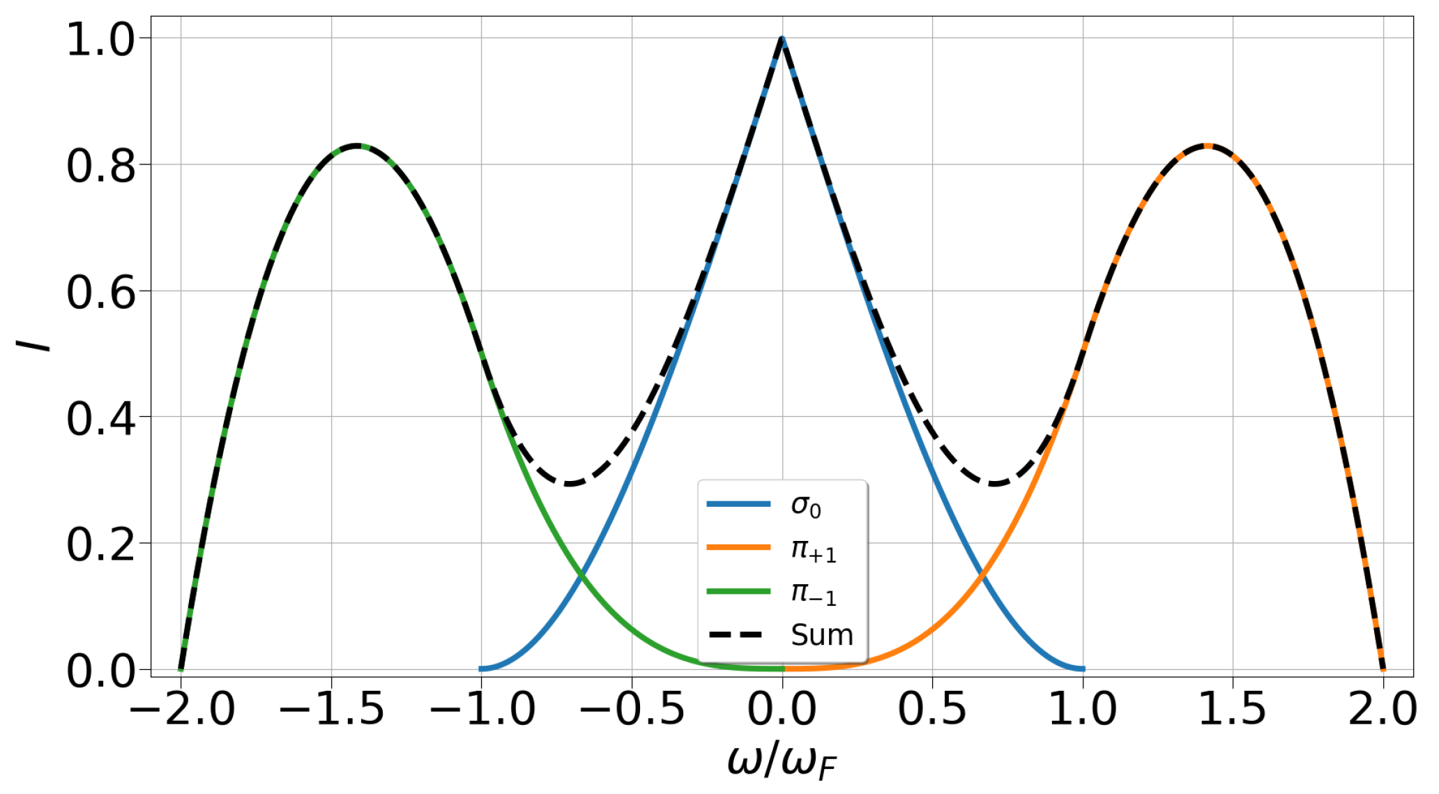
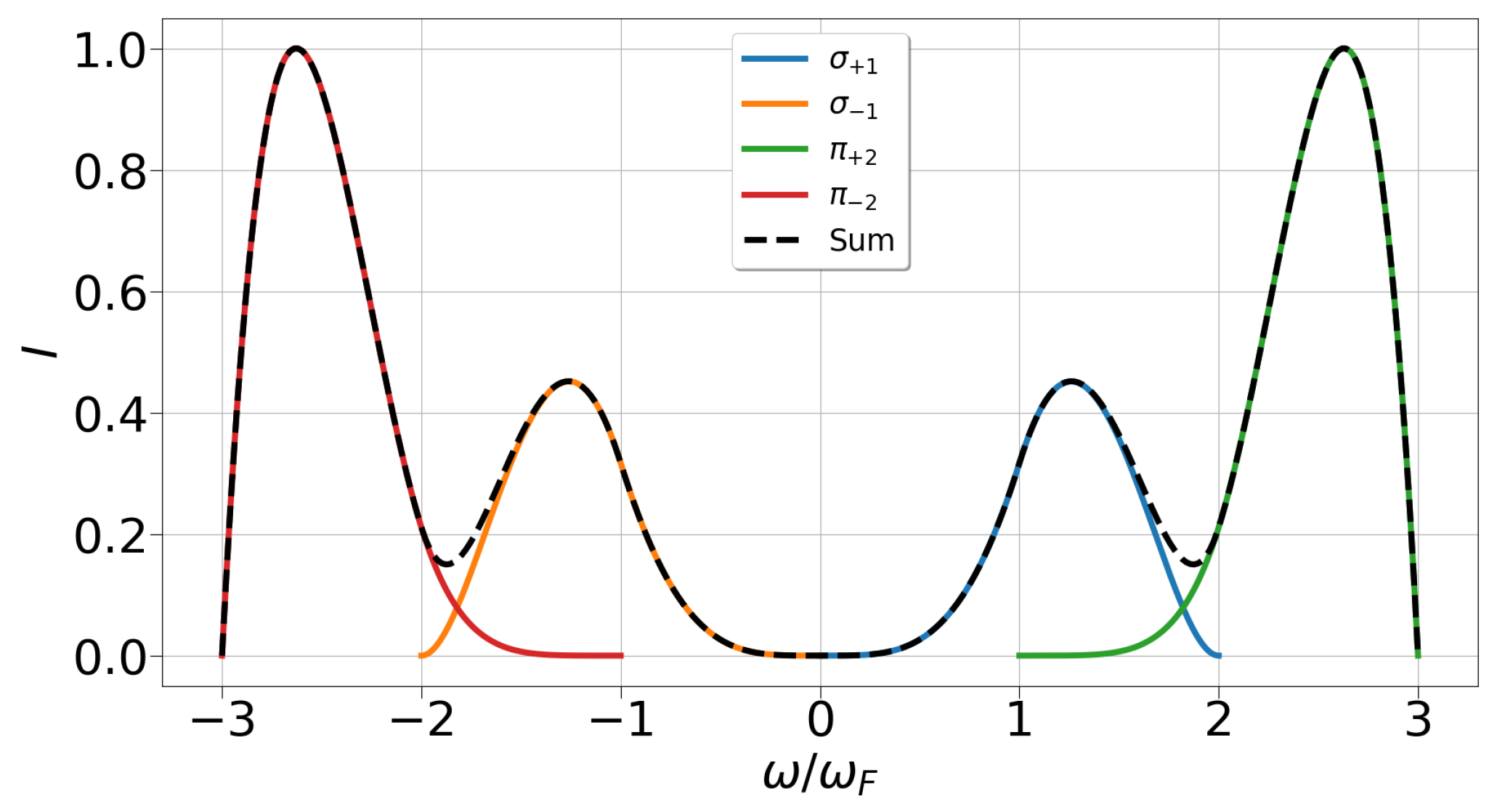
The intensity profiles of the and spectral lines are presented in Figure 1 and Figure 2. The spectral lines have peak in the center and the spectral lines are deep, as expected. Even for a constant electric field, both of these spectral series have a universal representation. It is possible to calculate any line from these series using the scale multiplying factor . However, it is necessary to average these profiles over an electric field distribution to calculate universal representation of spectral lines under Stark broadening. These calculations were performed in [17]. The universal expression for the intensity profile can be represented as follows:
where is the electric field distribution, is the dimensionless electric field, , and . The formulas for can be derived from the expressions (28)–(31):
In the present paper, we consider only low-density plasma, which can be treated as ideal. Thus, we can use the Holtsmark function as the field distribution :
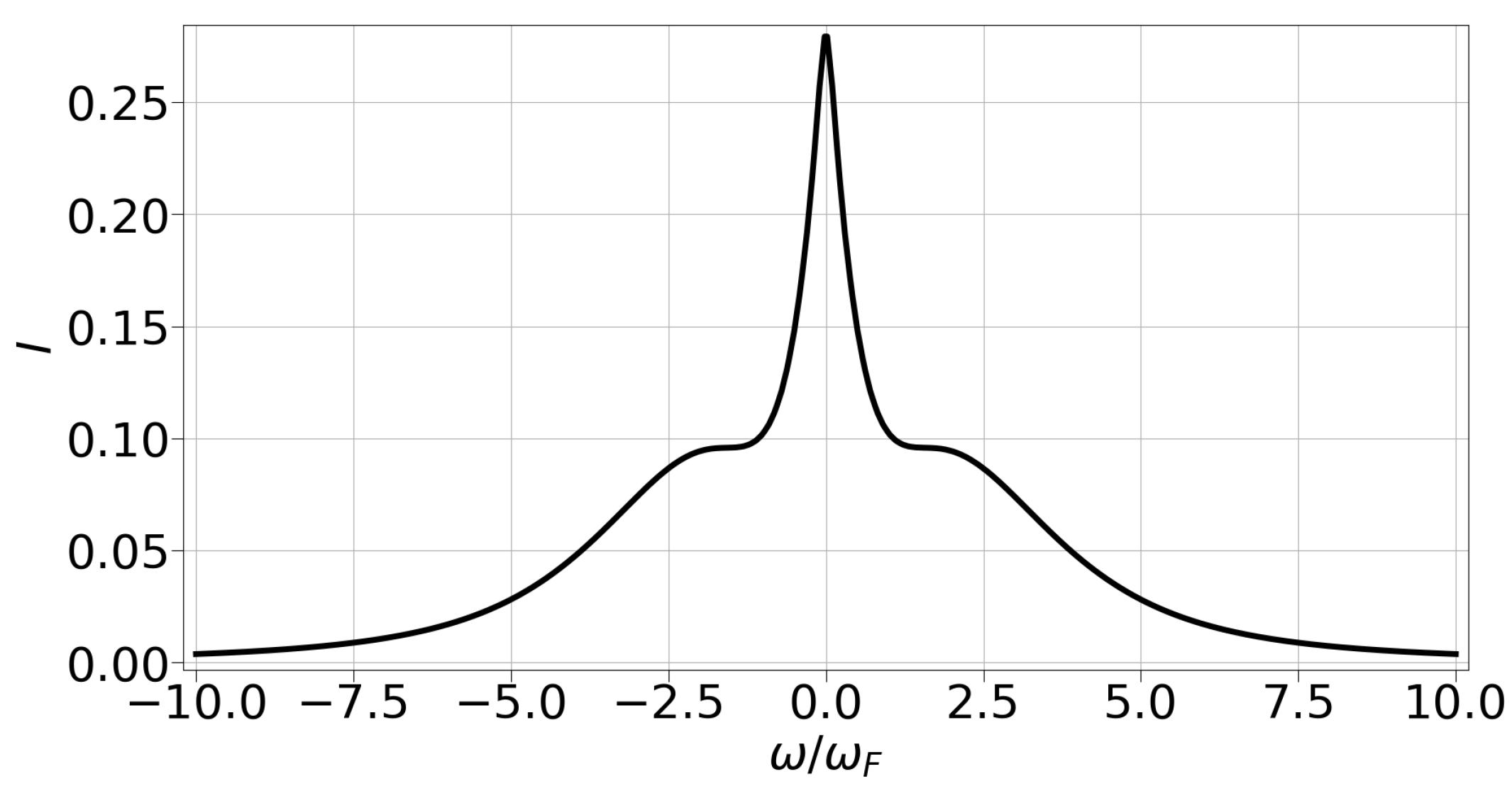
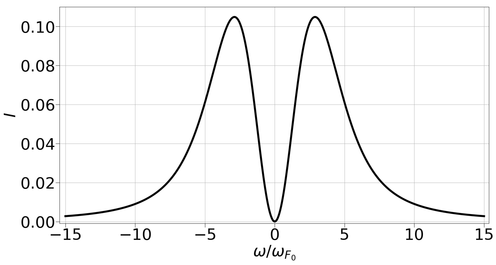
The universal representations of the and spectral line intensity profiles are presented in Figure 3 and Figure 4. This approach works for every line from the corresponding spectral series when . It significantly simplifies calculations, as there is no need to calculate the matrix elements. Note that only quasistatic ion broadening is considered here. To account for the impacts of electron and Doppler broadening mechanisms, it is necessary to calculate the convolution of the function with the Voigt profile.
4. Semiclassical Method of Line Shape Calculation in Magnetized Plasmas
The presence of a magnetic field is common for many plasma devices. Different types of tokamak plasma diagnostics are based on Stark–Zeeman spectral line shape analysis [4,5,6]. However, modeling of such spectra is a very complicated task, as it is necessary to diagonalize the Hamiltonian of an atom in crossed magnetic and fluctuating electric fields. A great deal of theoretical work has been dedicated to this issue [14,18,19,20,21,22,23]. However, these calculation are often hard to reproduce. In [23], the authors suggested a fast and simple algorithm for calculation of spectral line shapes in the presence of an external magnetic field in plasma. This method is based on semiclassical approximation of the expression (14), which has the same form for a constant . The form of these matrix elements does not depend on n, which is why this algorithm is called universal.
The straightforward calculation of the matrix elements (14) is a very complicated issue, especially for Rydberg atomic states. Nevertheless, the expression (14) can be significantly simplified when . It is possible to obtain the universal formulas for the transition probabilities, which have a universal form for every series (fixed ). The Gulayev approach [10,11], discussed above, plays a crucial role in this simplification. The details of the derivation of the simplified dipole matrix elements are presented in [24,25]. For the lines:
For the lines:
Here, can be obtained by switching (which is possible for bar values as well) and in . The same connection exists between and :
It is easy to see that the expressions (38)–(43) have simple structures compare to Formula (14). The derivation of the expressions (38)–(43) is closely related to the specific properties of the Wigner d-functions. The parabolic quantum numbers () obey the approximate selection rules (see the previous section) for a constant value of . It can be helpful to get rid of two sums in (14). The left two sums can be treated separately. Each sum contains two Wigner functions and the factor which corresponds to the dipole matrix element. Using the recurrence relations, the d-function with higher j can be reduced to the sum of two d-functions of order . The coefficients in the recurrence relations coincide with the Gulayev matrix elements. This circumstance allows for use of the orthogonality relation for the d-functions. The latter leads to the presence of the Kronecker’s delta symbols in the expressions (38)–(43). Note that the delta symbols control the addition rules for the angular momentum. The use of the matrix elements (38)–(43) is the key feature of the universal approach. For , it is possible to consider only dipole matrix elements instead of , which significantly simplifies the calculations. Moreover, these expressions have a simple structure and contain only the square roots and trigonometric functions.
We can start with the radiation intensity of an atom in a constant electric field and magnetic field:
where is the full set of all quantum numbers related to the initial and final states, denotes the polarization, defines the angle between the magnetic field and an ion microfield, and is the dipole matrix element. In order to obtain ion static profile, we need to average the expression (44) over the electric microfield:
Formula (46) describes the ionic static profile. However, in a low-density plasma the effects of ion thermal motion might significantly influence the spectral line shape formation. We use the frequency fluctuation model (FFM) [26] to account for the effects of the ion dynamics. The FFM involves the description of stochastic ‘jumps’ between different inhomogeneous spectral components of a line profile. In [27], the authors showed that the complex numerical method necessary to implement the FFM in the spectral line shape calculation algorithm is equivalent to the solution of the kinetics equation for the autocorrelation function with a strong-collisions integral. Thus, complicated numerical calculations can be replaced by the following simple analytical expression:
where and are the concentration and thermal speed of ions, respectively, and is the jumping frequency or the inverse lifetime of a particular value of the microfield. There are other models accounting for ion dynamics effects (see, e.g., [28,29,30]). A cross-comparison between them can be found in [31]. The FFM is chosen to keep this algorithm fast and simple. Here, is the ionic profile which accounts for the ion dynamics effects. In order to evaluate the resulting intensity, it is necessary to account for the impact electron and Doppler broadening mechanisms. To obtain the resulting profile, it is necessary to calculate the convolution of with the Voigt profile :
The expression (51) relates to the Doppler broadening. Here, D is the Doppler parameter
where and and are the respective mass and temperature of the radiators:
The Lorentz distribution (53) corresponds to the electron broadening. Generally, calculating the parameter is a complicated process. Here, we use the simplified approach to electron broadening (see [1]):
where and are the density and thermal velocity of electrons, respectively, and is the Debye radius in the plasma:
where is the coordinate operator and a and b denote different states referring to levels n, , for example,
More accurate calculations of the electron broadening width are discussed in [32].
The convolution of the ionic and Voigt profiles is equal to the resulting intensity profile:
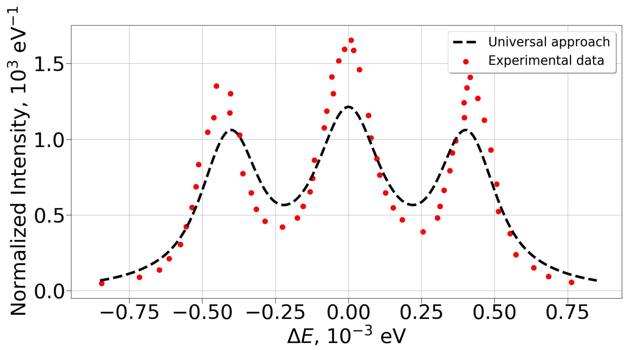
Figure 5 shows a comparison between calculations performed using the method presented in this paper (universal approach) and experimental data from [33] considering the line. These data was obtained as part of the Alcator C-Mod tokamak fusion experiment. The universal approach formally works when . Nevertheless, simple semiclassical calculations reproduce all of the main features of the experimental profile; the experimental line width and location of the triplet peaks are in agreement with the corresponding values obtained through the universal approach. Moreover, we used the simplest models for the microfield distribution, electron impact broadening, and method of accounting for ion dynamics effects. As can be seen from Figure 5, there is satisfactory a correspondence between the experimental datapoints and the theoretical curve.
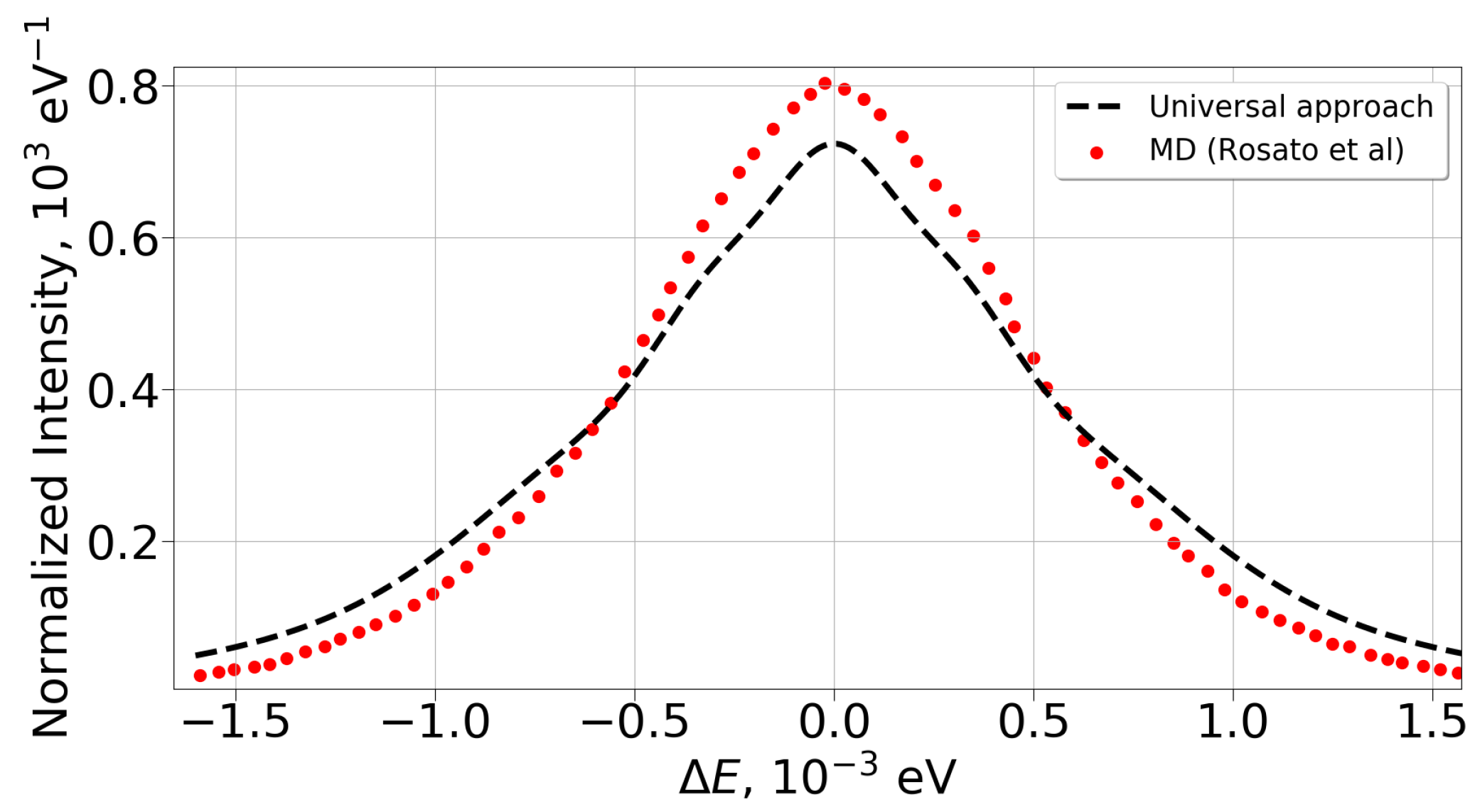
A comparison between the universal approach and the molecular dynamics (MD) simulation results from [20] for line in presented in Figure 6. The line widths, obtained within the universal approach and MD simulation are approximately equal. Also, the there is no triplet for both lines. Again, one can see a good correspondence. So, the universal approach opens the way for fast calculations of spectral line shapes even for the first Balmer lines. It is very important for divertor plasma diagnostics, because one has to do a great number of calculations while fitting experimental profile.
5. Level Population Kinetics for Rydberg Ions
The problem of statistical and dynamical intensities of Stark components is a long-standing issue [3]. If collisions in plasma are frequent enough, then the population of the atomic states is proportional to the corresponding statistical weights. However, if the atomic level radiation decay rate has the same order as the collision frequency, then the so-called dynamical intensities of the Stark components are observed. The description of the Stark splitting is reasonable in the parabolic basis, as already mentioned above. Thus, the kinetics equations for the atomic level must be solved in parabolic coordinates. Here, we face two fundamental problems: the first relates to the description of Rydberg radiation cascade, while the second concerns the need to consider “3D” kinetics equation. Atomic kinetics equations are commonly treated only for the principle quantum numbers n (the 1D case); however, in order to describe the dynamical populations of Stark states, it is necessary to consider all three quantum numbers (the 3D case).
In the present section, we follow the work of [8] and demonstrate the derivation of solutions to atomic kinetics equations for highly excited atomic levels of multi-charged hydrogen-like ions. Dielectronic recombination is considered as the population source for the ionic states. At first, we obtain the applicable area of the method. Here, we consider quasi-static broadening and neglect the ion dynamics effects:
where is the average Stark shift, is the jumping frequency (49), and Z is the average ion’s nucleic charge. The second condition corresponds to the requirement of non-mixing of Stark states for the radiation decay time:
where A is the radiation decay width and is the collision frequency. According to estimations from [8], these demands leads to the following condition for eV:
where is expressed in cm. Using the relation (60), we can obtain the condition for Z:
In [34], the authors obtained the probabilities of radiative transitions between highly excited atomic states in the spherical basis:
where . In order to obtain the kinetics equation in parabolic coordinates, we must turn the expression (62) into its parabolic representation. The connection between the spherical and the parabolic wave functions was obtained by Park [35]:
where is the Clebsch–Gordan coefficient. The straightforward calculation of is a very cumbersome and complex issue. When dealing with large n, it is possible to use the semiclassical approximation for the Clebsch–Gordan coefficients [15]:
where
Using the relation (62) with (64) allows us to derive the expression for the radiation decay probability in the parabolic representation:
Simple evaluation of the integral (65) leads to the following result:
The radiation decay values obtained from formula [36] are in agreement with the accurate quantum expressions [36]. Note that if , then the radiation decay (66) does not depend on the electric quantum number k.
The kinetics equation for the atomic states describes the radiative cascade in the space of the corresponding quantum numbers. The population kinetics are based on the balance between arrival in a given state and departure from that state. For the Rydberg atomic and ionic levels, the quantum kinetics equation can be transformed into the classical continuity equation. This equation was first obtained by Belyaev and Budker [37]:
where is the distribution function in the principle and orbital quantum numbers space and is the population source. The changes of the quantum number in the semiclassical approach can be determined using the classical relations for the loss of energy and angular momentum [38]:
As the kinetics equation (67) is obtained in terms of the spherical quantum numbers, the next step is the derivation of the analogous equation in the parabolic representation. In [8], the authors showed how the spherical and parabolic quantum numbers are connected with corresponding classical values; for instance, we have the following relation:
The expression in (70) plays a crucial role in the derivation of the semiclassical kinetics equation [8,39,40]:
where
Equation (71) can be solved via the characteristic method. The solution of (71) can represented as follows:
where depends on the boundary conditions. The characteristics and of the kinetic equation can be obtained from the simple relations:
The boundary condition must be chosen based on the requirement of matching the solution (74) with the direct population case when (the case in which the transition cascades can be neglected). As already mentioned, in the present review the population source q describes dielectronic recombination. In order to calculate the dielectronic recombination rate, we need to take the following facts into consideration: for all ions, the electrons (except for the optical one) are not affected by the action of the electric microfield and must be treated in both spherical and parabolic representations in the same way; evolution of the optical electron is determined by the authorization probability, which can easily be described in the parabolic representation. Thus, the expression for the dielectronic recombination rate can be represented as follows [8]:
where is the rate of radiation stabilization of the core, is the oscillator strength in the core, and are the respective statistical weights of an upper and a lower state, T is the temperature of the electrons, is the transition frequency in the core, and is the auto-ionization rate:
The auto-ionization width in the spherical representation can be obtained using the so-called Kramers electrodynamics approach [39]:
where
Here, is the modified Bessel function of the second kind. The analysis of the expression (79) shows that the main impact on the auto-ionization rate is that we have terms with orbital numbers equal to
Integration of the formula leads to
where is the universal function:
Substitution of the expression (82) into the general formula for the dielectronic recombination rate leads to the following result for the population source:
where
In the above expression (86), is the effective principle quantum number of a considered level, while and are described in (64). Here, we want to underline that the semiclassiacal approach is valid for the dielectronic recombination description. Indeed, an electron’s initial energy must be less then the energy of the excited core. The latter has one order with Z:
The condition corresponds to the semiclassical approach applicability area: , where v is the speed of a projectile electron.
Using semiclassical approximations for transitions probabilities, we can obtain a spectral line profile which accounts for dynamical level populations:
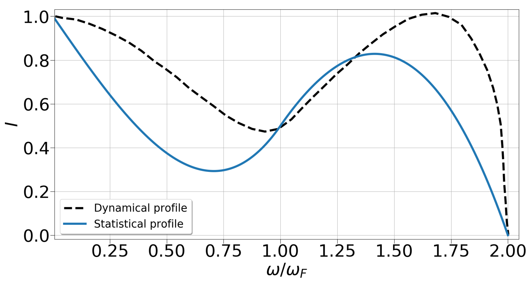
Figure 7 shows a comparison between the statistical and dynamical profiles for the () lines. Both curves are normalized on their maxima, and an appreciable difference between the two types of intensities can be seen. Note that because we have obtained a universal representation, this statement is valid for any plasma parameters within the method’s area of applicability. Thus, it is necessary to account for population kinetics effects for Rydberg states of multi charged ions.
6. Conclusions
In the present review, we have considered Rydberg hydrogen atoms (hydrogen-like ions) in a low-density plasma, demonstrating several methods for spectral line shape calculations. When dealing with the spectra of highly excited atoms or ions, one faces the problem of fast growth of the Rydberg radiative transition array. In the present review, we have obtained a number of solutions to this issue that can help to overcome such difficulties. The semiclassical approach shows good results for an electron in the Coulomb field even when . This circumference was tested for the Balmer spectra in the presence of a constant magnetic filed (Figure 5 and Figure 6). A comparison of the semiclasical approach to experimental data and MD simulation shows good correspondence. We hope that the results presented here can be useful for researchers, as these methods can help to obtain calculations and estimations more quickly and easily. Moreover, even advanced models and MD simulations may not always be in agreement [31]. Thus, within tolerable accuracy limits, the presented approaches could be used in experimental interpretation.
Author Contributions
A.Y.L.: software, writing—original draft preparation, visualization, methodology, investigation. V.S.L.: conceptualization, methodology, project administration, writing—review and editing. All authors have read and agreed to the published version of the manuscript.
Funding
This research received no external funding.
Data Availability Statement
Experimental data for theory validation: Adams, M.L.; Scott, H.A.; Lee, R.W.; Terry, J.L.; Marmar, E.S.; Lipschultz, B.; Pigarov, A.Y.; Freidberg, J.P. Application of Magnetically-Broadened Hydrogenic Line Profiles to Computational Modeling of a Plasma Experiment. J. Quantum Spectrosc. Radiat. Transf. 2001, 71, 117.
Conflicts of Interest
The authors declare no conflict of interest.
References
- Sobel’Man, I.I. Introduction to the Theory of Atomic Spectra: International Series of Monographs in Natural Philosophy; Elsevier: Amsterdam, The Netherlands, 2016; Volume 40. [Google Scholar]
- Landau, L.D.; Lifshitz, E.M. Quantum Mechanics: Non-Relativistic Theory; Elsevier: Amsterdam, The Netherlands, 2013; Volume 3. [Google Scholar]
- Bethe, H.A.; Salpeter, E.E. Quantum Mechanics of Atoms with One and Two Electrons; Pizmatgiz: Moscow, Russia, 1960. [Google Scholar]
- Gorbunov, A.V.; Mukhin, E.E.; Berik, E.B.; Vukolov, K.Y.; Lisitsa, V.S.; Kukushkin, A.S.; Levashova, M.G.; Barnsley, R.; Vayakis, G.; Walsh, M.J. Laser-induced fluorescence for ITER divertor plasma. Fusion Eng. Des. 2017, 123, 695–698. [Google Scholar] [CrossRef]
- Gorbunov, A.V.; Mukhin, E.E.; Berik, E.B.; Melkumov, M.A.; Babinov, N.A.; Kurskiev, G.S.; Tolstyakov, S.Y.; Vukolov, K.Y.; Lisitsa, V.S.; Levashova, M.G.; et al. Laser-induced fluorescence of helium ions in ITER divertor. Fusion Eng. Des. 2019, 146, 2703–2706. [Google Scholar] [CrossRef]
- Mukhin, E.E.; Tolstyakov, S.Y.; Kurskiev, G.S.; Zhiltsov, N.S.; Koval, A.N.; Solovei, V.A.; Gorshkov, A.V.; Asadulin, G.M.; Kornev, A.F.; Makarov, A.V.; et al. Combined Thomson Scattering and Laser-Induced Fluorescence for Studying Divertor and X-point Plasmas in Tokamak with Reactor Technologies. Plasma Phys. Rep. 2022, 48, 866–874. [Google Scholar] [CrossRef]
- Marchuk, O.; Ralchenko, Y.; Janev, R.K.; Biel, W.; Delabie, E.; Urnov, A.M. Concessional excitation and emission of Hnα Stark multiplet in Fusion Plasmas. J. Phys. B At. Mol. Opt. Phys. 2010, 43, 011002. [Google Scholar] [CrossRef]
- Bureyeva, L.A.; Lisitsa, V.S.; Shuvaev, D.A. Statistical and Dynamical Intensities of Atomic Spectral Lines in Plasma. J. Exp. Theor. Phys. 2002, 95, 662–672. [Google Scholar] [CrossRef]
- Demkov, Y.N.; Monozon, B.S.; Ostrovsky, V.N. Energy levels of a hydrogen atom in crossed electric and magnetic fields. Sov. Phys. JETP 1970, 30, 775–776. [Google Scholar]
- Gulyaev, S.A. Profile of the Hn alpha. radio lines in a static ion field. Sov. Astron. AJ (Engl. Transl.) 1976, 20. Available online: http://adsabs.harvard.edu/full/1976SvA....20..573G (accessed on 22 September 2023).
- Gulyaev, S.A. Profile of the Hn beta. radio lines in a static ion field. Sov. Astron. 1978, 22. Available online: http://adsabs.harvard.edu/full/1978SvA....22..572G (accessed on 22 September 2023).
- Fock, V.A. Zur theorie des wasserstoffatoms. Z. Phys. 1935, 98, 145–154. [Google Scholar] [CrossRef]
- Hughes, J.W.B. Stark states and O(4)-symmetry of hydrogenic atoms. Proc. Phys. Soc. 1967, 98, 810–818. [Google Scholar] [CrossRef]
- Novikov, V.G.; Vorob’ev, V.S.; D’yachkov, L.G.; Nikiforov, A.F. Effect of a magnetic field on the radiation emitted by a nonequilibrium hydrogen and deuterium plasma. J. Exp. Theor. Phys. 2001, 92, 441–453. [Google Scholar] [CrossRef]
- Varshalovich, D.A.; Moskalev, A.N.; Khersonskii, V.K. Quantum Theory of Angular Momentum: Irreducible Tensors, Spherical Harmonics, Vector Coupling Coefficients, nj Symbols; World Scientific: Singapore, 2008. [Google Scholar]
- Gordon, W. Zur Berechnung der Matrizen beim Wasserstoffatom. Ann. Phys. 1929, 394, 1031–1056. [Google Scholar] [CrossRef]
- Mosse, C.; Calisti, A.; Stamm, R.; Talin, B.; Bureyeva, L.A.; Lisitsa, V.S. A universal approach to Rydberg spectral line shapes in plasmas. J. Phys. At. Mol. Opt. Phys. 2004, 37, 1343. [Google Scholar] [CrossRef]
- Ferri, S.; Calisti, A.; Mosse, C.; Mouret, L.; Talin, B.; Gigosos, M.A.; Gonzalez, M.A.; Lisitsa, V. Frequency-fluctuation model applied to Stark-Zeeman spectral line shapes in plasmas. Phys. Rev. E 2011, 84, 026407. [Google Scholar] [CrossRef] [PubMed]
- Rosato, J.; Bufferand, H.; Koubiti, M.; Marandet, Y.; Stamm, R. A table of Balmer gamma line shapes for the diagnostic of magnetic fusion plasmas. J. Quant. Spectrosc. Radiat. Transf. 2015, 165, 102–107. [Google Scholar] [CrossRef]
- Rosato, J.; Marandet, Y.; Stamm, R. A new table of Balmer line shapes for the diagnostic of magnetic fusion plasmas. J. Quant. Spectrosc. Radiat. Transf. 2017, 187, 333–337. [Google Scholar] [CrossRef]
- Touati, K.A.; Chenini, K.; Meftah, M.T. Stark-Zeeman Broadening of Spectral Line Shapes in Magnetized Plasmas. Atoms 2020, 8, 91. [Google Scholar] [CrossRef]
- Ferri, S.; Peyrusse, O.; Calisti, A. Stark-Zeeman line-shape model for multi-electron radiators in hot dense plasmas subjected to large magnetic fields. Matter Radiat. Extrem. 2022, 7, 015901. [Google Scholar] [CrossRef]
- Letunov, A.Y.; Lisitsa, V.S. The Coulomb Symmetry and a Universal Representation of Rydberg Spectral Line Shapes in Magnetized Plasmas. Symmetry 2020, 12, 1922. [Google Scholar] [CrossRef]
- Letunov, A.Y.; Lisitsa, V.S. Stark-Zeeman and Blokhincev spectra of Rydberg atoms. J. Theor. Exp. Phys. 2020, 5, 131. [Google Scholar]
- Letunov, A.Y.; Lisitsa, V.S. Spectra of a Rydberg Atom in Crossed Electric and Magnetic Fields. Universe 2020, 6, 157. [Google Scholar] [CrossRef]
- Talin, B.; Calisti, A.; Godbert, L.; Stamm, R.; Lee, R.W.; Klein, L. Frequency-fluctuation model for line shape calculations in plasma spectroscopy. Phys. Rev. A 1995, 51, 1918–1928. [Google Scholar] [CrossRef] [PubMed]
- Bureeva, L.A.; Kadomtsev, M.B.; Levashova, M.G.; Lisitsa, V.S.; Calisti, A.; Talin, B.; Rosmej, F. Equivalence of the method of the kinetic equation and the fluctuating-frequency method in the theory of the broadening of spectral lines. JETP Lett. 2010, 90, 647–650. [Google Scholar] [CrossRef]
- Frisch, U.; Brissaud, A. Theory of Stark broadening-I soluble scalar model as a test. J. Quant. Spectrosc. Radiat. Transf. 1971, 11, 1753–1766. [Google Scholar] [CrossRef]
- Frisch, U.; Brissaud, A. Theory of Stark broadening-II exact line profile with model microfield. J. Quant. Spectrosc. Radiat. Transf. 1971, 11, 1767–1783. [Google Scholar]
- Alexiou, S. Implementation of the Frequency Separation Technique in general line shape codes. High Energy Density Phys. 2013, 9, 375–384. [Google Scholar] [CrossRef]
- Ferri, S.; Calisti, A.; Mosse, C.; Rosato, J.; Talin, B.; Alexiou, S.; Gigosos, M.A.; Gonzalez, M.A.; Gonzalez-Herreo, D.; Lara, N.; et al. Ion Dynamics Effect on Stark-Broadened Line Shapes: A Cross-Comparison of Various Models. Atoms 2014, 2, 299–318. [Google Scholar] [CrossRef]
- Seaton, M.J. Atomic data for opacity calculations. XIII. Line profiles for transitions in hydrogenic ions. J. Phys. B At. Mol. Opt. Phys. 1990, 23, 3255. [Google Scholar] [CrossRef]
- Adams, M.L.; Scott, H.A.; Lee, R.W.; Terry, J.L.; Marmar, E.S.; Lipschultz, B.; Pigarov, A.Y.; Freidberg, J.P. Application of Magnetically-Broadened Hydrogenic Line Profiles to Computational Modeling of a Plasma Experiment. J. Quantum Spectrosc. Radiat. Transf. 2001, 71, 117. [Google Scholar] [CrossRef]
- Kogan, V.I.; Kukushkin, A.B.; Lisitsa, V.S. Kramers Electrodynamics and electron-atomic radiative-collisional processes. Phys. Rep. 1992, 213, 1–116. [Google Scholar] [CrossRef]
- Park, D. Relation between the and spherical eigenfunctions of hydrogen. Zeitschrift fur Physik 1960, 159, 155–1577. [Google Scholar] [CrossRef]
- Herrick, D.R. Sum Rules and Expansion Formula for Stark radiative Transitions in the Hydrogen Atom. Phys. Rev. A 1975, 12, 1949. [Google Scholar] [CrossRef]
- Belyaev, S.T.; Budker, G.I. Multiquant recombination in ionized gases. In Plasma Physics and Problem of Controlled Thermonuclear Reactors; Leontovich, M.A., Ed.; USSR Academy of Science: Moscow, Russia, 1958; Volume 3, 41p. [Google Scholar]
- Landau, L.D.; Lifshitz, E.M. Course of Theoretical Physics: The Classical Theory of Fields; Pergamon: Oxford, UK, 1975; Volume 2. [Google Scholar]
- Kukushkin, A.B.; Lisitsa, V.S. Radiative cascade between Rydberg Atomic States. JETP 1985, 88, 1570–1585. [Google Scholar]
- Flannery, M.R.; Vrinceanu, D. Quantal and Classical Radiative Cascade in Rydberg Plasmas. Phys. Rev. A 2003, 68, 030502. [Google Scholar] [CrossRef]
Figure 1.
The intensity distribution of the spectral line with a fixed value of the electric field F for . The energy shift is measured in units of .
Figure 1.
The intensity distribution of the spectral line with a fixed value of the electric field F for . The energy shift is measured in units of .

Figure 2.
The intensity distribution of the spectral line with a fixed value of the electric field F for . The energy shift is measured in units of .
Figure 2.
The intensity distribution of the spectral line with a fixed value of the electric field F for . The energy shift is measured in units of .

Figure 3.
Normalized intensity profile of the spectral line. The energy shift is measured in units of .
Figure 3.
Normalized intensity profile of the spectral line. The energy shift is measured in units of .

Figure 4.
Normalized intensity profile of the spectral line. The energy shift is measured in units of .
Figure 4.
Normalized intensity profile of the spectral line. The energy shift is measured in units of .

Figure 5.
Normalized intensity profile as a function of the energy shift for the line (transition ), showing a comparison between the universal approach and the experimental data from [33]: T, cm, eV, and the observation direction is perpendicular to the magnetic field.
Figure 5.
Normalized intensity profile as a function of the energy shift for the line (transition ), showing a comparison between the universal approach and the experimental data from [33]: T, cm, eV, and the observation direction is perpendicular to the magnetic field.

Figure 6.
Normalized intensity profile as a function of the energy shift for the line (transition ), showing a comparison between the universal approach and MD simulation calculations from [20]: T, cm, eV, and the observation direction is perpendicular to the magnetic field.
Figure 6.
Normalized intensity profile as a function of the energy shift for the line (transition ), showing a comparison between the universal approach and MD simulation calculations from [20]: T, cm, eV, and the observation direction is perpendicular to the magnetic field.

Figure 7.
Intensity profile showing a comparison between the statistical and dynamical profiles, with the energy shift measured in units of for the spectral line.
Figure 7.
Intensity profile showing a comparison between the statistical and dynamical profiles, with the energy shift measured in units of for the spectral line.

Disclaimer/Publisher’s Note: The statements, opinions and data contained in all publications are solely those of the individual author(s) and contributor(s) and not of MDPI and/or the editor(s). MDPI and/or the editor(s) disclaim responsibility for any injury to people or property resulting from any ideas, methods, instructions or products referred to in the content. |
© 2023 by the authors. Licensee MDPI, Basel, Switzerland. This article is an open access article distributed under the terms and conditions of the Creative Commons Attribution (CC BY) license (https://creativecommons.org/licenses/by/4.0/).
Share and Cite
MDPI and ACS Style
Letunov, A.Y.; Lisitsa, V.S. Review of Rydberg Spectral Line Formation in Plasmas. Atoms 2023, 11, 133. https://doi.org/10.3390/atoms11100133
AMA Style
Letunov AY, Lisitsa VS. Review of Rydberg Spectral Line Formation in Plasmas. Atoms. 2023; 11(10):133. https://doi.org/10.3390/atoms11100133
Chicago/Turabian StyleLetunov, Andrey Yu., and Valery S. Lisitsa. 2023. "Review of Rydberg Spectral Line Formation in Plasmas" Atoms 11, no. 10: 133. https://doi.org/10.3390/atoms11100133
Note that from the first issue of 2016, this journal uses article numbers instead of page numbers. See further details here.