Single Ionization of Helium by Protons of Various Energies in the Parabolic Quasi-Sturmians Approach

Abstract

The parabolic quasi-Sturmian approach, recently introduced for the calculation of ion–atom ionizing collisions, is adapted and applied here to the single ionization of helium induced by an intermediate-energy proton impact. Within the method, the ionization amplitude is represented as the sum of the products of the basis amplitudes associated with the asymptotic behavior of the continuum states of the two noninteracting hydrogenic subsystems $(e^{-},{\mathrm{He}}^{+})$ and $(p^{+},{\mathrm{He}}^{+})$. The $p-e$ interaction is treated as a perturbation in the Lippmann–Schwinger-type (LS) equation for the three-body system $(e^{-},{\mathrm{He}}^{+},p^{+})$. This LS equation is solved numerically using separable expansions for the proton–electron potential. We examine the convergence behavior of the transition amplitude expansion as the number of terms in the representation of the $p-e$ interaction is increased and find that, for some kinematic regimes, the convergence is poor. This difficulty, which is absent for a higher proton energy impact, is solved by varying the momentum of the auxiliary proton plane wave introduced into the basis function. Fully differential cross-sections are calculated and compared with experimental data for 75 keV protons and the results obtained with the 3C model.

1. Introduction

Ionization in the collisions of ions with simple atoms is one of the fundamental processes of atomic dynamics and has been the focus of study for several decades. However, direct measurements of fully differential cross-sections (FDCS), which contain complete collision information, became available only after the development of cold target recoil ion momentum spectroscopy (COLTRIMS) [1,2,3]. For the single ionization of the ground state of helium by high-impact proton energy (1 MeV), FDCS have been recently measured [4] and triggered a number of theoretical calculations [4,5,6,7,8,9,10,11,12]. Despite some unexplained shifts in the angular distributions, overall satisfactory agreement was found. Moreover, those experimental data being on a relative scale, the comparison of absolute theoretical FDCS does not permit us to reach a conclusive statement on the merit of each approach. At a lower impact energy, the absolute FDCS of singly ionizing 75-keV $p-He$ collisions have been measured in various kinematical regimes [13]. For these FDCS, theoretical predictions were obtained based upon the well-known continuum distorted-wave-eikonal initial-state (CDW-EIS) model [14,15], (a) including the projectile and residual target ion interaction (CDW-EIS PI) [16]; (b) the two-Coulomb final wave (2C) + the initial Coulomb projectile wave [17]; (c) the three-Coulomb wave (3C) model [18]; (d) the modified Coulomb–Born approximation (MCB-PI) [19]; (e) the continuum correlated wave model including the interaction between the projectile and the residual target ion (CCW-PT) [20]; (f) including the projectile target core (NN) interaction model convolved with experimental resolution (CDW-EIS NN) [21]. Despite the sophistication of the latest approaches, none of them has managed to reach complete agreement with the experimental data. The most noticeable theory–experiment discrepancies are observed at large values of the transferred momentum. In particular, the proposed theoretical models fail to adequately describe the observed double-peak structure of the FDCS in the perpendicular plane. In the lower-impact energy regime, the electron capture channel may be expected to play an important role and may partially explain such discrepancies. Indeed, the FDCS could be affected, for example, by the well-known Thomas effect [22] that appears when the electron after the second collision with the target nucleus moves in parallel with the same speed as the incident ion. In such a kinematic domain, the particles interact strongly, leading to a resonant increase in the FDCS. Note that the same effect is postulated in a recent work on the Compton disintegration of positronium [23] and is actively discussed in a publication [24] directly related to our study. As far as we know, and although it should be properly taken into account, so far, none of the theoretical approaches modeling the 75 keV measurements [13] have included this channel. Thus, further theoretical developments to describe ion–atom ionizing collisions are required.

Recently [5], some of us proposed the parabolic convoluted quasi-Sturmian (CQS) approach to the FDCS calculation for the ionization process under consideration. The method was successfully tested at high projectile energy, namely with protons at 1 MeV. The results were in good agreement with other theories, and especially with the absolute scale of the WP-CCC approach [25]. In this work, we wish to explore other kinematical situations. We extend the absolute scale comparison with the theoretical predictions of the WP-CCC approach [25] for protons incident at 0.5 and 2 MeV and momentum transfers varying from 0.5 to 1.75 a.u. More importantly, the main aim of this manuscript is to test the applicability and robustness of the CQS approach to a lower incident energy regime (75 keV) for which the absolute measurements [13] offer a serious challenge. In its present version, the CQS approach does not yet include the capture channel, so its application in the lower-energy regime will allow us to compare the cross-sections with those of other theoretical approaches having the same weakness. Clearly, if our CQS approach yields an overall similar picture and if unexplained features (in shape and/or absolute scale) subsist, the inclusion of the capture channel will be identified as the next necessary ingredient to be included in our approach.

Briefly, in the CQS approach [5], one treats the problem in parabolic coordinates with the $\widehat{z}$ axis chosen along the incident proton momentum ${\mathbf{K}}_0$. The ionization amplitude is represented as an expansion in the so-called basis amplitudes associated with the asymptotic behavior of the Green’s functions of the two subsystems $(e^{-},{\mathrm{He}}^{+})$ and $(p^{+},{\mathrm{He}}^{+})$. In both cases, the object of action of the Green’s function operator is the orthogonal complements to the square integrable Sturmian basic functions of the parabolic coordinates. The transition amplitude expansion coefficients are obtained as a solution to the Lippmann–Schwinger (LS) type equation for the final-state three-body system $(e^{-},{\mathrm{He}}^{+},p^{+})$, in which the proton–electron interaction is considered as a perturbation. In order to properly take into account the $p-e$ potential in the intermediate-energy regime under consideration, we introduce into the Sturmian basis functions an auxiliary proton plane wave with a momentum $\mathbf{Q}=\epsilon {\mathbf{K}}_0$, with $\epsilon \le 1$. Contrary to the original implementation proposed in [5], the quantity Q is treated here as a variational parameter that is chosen according to the kinematical values under scrutiny. This modification in the CQS approach is necessary to obtain converged FDCS that can be compared to the 75 keV measurements.

The paper is organized as follows. In Section 2, taking into account the asymptotic behavior of the Green’s function of the Coulomb three-body system $(e^{-},{\mathrm{He}}^{+},p^{+})$ and making the approximation of the frozen-core model for the residual helium ion, we present the main equation of the method. Section 2.1 proposes a representation of its solution in the form of an expansion in terms of convolutions of quasi-Sturmian functions corresponding to noninteracting subsystems $(e^{-},{\mathrm{He}}^{+})$ and $(p^{+},{\mathrm{He}}^{+})$. From this expansion, which presumably converges in the high-energy regime, we deduce the corresponding expansion of the ionization amplitude in terms of the basis amplitudes. In Section 2.2, the matrix representation of the equation for the expansion coefficients of the ionization amplitude is discussed. In particular, the role of the additional pole, which owes its origin to the modification of the exponents of the Sturmian basis functions by introducing the auxiliary proton plane wave $\mathbf{Q}$ in the calculation of the matrix element of the Green’s function, is clarified. We show that by varying Q, we can influence the accuracy of the description of the proton–electron interaction within the framework of this approach. In Section 3, the results of our numerical calculations are presented. First, we examine the convergence issues of the differential ionization cross-sections, particularly with respect to the number of terms in the representation of the proton–electron interaction and the stabilizing role played by the variational parameter Q. Then, we make a comparison with the 75 keV experimental data and theoretical cross-sections obtained by other authors. We also present CQS predictions for FDCS for the cases of 0.5 and 2 MeV protons and compare them with the results of the WP-CCC calculations [25]. Finally, Section 4 provides a summary of this work.

Atomic units (a.u.) in which $\hslash =e=m_e=1$ are used throughout, unless otherwise specified.

2. Theory

We wish to study the ionization process

$$\mathrm{He}\left(1s^2\right)+p^{+}\to e^{-}+p^{+}+{\mathrm{He}}^{+}\left(1s\right)$$

(1)

in which a proton with momentum ${\mathbf{K}}_0$ ionizes the target, ejecting an electron with momentum ${\mathbf{k}}_e$ and energy $k_e^2/2$. The helium nucleus will be considered at rest, and $\mathbf{R}$ will denote the relative coordinate of the proton, which, in the final state, has momentum $\mathbf{K}$. In our model, we take a good ground state representation ${\mathrm{\Phi }}^{\left(0\right)}(\mathbf{r},{\mathbf{r}}^{\prime })$ of the helium target and make the frozen-core approximation for the residual helium ion. In the parabolic CQS approach, the calculation of the amplitude of the ionization process reduces to solving the inhomogeneous equation

$$\left[E-\widehat{H}\right]\left|{\mathrm{\Phi }}^{(+)}\right.〉=\left|{\mathbf{K}}_0,F\right.〉.$$

(2)

The right-hand side of (2) is the product of the plane wave

$$〈\mathbf{R}\left|{\mathbf{K}}_0\right.〉=e^{i{\mathbf{K}}_0·\mathbf{R}}$$

(3)

for the projectile and the matrix element

$$F(\mathbf{R},\mathbf{r})=〈{\psi }_{1s}^{H{e}^{+}}\left|{\widehat{V}}_i\right|{\mathrm{\Phi }}^{\left(0\right)}〉$$

(4)

of the incident channel interaction

$$V_i=\frac{2}{R}-\frac{1}{|\mathbf{R}-\mathbf{r}|}-\frac{1}{|\mathbf{R}-{\mathbf{r}}^{\prime }|}$$

(5)

between the frozen electron wave function ${\psi }_{1s}^{H{e}^{+}}\left({\mathbf{r}}^{\prime }\right)$ and a helium wave function ${\mathrm{\Phi }}^{\left(0\right)}(\mathbf{r},{\mathbf{r}}^{\prime })$. The final three-body channel Hamiltonian

$$\widehat{H}={\widehat{H}}_0+\widehat{U}$$

(6)

is split into a separable part

$${\widehat{H}}_0=-\frac{1}{2m_p}{\nabla }_{\mathbf{R}}^2-\frac{1}{2}{\nabla }_{\mathbf{r}}^2+\frac{1}{R}-\frac{1}{r}$$

(7)

and the proton–electron interaction

$$\widehat{U}=-\frac{1}{\left|\mathbf{R}-\mathbf{r}\right|}$$

(8)

considered as a perturbation.

The ionization amplitude $T_{\mathbf{K},{\mathbf{k}}_e}$ is contained in the leading asymptotic form (for large values of the hyperradius $\rho =\sqrt{m_p{R}^2+r^2}$) of the solution to the driven Equation (2):

$${\mathrm{\Phi }}^{(+)}\left(\mathbf{R},\mathbf{r}\right)\simeq \frac{m_p}{{\left(2\pi \right)}^2}\frac{{\left(2E\right)}^{3/4}{e}^{\frac{i\pi }{4}}}{{\left(2\pi \right)}^{1/2}}\frac{exp\left\{i\left[\sqrt{2E}\rho +W_0(\mathbf{R},\mathbf{r})\right]\right\}}{{\rho }^{5/2}}\frac{1}{\sqrt{2}}{T}_{\mathbf{K},{\mathbf{k}}_e},$$

(9)

where $W_0$ is the Coulomb phase defined by [26]

$$W_0(\mathbf{R},\mathbf{r})=-\frac{\rho }{\sqrt{2E}}\left(\frac{1}{R}-\frac{1}{r}-\frac{1}{\left|\mathbf{R}-\mathbf{r}\right|}\right)ln\left(2\sqrt{2E}\rho \right).$$

(10)

2.1. Parabolic Sturmians

We consider the representation of Equation (2) in the square-integrable Sturmians defined by [27]

$$〈\xi ,\eta ,\varphi |n,m,\varkappa \rangle =\frac{e^{i\varkappa \varphi }}{\sqrt{2\pi }}{\phi }_n^{\left|\varkappa \right|}\left(\xi \right){\phi }_m^{\left|\varkappa \right|}\left(\eta \right),$$

(11)

where

$${\phi }_n^{\lambda }\left(\rho \right)=\sqrt{\frac{2bn!}{(n+\lambda )!}}{\left(2b\rho \right)}^{\lambda /2}{e}^{-b\rho }{L}_n^{\lambda }\left(2b\rho \right),\lambda =\left|\varkappa \right|,$$

(12)

with the basis scale parameter b. The basis vectors are represented by products

$$\left|\mathbf{Q},\mathfrak{N}\right.〉\equiv \left|\mathbf{Q},\mathfrak{n}\right.〉\left|\mathfrak{m}\right.〉$$

(13)

of an auxiliary proton plane wave $\left|\mathbf{Q}\right.〉$ and two Sturmians

$$\left|\mathfrak{n}\right.〉\equiv \left|n_1,n_2,\varkappa \right.〉,\left|\mathfrak{m}\right.〉\equiv \left|m_1,m_2,-\varkappa \right.〉$$

(14)

of the parabolic coordinates ${\xi }_1$, ${\eta }_1$, ${\varphi }_1$ and ${\xi }_2$, ${\eta }_2$, ${\varphi }_2$ corresponding to the proton $\mathbf{R}$ and electron $\mathbf{r}$ position vectors, respectively. Note that the introduced projectile plane wave (it may be compared with the impact parameter model [28], where the proton part of the wave function is approximated in a similar way) is a key ingredient of the approach, as it allows us—albeit partially—to compensate for the oscillating term on the right-hand side of Equation (2). In addition, as will be shown below, we exploit the freedom to choose the value of Q in such a way as to optimize our numerical treatment of the $p-e$ interaction.

Further, we propose to look for the solution ${\mathrm{\Phi }}^{(+)}$ in the form of an expansion

$$\left|{\mathrm{\Phi }}^{(+)}\right.〉=\sum _{\mathfrak{N}}{C}_{\mathfrak{N}}\left|{\mathcal{S}}_{\mathbf{Q},\mathfrak{N}}^{(+)}\right.〉$$

(15)

in terms of CQS functions whose number is determined by some limits M and N to the ranges $\left|\varkappa \right|\le M$ and $n_j,m_j<N$, $j=1,2$. The CQS functions are constructed in such a way as to convey the asymptotic behavior (9) to the solution as completely as possible, namely

$$\left|{\mathcal{S}}_{\mathbf{Q},\mathfrak{N}}^{(+)}\right.〉={\widehat{G}}_0^{(+)}\left(E\right)\left|\mathbf{Q},\tilde{\mathfrak{N}}\right.〉,$$

(16)

where ${\widehat{G}}_0^{(+)}\left(E\right)={\left[E-{\widehat{H}}_0\right]}^{-1}$ and $\left|\mathbf{Q},\tilde{\mathfrak{N}}\right.〉=\left|\mathbf{Q},\tilde{\mathfrak{n}}\right.〉\left|\tilde{\mathfrak{m}}\right.〉$ is the orthogonal complement to the basis vectors $\left|\mathbf{Q},\mathfrak{N}\right.〉$.

Here, the orthogonal complement $\left|\tilde{\mathfrak{l}}\right.〉$ to each Sturmian

$$\left|\mathfrak{l}\right.〉=\left|n,m,\varkappa \right.〉,$$

(17)

is defined by

$$〈\xi ,\eta ,\varphi \left|\tilde{\mathfrak{l}}\right.〉=\frac{4}{\xi +\eta }〈\xi ,\eta ,\varphi \left|n,m,\varkappa \right.〉.$$

(18)

By comparing the CQS (16) asymptotic behavior with (9), it has been found that the amplitude $T_{\mathbf{K},{\mathbf{k}}_e}$ is expressed (up to a phase factor) in terms of so-called basis amplitudes${\mathcal{A}}_{\mathfrak{n}}^{(+)}$ and ${\mathcal{A}}_{\mathfrak{m}}^{(+)}$ [5,29]:

$$T_{\mathbf{K},{\mathbf{k}}_e}=\sqrt{2}2\pi \sum _{\mathfrak{N}}{C}_{\mathfrak{N}}{e}^{i\varkappa ({\varphi }_p-{\varphi }_e)}{\mathcal{A}}_{\mathfrak{n}}^{(+)}({\beta }_p,K,Q;{\theta }_p){\mathcal{A}}_{\mathfrak{m}}^{(+)}({\beta }_e,k_e,0;{\theta }_e),$$

(19)

where ${\beta }_p=\frac{m_p}{K}$ and ${\beta }_e=-\frac{1}{k_e}$ are the Sommerfeld parameters for the two subsystems $(p^{+},{\mathrm{He}}^{+})$ and $(e^{-},{\mathrm{He}}^{+})$. Explicit analytical expressions for these basis amplitudes are provided in [5,29]. The main numerical task consists then of calculating the coefficients $C_{\mathfrak{N}}$.

2.2. Matrix Equation for the Coefficients $C_{\mathfrak{N}}$

Inserting the expansion (15) into (2), and projecting by $\left.〈\mathbf{Q},\mathfrak{N}\right|$, gives the following matrix equation:

$$\sum _{{\mathfrak{N}}^{\prime }}\left[{\delta }_{\mathfrak{N},{\mathfrak{N}}^{\prime }}-\sum _{\mathfrak{M}}\left.〈\mathfrak{N}\right|\widehat{U}\left|\mathfrak{M}\right.〉\left.〈\mathbf{Q},\tilde{\mathfrak{M}}\right|{\widehat{G}}_0^{(+)}\left(E\right)\left|\mathbf{Q},\widetilde{{\mathfrak{N}}^{\prime }}\right.〉\right]C_{{\mathfrak{N}}^{\prime }}=\left.〈\mathfrak{N}\right|{\mathbf{K}}_0-\mathbf{Q},F〉.$$

(20)

In our approach, the $p-e$ potential (8) is treated as a perturbation (in the high-energy regime) and is approximated by a truncated Sturmian basis set (13) expansion

$${\widehat{U}}^{{\mathcal{N}}_0}=\sum _{\mathfrak{N},\mathfrak{M}}\left|\tilde{\mathfrak{N}}\right.〉\left.〈\mathfrak{N}\right|\widehat{U}\left|\mathfrak{M}\right.〉\left.〈\tilde{\mathfrak{M}}\right|,$$

(21)

whose size ${\mathcal{N}}_0=(2M_0+1)N_0^4$ is determined by the limits $M_0$ and $N_0$ to the ranges $\left|\varkappa \right|\le M_0$ and $n_j,m_j<N_0$$(j=1,2)$.

It is intuitively clear that, in the general case, the LS-type equation is inapplicable when taking into account the interaction $\widehat{U}$, which is negligible compared to the energy E. On the other hand, the presence of the proton plane wave $\left|\mathbf{Q}\right.〉$ in the basis function (13) leads to the appearance of the term $-\frac{Q^2}{2m_p}$ in the matrix element of the operator $E-{\widehat{H}}_0$. Roughly speaking, the use of these modified basis functions transforms the energy $E\to E_{eff}=E-\frac{Q^2}{2m_p}$; as a consequence, the values of the matrix elements of the Green’s function operator are increased. Thus, one might expect that there is an optimal value of Q for which the $p-e$ potential can be properly described when using the LS equation.

The matrix elements of the Green’s function are evaluated (numerically) employing the convolution integral representation [30,31]

$$\begin{array}{c}\left.〈\mathbf{Q},\tilde{\mathfrak{N}}\right|{\widehat{G}}_0^{(+)}\left(E\right)\left|\mathbf{Q},\widetilde{{\mathfrak{N}}^{\prime }}\right.〉=\frac{1}{2\pi i}\underset{\mathcal{C}}{\int }d\mathcal{E}\left.〈\tilde{\mathfrak{m}}\right|{\widehat{G}}_C^{(+)}(-1,1;\mathcal{E})\left|\widetilde{{\mathfrak{m}}^{\prime }}\right.〉\\ \times \left.〈\mathbf{Q},\tilde{\mathfrak{n}}\right|{\widehat{G}}_C^{(+)}(1,m_p;E-\mathcal{E})\left|\mathbf{Q},\widetilde{{\mathfrak{n}}^{\prime }}\right.〉,\end{array}$$

(22)

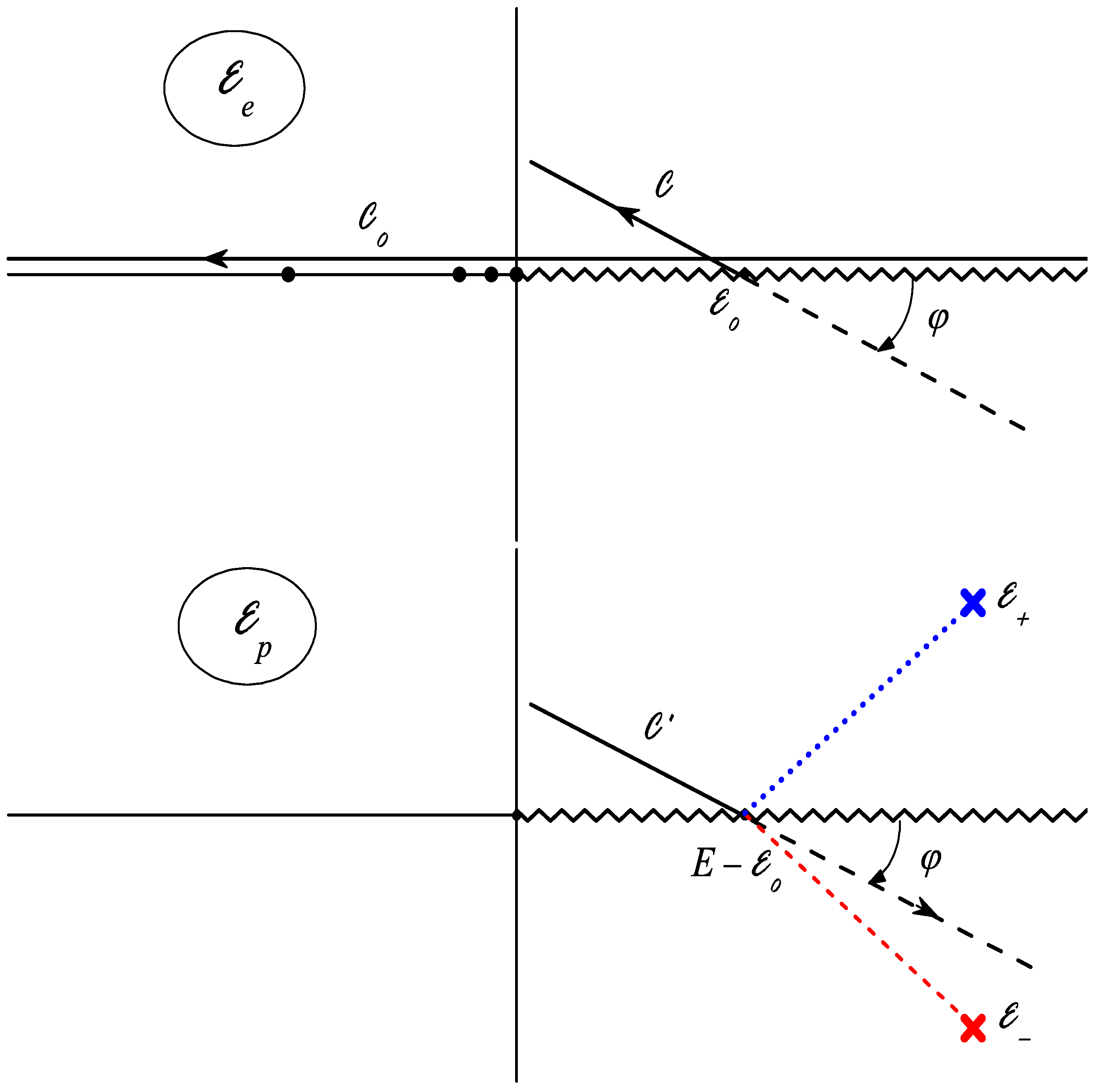
where the path of integration $\mathcal{C}$ is obtained by a rotation of the contour ${\mathcal{C}}_0$ through a negative angle $\phi$ about some point ${\mathcal{E}}_0$ on the positive real axis (see Figure 1). In (22), ${\widehat{G}}_C^{(+)}$ denotes the Green’s function ${\widehat{G}}_C^{(+)}\left(Z,M;\mathcal{E}\right)={\left[\mathcal{E}-{\widehat{H}}_C\right]}^{-1}$ for a Coulomb system with the Hamiltonian

$${\widehat{H}}_C=-\frac{1}{2M}{\nabla }_{\mathbf{X}}^2+\frac{Z}{X},$$

(23)

where $\mathbf{X}$ is the position vector.

The integration contours $\mathcal{C}$ and ${\mathcal{C}}^{\prime }$ in the electron and proton complex energy planes ${\mathcal{E}}_e$ and ${\mathcal{E}}_p$, respectively, are presented in Figure 1. Note that the use of the modified exponents $b-i\frac{Q}{2}$ and $b+i\frac{Q}{2}$ in the proton basis functions ${\phi }_{n_1}^{\lambda }\left({\xi }_1\right)$ and ${\phi }_{n_2}^{\lambda }\left({\eta }_1\right)$, respectively, leads to the appearance of pole singularities in the matrix elements of the proton Green’s function at momenta $P_{\pm }=\pm Q-2ib$. The question arises as to how one should deal with the contribution to the contour integral (22) from the superfluous ‘resonance’ pole at

$${\mathcal{E}}_{-}=\frac{P_{-}^2}{2m_p}=\frac{Q^2-4b^2}{2m_p}-i\frac{2Qb}{m_p},$$

(24)

which lies on the unphysical sheet: $-2\pi \le arg\left({\mathcal{E}}_p\right)<0$. The criterion here can be the condition that the matrix of the Green’s function operator ${\widehat{G}}_0^{(+)}$ must be inverse to the matrix representation of the operator $E-{\widehat{H}}_0$ in the basis set (13). Our numerical calculations show that this condition is satisfied if the residue of this pole is included in the integral. The simplest way to ensure this is to choose a sufficiently small absolute value of the contour rotation angle:

$$\left|\phi \right|<{tan}^{-1}\frac{4Qb}{Q^2-4b^2-2m_p(E-{\mathcal{E}}_0)}$$

(25)

(see Figure 1). We found that in the energy regime considered in the numerical applications, for $Q\le K_0$, the residue of the pole constitutes the lion’s share of the integral (22).

From the above, it follows that the optimal choice for Q, which provides the most accurate account of the proton–electron interaction achievable within our approach, is the admissible value closest to $K_0$. Above such upper bound $Q_0$, the $p-e$ potential can no longer be considered as a perturbation (compared with $E_{eff}$), thus resulting in the very poor convergence of the FDCS as more terms are included in the Sturmian representation (21).

2.3. Numerical Scheme

In summary, the CQS approach to calculating FDCS follows schematically the following steps. First, we set the limits $M_0$ and $N_0$ for the expansion (21) used to represent the perturbation $\widehat{U}$. We also calculate, for a given energy E, the Green’s function matrix elements (22) by adequately choosing Q. With these elements, we solve the matrix Equation (20) and obtain the coefficients $C_{\mathfrak{N}}$. Next, we set the limits M and N for the expansion (15) in CQS and, for given kinematical and geometrical configurations, we sum the basis amplitudes according to (19) and obtain the ionization amplitude $T_{\mathbf{K},{\mathbf{k}}_e}$. Finally, we calculate the FDCS, which, in the laboratory frame, reads

$$\frac{d^5\sigma }{d{E}_{e}d{\mathsf{\Omega }}_{e}d{\mathsf{\Omega }}_p}=k_e\frac{m_p^2}{{\left(2\pi \right)}^5}\frac{K}{K_0}{\left|T_{\mathbf{K},{\mathbf{k}}_e}\right|}^2.$$

(26)

3. Results

All FDCS presented hereafter are on absolute scale.

We start by discussing our CQS results for the FDCS for a proton incident energy of 75 keV and ejected electrons of $5.4$ eV, corresponding to the experimental situation [13]. The experimental FDCS values were measured in absolute scale for electron ejection both into the scattering and into the perpendicular plane at different values of the transverse momentum transfer [13], noted here $\eta$ as in the paper [21].

The CQS calculations have been carried out using a quite accurate ground-state wave function ${\mathrm{\Phi }}^{\left(0\right)}(\mathbf{r},{\mathbf{r}}^{\prime })$ obtained by diagonalizing the helium Hamiltonian matrix representation in the complete square-integrable Laguerre basis set [32]. In this case, the ground-state energy is $E_0=-2.9033$ a.u. For the value of the basis (13) scale parameter $b=1$, the limits $M=3$ and $N=21$ to the ranges $\left|\varkappa \right|\le M$ and $n_j,m_j<N$, $j=1,2$ are sufficient to reach convergence for the 2C-like amplitude, i.e., the ionization amplitude (19) calculated with the $p-e$ potential switched off. In doing this, we put $Q=0$. Then, we switch on the $p-e$ interaction and set the value $Q=K_0$: it was found that for the transverse transferred momenta $\eta =0.13,0.41,0.73$, and $1.38$, the FDCS diverges with the increasing size of the matrix representation (21) of the proton–electron interaction. We thus searched for a more adequate Q value, for each transferred momentum. 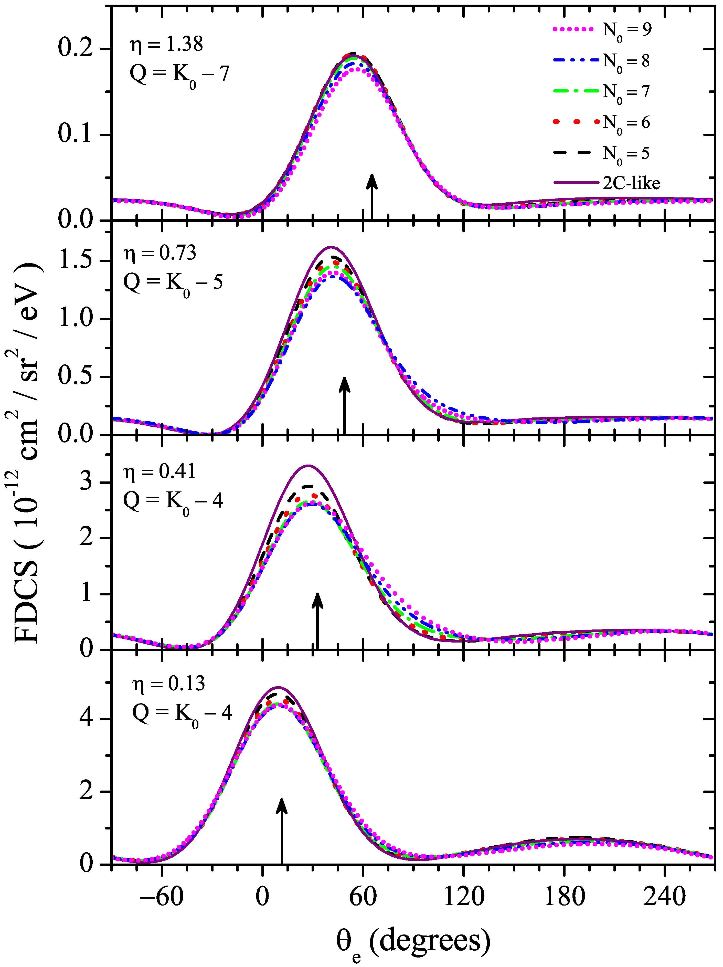Figure 2 presents the FDCS for $M_0=3$ and increasing values of $N_0$ from 5 to 9. It can be seen that the FDCS convergence for $\eta =0.13$ and $\eta =0.41$ is achieved at $K_0-Q=4$, while, for $\eta =0.73$, it is required to increase $K_0-Q$ to 5. Finally, for the largest $\eta =1.38$, a further increase in $K_0-Q$ is necessary. In particular, Figure 2 shows the convergence behavior for $\eta =1.38$ at $K_0-Q=7$.

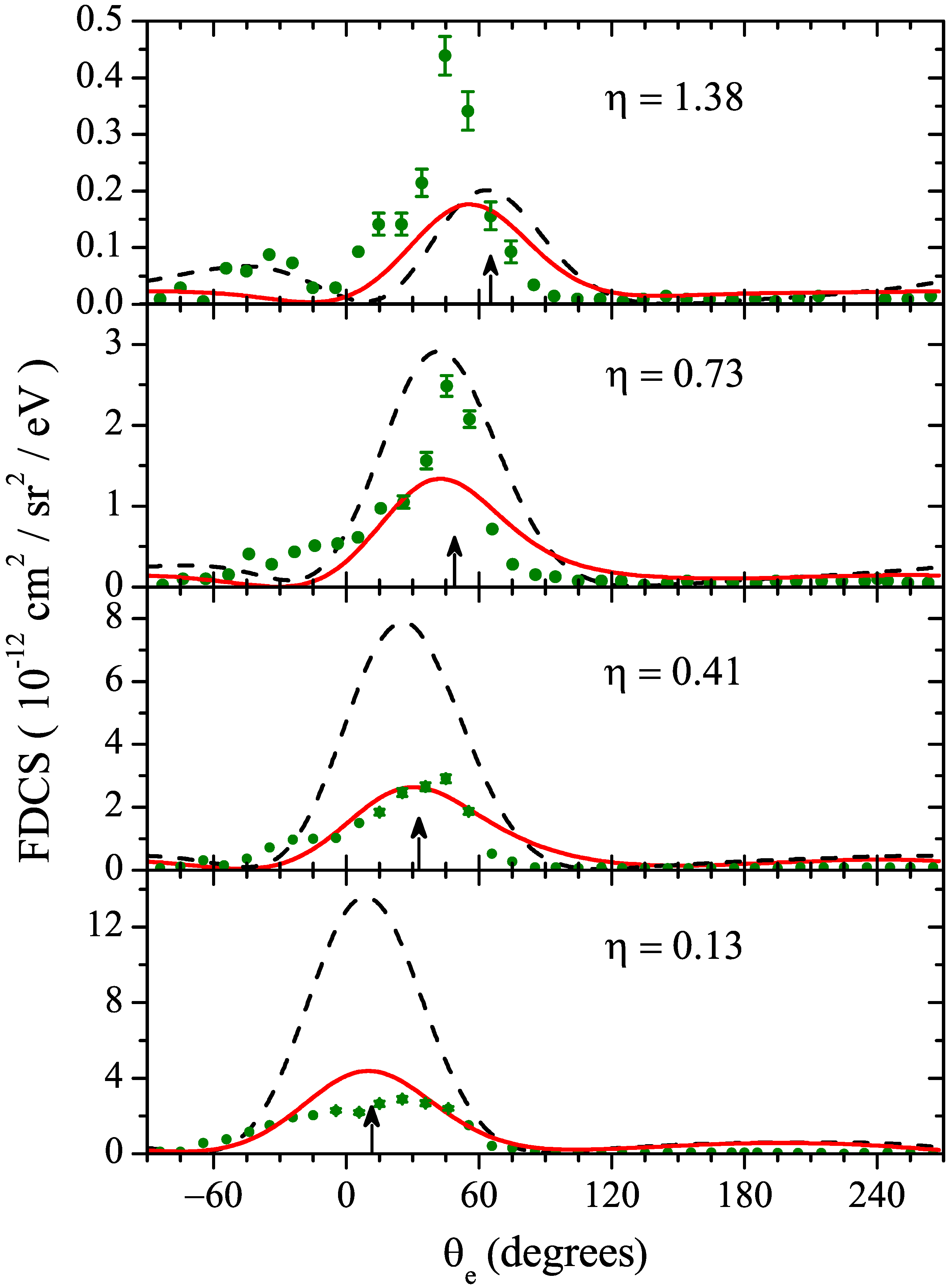
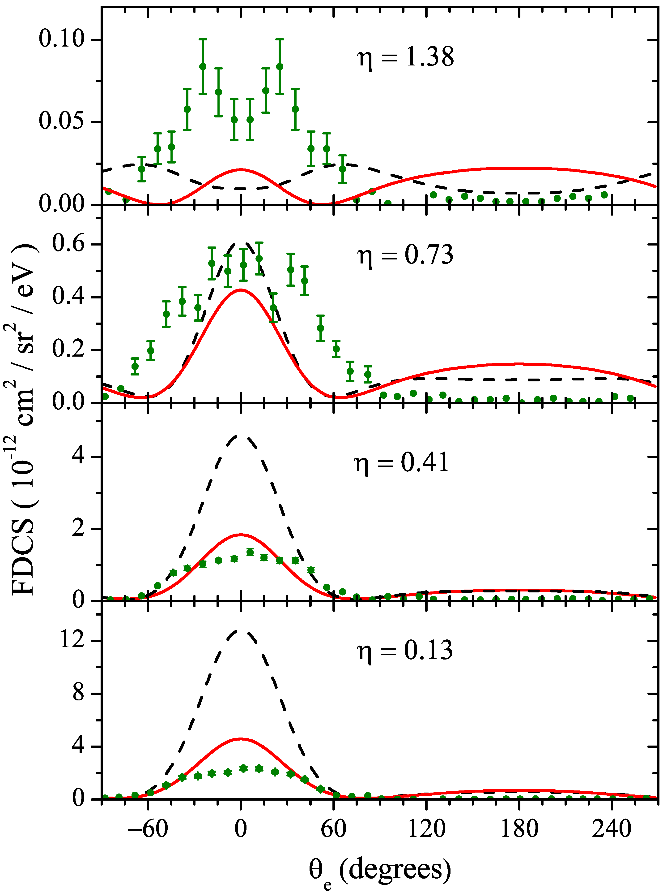
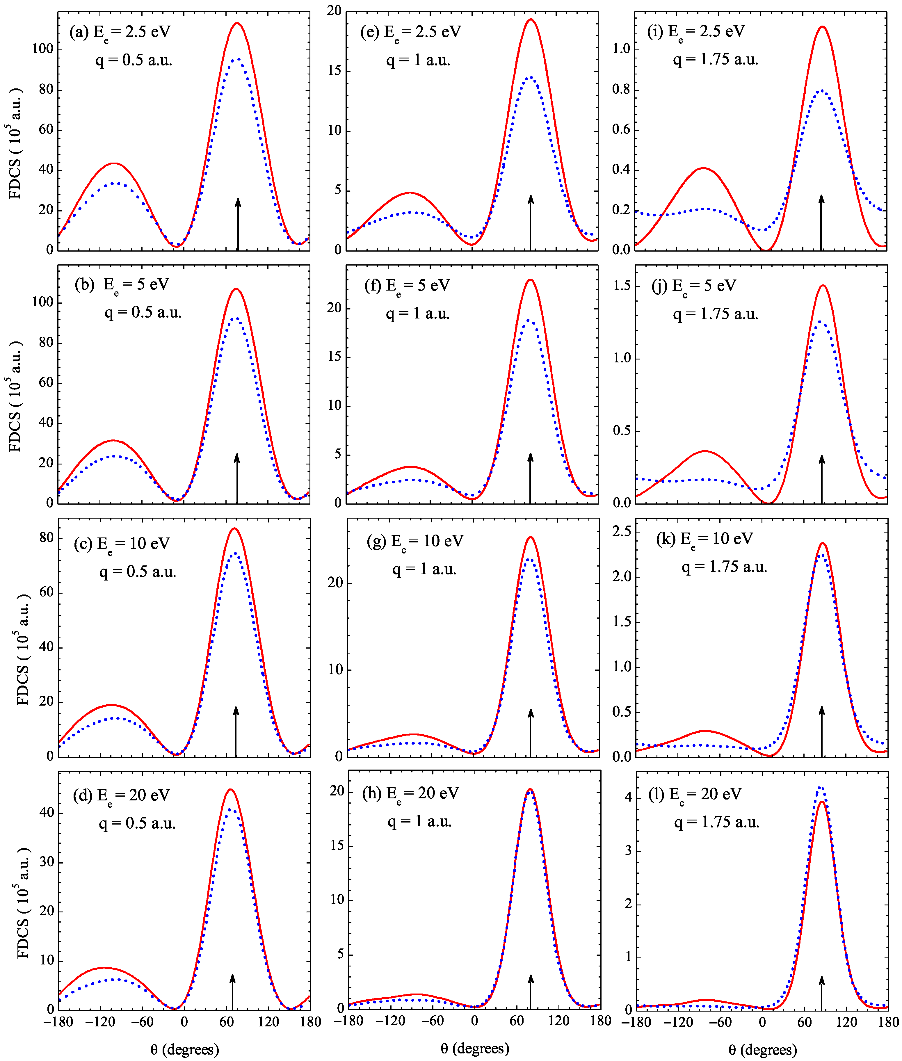
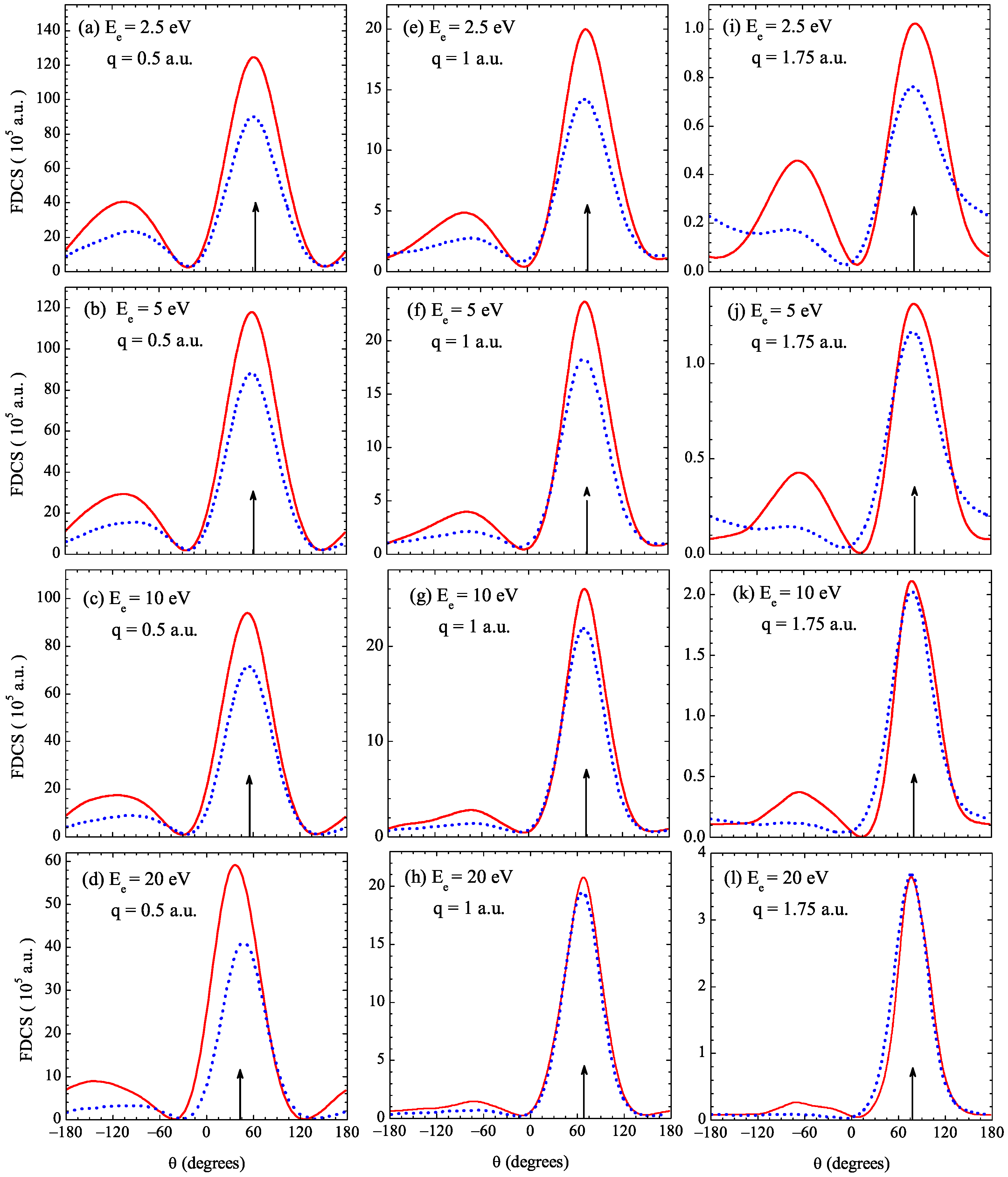
Figure 3 and Figure 4 show our converged CQS results for the ionization FDCS for the collision and perpendicular planes in comparison with the experimental data [13] and the 3C calculations [33]. These 3C results were obtained with a strongly correlated function (CF) [33]; however, we recall that it was found that the 3C predictions for the FDCS depend weakly on the wave function of the helium ground state. The comparison between our CQS and the 3C model calculations is made here in order to focus on the effect of the phase factor (corresponding to the Coulomb proton–electron interaction), which is explicitly present in the 3C wave function.

One can observe that, for all the cases, both the experimental FDCS and the theoretical ones (see also [16,18,19,20,21]) in the scattering plane exhibit a strong peak near the direction of the momentum transfer (indicated in each panel by the arrow). At the same time, the theoretical prediction for the binary peak position is shifted towards smaller angles relative to the experimentally observed value for all momentum transfers, except for $\eta =1.38$.

In the perpendicular plane, the double-peak structure of the measured FDCS at $\eta =1.38$ is reproduced in the 3C model calculations only qualitatively (see also [18]). Similar results were obtained in the MDC-PI [19] and CCW-PT [20] calculations. On the other hand, our CQS calculations (see also Figure 4) do not predict this FDCS feature.

It should be noted that for a proper comparison between the theory and experiments, and between theories, in Figure 2, Figure 3 and Figure 4, all theoretical calculations and the measurements are presented on an absolute scale. This is not the case in some other papers in which scaling factors were purposely used to focus on shapes’ comparison. One should also keep in mind that the calculations do not account for the uncertainties due to the finite energy and angular resolutions of the experiment. Overall, the magnitude of the binary peak in the eight panels is not unreasonable. Another observation is the fact that the recoil to binary peak ratios for the CQS approach are always larger than with the 3C model, except for $\eta =1.38$ and in the scattering plane (see also [18,21]). The absence of experimental points in this angular region, however, does not permit us to favor one approach with respect to the other.

To conclude, we briefly return to the choice of the proton Q value and the convergence problem discussed above. We suspect that the difficulty arises at relatively large proton scattering angles ${\theta }_p$ and not only at large transferred momenta. For example, the value $\eta =1.38$ in the case considered in the experiments corresponds to ${\theta }_p=0.43$ mrad. If we consider the kinematic ionization regimes with impact energies of $0.5$ and 2 MeV (as in [25]), then ${\theta }_p$ does not exceed 0.21 and 0.11 mrad, respectively. In this case, we found convergence of the FDCS already at $Q=K_0$. Thus, within the framework of our approach, it seems that it is the value of the proton scattering angle that is critically important for an adequate description of the proton–electron interaction. Figure 5 and Figure 6 show the CQS and WP-CCC [25] results at, respectively, 2 and 0.5 MeV protons, for a selection of ejected energies and transferred momenta, noted here $\mathbf{q}={\mathbf{K}}_{\mathbf{0}}-\mathbf{K}$. Since this is not always the case when comparing calculations of different theoretical models, it is worth noting that, here, the absolute scale is very similar; the same was observed at 1 MeV [5]. The largest differences are observed at large values of the transferred momentum. It is especially noteworthy that the FDCS obtained by the WP-CCC method does not give the usual sharp two-peak structure, e.g., for $q=1.75$ at $E=2.5$ or 5 or 10 eV. In the CQS results, the main peak is always surrounded by two clear minima (which are practically zero FDCS). Note that from the discussion presented above, in our calculations, the $p-e$ potential is taken into account with the best accuracy achievable within the framework of our approach.

4. Summary

In this paper, the CQS approach is applied to the calculation of the FDCS for proton–helium ionization at an impact energy of 75 keV. In contrast to the case of high projectile energy, in this intermediate regime, we are faced with the problem of adequately describing the $p-e$ interaction when using the LS-type equation for the three-body system $(e^{-},{\mathrm{He}}^{+},p^{+})$. Specifically, in the general case, the transition amplitudes show a lack of convergence as the number of terms in the Sturmian representation of the proton–electron potential is increased. In order to improve the convergence rate for small $\eta$ and achieve convergence in the case of large $\eta$ values, we use the auxiliary proton plane wave momentum Q as a variable parameter, the optimal choice of which allows us to solve this problem.

From the performed calculations, we deduced that the critically important parameter affecting the rate of convergence of the cross-section with an increase in the size of the $p-e$ interaction matrix representation is not the transferred momentum $\eta$ itself, but the value of the proton scattering angle ${\theta }_p$. To test this hypothesis, we also calculated the FDCS for the incident proton energies of 0.5 and 2 MeV explored in [25]. For these values, in spite of rather significant transferred momenta, there was no need to resort to varying the parameter Q in the CQS approach, since the FDCS convergence is already achieved at $Q=K_0$. As for the 1 MeV case analyzed in [5], we compared our CQS cross-sections for 0.5 and 2 MeV with the WP-CCC predictions; globally, the shapes and the magnitudes are quite similar, but, for specific kinematic regimes, some discrepancies are observed, particularly in the recoil region.

For the 75 keV kinematics, considerable discrepancies in the shape of the angular distributions are observed between the experimental data and our calculated FDCS, both in the scattering and in the perpendicular plane. A similar overall picture is found when comparing the measured FDCS with other theoretical predictions. It follows from our calculations that the proper treatment of the Coulomb proton–electron potential plays a key role at intermediate energies of the incident proton. In particular, at such energies, the discussed ionization channel competes with the electron capture channel. This indicates that some loosely accounted features of the dynamics in the $(e^{-},p^{+})$ subsystem, such as contributions to the FDCS from virtual proton–electron bound states, might be responsible for the observed discrepancies between our CQS calculations and experiment. Thus, the goal of our further research will be to develop our approach by improving the description of proton–electron dynamics. The first step in this direction will be the explicit inclusion of the proton–electron states, similar to what the authors of Ref. [34] intend to do. Specifically, we are going to redesign the present formulation so that the role of ‘perturbation’ is played by the interaction between the projectile and the residual ion, rather than the projectile–electron potential (8), while the spectra of subsystems $(e^{-},{\mathrm{He}}^{+})$ and $(e^{-},p^{+})$ are taken into account completely in terms of the corresponding CQS functions.