Article

Quadrupole Effects in the Photoionisation of Sodium 3s in the Vicinity of the Dipole Cooper Minimum

1
School of Physical Sciences, Indian Institute of Technology Mandi, Kamand 175075, India
2
Department of Physics, Indian Institute of Technology Patna, Bihta 801103, India
3
Department of Physics and CAMOST, Indian Institute of Technology Tirupati, Tirupati 517619, India
4
Department of Physics, Dayananda Sagar University, Bengaluru 560078, India
5
Department of Physics and Astronomy, Georgia State University, Atlanta, GA 30303, USA
*
Author to whom correspondence should be addressed.
Atoms 2023, 11(10), 125; https://doi.org/10.3390/atoms11100125
Submission received: 8 August 2023 / Revised: 19 September 2023 / Accepted: 21 September 2023 / Published: 28 September 2023

Abstract

:
A procedure to obtain relativistic expressions for photoionisation angular distribution parameters using the helicity formulation is discussed for open-shell atoms. Electric dipole and quadrupole transition matrix elements were considered in the present work, to study the photoionisation dynamics of the 3s electron of the sodium atom in the vicinity of the dipole Cooper minimum. We studied dipole–quadrupole interference effects on the photoelectron angular distribution in the region of the dipole Cooper minimum. Interference with quadrupole transitions was found to alter the photoelectron angular distribution, even at rather low photon energies. The initial ground and final ionised state discrete wavefunctions of the atom were obtained in the present work using GRASP, and we employed RATIP with discrete wavefunctions, to construct continuum wavefunctions and to calculate transition amplitudes, total cross-sections and angular distribution asymmetry parameters.

1. Introduction

In the majority of studies of light–matter interaction, the dipole approximation is used. It is generally applicable when electromagnetic radiation has a wavelength much larger than the size of the atomic or molecular system. In the dipole approximation ( e i k r 1 ), where k is the wavenumber of the incident photon, one neglects the spatial variation of the electromagnetic field over the target system. Non-dipole effects are important at short wavelengths, and have prompted several atomic and molecular studies [1,2,3,4,5] in condensed matter physics [6] and astrophysics [7]. The emergence of intense laser light sources, such as the free-electron laser (FEL) [8,9,10], have further revealed the importance of non-dipole interactions in explaining photoelectron spectra, especially in relation to non-linear absorption and time-resolved studies.
The importance of non-dipole effects has been highlighted by several authors, in both experimental and theoretical works [3,11,12,13,14,15,16,17,18,19,20,21,22,23,24,25]. These studies have revealed that dipole–quadrupole (E1–E2) interference affects the angular distribution of photoelectrons, due to first-order corrections to the dipole approximation, even at rather low energies. Numerous studies are available for closed-shell systems, but those on open-shell systems, especially using relativistic methodologies, are few [26,27]. To the best of our knowledge, relativistic calculations, including interchannel coupling, are not available for open-shell atoms.
Higher multipole corrections to total subshell cross-sections become important for photon energies more than a few keV above the ionisation threshold. However, a number of situations exist in photoionisation processes that demand going beyond the dipole approximation, even at energies as low as a few eV [28,29,30,31,32,33,34,35,36,37,38,39,40]. Instances where the quadrupole transition amplitudes are comparatively larger than the electric dipole transition amplitudes occur in regions of the dipole Cooper minimum, dipole/quadrupole autoionisation resonances, etc. The present work was motivated by an earlier work by Pradhan et al. [37], which showed the importance of non-dipole effects in the case of Mg 3s photoionisation at rather low photon energies, due to the presence of the Cooper minimum in the 3s dipole ionisation channel. We explored a similar situation for the case of a typical open-shell atom, viz., sodium, by studying the photoionisation of its valence shell in the photon energy range 5.14 eV to 7 eV. The 3s dipole photoionisation goes through the Cooper minimum in this region. The required non-dipole angular distribution parameters were obtained, following an earlier work by Huang [41,42], which used helicity eigenstates to study the dynamics. This formulation is applicable to both open- and closed-shell systems [41,42]. On the other hand, the methodology described in Derevianko et al. [43] is applicable only to closed-shell systems. Below, we briefly present an overview of the procedure to include non-dipole effects in the photoelectron angular distribution asymmetry parameters for s-subshell photoionisation. The required transition amplitudes were determined in the present work by using a combination of two computational algorithms, namely, the General-Purpose Relativistic Atomic Structure Program (GRASP) [44,45,46] and the Relativistic calculations of Atomic Transition, Ionisation and recombination Properties (RATIP) [47]. The combination of GRASP and RATIP has already been successfully applied in a number of cases studying atomic structure and dynamics [48,49,50,51]. In the present work, a single configuration initial state of photoionisation was considered, but a multi-configuration initial state could also be considered.
In Section 2, details of the helicity formalism [41,42], along with the important steps involved in the derivation of the required photoelectron angular distribution parameters by a linearly polarised light, are discussed. The results of our calculations are discussed in Section 3. The important findings of this work are summarised in Section 4.

2. Theory

This section is divided into three sub-sections. In Section 2.1, the salient features of the helicity formulation of photoelectron angular distribution from references [41,42] are summarised. References [41,42] provide the form of β , and we explicitly discuss the various steps involved in arriving at the equations in Section 2.2. The general expression for the differential cross-section is available in the work of Huang [41,42], but not the expressions for non-dipole angular distribution asymmetry parameters. Explicit expressions for angular distribution asymmetry parameters inclusive of the quadrupole terms are developed and presented in Section 2.3 for the first time, to the best of our knowledge. Also provided is a brief discussion of second-order non-dipole photoelectron angular distribution parameters.

2.1. Photoionisation Dynamics Based on Helicity Formalism

Conventionally, the photoionisation transition matrix element is constructed using angular-momentum eigenstates. However, in the helicity formalism, angular-momentum eigenstates are transformed to helicity eigenstates. This approach was first adopted by Lee [52] for the non-relativistic formulation of photoionisation processes in the electric dipole approximation. This was extended to the relativistic regime by Huang [41,42]. In this work, the reduced matrix element D α ( E j ) , for photoionisation in the Coulomb gauge for an electric 2 j - pole transition ( E j ), is given by
D ( E j ) ( κ α ) = i α e i δ κ α α J i = 1 N α · A ( E j ) ( r i ) J 0 .
Here, δ κ α is the Coulomb phase shift of the photoelectron in the particular channel κ α = ( α j α ) , and A ( E j ) is the normalised electric multipole vector potential, while j and J 0 are, respectively, the total angular momenta of the photon and the initial states of the atom. J represents the total angular momentum of the photoelectron plus the ionised atom system. A similar expression of the reduced matrix element can be obtained for the magnetic 2 j -pole transitions, and is defined by D ( M j ) ( κ α ) .
The expression for the angle-dependent differential cross-section, including all multipole transitions in helicity formalism [41,42], is
d σ ( θ , ϕ ) d Ω = σ 4 π F ( θ , ϕ ) ,
where σ is the total photoionisation cross-section and F ( θ , ϕ ) is an angular distribution function given by
F ( θ , ϕ ) = 1 + 1 B 0 d 00 + ( S x cos ( 2 ϕ ) + S y sin ( 2 ϕ ) ) 2 B 1 d 20 ,
where S x , S y and S z are the Stokes parameters of the incident light, d m n denotes the ‘d’ functions of the rotation matrices and θ and ϕ are the polar and azimuthal angles of the emitted photoelectron (of total angular momentum j α ), with respect to the incident photon direction k ^ , as shown in Figure 1a. In the above expression,
B 0 = j J j α j J j α ( 1 ) J 0 J α + 1 / 2 σ ¯ j J j α j J j α 2 J J j α j α J α J J j j J 0 j α j α 1 / 2 1 / 2 0 j j 1 1 0 × π + π k + ( 1 ) k / 2 ( E E + M M ) + π k ( 1 ) ( k + 1 ) / 2 ( E M M E ) cos ( δ α δ α ) + π π k ( 1 ) ( k + 1 ) / 2 ( E E + M M ) π k + ( 1 ) k / 2 ( E M M E ) sin ( δ α δ α )
and,
B 1 = j J j α j J j α ( 1 ) J 0 J α + 1 / 2 σ ¯ j J j α j J j α 2 J J j α j α J α J J j j J 0 j α j α 1 / 2 1 / 2 0 j j 1 1 2 × π + π k + ( 1 ) k / 2 ( E E M M ) π k ( 1 ) ( k + 1 ) / 2 ( E M + M E ) cos ( δ α δ α ) + π π k ( 1 ) ( k + 1 ) / 2 ( E E M M ) + π k + ( 1 ) k / 2 ( E M + M E ) sin ( δ α δ α ) .
The summation j J j α j J j α takes into account the interference between various transition matrix elements, and δ α is the phase of the reduced matrix element, D ( E j ) ( κ α ) . In the above expressions, J α is the total angular momentum of the ionised state of the atom. B 0 l and B 1 l correspond to various multipole terms arising from electric–electric, electric–magnetic and magnetic–magnetic interactions. Here, σ ¯ = j J κ α | D ( E j ) ( κ α ) | 2 + | D ( M j ) ( κ α ) | 2 , σ = 8 π 4 c / ω [ J 0 ] 2 σ ¯ , and E | D ( E j ) ( κ α ) | . Similarly, M | D ( M j ) ( κ α ) | . Note that [ j ] = 2 j + 1 . The effects of magnetic interactions are very weak compared to electric interactions, and hence are neglected in the present work. Furthermore, π ± and π k ± in Equations (4) and (5) are defined as follows:
π + π = 1 ( 0 ) is even 0 ( 1 ) is odd
π k + π k = 1 ( 0 ) k is even 0 ( 1 ) k is odd ,
where is the summation index in Equation (3), k = j j and ‘ + / ’ correspond to even/odd.
A photon with linear momentum vector k is not in an eigenstate of the angular momentum j. However, being a massless particle, it has a definite value of helicity, which is the component of the angular momentum in the direction of the photon momentum. Now, for the electromagnetic waves (being transverse) the total angular momentum can take the values j = 1 , 2 , 3 , [53]. The infinite series in Equation (3) can be truncated, depending on the level of approximation considered, by making use of the Wigner 3j selection rules. The truncation procedure at the level of dipole, quadrupole and octupole approximations are discussed below.

2.2. Dipole Approximation

In the electric dipole approximation, j = j = 1 . The values in the Wigner 3j symbols, j j 1 1 0 and j j 1 1 2 , of Equations (4) and (5) range from | j j | to j + j , giving = 0 , 1 and 2. The summations begin from = 1 for the second term and = 2 for the third term of Equation (3). Hence, under the dipole approximation, only takes values 1 and 2. In this particular case, the variable k in Equations (4) and (5) is an even number ( π k + ), because k is given by j j , which is zero. Since is odd and k is even, the only term that needs to be considered in Equation (4) is the one that involves the electric and magnetic interactions. However, in the dipole approximation, magnetic interactions do not appear and, hence, B 01 = 0 . Therefore, only = 2 contributes in the dipole approximation giving rise to B 02 and B 12 . The Wigner 3j symbols of Equations (4) and (5), j j 1 1 0 and j j 1 1 2 give 1 / 30 and 1 / 5 , respectively, for j = j = 1 and = 2 . Using B 01 and B 02 along with Equation (3), Equation (2) reduces to
d σ d Ω = σ 4 π 1 + B 02 d 00 2 + S x cos 2 ϕ + S y sin 2 ϕ B 12 d 20 2 .
The right-hand side of Equations (4) and (5) for = 2 can be written in terms of a single parameter, β 1 (a dipole asymmetry parameter), as follows: B 02 = β 1 / 2 and B 12 = 3 / 2 β 1 , where β 1 is
β 1 = 30 ( 1 ) J 0 J α + 1 / 2 σ ¯ j J j α j J j α J j α J j α J J 2 j α j α J α J J 2 1 1 J 0 j α j α 2 1 / 2 1 / 2 0 E E cos ( δ α δ α ) .
The term S 1 cos 2 ϕ + S 2 sin 2 ϕ in (8) is expressed as p cos 2 α cos ( 2 ( ϕ γ ) ) . Here, the parameters p, α and γ can be understood as follows. Consider a coordinate system XYZ, such that the Z axis is in the direction of the photon flux, as shown in Figure 2. The X axis is chosen conveniently to determine the photon polarisation. The parameter γ specifies the azimuthal orientation of the polarisation. When the photon polarisation vector coincides with the X axis, γ = 0 . The angle between the electric field vectors at their successive crests is α . In case of linearly polarised light, α = 0 . The probability p ( 0 p 1 ) of complete polarisation is referred to as the degree of polarisation of the photon. The degree of polarisation p = 1 for pure linearly polarised incident photons. In Equation (8), d 00 2 = P 2 ( cos θ ) and d 20 2 = 3 2 2 sin 2 θ . Using these above relations, Equation (8) can be further reduced to
d σ d Ω = σ 4 π 1 1 2 β 1 P 2 ( cos θ ) 3 2 p cos 2 α cos ( 2 ( ϕ γ ) ) sin 2 θ .
It is often convenient to express the above equation in an alternate co-ordinate system, as shown in Figure 1b, where θ ¯ corresponds to the angle between the photoelectron momentum and the polarisation direction, and where ϕ ¯ corresponds to the angle between the propagation vector and the projection of momentum vector in the X-Y plane. Under this new co-ordinate system, Equation (10) reduces to
d σ d Ω = σ 4 π 1 + β 1 P 2 ( cos θ ¯ )
for linearly polarised light, where α = 0 and p = 1 .

2.3. Beyond Dipole Approximation

Including quadrupole interactions, j and j can take values 1 and 2. Consequently, takes values 1 3 . The variable k = j j can be 1 and 1, which implies that k is odd for the dipole and quadrupole interference terms. The even and the odd k can contribute only via electric–magnetic interactions. Since they are neglected in the present work, B 02 = 0 . Therefore, the only terms that contribute to the quadrupole approximation are B 01 , B 03 and B 13 , which are rewritten in terms of Γ 1 and Γ 3 as follows:
Γ 1 = 3 3 2 ( 1 ) J 0 J α + 1 / 2 σ ¯ j J j α j J j α J j α J j α J J 1 j α j α J α J J 1 j j J 0 j α j α 1 1 / 2 1 / 2 0 ( 1 ) ( k + 1 ) / 2 E E sin ( δ α δ α ) ,
Γ 3 = 21 ( 1 ) J 0 J α + 1 / 2 σ ¯ j J j α j J j α J j α J j α J J 3 j α j α J α J J 3 j j J 0 j α j α 3 1 / 2 1 / 2 0 ( 1 ) ( k + 1 ) / 2 E E sin ( δ α δ α ) ,
where Γ 1 = B 01 and Γ 3 = B 03 = 3 / 10 B 13 . Using these, the differential cross-section for the photoionisation, given in Equation (3), with the inclusion for first-order quadrupole terms, can be expressed as
d σ d Ω = σ 4 π 1 + Γ 1 P 1 ( cos θ ) 1 2 β 2 P 2 ( cos θ ) + Γ 1 P 3 ( cos θ ) + 3 4 β 2 5 2 Γ 3 cos θ p cos 2 α cos ( 2 ( ϕ γ ) ) sin 2 θ .
Note that the dipole asymmetry parameter β 1 is now written as β 2 under the quadrupole approximation. The expression for β 2 differs from β 1 only in the σ ¯ term in the denominator of Equation (9). With the inclusion of non-dipole interactions, σ ¯ = J κ α | D ( E 1 ) ( κ α ) | 2 + | D ( E 2 ) ( κ α ) | 2 . In general, the dipole amplitude dominates the quadrupole amplitude. It can be, therefore, easily seen that this additional term in σ ¯ only plays a major role when the dipole amplitude goes through a minima. We again transform the representation of d σ / d Ω from ( θ , ϕ ) ( θ ¯ , ϕ ¯ ) :
d σ d Ω = σ 4 π 1 + β 2 P 2 ( cos θ ¯ ) + Γ 1 + Γ 3 5 Γ 3 cos 2 θ ¯ sin θ ¯ cos ϕ ¯ .
The usual experimental scheme to measure these non-dipole parameters is to set θ ¯ = 54.7 ° and ϕ ¯ = 0 ° . The differential cross-section at these angles is
d σ d Ω = σ 4 π 1 + 2 3 Γ 1 + Γ 3 5 3 Γ 3 .
It is convenient to write δ = Γ 1 + Γ 3 and γ = 5 Γ 3 , so that
d σ d Ω = σ 4 π 1 + 2 27 3 δ + γ ,
where the combined quantity 3 δ + γ can be extracted from a measurement. Equation (15) is re-written in terms of δ and γ :
d σ d Ω = σ 4 π 1 + β 2 P 2 ( cos θ ¯ ) + δ + γ cos 2 θ ¯ sin θ ¯ cos ϕ ¯ .
This is in agreement with Derevianko et al.’s [43] expression for d σ / d Ω while considering only the electric dipole and lowest order quadrupole interactions, which works for the closed-shell system. The above expression can also be written as d σ / d Ω = σ 1 + A ( θ ¯ , ϕ ¯ ) / 4 π , where A ( θ ¯ , ϕ ¯ ) provides the angular distribution associated with the photoelectron ejection.
The above procedure can be further extended to higher-order terms. If we include the second-order correction, the differential cross-section can be expressed as follows:
d σ d Ω = σ 4 π 1 + B 01 E 1 , E 2 d 00 1 + B 02 E 1 , E 1 + B 02 E 1 , E 3 + B 02 E 2 , E 2 × d 00 2 + B 03 E 1 , E 2 d 00 3 + B 04 E 1 , E 3 + B 04 E 2 , E 2 d 00 4 + S x cos 2 ϕ S y sin 2 ϕ × B 12 E 1 , E 1 + B 12 E 1 , E 3 + B 12 E 2 , E 2 d 20 2 + B 13 E 1 , E 2 d 20 3 + B 14 E 1 , E 3 + B 14 E 2 , E 2 d 20 4 .
In Section 3, we present the results obtained using the above-mentioned procedures; in particular, the quadrupole effects in the photoionisation of Na 3s. The calculations considered are those of single configurations. The photon–atom interaction resulting in the emission of an electron with a residual ion, for dipole transitions, is expressed as ω ( j = 1 ) + N a 1 s 2 2 s 2 2 p 6 3 s 1 2 S J 0 = 1 / 2 N a + 1 s 2 2 s 2 2 p 6 1 S J α = 0 + ϵ p j α = 1 / 2 , ϵ p j α = 3 / 2 . Similarly, for the quadrupole transitions, ω ( j = 2 ) + N a 1 s 2 2 s 2 2 p 6 3 s 1 2 S J 0 = 1 / 2 N a + 1 s 2 2 s 2 2 p 6 1 S J α = 0 + ϵ d j α = 3 / 2 , ϵ d j α = 5 / 2 . The transition amplitudes required for these calculations were calculated using a combination of two software packages, GRASP and RATIP.

3. Results and Discussion
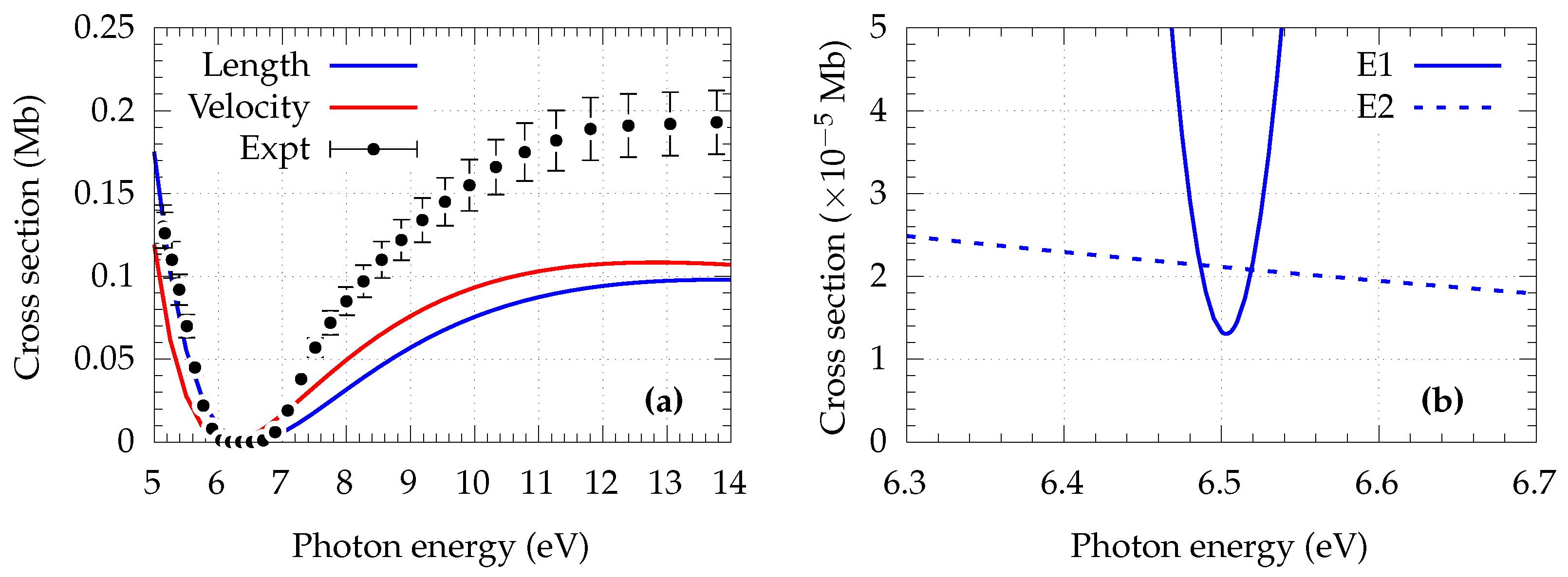
3.1. Cross-Section

Figure 3a shows the Na 3s cross-section, calculated at the dipole approximation level in the length and velocity gauges, which is in reasonable agreement with the experimental data in the energy range 5.14 to 7 eV, even at the single configuration level of calculation. This region is particularly interesting, because of the presence of the dipole Cooper minimum here. Above 7 eV, there is a disagreement with the experimental data, and the agreement between length and velocity deteriorates. This may be due to the absence of initial state correlation in the present calculation. However, the present work was aimed at the Cooper minimum region below 7 eV, where there is a reasonable agreement between theory and experiment. Figure 3b shows the dipole and quadrupole cross-sections in the length gauge. This shows that the quadrupole cross-section was larger than the dipole cross-section at the dipole minimum over a small range of photon energies ∼0.03 eV. It is to be noted that although the cross-section is going through the Cooper minimum, the cross-section was not zero, even at the single configuration level. This was because of the relativistic interactions resulting from the s ϵ p 1 / 2 and s ϵ p 3 / 2 transitions, which underwent their respective minima at slightly different energies. For simplicity, these final states are denoted ϵ p + and ϵ p , respectively [54].
Direct experimental measurements provide information only about the sum of the dipole (E1) and quadrupole (E2) cross-sections. Information about the relative magnitudes of E1 and E2 individually is not available from experiment. However, this information can be extracted from angular distribution studies. Previous studies have shown that, at low energies, the effect of non-dipole interactions is more significant on the angular distribution parameters than the cross-section [28,29,30,31,32,33,34,35,36,37,38,39,40]. To understand the effect of quadrupole transitions on photoelectron angular distributions, we examine the asymmetry parameters.

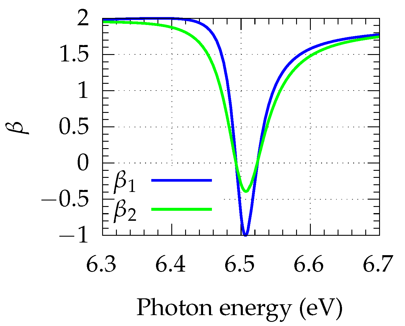
3.2. Dipole Parameter, β

The equation for the asymmetry parameter for a half-filled n s subshell at the dipole approximation level can be deduced from Equation (9), by making appropriate substitutions of angular momentum values. We denote the transition matrix elements by D α D ( E 1 ) ( κ α ) for dipole, and Q α D ( E 2 ) ( κ α ) for quadrupole terms. This turns out to be
β 1 = | D ϵ p + | 2 2 2 | D ϵ p | | D ϵ p + | cos ( δ p δ p + ) | D ϵ p | 2 + | D ϵ p + | 2 .
Subscript 1 is used in β , to indicate that this determines the angular distribution parameter in the dipole approximation. In the absence of relativistic effects, β 1 = 2 . This can be seen by re-writing Equation (19) in terms of radial matrix elements. The reduced matrix elements and the radial matrix elements are related as follows: D ϵ p = 2 / 3 R ϵ p = 2 / 3 | R ϵ p | e i ( δ ϵ p + π ) and D ϵ p + = + 4 / 3 R ϵ p + = 4 / 3 | R ϵ p + | e i δ ϵ p + . Here, δ ϵ p ± represents the phase of the radial matrix elements, R ϵ p ± . The term π is included, along with δ ϵ p , to account for the negative sign accompanying the radial matrix element R ϵ p . Note that δ ϵ p δ ϵ p + π and δ ϵ p + δ ϵ p + . In the non-relativistic limit, | R ϵ p | = | R ϵ p + | and δ ϵ p = δ ϵ p + , resulting in cos ( δ ϵ p δ ϵ p + ) = cos ( π ) , which reduces Equation (19) to its non-relativistic value, 2.
Figure 4 shows rapid variation of the asymmetry parameter β 1 in the region of the Cooper minimum. Under the dipole approximation, the value of β 1 is ≈2 over most of the energy range, except in the region of the Cooper minimum, where it undergoes a dip and takes a value close to 1 , as expected [56]. However, when the quadrupole interactions are taken into account, the above formula is modified, as discussed in Section 2. The expression for the asymmetry parameter is modified, with an additional term in the denominator, which is denoted as β 2 . It is easy to show that these two parameters are related via the following equation:
β 2 = β 1 × κ α | D κ α | 2 | D κ α | 2 + | Q κ α | 2 .
From the above equation, it can be deduced that the factor multiplied by β 1 can take values unity or less. Thus, the deviation in the region of the Cooper minimum becomes shallower when non-dipole interactions are present, as shown in Figure 4. In the absence of non-dipole interactions, β 1 goes all the way to 1 in the Cooper minimum region. This amounts to a stronger yield in the direction perpendicular to the polarisation of the photon. The inclusion of non-dipole terms causes the dip in the Cooper minimum region to be close to zero ( β 2 0 ), which corresponds to the photoelectron angular distribution being roughly isotropic in comparison to β 1 . The present work, therefore, shows the importance of non-dipole interactions in determining the photoelectron yield in different directions, even at low energies.

3.3. Quadrupole Parameters Γ 1 and Γ 3

By making suitable substitutions in Equations (12) and (13), we arrive at the expressions for Γ 1 and Γ 3 for the photoionisation of a half-filled n s subshell:
Γ 1 = 2 σ ¯ 3 2 | Q 3 / 2 | | D 1 / 2 | sin ( δ 3 / 2 δ 1 / 2 ) 3 10 | Q 3 / 2 | | D 3 / 2 | sin ( δ 3 / 2 δ 3 / 2 ) + 9 5 2 | Q 5 / 2 | | D 3 / 2 | sin ( δ 5 / 2 δ 3 / 2 ) ,
Γ 3 = 2 σ ¯ | Q 5 / 2 | | D 1 / 2 | sin ( δ 5 / 2 δ 1 / 2 ) 3 3 5 | Q 3 / 2 | | D 3 / 2 | sin ( δ 3 / 2 δ 3 / 2 ) + 4 5 2 | Q 5 / 2 | | D 3 / 2 | sin ( δ 5 / 2 δ 3 / 2 ) .
These parameters, Γ 1 and Γ 3 , are plotted in Figure 5. They are nearly zero in the region away from the Cooper minimum, and they show rapid variation near the Cooper minimum. Recall from Section 2 that Γ 1 + Γ 3 = δ (also shown in Figure 5) and γ = 5 Γ 3 . The features of Γ 1 and Γ 3 can be better understood in their non-relativistic limits. The relations between the quadrupole reduced matrix elements and radial matrix elements are Q ϵ d = 4 / 5 R ϵ d = 4 / 5 | R ϵ d | e i δ d and Q ϵ d + = 6 / 5 R ϵ d + = 6 / 5 | R ϵ d + | e i ( δ d + + π ) . The corresponding relations for the dipole matrix elements are discussed in Section 3.2. Using these relations, Equations (21) and (22) can be reduced to their non-relativistic limits:
Γ 1 = 6 6 6 | D | 2 + 5 | Q 2 | | Q | | D | sin ( δ Q δ D ) ,
Γ 3 = 6 6 6 | D | 2 + 5 | Q 2 | | Q | | D | sin ( δ Q δ D ) .
It is easily seen that the non-relativistic δ vanishes, since Γ 1 = Γ 3 for the n s subshell. In the regions away from the CM, Q D . Hence, it becomes evident from the above expressions that Γ 1 and Γ 3 are directly proportional to Q / D , resulting in their values being nearly zero. In the region where the dipole amplitude, D, undergoes the Cooper minimum, the ratio becomes larger. At the dipole CM, there is a phase jump of π , leading to the sign flip of Γ 1 and Γ 3 . All these features are preserved, even in the relativistic Γ 1 and Γ 3 , except for the fact that δ = Γ 1 + Γ 3 has non-zero values in the region of the CM. This can be attributed to the fact that relativistic dipole channels are undergoing the CM at slightly different energies, which deviates the δ from its non-relativistic value.
As discussed in Section 2.3, one of the experimentally relevant parameters is γ = 5 Γ 3 . The significant values of γ and its strong dependence on photon energy show that the photoelectron angular distribution (PAD) is very sensitive to photon energy in the region of the Cooper minimum. To illustrate this, the shape of the photoelectron angular distribution, 1 + A ( θ ¯ , ϕ ¯ ) , is plotted for a few selected energies, and is shown in Figure 6 in 2D (the xz plane) and 3D. In order to bring out the role of the quadrupole effects, the PAD obtained with and without the inclusion of the quadrupole interactions (denoted as 1 + A ( θ ¯ , ϕ ¯ ) E 1 E 2 and 1 + A ( θ ¯ , ϕ ¯ ) E 1 , respectively) are shown. In the absence of relativistic and/or non-dipole effects, the angular distribution is essentially cos 2 θ ¯ . Here, the preferential direction (or direction of maximum yield) of photoelectron ejection is along the polarisation direction ϵ ^ . This is seen at a photon energy of 5.25 eV. Both 1 + A ( θ ¯ , ϕ ¯ ) E 1 and 1 + A ( θ ¯ , ϕ ¯ ) E 1 E 2 show a dipolar distribution, since this is well below the Cooper minimum, where non-dipole interactions do not play any significant role in the dynamics. The values of β 1 β 2 = 1.93 (close to the non-relativistic value 2), Γ 1 = 0.05 and Γ 3 = 0.05 are smaller, because Q is significantly less than D, as seen in Figure 3.
Figure 6b,d show the PAD at photon energies 6.48 eV and 6.54 eV, where both Γ 1 and Γ 3 take extremum values, due to the presence of the Cooper minimum. At 6.48 eV, Γ 1 = 0.97 , Γ 3 = 1.07 , β 1 = 1.14 and β 2 = 0.65 , whereas at 6.54 eV the values are Γ 1 = 0.92 , Γ 3 = 0.82 , β 1 = 0.80 and β 2 = 0.58 . As a result, 1 + A ( θ ¯ , ϕ ¯ ) E 1 E 2 at these energies significantly differs from 1 + A ( θ ¯ , ϕ ¯ ) E 1 . The direction of the maximum photoelectron yield moves away from ϵ ^ at these energies for 1 + A ( θ ¯ , ϕ ¯ ) E 1 E 2 , i.e., with the inclusion of quadrupole effects.
Also shown, in Figure 6c, is the PAD at a photon energy of 6.51 eV, where Γ 1 + Γ 3 is at its minimum. The shape of PAD 1 + A ( θ ¯ , ϕ ¯ ) E 1 E 2 significantly deviates from PAD 1 + A ( θ ¯ , ϕ ¯ ) E 1 . For 1 + A ( θ ¯ , ϕ ¯ ) E 1 , the yield is zero along the ϵ ^ ; however, it is non-zero when the quadrupole effects are considered, although the preferential direction remains the same in both cases. It is important to note that the above determination of the PAD employs only the first-order non-dipole parameters in the present work, which is valid, as long as D Q . However, as seen from Figure 3b, the quadrupole cross-section (and, thus, the matrix element Q) is larger than the dipole matrix element D between 6.48 eV and 6.52 eV. In this region, the second-order E2–E2 interference terms will not only be important but dominant. Thus, Figure 6b–d should only be considered representative of the effects of first-order non-dipole corrections, but do not represent physical reality, since the E2–E2 terms are not included in the description of the PAD. For example, the small petal-like structures in Figure 6b,d are artefacts of the first-order approximations. They will no longer appear if the second corrections are included. The methodology developed here can be extended, to incorporate the E2–E2 interference effect, and work in this direction is in progress.

4. Conclusions

Following the earlier work on photoionisation dynamics based on helicity formalism [41,42], explicit relativistic formulae for angular distribution parameters, including the dipole and quadrupole interference effects, were derived for the n s subshells for cases of open-shell atomic systems. Using the formulae obtained, the photoionisation dynamics of Na 3s were studied in the region of the dipole Cooper minimum, which demonstrated the importance of quadrupole transitions in determining the angular distribution at low photon energies (≈7 eV). Although the calculations were done at the level of single-particle approximation, they could be extended, to include multi-electron effects, by replacing the matrix elements obtained by single configuration calculation with that of multi-configuration calculation, using GRASP and RATIP. The methodology developed here could also be extended to higher-order multi-pole interactions and to other subshells. We hope the current work will stimulate photoionisation dynamics studies of open-shell systems, studies that would highlight both relativistic and multi-electron effects.

Author Contributions

Conceptualization, N.M.H. and H.R.V.; Methodology, N.M.H. and H.R.V.; Software, N.M.H. and J.J.; Formal analysis, N.M.H., J.J., H.R.V., P.C.D. and S.T.M.; Investigation, N.M.H., J.J., H.R.V., P.C.D. and S.T.M.; Writing—original draft, N.M.H.; Writing—review & editing, J.J., H.R.V., P.C.D. and S.T.M.; Supervision, H.R.V. All authors have read and agreed to the published version of the manuscript.

Funding

Two of the authors, Nishita M. Hosea and Hari R. Varma, extend their gratitude to the Science and Engineering Research Board, Department of Science and Technology, Government of India, for funding this work, Grant Number CRG/2022/002309. The work of Steven T. Manson was supported by the US Department of Energy, Office of Basic Sciences, Division of Chemical Science, Geosciences and Biosciences, under Grant No. DE-FG02-03ER15428.

Data Availability Statement

The data generated and/or analysed during the current study are available from the corresponding author on a reasonable request.

Conflicts of Interest

The authors declare no conflict of interest.

References

  1. Hemmers, O.; Guillemin, R.; Lindle, D.W. Nondipole effects in soft X-ray photoemission. Radiat. Phys. Chem. 2004, 70, 123–147. [Google Scholar] [CrossRef]
  2. Guillemin, R.; Hemmers, O.; Lindle, D.W.; Manson, S.T. Experimental investigation of nondipole effects in photoemission at the advanced light source. Radiat. Phys. Chem. 2006, 75, 2258–2274. [Google Scholar] [CrossRef]
  3. Hemmers, O.; Guillemin, R.; Rolles, D.; Wolska, A.; Lindle, D.W.; Kanter, E.P.; Krässig, B.; Southworth, S.H.; Wehlitz, R.; Zimmermann, B.; et al. Low-energy nondipole effects in molecular nitrogen valence-shell photoionization. Phys. Rev. Lett. 2006, 97, 103006. [Google Scholar] [CrossRef] [PubMed]
  4. Cherepkov, N.A.; Semenov, S.K. Non-dipole effects in spin polarization of photoelectrons from Xe 4p and 5p shells. J. Phys. B At. Mol. Opt. Phys. 2001, 34, L211. [Google Scholar] [CrossRef]
  5. Khalil, T.; Schmidtke, B.; Drescher, M.; Müller, N.; Heinzmann, U. Experimental verification of quadrupole-dipole interference in spin-resolved photoionization. Phys. Rev. Lett. 2002, 89, 053001. [Google Scholar] [CrossRef]
  6. Jensen, S.V.B.; Madsen, L.B. Propagation time and nondipole contributions to intraband high-order harmonic generation. Phys. Rev. A 2022, 105, L021101. [Google Scholar] [CrossRef]
  7. Tyndall, N.B.; Ramsbottom, C.A.; Ballance, C.P.; Hibbert, A. Photoionization of Co+ and electron-impact excitation of Co2+ using the Dirac R-matrix method. Mon. Not. R. Astron. Soc. 2016, 462, 3350–3360. [Google Scholar] [CrossRef]
  8. Emma, P.; Akre, R.; Arthur, J.; Bionta, R.; Bostedt, C.; Bozek, J.; Brachmann, A.; Bucksbaum, P.; Coffee, R.; Decker, F.J.; et al. First lasing and operation of an ångstrom-wavelength free-electron laser. Nat. Photonics 2010, 4, 641–647. [Google Scholar] [CrossRef]
  9. McNeil, B.W.; Thompson, N.R. X-ray free-electron lasers. Nat. Photonics 2010, 4, 814–821. [Google Scholar] [CrossRef]
  10. Ishikawa, T.; Aoyagi, H.; Asaka, T.; Asano, Y.; Azumi, N.; Bizen, T.; Ego, H.; Fukami, K.; Fukui, T.; Furukawa, Y.; et al. A compact X-ray free-electron laser emitting in the sub-ångström region. Nat. Photonics 2012, 6, 540–544. [Google Scholar] [CrossRef]
  11. Lindle, D.W.; Hemmers, O. Breakdown of the dipole approximation in soft-X-ray photoemission. J. Electron Spectrosc. Relat. Phenom. 1999, 100, 297–311. [Google Scholar] [CrossRef]
  12. Bechler, A.; Pratt, R. Higher retardation and multipole corrections to the dipole angular distribution of 1s photoelectrons at low energies. Phys. Rev. A 1989, 39, 1774. [Google Scholar] [CrossRef]
  13. Bechler, A.; Pratt, R. Higher multipole and retardation corrections to the dipole angular distributions of L-shell photoelectrons ejected by polarized photons. Phys. Rev. A 1990, 42, 6400. [Google Scholar] [CrossRef] [PubMed]
  14. Cooper, J.W. Multipole corrections to the angular distribution of photoelectrons at low energies. Phys. Rev. A 1990, 42, 6942. [Google Scholar] [CrossRef] [PubMed]
  15. Cooper, J.W. Erratum: Multipole corrections to the angular distribution of photoelectrons at low energies [Phys. Rev. A 42, 6942 (1990)]. Phys. Rev. A 1992, 45, 3362. [Google Scholar] [CrossRef] [PubMed]
  16. Cooper, J. Photoelectron-angular-distribution parameters for rare-gas subshells. Phys. Rev. A 1993, 47, 1841. [Google Scholar] [CrossRef]
  17. Krässig, B.; Jung, M.; Gemmell, D.; Kanter, E.; LeBrun, T.; Southworth, S.; Young, L. Nondipolar asymmetries of photoelectron angular distributions. Phys. Rev. Lett. 1995, 75, 4736. [Google Scholar] [CrossRef]
  18. Hemmers, O.; Fisher, G.; Glans, P.; Hansen, D.; Wang, H.; Whitfield, S.; Wehlitz, R.; Levin, J.; Sellin, I.; Perera, R.C.; et al. Beyond the dipole approximation: Angular-distribution effects in valence photoemission. J. Phys. B At. Mol. Opt. Phys. 1997, 30, L727. [Google Scholar] [CrossRef]
  19. Dolmatov, V.K.; Manson, S.T. Enhanced nondipole effects in low energy photoionization. Phys. Rev. Lett. 1999, 83, 939. [Google Scholar] [CrossRef]
  20. Amusia, M.Y.; Baltenkov, A.; Felfli, Z.; Msezane, A. Large nondipole correlation effects near atomic photoionization thresholds. Phys. Rev. A 1999, 59, R2544. [Google Scholar] [CrossRef]
  21. Derevianko, A.; Hemmers, O.; Oblad, S.; Glans, P.; Wang, H.; Whitfield, S.B.; Wehlitz, R.; Sellin, I.A.; Johnson, W.; Lindle, D.W. Electric-octupole and pure-electric-quadrupole effects in soft-X-ray photoemission. Phys. Rev. Lett. 2000, 84, 2116. [Google Scholar] [CrossRef] [PubMed]
  22. Amusia, M.Y.; Baltenkov, A.; Chernysheva, L.; Felfli, Z.; Msezane, A. Nondipole parameters in angular distributions of electrons in photoionization of noble-gas atoms. Phys. Rev. A 2001, 63, 052506. [Google Scholar] [CrossRef]
  23. Johnson, W.R.; Cheng, K. Strong nondipole effects in low-energy photoionization of the 5 s and 5 p subshells of xenon. Phys. Rev. A 2001, 63, 022504. [Google Scholar] [CrossRef]
  24. Cherepkov, N.A.; Semenov, S.K. On quadrupole resonances in atomic photoionization. J. Phys. B At. Mol. Opt. Phys. 2001, 34, L495. [Google Scholar] [CrossRef]
  25. Hemmers, O.; Guillemin, R.; Kanter, E.; Krässig, B.; Lindle, D.W.; Southworth, S.; Wehlitz, R.; Baker, J.; Hudson, A.; Lotrakul, M.; et al. Dramatic Nondipole Effects in Low-Energy Photoionization: Experimental and Theoretical Study of Xe 5 s. Phys. Rev. Lett. 2003, 91, 053002. [Google Scholar] [CrossRef]
  26. Trzhaskovskaya, M.; Nikulin, V.; Nefedov, V.; Yarzhemsky, V. Non-dipole second order parameters of the photoelectron angular distribution for elements Z = 1–100 in the photoelectron energy range 1–10 keV. At. Data Nucl. Data Tables 2006, 92, 245–304. [Google Scholar] [CrossRef]
  27. Trzhaskovskaya, M.; Nefedov, V.; Yarzhemsky, V. Photoelectron angular distribution parameters for elements Z = 1 to Z = 54 in the photoelectron energy range 100–5000 eV. At. Data Nucl. Data Tables 2001, 77, 97–159. [Google Scholar] [CrossRef]
  28. Leuchs, G.; Smith, S.; Dixit, S.; Lambropoulos, P. Observation of interference between quadrupole and dipole transitions in low-energy (2-eV) photoionization from a sodium Rydberg state. Phys. Rev. Lett. 1986, 56, 708. [Google Scholar] [CrossRef]
  29. Martin, N.; Thompson, D.; Bauman, R.; Caldwell, C.; Krause, M.; Frigo, S.; Wilson, M. Electric-dipole–quadrupole interference of overlapping autoionizing levels in photoelectron energy spectra. Phys. Rev. Lett. 1998, 81, 1199. [Google Scholar] [CrossRef]
  30. Grum-Grzhimailo, A. Non-dipole effects in magnetic dichroism in atomic photoionization. J. Phys. B At. Mol. Opt. Phys. 2001, 34, L359. [Google Scholar] [CrossRef]
  31. Krässig, B.; Kanter, E.; Southworth, S.; Guillemin, R.; Hemmers, O.; Lindle, D.W.; Wehlitz, R.; Martin, N. Photoexcitation of a dipole-forbidden resonance in helium. Phys. Rev. Lett. 2002, 88, 203002. [Google Scholar] [CrossRef] [PubMed]
  32. Kanter, E.; Krässig, B.; Southworth, S.; Guillemin, R.; Hemmers, O.; Lindle, D.W.; Wehlitz, R.; Amusia, M.Y.; Chernysheva, L.; Martin, N. E 1-E 2 interference in the vuv photoionization of He. Phys. Rev. A 2003, 68, 012714. [Google Scholar] [CrossRef]
  33. Lépine, F.; Zamith, S.; de Snaijer, A.; Bordas, C.; Vrakking, M. Observation of large quadrupolar effects in a slow photoelectron imaging experiment. Phys. Rev. Lett. 2004, 93, 233003. [Google Scholar] [CrossRef] [PubMed]
  34. Dolmatov, V.; Bailey, D.; Manson, S. Gigantic enhancement of atomic nondipole effects: The 3 s→ 3 d resonance in Ca. Phys. Rev. A 2005, 72, 022718. [Google Scholar] [CrossRef]
  35. Deshmukh, P.; Banerjee, T.; Varma, H.R.; Hemmers, O.; Guillemin, R.; Rolles, D.; Wolska, A.; Yu, S.; Lindle, D.W.; Johnson, W.; et al. Theoretical and experimental demonstrations of the existence of quadrupole Cooper minima. J. Phys. B At. Mol. Opt. Phys. 2008, 41, 021002. [Google Scholar] [CrossRef]
  36. Argenti, L.; Moccia, R. Nondipole effects in helium photoionization. J. Phys. B At. Mol. Opt. Phys. 2010, 43, 235006. [Google Scholar] [CrossRef]
  37. Pradhan, G.; Jose, J.; Deshmukh, P.; LaJohn, L.; Pratt, R.; Manson, S. Cooper minima: A window on nondipole photoionization at low energy. J. Phys. B At. Mol. Opt. Phys. 2011, 44, 201001. [Google Scholar] [CrossRef]
  38. Gryzlova, E.; Grum-Grzhimailo, A.; Strakhova, S.; Meyer, M. Non-dipole effects in the angular distribution of photoelectrons in sequential two-photon double ionization: Argon and neon. J. Phys. B At. Mol. Opt. Phys. 2013, 46, 164014. [Google Scholar] [CrossRef]
  39. Gryzlova, E.; Grum-Grzhimailo, A.; Kuzmina, E.; Strakhova, S. Sequential two-photon double ionization of noble gases by circularly polarized XUV radiation. J. Phys. B At. Mol. Opt. Phys. 2014, 47, 195601. [Google Scholar] [CrossRef]
  40. Ilchen, M.; Hartmann, G.; Gryzlova, E.; Achner, A.; Allaria, E.; Beckmann, A.; Braune, M.; Buck, J.; Callegari, C.; Coffee, R.; et al. Symmetry breakdown of electron emission in extreme ultraviolet photoionization of argon. Nat. Commun. 2018, 9, 4659. [Google Scholar] [CrossRef]
  41. Huang, K.N. Theory of angular distribution and spin polarization of photoelectrons. Phys. Rev. A 1980, 22, 223. [Google Scholar] [CrossRef]
  42. Huang, K.N. Addendum to “Theory of angular distribution and spin polarization of photoelectrons”. Phys. Rev. A 1982, 26, 3676. [Google Scholar] [CrossRef]
  43. Derevianko, A.; Johnson, W.; Cheng, K. Non-dipole effects in photoelectron angular distributions for rare gas atoms. At. Data Nucl. Data Tables 1999, 73, 153–211. [Google Scholar] [CrossRef]
  44. Dyall, K.; Grant, I.; Johnson, C.; Parpia, F.; Plummer, E. GRASP: A general-purpose relativistic atomic structure program. Comput. Phys. Commun. 1989, 55, 425–456. [Google Scholar] [CrossRef]
  45. Parpia, F.A.; Fischer, C.F.; Grant, I.P. GRASP92: A package for large-scale relativistic atomic structure calculations. Comput. Phys. Commun. 1996, 94, 249–271. [Google Scholar] [CrossRef]
  46. Jönsson, P.; Gaigalas, G.; Bieroń, J.; Fischer, C.F.; Grant, I. New version: Grasp2K relativistic atomic structure package. Comput. Phys. Commun. 2013, 184, 2197–2203. [Google Scholar] [CrossRef]
  47. Fritzsche, S. The Ratip program for relativistic calculations of atomic transition, ionization and recombination properties. Comput. Phys. Commun. 2012, 183, 1525–1559. [Google Scholar] [CrossRef]
  48. Hütten, K.; Mittermair, M.; Stock, S.O.; Beerwerth, R.; Shirvanyan, V.; Riemensberger, J.; Duensing, A.; Heider, R.; Wagner, M.S.; Guggenmos, A.; et al. Ultrafast quantum control of ionization dynamics in krypton. Nat. Commun. 2018, 9, 719. [Google Scholar] [CrossRef] [PubMed]
  49. Perry-Sassmannshausen, A.; Buhr, T.; Borovik, A., Jr.; Martins, M.; Reinwardt, S.; Ricz, S.; Stock, S.; Trinter, F.; Müller, A.; Fritzsche, S.; et al. Multiple photodetachment of carbon anions via single and double core-hole creation. Phys. Rev. Lett. 2020, 124, 083203. [Google Scholar] [CrossRef]
  50. Schippers, S.; Beerwerth, R.; Bari, S.; Buhr, T.; Holste, K.; Kilcoyne, A.D.; Perry-Sassmannshausen, A.; Phaneuf, R.A.; Reinwardt, S.; Savin, D.W.; et al. Near L-edge single and multiple photoionization of doubly charged iron ions. Astrophys. J. 2021, 908, 52. [Google Scholar] [CrossRef]
  51. Hosea, N.M.; Jose, J.; Varma, H.R. Near-threshold Cooper minimum in the photoionisation of the 2p subshell of sodium atom and its impact on the angular distribution parameter. J. Phys. B At. Mol. Opt. Phys. 2022, 55, 135001. [Google Scholar] [CrossRef]
  52. Lee, C. Spin polarization and angular distribution of photoelectrons in the Jacob-Wick helicity formalism. Application to autoionization resonances. Phys. Rev. A 1974, 10, 1598. [Google Scholar] [CrossRef]
  53. Landau, L.; Lifshitz, E. A Shorter Course of Theoretical Physics. Vol. 2: Quantum Mechanics; Pergamon: Oxford, UK, 1974. [Google Scholar]
  54. Seaton, M.J. A comparison of theory and experiment for photo-ionization cross-sections II. Sodium and the alkali metals. Proc. R. Soc. Lond. Ser. A. Math. Phys. Sci. 1951, 208, 418–430. [Google Scholar]
  55. Hudson, R.D.; Carter, V.L. Atomic absorption cross sections of lithium and sodium between 600 and 1000 Å. J. Opt. Soc. Am. 1967, 57, 651–654. [Google Scholar] [CrossRef]
  56. Manson, S.T.; Starace, A.F. Photoelectron angular distributions: Energy dependence for s subshells. Rev. Mod. Phys. 1982, 54, 389. [Google Scholar] [CrossRef]
Figure 1. Transforming from the co-ordinate system ( θ , ϕ ) to the co-ordinate system ( θ ¯ , ϕ ¯ ) . The co-ordinate ( θ ¯ , ϕ ¯ ) is obtained by rotating the co-ordinate ( θ , ϕ ) by 180 about the z-axis and 90 about the y-axis.
Atoms 11 00125 g001
Figure 2. Types of polarisation.
Atoms 11 00125 g002
Figure 3. (a) Total cross-section of sodium 3s in length and the velocity gauges compared to the experimental data [55], (b) dipole and quadrupole cross-sections in length gauge in the region of the Cooper minimum.
Atoms 11 00125 g003
Figure 4. Asymmetry parameter β 1 and the effect of quadrupole transitions on β is represented as β 2 .
Atoms 11 00125 g004
Figure 5. Quadrupole parameters Γ 1 and Γ 3 in the vicinity of the Cooper minimum.
Atoms 11 00125 g005
Figure 6. Shape of the PAD in 2D and 3D, showing ( 1 + A ( θ ¯ , ϕ ¯ ) ) E 1 , including only the dipole–dipole interactions (blue) and ( 1 + A ( θ ¯ , ϕ ¯ ) ) E 1 E 2 , including both the dipole–dipole and dipole–quadrupole interactions (orange) at photon energies (a) PE = 5.25 eV (b), PE = 6.48 eV (c) PE = 6.51 eV and (d) PE = 6.54 eV.
Atoms 11 00125 g006
Disclaimer/Publisher’s Note: The statements, opinions and data contained in all publications are solely those of the individual author(s) and contributor(s) and not of MDPI and/or the editor(s). MDPI and/or the editor(s) disclaim responsibility for any injury to people or property resulting from any ideas, methods, instructions or products referred to in the content.

