
The Effective Fluid Approach for Modified Gravity and Its Applications


Instituto de Física Teórica UAM-CSIC, Universidad Autonóma de Madrid, Cantoblanco, 28049 Madrid, Spain
Universe 2023, 9(1), 13; https://doi.org/10.3390/universe9010013
Submission received: 19 November 2022
/
Revised: 14 December 2022
/
Accepted: 19 December 2022
/
Published: 24 December 2022
(This article belongs to the Special Issue Modified Gravity Approaches to the Tensions of ΛCDM)
Abstract
:In this review, we briefly summarize the so-called effective fluid approach, which is a compact framework that can be used to describe a plethora of different modified gravity models as general relativity (GR) and a dark energy (DE) fluid. This approach, which is complementary to the cosmological effective field theory, has several benefits, as it allows for the easier inclusion of most modified gravity models into the state-of-the-art Boltzmann codes that are typically hard-coded for GR and DE. Furthermore, it can also provide theoretical insights into their behavior since in linear perturbation theory it is easy to derive physically motivated quantities such as the DE anisotropic stress or the DE sound speed. We also present some explicit applications of the effective fluid approach with , Horndeski and scalar–vector–tensor models, namely, how this approach can be used to easily solve the perturbation equations and incorporate the aforementioned modified gravity models into Boltzmann codes so as to obtain cosmological constraints using Monte Carlo analyses.
1. Introduction
At the end of the previous century, statistically significant evidence from observations of Type Ia supernovae (SnIa) revealed that the universe is currently undergoing a phase of accelerated expansion [1,2]. This accelerated expansion is typically attributed to a cosmological constant , which in addition to the standard cold dark matter (CDM) scenario, can alleviate several deficiencies of the latter [3]. Together, these two components form the CDM model, which has been found to be in excellent agreement with recent cosmological measurements [4,5]. Despite that, still the cosmological constant provides a problem for theoretical physics due to the large discrepancy between the predicted and observed values of [6,7].
Since then, the CDM model has become the standard cosmological model, as it provides the best description of the observations on cosmological scales [4,5,8]. As a consequence, many alternative explanations have emerged, and for the most part, there are two main approaches. The first one, which is also more concretely based on high-energy physics, is the one where dark energy (DE) models [9], due to as yet unobserved scalar fields, dominate the energy budget of the universe at late times, and if their mass is sufficiently light, they also lead to an accelerated expansion [10,11]. The second approach is based on the assumption that covariant corrections to the theory of general relativity (GR) can alter gravity, usually dubbed modified gravity (MG), at sufficiently large scales [12]. However, several cosmological probes in extra-galactic scales are in good agreement with GR [13,14].
Overall, both approaches with either the DE or MG model provide realistic and plausible explanations for the accelerated expansion of the universe at late times. Furthermore, both kinds of models can also fit the cosmological observations at the background level equally well to the CDM model, as they can always go arbitrarily close to the cosmological constant. Thus, these models are in principle degenerate at the background level, despite laborious efforts to break the degeneracies with model independent approaches [15,16]. Fortuitously, the recent discovery of gravitational waves by the LIGO Collaboration [17] has allowed the community to rule out several MG models [18,19,20,21,22,23,24,25,26,27].
One of the main remaining classes of MG models is the so-called models [28,29,30,31]. Additionally, in this case, the background evolution of the universe is degenerated with DE models with a redshift-dependent equation of state [32,33,34,35]), although the linear theory perturbations are in general vastly different and have a particular time and scale dependence [36]. This is particularly important, as in general, the DE perturbations have a definite effect on the growth rate of matter perturbations and the so-called growth index [37]. However, at this point, current data do not favor any particular model model [38,39].
This discussion obviously makes it clear that the perturbations of MG models are of great importance, and several approaches exist in the literature, for example, see Refs. [33,34,36,40,41,42,43,44,45,46,47,48,49,50,51,52,53,54,55,56]. However, even though many authors consider MG models, they still sometimes fix the background to that of the flat CDM model, as, for example, was done in Ref. [57], but model the evolution of the Newtonian potentials via two functions and which take into account possible deviations from GR. These functions have been implemented in a modified version of the code CAMB [58] called MGCAMB. Even though these parameterizations are only valid at late times, also new parameterizations which are valid at all times have appeared for MGCAMB; see Ref. [59]. A definite flaw of this approach is that the background expansion is fixed to that of the CDM model, even though it is known that for models, it is quite different as is, for example, the case for the Hu–Sawicki model [40].
A complimentary approach was carried out in Ref. [60], where the author studied perturbations of , which are degenerate to the CDM at the background level, by utilizing the full set of covariant cosmological perturbation equations and modifying the publicly available code CAMB, in a new version called FRCAMB. Furthermore, an unreleased extended version of the aforementioned code with arbitrary background expansion rates was created by Ref. [61].
A totally different approach to modeling DE and MG models was proposed in the form of the effective field theory (EFT) [62] and applied to cosmology in Ref. [63] in the form of a code called EFTCAMB. The main advantage of this approach is that it does not utilize any approximations, although the mapping of specific MG and DE models into the EFT formalism is somewhat complicated in most cases. Some of the aforementioned codes, namely MGCAMB and EFTCAMB, where used by the Planck Collaboration in Ref. [64] to derive cosmological constraints of the MG and DE models. Overall, no conclusive and statistically significant evidence for models beyond CDM was found.
Finally, another interesting approach was followed by Ref. [65], where the authors proposed the so-called equation of state (EOS) approach for perturbations, which maps models to a DE fluid at both the background and linear perturbation order [42,49]; see also [66,67,68]. The EOS approach has been implemented in a modified version of the code CLASS [69] in Ref. [70], but the problem with this approach is that the interpretation of the perturbation variables is not clear.
In this work, we will also map the MG models as a DE fluid by utilizing the DE equation of state , the sound speed and the anisotropic stress , as these variables are enough to describe any MG fluid at the background and linear order of perturbations [71]. This has the advantage that it makes the comparison with popular DE models, such as quintessence (, , ) and K-essence (, , ), straightforward. This is clearly important, as in general, in MG models, the anisotropic stress is non-zero , whereas in standard quintessence, so that any statistically significant deviation of the anisotropic stress from zero would be a smoking gun for MG models [71,72].
In order to simplify the analysis of the perturbation equations, the quasi-static and sub-horizon approximations are frequently utilized. The former is based on the observation that in matter domination, the Newtonian potentials are mostly constant, thus terms in the linearized Einstein equations with potentials with time derivatives can, for the most part, be safely neglected. The latter is based on the observation that only perturbations with wavelengths shorter than the cosmological horizon are important. Some of the previous codes, i.e., FRCAMB, EFTCAMB, CLASS_EOS_FR, did not, in fact, apply the sub-horizon approximation to the perturbation equations, although the quasi-static approximation has been studied extensively and implemented in MGCAMB [45,73].
It has been argued, see, for example, Ref. [73], that the quasi-static approximation breaks down outside the DE sound-horizon , where is the physical Jeans scale, rather than outside the cosmological horizon. However, in the aforementioned analysis, the anisotropic stress was neglected, and a constant DE was utilized, both assumptions being unrealistic in general.
This approach allows us, in general, to discriminate between traditional DE and MG models, as they both have vastly different predictions for the equation of state , the sound speed , and the anisotropic stress . The last two quantities are particularly important, as they generally may leave observable traces in the large scale structure (LSS), the cosmic microwave background radiation (CMB) and galaxy counts (GC) [36,74]. Furthermore, an important aspect of the anisotropic stress is that, in general, it can stabilize the growth of matter perturbations in cases where that would be not possible [72,74,75,76], while the sound speed affects the clustering of matter perturbations [77,78,79]. Both of these effects are crucial, as they can be used to break the parameter degeneracies between the models [80,81].
Even though the CDM model seems to be in good overall agreement with the observations [4,5], this might easily change when forthcoming galaxy surveys, such as Euclid, DESI and stage IV CMB experiments, arrive. Furthermore, there also seem to remain some more issues with cosmological data, such as direct Hubble constant measurements, weak lensing data, and cluster counts, where different aspects of DE models or MG models could be important [74,82,83,84,85,86,87,88,89,90]; thus the effective fluid approach would be particularly useful.
This review is organized as follows: In Section 2, we present the theoretical framework of the effective fluid approach and its application to , Horndeski and scalar–vector–tensor models. Then, in Section 3, we present several concrete applications of our approach, namely, designer Horndeski models, the numerical solutions of the perturbation equations, and the necessary modifications to Boltzmann codes so that comparison with the CMB data and Monte Carlo analyses can be made. Finally, in Section 4, we summarize our effective fluid approach and present our conclusions.
2. Theoretical Framework
Here, we now describe the theoretical framework necessary to illustrate the effective fluid approach, especially related to the linear order of perturbation theory. On large scales, the universe is homogeneous and isotropic, and thus it can be described at the background level by a Friedmann–Lemaître–Robertson–Walker (FLRW) metric. In order to describe the large scale structure of the Universe, we need to consider the perturbed FLRW metric, which in the conformal Newtonian gauge is given by
given in terms of the conformal time defined via and we also follow the notation of Ref. [91].1
On large cosmological scales, where the average density of the matter particle species is very low with respect to terrestrial ones, namely on the order of , this means that we can assume the matter species can be described as ideal fluids with an energy momentum tensor
where and P are the fluid density and pressure, while is its velocity four vector, given to first order by , which satisfies , and we defined and .
Then, the elements of the energy momentum tensor are given to the linear order of perturbations by
where are background quantities, functions of time only. On the other hand, the perturbations of the fluid’s density and pressure are given by and are functions of . Finally, is an anisotropic stress tensor.
In the context of GR, we find that the perturbed Einstein equations are given in the conformal Newtonian gauge by [91]
where the velocity is given by and the anisotropic stress by , which, as mentioned, is related to the traceless part of the energy momentum tensor via and where and are the wavenumbers and unit vectors in Fourier/k-space of the perturbations.
To find the evolution equations for the perturbation variables, we use the energy–momentum conservation conservation given by the Bianchi identities in GR as
where we have defined the rest-frame sound speed of the fluid and its equation of state parameter . After eliminating from Equations (10) and (11), we find a second-order equation for [74]:
where the dots stand for a complicated expression, while the anisotropic stress of the fluid is defined as . As can be seen, the term behaves as a source driving the perturbations of the fluid but as the potential scales as in relevant scales (due to the Poisson equation), the dominant terms are only the sound speed and the anisotropic stress. Thus, we can define a parameter, namely an effective sound speed which controls the stability of the perturbations, as [74]
Clearly, not only characterizes the propagation of perturbations, but it also defines the clustering properties of the fluid on sub-horizon scales; see Ref. [74]. In general, the sound speed can be both time- and scale-dependent, i.e., , for example, as noted in Ref. [92], the sound speed in small scales for a scalar field (in the conformal Newtonian gauge) is given by , where is the mass of the scalar field.
However, the sound speed is equal to unity only in the scalar field’s rest-frame. See, for example, Section 11.2 of Ref. [92]. In theories, as they in fact can be viewed as a non-minimally coupled scalar field in the Einstein frame, see for example Refs. [73,93], the sound speed is also scale-dependent, when we are not in the rest frame of the equivalent DE fluid.
In the end, it is common to use the scalar velocity perturbation , instead of the fluid velocity , as the former can remain finite when the equation of state , see for example Ref. [94]. Then, Equations (10) and (11) become
where a prime means a derivative with respect to the scale factor a, while is the cosmic-time Hubble parameter.
2.1. Models
The simplest application of the effective fluid approach in theories beyond GR, is, of course, in the context of models. These can of course be studied directly, as was done in Ref. [36] or as an the effective DE fluid [65]. Specifically, the modified Einstein–Hilbert action is given by
where is the matter Lagrangian and . Varying the action of Equation (16) with respect to the metric, we obtain the field equations [36]:
where we have defined , as the usual Einstein tensor and is the energy–momentum tensor of the matter fields.
However, moving all the modified gravity contributions to the right hand side, we can rewrite the field equations as the Einstein equations being equal to the sum of the energy momentum tensors of the matter fields and that of an effective DE fluid [49]:
where we have defined
As theories are also diffeomorphism-invariant, one can show that the effective energy momentum tensor given by Equation (19) also satisfies a conservation equation:
Writing the theory in this way implies that the Friedmann equations are the same as in GR [91]:
albeit with the addition of an effective DE term on the right-hand side described by density and pressure:
where is the conformal Hubble parameter. From Equations (23) and (24), we can define an effective DE equation of state for the models as
which agrees with the one given in Ref. [36].
Using the effective energy momentum tensor of Equation (19), we can define the effective DE pressure, density and velocity perturbations as
while the difference of the two Newtonian potentials and is given by
Thus, the anisotropic stress is given by [91]
The Quasi-Static and Sub-Horizon Approximations
As can been seen, the expressions for the DE perturbations given by Equations (26)–(30) are somewhat cumbersome and can be significantly simplified, without much loss of accuracy, by using the sub-horizon and quasi-static approximations. The former implies that only the modes deep in the Hubble radius are important, while with the latter, we neglect terms with time derivatives. As an example, we find that the perturbation of the Ricci scalar is
where in the last line we applied the two approximations. Then, from the perturbed Einstein equations, we find the modified Poisson equations [36]:
where and are both equal to unity in GR and are given by [36]:
where we have set , . Alternatively, we can also write the Poisson equation for in the effective fluid approach, where we can introduce the DE density and obtain
which implies that
which allows us to determine the evolution of the DE density perturbation directly.
With these approximations, we can also directly derive a second-order differential equation, when ignoring neutrinos, for the time evolution of the matter density contrast [36]:
where derivatives with respect to the scale factor a are denoted by a prime . Finally, we can also define the DE anisotropic parameters
Applying the sub-horizon and quasi-static approximations, and using the Poisson equations, we can estimate the effective density, pressure and velocity perturbations of the DE fluid as
while the DE anisotropic stress parameter is given by
As can be seen, the DE anisotropic stress can also be written in the more general form as
where we have defined the functions and , which are reminiscent of Model 2 in Ref. [74].
Now using Equations (42) and (43), we find that effective DE sound speed of the fluid is given at this level of the approximation by
and the DE effective sound speed is
As can be seen from the previous expressions, for the CDM model (), we have and implying and as it should.
In the case of models, such as the Hu and Sawicki (HS, hereafter), where the DE equation of state crosses , one would expect singularities to appear because of the term in the denominator in Equation (11) [95]. However, we can absorb the term by introducing , as this combination remains finite for well-behaved models, as seen by inspecting Equation (44).
As a final remark, it should be noted that the effect DE fluid described here and in Equation (19), in fact, violates the energy conditions of GR [96], which can be expressed via the DE density and pressure:
where NEC, WEC, DEC and SEC stand for the null, weak, dominant and strong energy conditions. As the inequality still holds, then the NEC, WEC and DEC conditions can be mapped equivalently to the constraint . However, as can be seen in Figure 1, in the case of the HS model, the NEC, WEC and DEC are violated for redshifts .
2.2. Horndeski Models
The most general Lorentz-invariant extension of GR in four dimensions with a non-minimally coupled scalar field and second-order equations of motion is the so-called Horndeski theory [98]. This theory contains several free functions that, in appropriate limits, reduce to several well-known DE and MG models. However, the recent observation of a binary neutron star and its accompanying optical counterpart, has produced an amazingly tight constraint on the speed of propagation of gravitational waves (GWs) [99]:
This constraint implies that the functional forms of two of the free Horndeski functions are then limited to be [20]
as seen from the formula for the GW speed of propagation [100]
Thus, in the case of the effective fluid approach, we will only focus on the remaining parts of the Horndeski Lagrangian, in particular
where we defined
and is a scalar field, is its kinetic term, and ; K, and are free functions of and X.2 Finally, we also assume includes the matter fields.
These specific terms correspond to different dynamics, for example contains the k-essence and quintessence theory but does not contribute to the perturbations [24]. On the other hand, the term contains the so-called kinetic gravity braiding (KGB) models, with corresponding to mixing of the kinetic term of the scalar and the metric, with only modifying the background as a dynamical DE. The last term, namely , in fact, the one that contains the non-minimal coupling of the scalar to the Ricci curvature and contains the most scalar-tensor type theories. To give some concrete examples, action (52) can easily be seen to reduce to the following subclasses:
- f(R) theories: These are equivalent to a non-minimally coupled scalar field written as [101]where has units of mass and we have set .
- Brans–Dicke theories: These are the archetype of a scalar–tensor theory, withwhere is the potential and is the well-known Brans–Dicke parameter [102].
- Kinetic gravity braiding: These models contain a mixing of the scalar and tensor kinetic terms [103] and are given by
- In the case of inflation, the Higgs-like inflation model is given by and .
Then, varying the action of Equation (52) with respect to the metric and the scalar field , we can obtain the equations of motion. First, performing a variation, we find [100]
from which the field equations follow. The gravitational field equations are
where we have set
and is the energy–momentum tensor of matter. When and , we can see that the Equations (70) reduce to those of GR. Similarly, the equations of motion of the scalar field are given by
where again, we have set
Here, it should be noted that while it would seem that the term leads to higher than second-order derivatives, in fact it does not as was first noted in Ref. [100]. In fact, this is due to the fact that the commutations of higher derivatives can be shown to cancel out as
Performing some algebra, it is possible to show that the scalar field Equation (74) can be reduced to [97]
For the sake or brevity, in what follows, we will denote by X the kinetic term of the scalar field evaluated at the background and by , its linear order perturbation.
2.2.1. Background Expansion
At the background level, assuming an unperturbed flat FRLW metric, it is easy to show that the modified Friedmann equations are given by
where we have defined the quantities
Gathering all the terms, we can write down the explicit equations as
Again, in the limit of and , these are reduced to the standard Friedmann equations as expected. By rearranging and collecting the terms in Equations (91) and (92), we can define the density parameter of an effective DE fluid
and its effective pressure:
thus reducing the modified Friedmann Equations (91) and (92) to their traditional GR form:
We can also write down the explicit scalar field Equation (82) as [105]
and by setting
it is possible to rewrite the scalar field Equation (74) as a conservation equation
from which it is easy to deduce the existence of a Noether symmetry under constant shifts of the field , given by [103]
using the fact that that , and then we find that the conserved quantity is given by
so that the scalar field equation reduces to a much simpler form
When , then the solution is simply
for a constant . Here we can also classify some particular subcases: first, when , then the scalar field is on the attractor solution, while when , then the system is not on the attractor and new dynamics may arise [97].
2.2.2. Linear Perturbations
By using the perturbed FLRW metric of Equation (1) with the field Equation (70), we can obtain the linear theory predictions for the perturbations [106,107]
Again, in the case when and , we can see that Equations (106)–(109) reduce to the GR limit given by Equations (6)–(9) with no anisotropic stress. On the other hand, if we consider Equation (82), we similarly find the perturbed equations of motion for the scalar field
where the full expressions for the variables , , M, , , and can be found in Appendix B of Ref. [108].
2.2.3. The Effective Fluid Approach for Horndeski Models
Following a similar approach as in the case of the models, we can now apply the effective fluid approach to the Horndeski models as well. We already showed this for the background effective DE density and pressure given by Equations (93) and (94), so in what follows, we also do the same for the linear theory of these models, under the sub-horizon and quasi-static approximations.
Obviously, the first step is to define an effective DE fluid by moving all MG contributions to the right-hand side of the field equations and define the DE effective energy–momentum tensor . Doing so with the gravitational field Equation (70), we find
By considering the decomposition of the tensor into its components, given by Equations (3)–(5), we can extract the expressions for the DE effective perturbations in the pressure, density, and velocity. Doing so, we find that the latter have the following general structure:
where the dots indicate long expressions.
Following the same procedure as before and using the sub-horizon and quasi-static approximations for Equations (106), (108) and (110) we find [108]
As and (see, for example, Appendix B of Ref. [108]), then we see that Equation (116) leads to when is a constant, implying no DE anisotropic stress. Then by solving Equations (115)–(117) for , and , we obtain the Poisson equations
where the parameters and are Newton’s effective constant and the lensing variable
2.3. Scalar–Vector–Tensor Models
An interesting extension of Horndeski models is scalar–vector–tensor (SVT) models, which also include a vector degree of freedom and also include generalized Proca theories [109]. The most general SVT Lagrangian is given by [110]
where the Lagrangians include the scalar–tensor terms, while the Lagrangians contain the scalar–vector–tensor terms.
The SVT models in fact contain a scalar field , a vector field and the gravitational field , which are related to each other via the terms, given by
where for the sake of brevity, we defined , denoting the derivative of a g with respect to the scalar . In the previous equations, we also defined the kinetic terms and couplings between the scalar and vector fields as
As usual, the antisymmetric tensor and its dual are related to via
where , is the Levi–Civita symbol. Furthermore, the Lorentz invariant quantities can be constructed from as
which vanish when , where is a scalar field. Moreover, the symmetric tensor is related to as
while the tensors and are given by
where
Finally, the tensor is given by
As always, the scalar–tensor interactions are contained in the Horndeski theory discussed in the previous section:
where the terms , , , , and are free functions.
It should be noted that even though this theory contains several free and a priori undetermined functions, in practice, it has been significantly constrained by the recent GW discovery [17].
The Effective Fluid Approach for SVT Theories with Non-Vanishing Anisotropic Stress
Following the same methodology as before, the quasi-static and sub-horizon approximations can be applied to the SVT model in order to determine the DE fluid parameters in the effective fluid approach. These were found by Ref. [110] to be
where the coefficients () are given in Appendix E of [110]. As in previous cases, the sound speed given in Equation (144) does not on its own determine the stability of sub-horizon perturbations, but in fact the relevant quantity is the effective sound speed given, as in the previous cases, by the difference of the DE sound speed and a term proportional to the anisotropic stress . The effective sound speed again in this case is defined as [74]
3. The Effective Fluid Approach and the Boltzmann Codes
3.1. Designer Horndeski
One particularly interesting model to demonstrate the effective fluid approach is a class of designer Horndeski parameterization, discovered in Ref. [108] and rediscovered later in Ref. [111]. These models have a background expansion exactly equal to that of the CDM model, but also have different perturbations, and are particularly useful in searches for deviations from CDM [35,97].
For example, in a Horndeski model with just the and terms, i.e., of the KGB type, we can use the modified Friedmann equation
and the scalar field conservation equation
to solve for the unknown functions, while demanding that corresponds to the of the CDM model. In the previous equations, is a constant which quantifies our deviation from the attractor, as in the case of the KGB model [105]. Solving Equations (146) and (147) for yields [108]
where we wrote , i.e., in terms of the kinetic term. In fact, Equation (148) gives us a whole family of designer models that behave as CDM at the background level but have different perturbations. For example, assuming that , where and , we find [108]
As can be seen, this designer model, designated as HDES hereafter, has a nice and smooth limit to the CDM model and it also recovers GR when .
3.2. Numerical Solutions of the Perturbation Equations
Here, we now present the numerical solutions of the perturbation equations in the effective fluid approach, using as an example the HDES model, given by Equation (149). In particular, we present the following:
- Third, we consider the numerical solution of the growth factor Equation (39) using the appropriate expression for , which we call “ODE-Geff”.
- Finally, we also consider the CDM model.
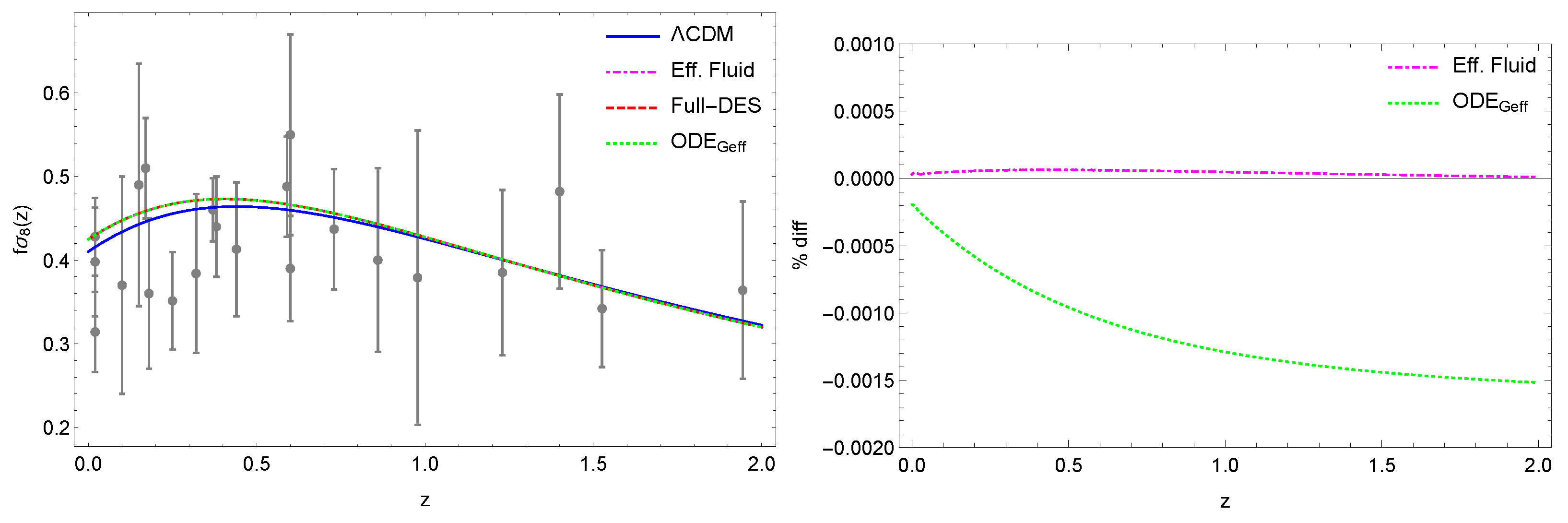
As a concrete example, we set , , , and , unless otherwise specified. Then we show the evolution of the growth-rate parameter for the HDES model on the left panel of Figure 2. Specifically, we show the “Full-DES” brute-force numerical solution, the effective fluid approach, the CDM model and the numerical solution of the equation and as can be seen, the agreement between all approaches is excellent. On the other hand, in the right panel of Figure 2, we show the percent difference between the “Full-DES” brute-force numerical solution and the effective fluid approach (magenta dot dashed line) and the numerical solution of the growth factor Equation (39) (green dotted line).
3.3. Modifications to CLASS and the ISW Effect
Finally, we now show how the effective fluid approach can be implemented into a Boltzmann code, such as CLASS [69]. Our modifications to the code are denoted as EFCLASS [97,108], while we also compare with the hi_CLASS code [113], which solves the full set of dynamical equations, but at the cost of significantly more complicated modifications.
In our case, however, the modifications for the effective fluid approach are much easier, as we only require the DE velocity and the anisotropic stress [97,108]. In the particular case where we consider the HDES model, then there is the further simplification that the anisotropic stress is also zero, as can be seen from Equation (109), since . Thus, to modify CLASS, we only require the expression for the DE velocity, which for is given by
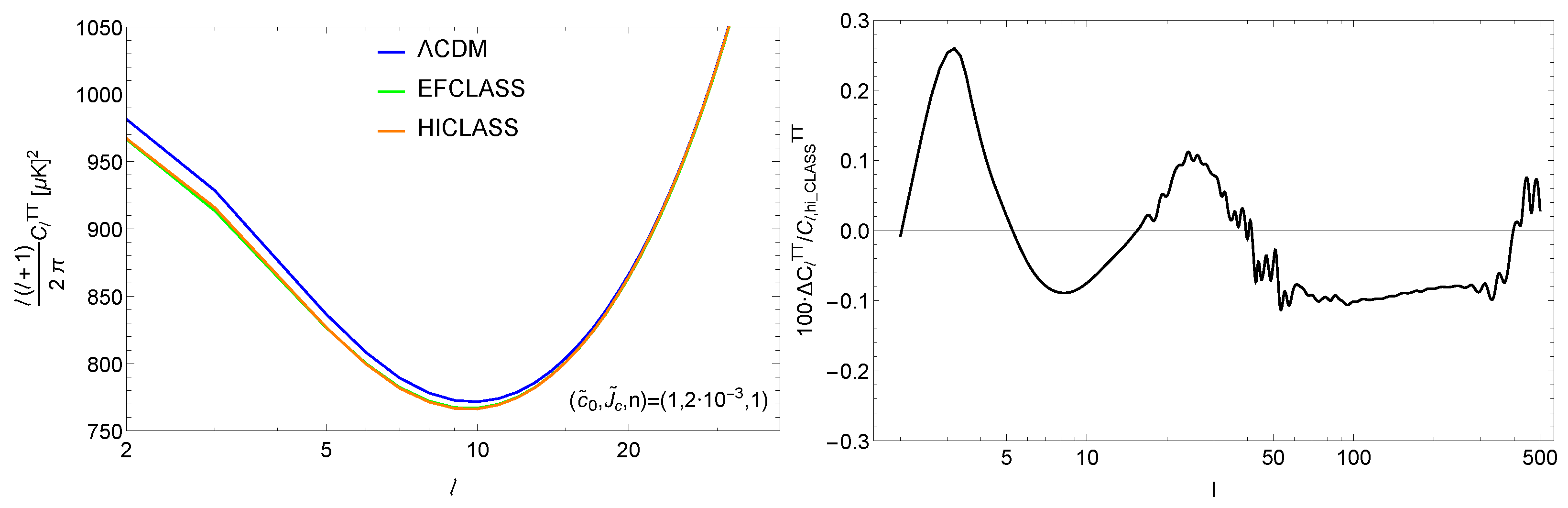
Next, we show the results of applying Equation (150) to the CLASS code and comparing with hi_CLASS. This is shown in the left panel of Figure 3, where the low-ℓ multipoles of the TT CMB spectrum for a flat universe with , , , and can be seen. Our EFCLASS code is denoted by the green line, hi_CLASS is given by the orange line, while the blue line corresponds to the CDM model. As can be seen, the agreement between EFCLASS and hi_CLASS is remarkable and even with our simple modification, has roughly accuracy across all multipoles (shown on the right panel of Figure 3).
Finally, we also compare our modifications of the effective fluid approach with a direct calculation of the integrated Sachs–Wolfe (ISW) effect. Specifically, the temperature power spectrum is given by [114]
where is a kernel that depends on the line of sight integral of the growth and a bessel function, while is the primordial power spectrum, given by the primordial power spectrum times a transfer function [97,114]
where is the primordial amplitude, is the pivot scale and is the Bardeen, Bond, Kaiser and Szalay (BBKS) transfer function [115].
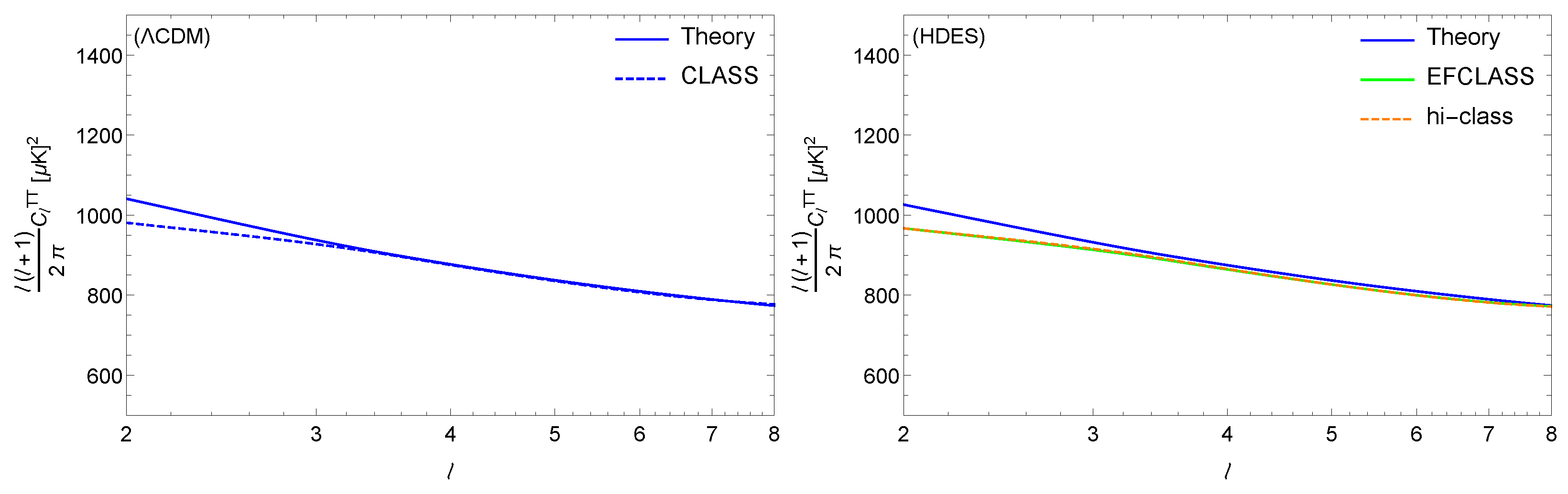
We show in Figure 4 a comparison between CLASS and hi_CLASS for the CDM model (left) and the HDES models (right), for the same parameters as in Figure 3. Overall, there is good agreement at all multipoles, except for , as the BBKS formula is only accurate on large scales or equivalently, small multipoles.
4. Conclusions
In this review, we briefly presented the so-called effective fluid approach, which is a framework that allows for treating modified gravity models as GR with an ideal DE fluid, described by an equation of state, a sound speed, an anisotropic stress and DE pressure, density and velocity perturbations. While in general MG models have very complicated evolution equations, they are significantly simplified under the effective fluid approach with the addition of the quasi-static and sub-horizon approximations, as they can be written in terms simple DE fluid equations. However, it should noted that in general it is not possible to discriminate modified gravity models from GR plus DE exotic fluids, as one may always move the modifications of gravity to the right-hand side of the field equations and rewrite them as the Einstein equations with extra matter/DE contributions.
Thus, the main advantage of this approach, as highlighted in this work, is that it allows us to easily including most MG models in the Boltzmann codes, as the latter are typically fine-tuned and hard-coded for GR and a DE fluid. Here, we presented the main formalism and the results for the DE fluid quantities for several MG models, including the , Horndeski and scalar–vector–tensor models, in all of which we presented the critical quantities that describe the evolution of the perturbations and the effective DE fluid equations.
We also described some specific applications, i.e., the numerical solutions of the fluid equations for growth factor, the designer Horndeski model and how our approach can be implemented in the Boltzmann codes. In the case of the HDES model, we found that with our effective fluid approach and just a simple modification, the agreement between our modified EFCLASS code and the more complicated, but exact, hi_CLASS code, is roughly ∼0.1% accuracy across all multipoles, as shown on the right panel of Figure 3.
Finally, we should also stress that an open point of debate in the community is the proper application of the quasi-static approximation, especially in more complicated models, as is extensively discussed in Ref. [116]. Even though this issue does not affect our effective fluid approach, it is a point that should be addressed prior to the advent of the next-generation surveys, in order to avoid unwanted theoretical errors in the predictions. Still, as demonstrated in this work, the effective fluid approach can provide a powerful framework, covering most viable MG models and allowing for a simple (and educational) way to modify the Boltzmann codes, which are necessary in data analyses.
Funding
S.N. acknowledges support from the research project PID2021-123012NB-C43, and the Spanish Research Agency (Agencia Estatal de Investigación) through the Grant IFT Centro de Excelencia Severo Ochoa No CEX2020-001007-S, funded by MCIN/AEI/10.13039/501100011033.
Institutional Review Board Statement
Not applicable.
Informed Consent Statement
Not applicable.
Data Availability Statement
Not applicable.
Conflicts of Interest
The authors declare no conflict of interest.
Abbreviations
The following abbreviations are used in this manuscript:
| BBKS | Bardeen, Bond, Kaiser and Szalay (transfer function) |
| CAMB | Code for Anisotropies in the Microwave Background |
| CDM | Cold Dark Matter |
| CLASS | Cosmic Linear Anisotropy Solving System |
| CMB | Cosmic Microwave Background |
| DE | Dark Energy |
| DM | Dark Matter |
| EFCLASS | Effective Fluid CLASS |
| EOS | Equation of State |
| FLRW | Friedmann–Lemaître–Robertson–Walker metric |
| GC | Galaxy Counts |
| GR | General Relativity |
| GW | Gravitational Wave |
| ISW | Integrated Sachs-Wolfe effect |
| HDES | Horndeski Designer model |
| HS | Hu–Sawicki model |
| KGB | Kinetic Gravity Braiding model |
| CDM | The cosmological constant () and cold dark matter (CDM) model |
| LSS | Large-Scale Structure |
| MG | Modified Gravity |
| SVT | Scalar–Vector–Tensor |
| 1 | In this review, our conventions are: (-+++) for the metric signature, the Riemann and Ricci tensors are given by and . The Einstein equations are for and is the bare Newton’s constant, while in what follows, we set the speed of light . |
| 2 | For the sake of brevity, we now set in what follows , and where . |
References
- Riess, A.G. et al. [The American Astronomical Society] Observational evidence from supernovae for an accelerating universe and a cosmological constant. Astron. J. 1998, 116, 1009–1038. [Google Scholar] [CrossRef] [Green Version]
- Perlmutter, S. et al. [The American Astronomical Society] Measurements of Omega and Lambda from 42 high redshift supernovae. Astrophys. J. 1999, 517, 565–586. [Google Scholar] [CrossRef]
- Kofman, L.; Starobinsky, A.A. Effect of the cosmological constant on large scale anisotropies in the microwave backbround. Sov. Astron. Lett. 1985, 11, 271–274. [Google Scholar]
- Aghanim, N. et al. [Planck Collaboration] Planck 2018 results. VI. Cosmological parameters. Astron. Astrophys. 2020, 641, A6. [Google Scholar]
- Abbott, T.M.C. et al. [Dark Energy Survey Collaboration] Dark Energy Survey year 1 results: Cosmological constraints from galaxy clustering and weak lensing. Phys. Rev. D 2018, D98, 043526. [Google Scholar] [CrossRef] [Green Version]
- Weinberg, S. The Cosmological Constant Problem. Rev. Mod. Phys. 1989, 61, 569. [Google Scholar] [CrossRef]
- Carroll, S.M. The Cosmological constant. Living Rev. Rel. 2001, 4, 1. [Google Scholar] [CrossRef] [Green Version]
- Hinshaw, G. et al. [The American Astronomical Society] Nine-Year Wilkinson Microwave Anisotropy Probe (WMAP) Observations: Cosmological Parameter Results. Astrophys. J. Suppl. 2013, 208, 19. [Google Scholar] [CrossRef] [Green Version]
- Copeland, E.J.; Sami, M.; Tsujikawa, S. Dynamics of dark energy. Int. J. Mod. Phys. D 2006, 15, 1753–1936. [Google Scholar] [CrossRef] [Green Version]
- Ratra, B.; Peebles, P.J.E. Cosmological Consequences of a Rolling Homogeneous Scalar Field. Phys. Rev. D 1988, 37, 3406. [Google Scholar] [CrossRef]
- Armendariz-Picon, C.; Mukhanov, V.F.; Steinhardt, P.J. A Dynamical solution to the problem of a small cosmological constant and late time cosmic acceleration. Phys. Rev. Lett. 2000, 85, 4438–4441. [Google Scholar] [CrossRef] [PubMed] [Green Version]
- Clifton, T.; Ferreira, P.G.; Padilla, A.; Skordis, C. Modified Gravity and Cosmology. Phys. Rep. 2012, 513, 1–189. [Google Scholar] [CrossRef]
- Collett, T.E.; Oldham, L.J.; Smith, R.J.; Auger, M.W.; Westfall, K.B.; Bacon, D.; Nichol, R.C.; Masters, K.L.; Koyama, K.; van den Bosch, R. A precise extragalactic test of General Relativity. Science 2018, 360, 1342. [Google Scholar] [CrossRef] [PubMed] [Green Version]
- Abbott, B.P. et al. [LIGO Scientific and Virgo Collaborations] Tests of general relativity with GW150914. Phys. Rev. Lett. 2016, 116, 221101, Erratum in Phys. Rev. Lett. 2018, 121, 129902.. [Google Scholar] [CrossRef] [PubMed] [Green Version]
- Nesseris, S.; Shafieloo, A. A model independent null test on the cosmological constant. Mon. Not. Roy. Astron. Soc. 2010, 408, 1879–1885. [Google Scholar] [CrossRef] [Green Version]
- Nesseris, S.; Garcia-Bellido, J. A new perspective on Dark Energy modeling via Genetic Algorithms. JCAP 2012, 1211, 033. [Google Scholar] [CrossRef] [Green Version]
- Abbott, B.P. et al. [LIGO Scientific Collaboration and Virgo Collaboration] GW170814: A Three-Detector Observation of Gravitational Waves from a Binary Black Hole Coalescence. Phys. Rev. Lett. 2017, 119, 141101. [Google Scholar] [CrossRef] [Green Version]
- Creminelli, P.; Vernizzi, F. Dark Energy after GW170817 and GRB170817A. Phys. Rev. Lett. 2017, 119, 251302. [Google Scholar] [CrossRef] [Green Version]
- Sakstein, J.; Jain, B. Implications of the Neutron Star Merger GW170817 for Cosmological Scalar-Tensor Theories. Phys. Rev. Lett. 2017, 119, 251303. [Google Scholar] [CrossRef] [Green Version]
- Ezquiaga, J.M.; Zumalacarregui, M. Dark Energy After GW170817: Dead Ends and the Road Ahead. Phys. Rev. Lett. 2017, 119, 251304. [Google Scholar] [CrossRef] [Green Version]
- Baker, T.; Bellini, E.; Ferreira, P.G.; Lagos, M.; Noller, J.; Sawicki, I. Strong constraints on cosmological gravity from GW170817 and GRB 170817A. Phys. Rev. Lett. 2017, 119, 251301. [Google Scholar] [CrossRef] [PubMed] [Green Version]
- Amendola, L.; Kunz, M.; Saltas, I.D.; Sawicki, I. Fate of Large-Scale Structure in Modified Gravity After GW170817 and GRB170817A. Phys. Rev. Lett. 2018, 120, 131101. [Google Scholar] [CrossRef] [PubMed]
- Crisostomi, M.; Koyama, K. Self-accelerating universe in scalar-tensor theories after GW170817. Phys. Rev. D 2018, 97, 084004. [Google Scholar] [CrossRef] [Green Version]
- Frusciante, N.; Peirone, S.; Casas, S.; Lima, N.A. Cosmology of surviving Horndeski theory: The road ahead. Phys. Rev. D 2019, 99, 063538. [Google Scholar] [CrossRef] [Green Version]
- Kase, R.; Tsujikawa, S. Dark energy in Horndeski theories after GW170817: A review. Int. J. Mod. Phys. D 2019, 28, 1942005. [Google Scholar] [CrossRef] [Green Version]
- McManus, R.; Lombriser, L.; Peñarrubia, J. Finding Horndeski theories with Einstein gravity limits. JCAP 2016, 1611, 006. [Google Scholar] [CrossRef]
- Lombriser, L.; Taylor, A. Breaking a Dark Degeneracy with Gravitational Waves. JCAP 2016, 1603, 031. [Google Scholar] [CrossRef] [Green Version]
- Sotiriou, T.P.; Faraoni, V. f(R) Theories Of Gravity. Rev. Mod. Phys. 2010, 82, 451–497. [Google Scholar] [CrossRef] [Green Version]
- De Felice, A.; Tsujikawa, S. f(R) theories. Living Rev. Rel. 2010, 13, 3. [Google Scholar] [CrossRef] [Green Version]
- Nojiri, S.; Odintsov, S.D.; Oikonomou, V.K. Modified Gravity Theories on a Nutshell: Inflation, Bounce and Late-time Evolution. Phys. Rep. 2017, 692, 1–104. [Google Scholar] [CrossRef] [Green Version]
- Nojiri, S.; Odintsov, S.D. Unified cosmic history in modified gravity: From F(R) theory to Lorentz non-invariant models. Phys. Rep. 2011, 505, 59–144. [Google Scholar] [CrossRef] [Green Version]
- Multamaki, T.; Vilja, I. Cosmological expansion and the uniqueness of gravitational action. Phys. Rev. D 2006, 73, 024018. [Google Scholar] [CrossRef]
- De la Cruz-Dombriz, A.; Dobado, A. A f(R) gravity without cosmological constant. Phys. Rev. D 2006, 74, 087501. [Google Scholar] [CrossRef] [Green Version]
- Pogosian, L.; Silvestri, A. The pattern of growth in viable f(R) cosmologies. Phys. Rev. D 2008, 77, 023503, Erratum in Phys. Rev. D 2010, 81, 049901.. [Google Scholar] [CrossRef] [Green Version]
- Nesseris, S. Can the degeneracies in the gravity sector be broken? Phys. Rev. D 2013, 88, 123003. [Google Scholar] [CrossRef] [Green Version]
- Tsujikawa, S. Matter density perturbations and effective gravitational constant in modified gravity models of dark energy. Phys. Rev. D 2007, 76, 023514. [Google Scholar] [CrossRef] [Green Version]
- Nesseris, S.; Sapone, D. Accuracy of the growth index in the presence of dark energy perturbations. Phys. Rev. D 2015, 92, 023013. [Google Scholar] [CrossRef] [Green Version]
- Luna, C.A.; Basilakos, S.; Nesseris, S. Cosmological constraints on γ-gravity models. Phys. Rev. D 2018, 98, 023516. [Google Scholar] [CrossRef] [Green Version]
- Perez-Romero, J.; Nesseris, S. Cosmological constraints and comparison of viable f(R) models. Phys. Rev. D 2018, 97, 023525. [Google Scholar] [CrossRef] [Green Version]
- Hu, W.; Sawicki, I. Models of f(R) Cosmic Acceleration that Evade Solar-System Tests. Phys. Rev. D 2007, 76, 064004. [Google Scholar] [CrossRef] [Green Version]
- Hu, W.; Sawicki, I. A Parameterized Post-Friedmann Framework for Modified Gravity. Phys. Rev. D 2007, 76, 104043. [Google Scholar] [CrossRef] [Green Version]
- Kunz, M.; Sapone, D. Dark Energy versus Modified Gravity. Phys. Rev. Lett. 2007, 98, 121301. [Google Scholar] [CrossRef] [PubMed]
- Koivisto, T.; Mota, D.F. Cosmology and Astrophysical Constraints of Gauss-Bonnet Dark Energy. Phys. Lett. B 2007, 644, 104–108. [Google Scholar] [CrossRef] [Green Version]
- Koivisto, T.; Mota, D.F. Gauss-Bonnet Quintessence: Background Evolution, Large Scale Structure and Cosmological Constraints. Phys. Rev. D 2007, 75, 023518. [Google Scholar] [CrossRef] [Green Version]
- De la Cruz-Dombriz, A.; Dobado, A.; Maroto, A.L. On the evolution of density perturbations in f(R) theories of gravity. Phys. Rev. D 2008, 77, 123515. [Google Scholar] [CrossRef] [Green Version]
- Starobinsky, A.A. Disappearing cosmological constant in f(R) gravity. JETP Lett. 2007, 86, 157–163. [Google Scholar] [CrossRef] [Green Version]
- Bean, R.; Bernat, D.; Pogosian, L.; Silvestri, A.; Trodden, M. Dynamics of Linear Perturbations in f(R) Gravity. Phys. Rev. D 2007, 75, 064020. [Google Scholar] [CrossRef] [Green Version]
- Song, Y.S.; Hollenstein, L.; Caldera-Cabral, G.; Koyama, K. Theoretical Priors On Modified Growth Parametrisations. JCAP 2010, 1004, 018. [Google Scholar] [CrossRef] [Green Version]
- Pogosian, L.; Silvestri, A.; Koyama, K.; Zhao, G.B. How to optimally parametrize deviations from General Relativity in the evolution of cosmological perturbations? Phys. Rev. D 2010, 81, 104023. [Google Scholar] [CrossRef] [Green Version]
- Bean, R.; Tangmatitham, M. Current constraints on the cosmic growth history. Phys. Rev. D 2010, 81, 083534. [Google Scholar] [CrossRef] [Green Version]
- Caldwell, R.; Cooray, A.; Melchiorri, A. Constraints on a New Post-General Relativity Cosmological Parameter. Phys. Rev. D 2007, 76, 023507. [Google Scholar] [CrossRef] [Green Version]
- Bertschinger, E.; Zukin, P. Distinguishing Modified Gravity from Dark Energy. Phys. Rev. D 2008, 78, 024015. [Google Scholar] [CrossRef]
- Baker, T.; Ferreira, P.G.; Skordis, C.; Zuntz, J. Towards a fully consistent parameterization of modified gravity. Phys. Rev. D 2011, 84, 124018. [Google Scholar] [CrossRef] [Green Version]
- Silvestri, A.; Pogosian, L.; Buniy, R.V. Practical approach to cosmological perturbations in modified gravity. Phys. Rev. D 2013, 87, 104015. [Google Scholar] [CrossRef] [Green Version]
- Clifton, T.; Sanghai, V.A.A. Parameterizing theories of gravity on large and small scales in cosmology. Phys. Rev. Lett. 2019, 122, 011301. [Google Scholar] [CrossRef] [Green Version]
- Ishak, M. Testing General Relativity in Cosmology. Living Rev. Relativ. 2019, 22, 1. [Google Scholar] [CrossRef] [Green Version]
- Zhao, G.B.; Pogosian, L.; Silvestri, A.; Zylberberg, J. Searching for modified growth patterns with tomographic surveys. Phys. Rev. D 2009, 79, 083513. [Google Scholar] [CrossRef] [Green Version]
- Lewis, A.; Challinor, A.; Lasenby, A. Efficient computation of CMB anisotropies in closed FRW models. Astrophys. J 2000, 538, 473–476. [Google Scholar] [CrossRef] [Green Version]
- Hojjati, A.; Pogosian, L.; Zhao, G.B. Testing gravity with CAMB and CosmoMC. JCAP 2011, 1108, 005. [Google Scholar] [CrossRef] [Green Version]
- He, J.h. Testing f(R) dark energy model with the large scale structure. Phys. Rev. D 2012, 86, 103505. [Google Scholar] [CrossRef] [Green Version]
- Xu, L. FRCAMB: An f(R) Code for Anisotropies in the Microwave Background. arXiv 2015, arXiv:1506.03232. [Google Scholar]
- Gubitosi, G.; Piazza, F.; Vernizzi, F. The Effective Field Theory of Dark Energy. JCAP 2013, 1302, 032. [Google Scholar] [CrossRef] [Green Version]
- Hu, B.; Raveri, M.; Frusciante, N.; Silvestri, A. Effective Field Theory of Cosmic Acceleration: An implementation in CAMB. Phys. Rev. D 2014, 89, 103530. [Google Scholar] [CrossRef]
- Ade, P.A.R. et al. [Planck Collaboration] Planck 2015 results. XIV. Dark energy and modified gravity. Astron. Astrophys. 2016, 594, A14. [Google Scholar] [CrossRef] [Green Version]
- Battye, R.A.; Bolliet, B.; Pearson, J.A. f(R) gravity as a dark energy fluid. Phys. Rev. D 2016, 93, 044026. [Google Scholar] [CrossRef] [Green Version]
- Capozziello, S.; Nojiri, S.; Odintsov, S.D. Dark energy: The Equation of state description versus scalar-tensor or modified gravity. Phys. Lett. B 2006, 634, 93–100. [Google Scholar] [CrossRef] [Green Version]
- Capozziello, S.; Nojiri, S.; Odintsov, S.D.; Troisi, A. Cosmological viability of f(R)-gravity as an ideal fluid and its compatibility with a matter dominated phase. Phys. Lett. B 2006, 639, 135–143. [Google Scholar] [CrossRef] [Green Version]
- Capozziello, S.; Mantica, C.A.; Molinari, L.G. Cosmological perfect-fluids in f(R) gravity. Int. J. Geom. Meth. Mod. Phys. 2019, 16, 1950008. [Google Scholar] [CrossRef] [Green Version]
- Blas, D.; Lesgourgues, J.; Tram, T. The Cosmic Linear Anisotropy Solving System (CLASS) II: Approximation schemes. JCAP 2011, 1107, 034. [Google Scholar] [CrossRef] [Green Version]
- Battye, R.A.; Bolliet, B.; Pace, F. Do cosmological data rule out f(R) with w≠-1? Phys. Rev. D 2018, 97, 104070. [Google Scholar] [CrossRef] [Green Version]
- Kunz, M. The phenomenological approach to modeling the dark energy. C. R. Phys. 2012, 13, 539–565. [Google Scholar] [CrossRef] [Green Version]
- Saltas, I.D.; Kunz, M. Anisotropic stress and stability in modified gravity models. Phys. Rev. D 2011, 83, 064042. [Google Scholar] [CrossRef] [Green Version]
- Sawicki, I.; Bellini, E. Limits of quasistatic approximation in modified-gravity cosmologies. Phys. Rev. D 2015, 92, 084061. [Google Scholar] [CrossRef]
- Cardona, W.; Hollenstein, L.; Kunz, M. The traces of anisotropic dark energy in light of Planck. JCAP 2014, 1407, 032. [Google Scholar] [CrossRef] [Green Version]
- Koivisto, T.; Mota, D.F. Dark energy anisotropic stress and large scale structure formation. Phys. Rev. D 2006, 73, 083502. [Google Scholar] [CrossRef]
- Mota, D.F.; Kristiansen, J.R.; Koivisto, T.; Groeneboom, N.E. Constraining Dark Energy Anisotropic Stress. Mon. Not. R. Astron. Soc. 2007, 382, 793–800. [Google Scholar] [CrossRef] [Green Version]
- Hu, W. Structure formation with generalized dark matter. Astrophys. J. 1998, 506, 485–494. [Google Scholar] [CrossRef] [Green Version]
- De Putter, R.; Huterer, D.; Linder, E.V. Measuring the Speed of Dark: Detecting Dark Energy Perturbations. Phys. Rev. D 2010, 81, 103513. [Google Scholar] [CrossRef] [Green Version]
- Batista, R.C.; Marra, V. Clustering dark energy and halo abundances. JCAP 2017, 1711, 048. [Google Scholar] [CrossRef] [Green Version]
- Lewis, A.; Bridle, S. Cosmological parameters from CMB and other data: A Monte Carlo approach. Phys. Rev. D 2002, 66, 103511. [Google Scholar] [CrossRef] [Green Version]
- Tegmark, M. et al. [the SDSS collaboration] Cosmological parameters from SDSS and WMAP. Phys. Rev. D 2004, 69, 103501. [Google Scholar] [CrossRef] [Green Version]
- Ade, P.A.R. et al. [Planck Collaboration] Planck 2015 results. XIII. Cosmological parameters. Astron. Astrophys. 2016, 594, A13. [Google Scholar] [CrossRef] [Green Version]
- Zhao, G.B.; Raveri, M.; Pogosian, P.; Wang, Y.; Crittenden, R.G.; Handley, W.J.; Percival, W.J.; Beutler, F.; Brinkmann, J.; Chuang, C.; et al. Dynamical dark energy in light of the latest observations. Nat. Astron. 2017, 1, 627–632. [Google Scholar] [CrossRef]
- Heavens, A.; Fantaye, Y.; Sellentin, E.; Eggers, H.; Hosenie, Z.; Kroon, S.; Mootoovaloo, A. No evidence for extensions to the standard cosmological model. Phys. Rev. Lett. 2017, 119, 101301. [Google Scholar] [CrossRef] [PubMed] [Green Version]
- Freedman, W.L. Cosmology at a Crossroads. Nat. Astron. 2017, 1, 0121. [Google Scholar] [CrossRef]
- Renk, J.; Zumalacarregui, M.; Montanari, F.; Barreira, A. Galileon gravity in light of ISW, CMB, BAO and H0 data. JCAP 2017, 1710, 020. [Google Scholar] [CrossRef] [Green Version]
- Nunes, R.C. Structure formation in f(T) gravity and a solution for H0 tension. JCAP 2018, 1805, 052. [Google Scholar] [CrossRef] [Green Version]
- Lin, M.X.; Raveri, M.; Hu, W. Phenomenology of Modified Gravity at Recombination. Phys. Rev. D 2019, 99, 043514. [Google Scholar] [CrossRef] [Green Version]
- Benetti, M.; Santos da Costa, S.; Capozziello, S.; Alcaniz, J.S.; De Laurentis, M. Observational constraints on Gauss? Bonnet cosmology. Int. J. Mod. Phys. D 2018, 27, 1850084. [Google Scholar] [CrossRef] [Green Version]
- Sakr, Z.; Ilic, S.; Blanchard, A. Cluster counts: Calibration issue or new physics? Astron. Astrophys. 2018, 620, A78. [Google Scholar] [CrossRef] [Green Version]
- Ma, C.P.; Bertschinger, E. Cosmological perturbation theory in the synchronous and conformal Newtonian gauges. Astrophys. J. 1995, 455, 7–25. [Google Scholar] [CrossRef] [Green Version]
- Amendola, L.; Tsujikawa, S. Dark Energy; Cambridge University Press: Cambridge, UK, 2015. [Google Scholar]
- Mukhanov, V.F.; Feldman, H.A.; Brandenberger, R.H. Theory of cosmological perturbations. Part 1. Classical perturbations. Part 2. Quantum theory of perturbations. Part 3. Extensions. Phys. Rept. 1992, 215, 203–333. [Google Scholar] [CrossRef] [Green Version]
- Sapone, D.; Kunz, M. Fingerprinting Dark Energy. Phys. Rev. D 2009, 80, 083519. [Google Scholar] [CrossRef]
- Nesseris, S.; Perivolaropoulos, L. Crossing the Phantom Divide: Theoretical Implications and Observational Status. JCAP 2007, 0701, 018. [Google Scholar] [CrossRef]
- Wald, R.M. General Relativity; Chicago Univ. Pr.: Chicago, IL, USA, 1984. [Google Scholar] [CrossRef]
- Arjona, R.; Cardona, W.; Nesseris, S. Unraveling the effective fluid approach for f(R) models in the subhorizon approximation. Phys. Rev. D 2019, 99, 043516. [Google Scholar] [CrossRef] [Green Version]
- Horndeski, G.W. Second-order scalar-tensor field equations in a four-dimensional space. Int. J. Theor. Phys. 1974, 10, 363–384. [Google Scholar] [CrossRef]
- Abbott, B.P. et al. [The American Astronomical Society] Gravitational Waves and Gamma-rays from a Binary Neutron Star Merger: GW170817 and GRB 170817A. Astrophys. J. Lett. 2017, 848, L13. [Google Scholar] [CrossRef] [Green Version]
- Kobayashi, T.; Yamaguchi, M.; Yokoyama, J. Generalized G-inflation: Inflation with the most general second-order field equations. Prog. Theor. Phys. 2011, 126, 511–529. [Google Scholar] [CrossRef]
- Chiba, T. 1/R gravity and scalar-tensor gravity. Phys. Lett. B 2003, 575, 1–3. [Google Scholar] [CrossRef] [Green Version]
- Brans, C.; Dicke, R.H. Mach’s principle and a relativistic theory of gravitation. Phys. Rev. 1961, 124, 925–935. [Google Scholar] [CrossRef]
- Deffayet, C.; Pujolas, O.; Sawicki, I.; Vikman, A. Imperfect Dark Energy from Kinetic Gravity Braiding. JCAP 2010, 10, 026. [Google Scholar] [CrossRef]
- Quiros, I. Selected topics in scalar–tensor theories and beyond. Int. J. Mod. Phys. D 2019, 28, 1930012. [Google Scholar] [CrossRef]
- Kimura, R.; Yamamoto, K. Large Scale Structures in Kinetic Gravity Braiding Model That Can Be Unbraided. JCAP 2011, 1104, 025. [Google Scholar] [CrossRef] [Green Version]
- De Felice, A.; Kobayashi, T.; Tsujikawa, S. Effective gravitational couplings for cosmological perturbations in the most general scalar-tensor theories with second-order field equations. Phys. Lett. B 2011, 706, 123–133. [Google Scholar] [CrossRef] [Green Version]
- Matsumoto, J. Oscillating solutions of the matter density contrast in Horndeski’s theory. JCAP 2019, 1901, 054. [Google Scholar] [CrossRef] [Green Version]
- Arjona, R.; Cardona, W.; Nesseris, S. Designing Horndeski and the effective fluid approach. Phys. Rev. D 2019, 100, 063526. [Google Scholar] [CrossRef] [Green Version]
- Heisenberg, L.; Kase, R.; Tsujikawa, S. Cosmology in scalar-vector-tensor theories. Phys. Rev. D 2018, 98, 024038. [Google Scholar] [CrossRef] [Green Version]
- Cardona, W.; Orjuela-Quintana, J.B.; Valenzuela-Toledo, C.A. An effective fluid description of scalar-vector-tensor theories under the sub-horizon and quasi-static approximations. JCAP 2022, 08, 059. [Google Scholar] [CrossRef]
- Linder, E.V. Horndessence: ΛCDM Cosmology from Modified Gravity. arXiv 2021, arXiv:2104.14560. [Google Scholar]
- Sagredo, B.; Nesseris, S.; Sapone, D. Internal Robustness of Growth Rate data. Phys. Rev. D 2018, 98, 083543. [Google Scholar] [CrossRef] [Green Version]
- Zumalacarregui, M.; Bellini, E.; Sawicki, I.; Lesgourgues, J.; Ferreira, P.G. hi_class: Horndeski in the Cosmic Linear Anisotropy Solving System. JCAP 2017, 1708, 019. [Google Scholar] [CrossRef] [Green Version]
- Song, Y.S.; Hu, W.; Sawicki, I. The Large Scale Structure of f(R) Gravity. Phys. Rev. D 2007, 75, 044004. [Google Scholar] [CrossRef] [Green Version]
- Dodelson, S. Modern Cosmology; Academic Press: Amsterdam, The Netherlands, 2003. [Google Scholar]
- Pace, F.; Battye, R.; Bellini, E.; Lombriser, L.; Vernizzi, F.; Bolliet, B. Comparison of different approaches to the quasi-static approximation in Horndeski models. JCAP 2021, 6, 017. [Google Scholar] [CrossRef]
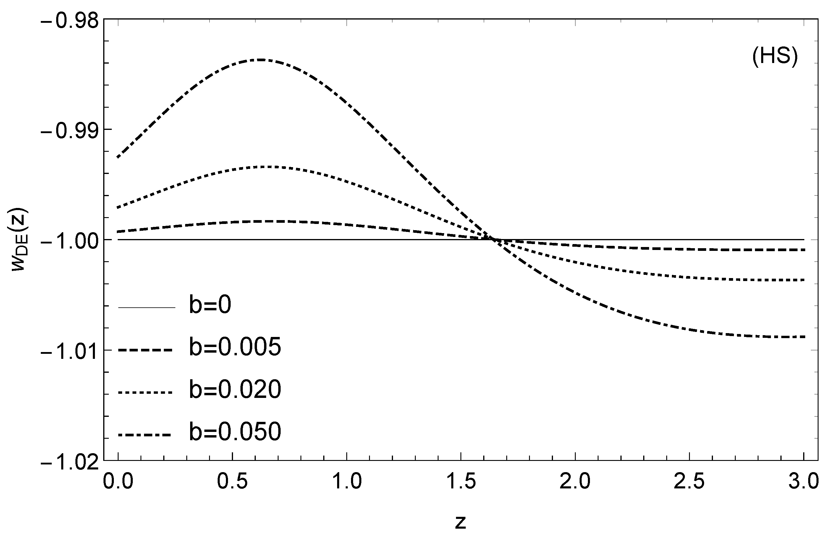
Figure 1.
The evolution of the effective DE equation of state for the HS model for , and various values of the b parameter which controls the deviations from the CDM model (see Ref. [97]), with . The equation of state crosses at , while at early times, we have , thus violating the SEC. Image from Ref. [97].

Figure 2.
(Left) The theoretical predictions for the parameter of the HDES model with , and versus the data compilation from Ref. [112]. (Right) The percent difference between the “Full-DES" brute-force numerical solution and the effective fluid approach (magenta dot dashed line) and the numerical solution of the growth factor equation (39) (green dotted line). Image from Ref. [108].

Figure 3.
(Left) The TT CMB spectrum for , , , and . The results of the EFCLASS code are denoted by the green line, those of hi_CLASS by an orange line and for the CDM with a blue line. (Right) The percent difference of our code with hi_CLASS. Image from Ref. [108].
Figure 3.
(Left) The TT CMB spectrum for , , , and . The results of the EFCLASS code are denoted by the green line, those of hi_CLASS by an orange line and for the CDM with a blue line. (Right) The percent difference of our code with hi_CLASS. Image from Ref. [108].


Disclaimer/Publisher’s Note: The statements, opinions and data contained in all publications are solely those of the individual author(s) and contributor(s) and not of MDPI and/or the editor(s). MDPI and/or the editor(s) disclaim responsibility for any injury to people or property resulting from any ideas, methods, instructions or products referred to in the content. |
© 2022 by the author. Licensee MDPI, Basel, Switzerland. This article is an open access article distributed under the terms and conditions of the Creative Commons Attribution (CC BY) license (https://creativecommons.org/licenses/by/4.0/).
Share and Cite
MDPI and ACS Style
Nesseris, S. The Effective Fluid Approach for Modified Gravity and Its Applications. Universe 2023, 9, 13. https://doi.org/10.3390/universe9010013
AMA Style
Nesseris S. The Effective Fluid Approach for Modified Gravity and Its Applications. Universe. 2023; 9(1):13. https://doi.org/10.3390/universe9010013
Chicago/Turabian StyleNesseris, Savvas. 2023. "The Effective Fluid Approach for Modified Gravity and Its Applications" Universe 9, no. 1: 13. https://doi.org/10.3390/universe9010013
Note that from the first issue of 2016, this journal uses article numbers instead of page numbers. See further details here.