
H0 Tension on the Light of Supermassive Black Hole Shadows Data


Abstract
:1. Introduction
- Measurements at low redshifts. SMBH shadows can be used to estimate in a cosmological independent way and also without evoking the distance ladder method. By adopting a peculiar velocity of the host galaxy in km/s, the mass of the SMBH M in solar masses and the angular size , we can directly compute the distance to the SMBH. Finally, using the Hubble law, we can estimate . Clearly, performing this kind of estimate using two SMBH shadows’ data points (M87* and Sgr A*) is insufficient, not only by the low data point density, but also due their high uncertainties. However, we expect a future improvement in this direction since the abundance of SMBHs can be hosted in spiral and elliptical galaxies [10]. At this scale, [11] proposed using a mock SMBH shadow catalog as anchor in the distance ladder method, which can offer an estimation of .
- Measurement at high redshifts. At this scale, determining the mass of the BH can be difficult due to the fact that we need high resolution in the equipment, and the estimation of the uncertainties is quite large. However, reverberation mappings [12] techniques combined with spectroastrometry analyses [13] have been employed to determine BH mass and distance simultaneously. In [14], the authors proposed a set of simulated SMBH shadows at this scale, which were performed by assuming a fiducial benchmark cosmology, making it possible to determine a set of cosmological parameters as and .
2. Black Hole Shadow Description as Standard Rulers
- Nearby galaxies (low redshift, ), where SMBH shadows are cosmologically model-independent and do not require methods that consider anchors in the distance ladder. By a simple calculation using the Hubble flow velocity of a galaxy and its peculiar velocity, we can derive the Hubble velocity and constrain . In addition, at , the angular size of the BH shadow grows as the BH mass gets bigger, which makes it a suitable candidate to study our local universe in comparison to the BAO peaks, in which amplitude decreases due to the cosmological expansion. However, since the angular size and the mass of the BH are linearly correlated, we require precise techniques to break this degeneracy such as, for example, stellar-dynamics [20], gas-dynamics [21] or maser observations [22,23].
- High(er) distance observations (high(er) redshift ()), where not only do we require a fiducial cosmology to determine the BH mass, but also we require an angular resolution around 0.1 as. These kinds of observations have been show to be extremely difficult [6]; however, by combining techniques such as reverberation mappings [12] and very long baseline interferometry technologies, it will be possible to achieve such resolution. Going further in distance, the search for quasars beyond [24] allows us to estimate BH masses at higher redshift. While the uncertainties in these measurements are high, it is important to note that this is a reference that SMBH shadows can be part of future catalogs, making them useful in proving the cosmic expansion at this scale.
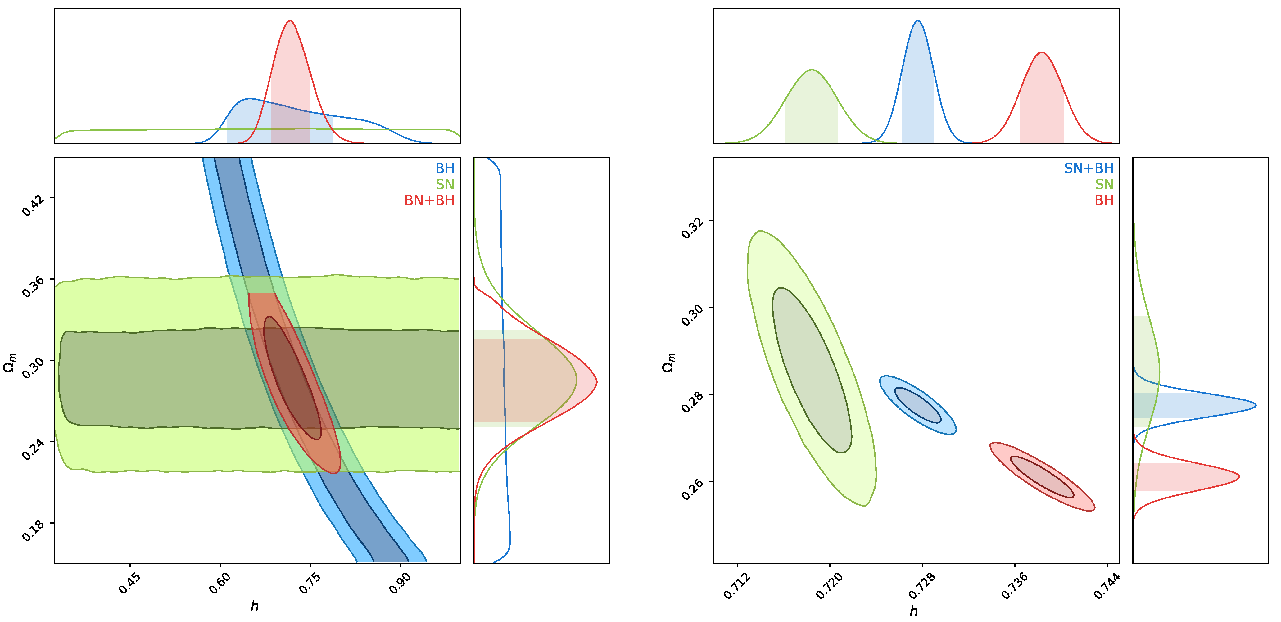
- Combination of M87 observation and SNIa catalog [14]. This proposal allows us to study a particular set of cosmological parameters by considering a collection of 10 BH shadows’ simulated data points under a fiducial benchmark cosmology ( and km/s/Mpc) and the Pantheon SNIa catalog (see Section 4 for its description). The results are reported in Table 2. However, these simulations are restricted solely to BH masses of within an interval , which, combined with SNIa observations, are not able to constrain the CDM model.
- Combination of mock catalogues for SMBH ( BH simulated data points) plus mock SNIa data for the Vera C. Rubin Observatory LSST2. This proposal starts from the same point of view as the latter; however, the mock SMBH data are used as anchors to calibrate the distance ladder. While the number of BH data points simulated is high, the forecasting is based on a benchmark cosmology and a single shadow data from M87. Furthermore, a cosmographic approach was employed at low redshift, making it impossible to constrain atthe third order of the series, i.e., the jerk current value [11].

| Base Line | Observable/Simulations | [km/s/Mpc] | |
|---|---|---|---|
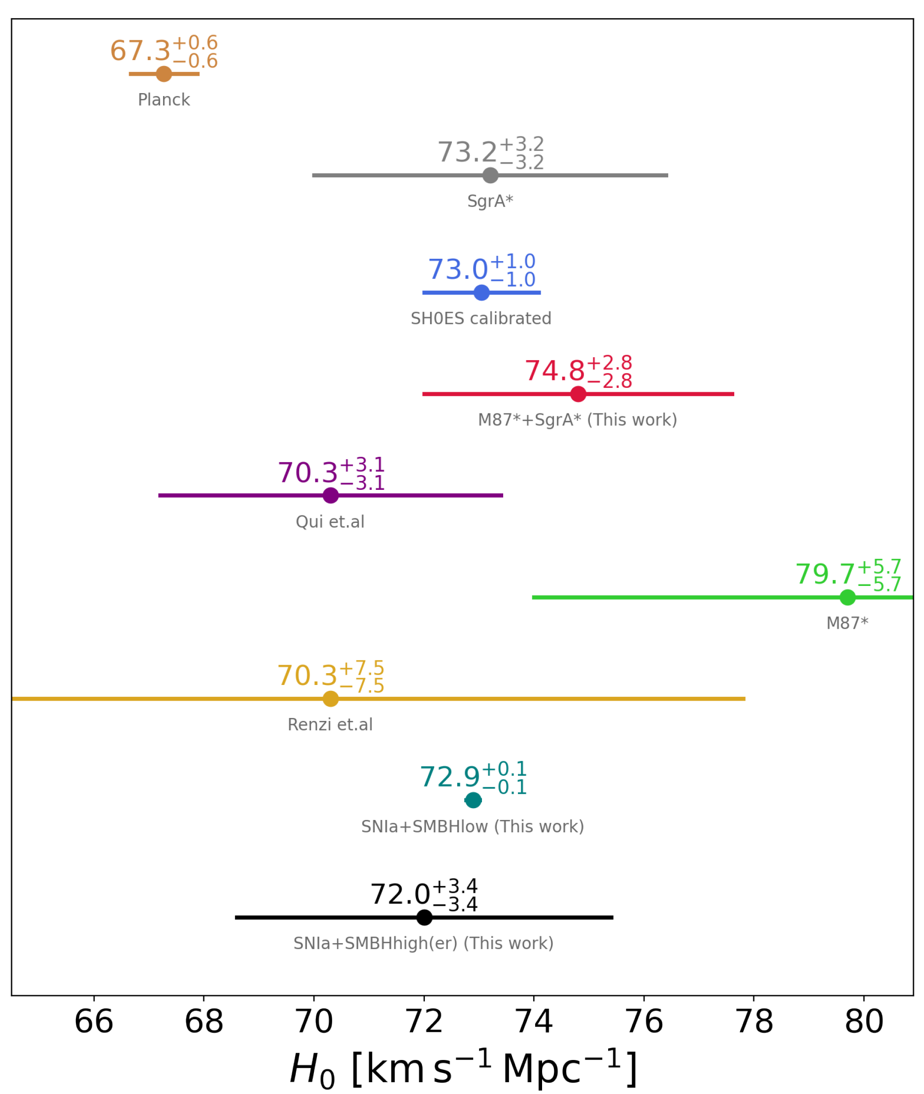
| Planck collaboration | CMB | 67.27 ± 0.604 | 0.315 ± 0.007 |
| SH0ES collaboration | Cepheid-SNIa sample with fixed | 73.04 ± 1.04 | |
| EHT first observations | Size of M87* shadow. | 79.7 ± 5.7 | - |
| EHT second Observations | Size of Sgr A* shadow. | 73.2 ± 3.2 | - |
| Both EHT Observations [This work] | Sizes of M87* and Sgr A* shadows. | 74.8 ± 2.8 | - |
| Qi et al. | Size of M87* shadow with a fixed mass using stellar-dynamics method plus SNIa from Pantheon catalog | 70.3 ± 3.1 | 0.301 ± 0.022 |
| Renzi et al. | Size of M87* shadow and mock catalogues for Supermassive BH ( BH simulated) plus mock SNIa data for LSST. | Fixed | |
| SNIa + SMBH at low redshift [This work] | Sizes of M87* and Sgr A* shadows, SNIa from Pantheon catalog plus forecasting for the sizes of SMBH shadows with M = at (see Section 3.2). | 72.89 ± 0.12 | 0.275 ± 0.002 |
| SNIa + SMBH at high redshift [This work] | SNIa from Pantheon catalog plus forecasting for the size of the SMBH shadows with M = between (see Section 3.1). | 72.0 ± 3.4 | 0.285 ± 0.029 |
3. Black Hole Shadows Forecasting
- Assume a conservative fiducial cosmological model. In our case, instead of using a conservative Planck data cosmology [28] as in other studies, we will consider the local values: km/s/Mpc, , where .
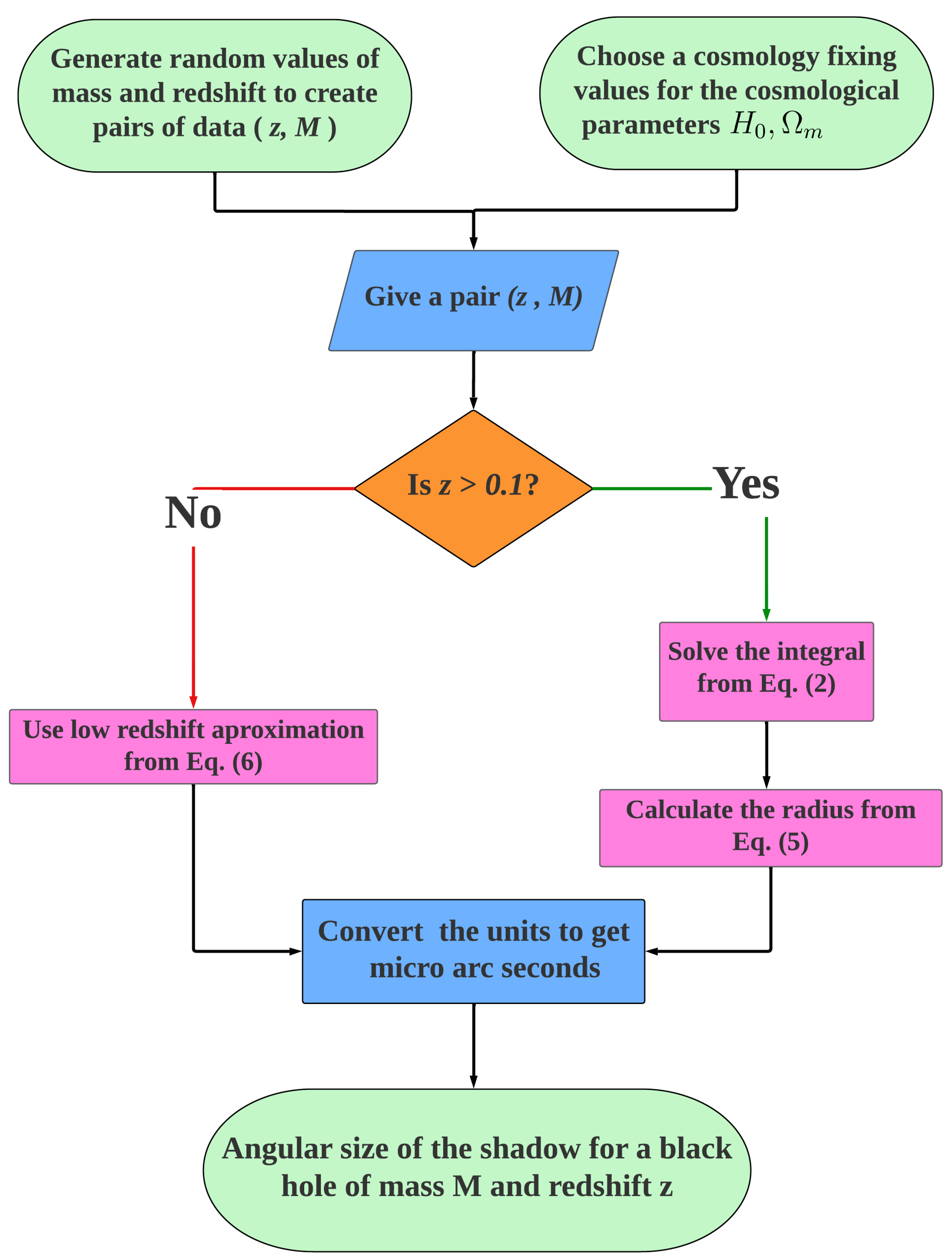
- Under the above condition, we compute Equation (2) only as a function of the redshift z. Once the integral is solved, we can use the reciprocity relation Equation (3) in Equation (5). This will be our main function, and it takes as input values a set of two variables: the redshift z and the SMBH mass. We can consider this result for the low redshift case as a cutoff when . Notice that it is necessary to write these equations in BH shadow units, e.g., , and perform the appropriate conversion to express the results in as units. Additionally, we need to assume an error in the simulations. In [14], the authors considered the M87* single data, which at low redshift constrains with a 13% error. In order to reduce this number, it was considered a symmetric uncertainty in this single data point as the variance takes the form ; therefore, if we want to reach a precision of , we require SMBH shadows simulations. While this assumption is reasonable and the estimated error decreases by almost 8%, the mean value for does not change. Since we are going to consider two SMBH shadows from M87* and Sgr A*, this symmetric uncertainty assumption will be relaxed in order to reach a precision of 4% using a conservative quantity comparable with other observables at low z, e.g., SNIa, and a number of simulations derived from data with asymmetric errors at high z.
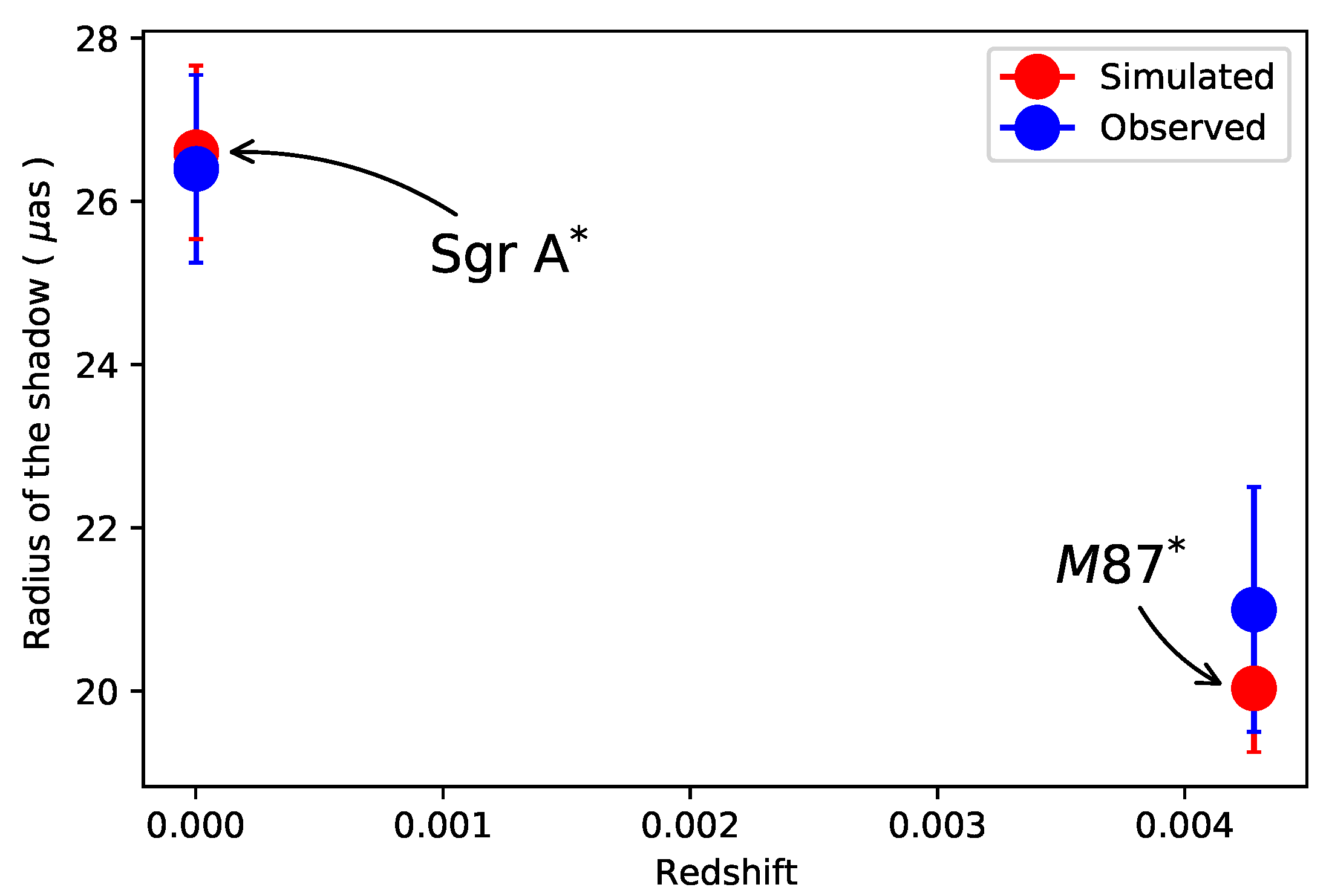
- In comparison to the previous methodologies described in Section 2, in order to test our algorithm effectiveness, we can compare the simulated SMBH shadows’ outputs with the current M87 and Sgr A* observations given by the EHT. As we show in Figure 1, the simulations are very near to the observables, e.g., for Sgr A* we have that as, while as. For the M87* case, we have a value as, and our simulation gives as. The latter result gives a 4.7% difference from the simulated data point. This quantity is due to our pre-established precision since the error percentage in the M87* observation is close to 7%, while for Sgr A* it is reduced to almost 4%.
3.1. High(er) Redshift Observations for Hubble Constant Constraints
3.2. Nearby Galaxies Estimation Observations for Hubble Constant Constraints
4. Current and Simulated Data Sets
- Pantheon SNIa catalog [29]. This catalog contains data of 1048 SNIa, observed in the range of low redshift from . For each supernova, the redshift z and the apparent magnitude are given, which allows us to build the modulus distance by fixing the absolute magnitude M. In this analysis, we use the value , for one case.
- EHT direct observations. This set contains data from the two observations of the SMBH M87* and Sgr A*. For each observable, their mass m is given in units, the redshift z and the radius of their shadow in as units. A compilation of these data is given in Table 1.
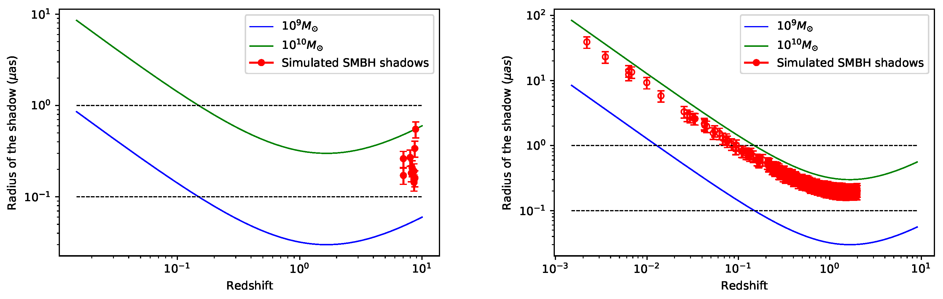
- High redshift SMBH shadows. This set contains 10 simulated shadows for SMBH between (see Figure 3 at the left). For each forecasted BH, its redshift z, the size of its radius in as and the error in this radius are given. Details are described in Section 3.1.
- Low redshift SMBH shadows. This set contains 500 simulated shadows for SMBH between (see Figure 3 at the right). For each forecasted BH its redshift z, the size of its radius in as and the error in this radius are given. Details are described in Section 3.2.
5. Results
6. Discussion
Author Contributions
Funding
Data Availability Statement
Acknowledgments
Conflicts of Interest
| 1 | |
| 2 | www.lsst.org accessed on 10 November 2022. |
| 3 | eventhorizontelescope.org accessed on 10 November 2022. |
| 4 | phoebe-project.org accessed on 10 November 2022. |
| 5 | getdist.readthedocs.io accessed on 10 November 2022. |
References
- Riess, A.G.; Yuan, W.; Macri, L.M. A Comprehensive Measurement of the Local Value of the Hubble Constant with 1 km/s/Mpc Uncertainty from the Hubble Space Telescope and the SH0ES Team. Astrophys. J. Lett. 2022, 934, L7. [Google Scholar] [CrossRef]
- Aghanim, N.; Akrami, Y.; Arroja, F.; Ashdown, M.; Aumont, J.; Baccigalupi, C.; Ballardini, M.; Banday, A.J.; Barreiro, R.B.; Bartolo, N.; et al. Planck 2018 results. I. Overview and the cosmological legacy of Planck. Astron. Astrophys. 2020, 641, A1. [Google Scholar] [CrossRef] [Green Version]
- Di Valentino, E.; Melchiorri, A.; Silk, J. Planck evidence for a closed Universe and a possible crisis for cosmology. Nat. Astron. 2019, 4, 196–203. [Google Scholar] [CrossRef] [Green Version]
- Handley, W. Curvature tension: Evidence for a closed universe. Phys. Rev. D 2021, 103, L041301. [Google Scholar] [CrossRef]
- Abdalla, E.; Abellán, G.F.; Aboubrahim, A.; Agnello, A.; Akarsu, Ö.; Akrami, Y.; Alestas, G.; Aloni, D.; Amendola, L.; Anchordoqui, L.A.; et al. Cosmology intertwined: A review of the particle physics, astrophysics, and cosmology associated with the cosmological tensions and anomalies. JHEAp 2022, 34, 49–211. [Google Scholar] [CrossRef]
- Tsupko, O.Y.; Fan, Z.; Bisnovatyi-Kogan, G.S. Black hole shadow as a standard ruler in cosmology. Class. Quant. Grav. 2020, 37, 065016. [Google Scholar] [CrossRef] [Green Version]
- Vagnozzi, S.; Bambi, C.; Visinelli, L. Concerns regarding the use of black hole shadows as standard rulers. Class. Quant. Grav. 2020, 37, 087001. [Google Scholar] [CrossRef] [Green Version]
- Akiyama, K.; Alberdi, A.; Alef, W.; Asada, K.; Azuly, R. First M87 Event Horizon Telescope Results. I. The Shadow of the Supermassive Black Hole. Astrophys. J. Lett. 2019, 875, L1. [Google Scholar] [CrossRef]
- Akiyama, K.; Alberdi, A.; Alef, W.; Algaba, J.C.; Anantua, R.; Asada, K.; Azulay, R.; Bach, U.; Baczko, A.-K.; Ball, D.; et al. First Sagittarius A* Event Horizon Telescope Results. I. The Shadow of the Supermassive Black Hole in the Center of the Milky Way. Astrophys. J. Lett. 2022, 930, L12. [Google Scholar] [CrossRef]
- Zubovas, K.; King, A.R. The M-sigma relation in different environments. Mon. Not. R. Astron. Soc. 2012, 426, 2751–2757. [Google Scholar] [CrossRef]
- Renzi, F.; Martinelli, M. Climbing out of the shadows: Building the distance ladder with black hole images. Phys. Dark Univ. 2022, 37, 101104. [Google Scholar] [CrossRef]
- Shen, Y.; Brandt, W.N.; Dawson, K.S.; Hall, P.B.; McGreer, I.D.; Anderson, S.F.; Chen, Y.; Denney, K.D.; Eftekharzadeh, S.; Fan, X.; et al. The Sloan Digital Sky Survey Reverberation Mapping Project: Technical Overview. Astrophys. J. Suppl. 2015, 216, 4. [Google Scholar] [CrossRef]
- Wang, J.M.; Songsheng, Y.Y.; Li, Y.R.; Du, P.; Zhang, Z.X. A parallax distance to 3C 273 through spectroastrometry and reverberation mapping. Nat. Astron. 2020, 4, 517–525. [Google Scholar] [CrossRef]
- Qi, J.Z.; Zhang, X. A new cosmological probe using super-massive black hole shadows. Chin. Phys. C 2020, 44, 055101. [Google Scholar] [CrossRef]
- Atamurotov, F.; Hussain, I.; Mustafa, G.; Jusufi, K. Shadow and quasinormal modes of the Kerr–Newman–Kiselev–Letelier black hole. Eur. Phys. J. C 2022, 82, 831. [Google Scholar] [CrossRef]
- Adler, S.L.; Virbhadra, K.S. Cosmological constant corrections to the photon sphere and black hole shadow radii. Gen. Rel. Grav. 2022, 54, 93. [Google Scholar] [CrossRef]
- Hu, S.; Deng, C.; Li, D.; Wu, X.; Liang, E. Observational signatures of Schwarzschild-MOG black holes in scalar-tensor-vector gravity: Shadows and rings with different accretions. Eur. Phys. J. C 2022, 82. [Google Scholar] [CrossRef]
- Zhang, H.; Zhou, N.; Liu, W.; Wu, X. Equivalence between two charged black holes in dynamics of orbits outside the event horizons. Gen. Rel. Grav. 2022, 54, 110. [Google Scholar] [CrossRef]
- Khan, S.U.; Ren, J. Shadow cast by a rotating charged black hole in quintessential dark energy. Phys. Dark Univ. 2020, 30, 100644. [Google Scholar] [CrossRef]
- Gillessen, S.; Eisenhauer, F.; Trippe, S.; Alexander, T.; Genzel, R.; Martins, F.; Ott, T. Monitoring stellar orbits around the Massive Black Hole in the Galactic Center. Astrophys. J. 2009, 692, 1075–1109. [Google Scholar] [CrossRef]
- Lupi, A.; Haardt, F.; Dotti, M.; Colpi, M. Massive black hole and gas dynamics in mergers of galaxy nuclei—II. Black hole sinking in star-forming nuclear discs. Mon. Not. R. Astron. Soc. 2015, 453, 3438–3447. [Google Scholar] [CrossRef] [Green Version]
- Pesce, D.W.; Braatz, J.A.; Reid, M.J.; Riess, A.G.; Scolnic, D.; Condon, J.J.; Gao, F.; Henkel, C.; Impellizzeri, C.M.V.; Kuo, C.Y.; et al. The Megamaser Cosmology Project. XIII. Combined Hubble constant constraints. Astrophys. J. Lett. 2020, 891, L1. [Google Scholar] [CrossRef] [Green Version]
- Kuo, C.Y.; Braatz, J.A.; Condon, J.J.; Impellizzeri, C.M.V.; Lo, K.Y.; Zaw, I.; Schenker, M.; Henkel, C.; Reid, M.J.; Greene, J.E. The megamaser cosmology project. III. Accurate masses of seven supermassive black holes in active galaxies with circumnuclear megamaser disks. Astrophys. J. 2010, 727, 20. [Google Scholar] [CrossRef] [Green Version]
- Matsuoka, Y.; Onoue, M.; Kashikawa, N.; Strauss, M.A.; Iwasawa, K.; Lee, C.H.; Imanishi, M.; Nagao, T.; Akiyama, M.; Asami, N.; et al. Discovery of the First Low-Luminosity Quasar at z>7. Astrophys. J. 2019, 872, L2. [Google Scholar] [CrossRef]
- Weinberg, S. Gravitation and Cosmology: Principles and Applications of The General Theory of Relativity; John Wiley Press: Hoboken, NJ, USA, 1972. [Google Scholar]
- Etherington, I.M.H. Republication of: LX. On the definition of distance in general relativity. Gen. Relativ. Gravit. 2007, 39, 1572–9532. [Google Scholar] [CrossRef]
- Bisnovatyi-Kogan, G.S.; Tsupko, O.Y.; Perlick, V. Shadow of a black hole at local and cosmological distances. arXiv 2019, arXiv:1910.10514. [Google Scholar] [CrossRef]
- Aghanim, N.; Akrami, Y.; Ashdown, M.; Aumont, J.; Baccigalupi, C.; Ballardini, M.; Banday, A.J.; Barreiro, R.B.; Bartolo, N.; Basak, S.; et al. Planck 2018 results. VI. Cosmological parameters. Astron. Astrophys. 2020, 641, A6, Erratum in Astron. Astrophys. 2021, 652, C4. [Google Scholar] [CrossRef] [Green Version]
- Scolnic, D.M.; Jones, D.O.; Rest, A.; Pan, Y.C.; Chornock, R.; Foley, R.J.; Huber, M.E.; Kessler, R.; Narayan, G.; Riess, A.G.; et al. The Complete Light-curve Sample of Spectroscopically Confirmed SNe Ia from Pan-STARRS1 and Cosmological Constraints from the Combined Pantheon Sample. Astrophys. J. 2018, 859, 101. [Google Scholar] [CrossRef]


| Black Hole Event | Redshift z | Radius (as) | Mass () |
|---|---|---|---|
| M87* | 0.00428 | 21± 1.5 | |
| Sgr A* | 0.000001895 | 26.4 ± 1.15 |
Disclaimer/Publisher’s Note: The statements, opinions and data contained in all publications are solely those of the individual author(s) and contributor(s) and not of MDPI and/or the editor(s). MDPI and/or the editor(s) disclaim responsibility for any injury to people or property resulting from any ideas, methods, instructions or products referred to in the content. |
© 2022 by the authors. Licensee MDPI, Basel, Switzerland. This article is an open access article distributed under the terms and conditions of the Creative Commons Attribution (CC BY) license (https://creativecommons.org/licenses/by/4.0/).
Share and Cite
Escamilla-Rivera, C.; Torres Castillejos, R. H0 Tension on the Light of Supermassive Black Hole Shadows Data. Universe 2023, 9, 14. https://doi.org/10.3390/universe9010014
Escamilla-Rivera C, Torres Castillejos R. H0 Tension on the Light of Supermassive Black Hole Shadows Data. Universe. 2023; 9(1):14. https://doi.org/10.3390/universe9010014
Chicago/Turabian StyleEscamilla-Rivera, Celia, and Rubén Torres Castillejos. 2023. "H0 Tension on the Light of Supermassive Black Hole Shadows Data" Universe 9, no. 1: 14. https://doi.org/10.3390/universe9010014