PESL: System-Level Estimation of Power-Management Effect on Dynamic Energy Consumption

Abstract

Power estimation is one of the key aspects that can help designers create digital circuits more effectively. If a designer is able to estimate circuit parameters during the early stages of development, correct decisions can be made that can significantly shorten the design time. The early design stages are represented by modeling at the system level of abstraction. However, existing system-level power/energy estimation methods are either too complicated, or they do not consider power management when estimating power consumption, meaning they are inaccurate. Therefore, in this paper we propose a method for a more accurate system-level estimation of the dynamic energy consumption by considering the impact of power management. The SystemC description of a power-managed system and the simulation results (in the form of the value change dump (VCD)) are inputs to the estimation method. The proposed method is based on an activity profile using the modified Hamming distance computation. The method is especially useful for the exploration of alternative power-management strategies, and it helps the designer to select the most efficient strategy.

1. Introduction

When designing a new Internet of Things (IoT) system, we need to consider power consumption from the beginning of the design process, especially when designing IoT end nodes with a limited amount of available energy, such as in battery-powered or energy harvesting applications (e.g., [1,2]). Accordingly, we need to estimate the system power consumption as soon as possible in the design process, because it can help to develop more energy-efficient system and waste fewer resources (such as time and money).

Power consumption comprises two factors: static and dynamic. The dynamic factor represents switching [3] and short-circuit power [4,5]. Switching power is consumed when a transistor changes from one state to another (the on and off states). Short-circuit power is consumed for a short period during state switching, while the power is connected to ground. The static power is consumed constantly, even when no state is changing. For the calculation of dynamic-power consumption, the following equations are used [3,4,5]. Switching power is expressed by

$$P_T=C_{pd}\times V_{cc}^2\times f_I\times N_{SW},$$

(1)

where $P_T$ is the switching power consumption, $C_{pd}$ is the dynamic power-dissipation capacitance, $V_{cc}$ is the supply voltage, $f_I$ is the input signal frequency, and $N_{SW}$ is the number of bits switching. Short-circuit power $P_{SC}$ is expressed by

$$P_{SC}={\int }_{t_1}^{t_3}{V}_{dd}\times I_{SC}dt=\frac{1}{2}\times (t_3-t_1)\times I_{SCfmax}\times V_{dd},$$

(2)

where $V_{dd}$ is the supply voltage, $I_{SC}$ is the short-circuit current per time, $I_{SCfmax}$ is the maximal short-circuit current, $t_1$ is the time when the short circuit started, and $t_3$ is the time when the short circuit ended.

Energy consumption is the power consumed by a system over time, and designers reduce this by using power management. This enables dynamic switching between the power states of system components based on the current performance requirements. The first estimation of power consumption can be obtained at the system level, after the system is specified. Because existing system-level energy-estimation methods do not usually consider power management, the obtained results are inaccurate. However, the lower-level energy estimation (which is more accurate) is not sufficient for complex systems, because modifications of the design at a lower abstraction level require more time and cost.

In this paper, we propose a new system-level dynamic energy estimation method, which also considers the power-management effect. The proposed method is implemented in a tool called power estimation at system level (PESL), which calculates the relative energy consumption of the components under a specific power management regime. This enables a comparison between multiple alternative designs for dynamic energy consumption, and the best design for implementation can then be selected. Although static power consumption is as important as dynamic power in modern electronics, we only focus on the dynamic factor in this paper. We deal with the static factor in another work [6].

The key contribution of the paper can be summarized as follows:

• a new post-processing based dynamic power estimation method considering the power- management effect,
• more accurate dynamic power estimation than the original Hamming-distance computation method,
• fast multiple power-management alternatives exploration, often without need for resimulation of the model.

Section 2 describes the existing methods in this research area. Section 3 describes the proposed energy-estimation method. The experimental results are then presented, which support the usefulness of the proposed method, followed by the conclusions.

2. Related Work

There are several system-level dynamic power-estimation methods, all of which focus on monitoring system activity and computing the power based on some power models. This is because according to (1), dynamic power is directly correlated to signal frequency and switching activity. The activity-monitoring methods differ mostly by the granularity at which the activity is tracked.

One of the popular older methods is the instruction-based approach (e.g., [7,8,9,10,11]), which usually divides the estimation into a few steps. The component provider picks a set of suitable instructions, conducts an energy analysis at the logic level to create energy lookup tables for each instruction, and then creates a system-level score model using the lookup tables for power estimation. Finally, using the system-level simulation of the component with the score model, the power consumption is estimated. While this is a quite accurate approach, it requires the previous implementation of the component and creation of the score model. Further, because it is highly dependent on design reuse, it is not suitable for a top-down design approach in which the system-level model is designed first and only then is it implemented at lower abstraction levels.

An analogous approach can be also used when utilizing more-modern transaction-level modeling (TLM), where the transactions are used instead of the instructions for power estimation (e.g., [12,13,14,15]). Even more abstract tasks or applications can be used to trace the activity and map to the power model for energy estimation; however, these are mainly used for energy profiling of some application running on an embedded processor. The transaction-, task-, or application-based power estimations are also dependent on design reuse to characterize the monitoring elements (transactions/instructions/tasks/applications) appropriately in terms of power requirements. Therefore, these approaches are unsuitable for the top-down design process.

Another possibility is to use signal-based activity monitoring at the system level, which uses the Hamming distance calculation method to identify the amount of signal activity (e.g., [16,17,18,19]). Using this approach, a designer can efficiently calculate the number of bitwise switching activities of a component, based only on the simulation. For example, if the signal value of 001 is changed to 111, this represents a Hamming distance of 2 (i.e., two bits have changed). This approach can be used at various abstraction levels: at lower levels it is more accurate, whereas it is faster at higher levels. It can be also used at the system level with sufficient accuracy [19].

The tracked system activity, using some of the above-described approaches, can sometimes be used to estimate the power/energy consumption of the system. For example, the methods in [20,21,22,23,24,25,26] require the creation of power macro-models, which include the power characterization of components. The power data are obtained from lower levels (i.e., the design-reuse dependence), otherwise default values are used. Using the activity profile of components from simulations, the power macro-models are used to estimate the power consumption of the system. However, these methods do not consider power management; thus, the obtained results can be highly inaccurate and misleading. On the other hand, the methods [27,28,29] support some kind of power management. However, this is not based on standard power-management concepts, resulting in difficult verification at lower levels. Thus, it is rarely used in automated design flows.

The latest update of the unified power format (UPF) standard [30] also introduced power modeling at the system level. This supports its previous power-intent specification and verification capabilities (although at insufficient abstraction). It is usable to explore various power-management alternatives for a system, but it does not standardize a method of obtaining power data. Thus, previous implementation and analysis of components is required, rendering it unsuitable for a simple top-down design approach.

There are multiple methods based on UPF standard concepts (e.g., power domains or power states), such as [31,32,33,34,35,36,37]. Using these methods makes the transition (although mostly manual) from system to lower levels easier. However, the used abstraction is too low, making power-management exploration too difficult. These methods also require the power characterization of components, which makes them unsuitable for pure top-down design.

Another method, also based on UPF standard concepts, is to use the power management specification (PMS) library [38] to extend the SystemC model. This enables a really simple specification of power management by utilizing five predefined power states (NORMAL, DIFF_LEVEL, HOLD, OFF, and OFF_RET), power domains (a set of components working in the same power state), and power modes (a combination of power states in all power domains). Thus, modification of the power-management specification is easy to achieve. However, it uses high-level synthesis and analysis at lower levels to evaluate the impact of power management. Although this provides more accurate power analysis, it takes time to explore multiple different power-management alternatives.

In view of the above analysis, we propose a simple solution to evaluate the impact of power management specified in SystemC (using the PMS library) directly at the system level. Using the proposed method, the effect of power management is estimated much faster, often without a need to re-simulate the model. The proposed method is introduced in the following section.

3. Novel System-Level Energy-Estimation Method

Based on the analysis of existing methods, we propose a novel system-level power-estimation method, and specify the requirements for the implemented tool. We use the Hamming distance calculation method for calculating the power consumption, which we enhance by considering the power-management effect. This method works in the following way:

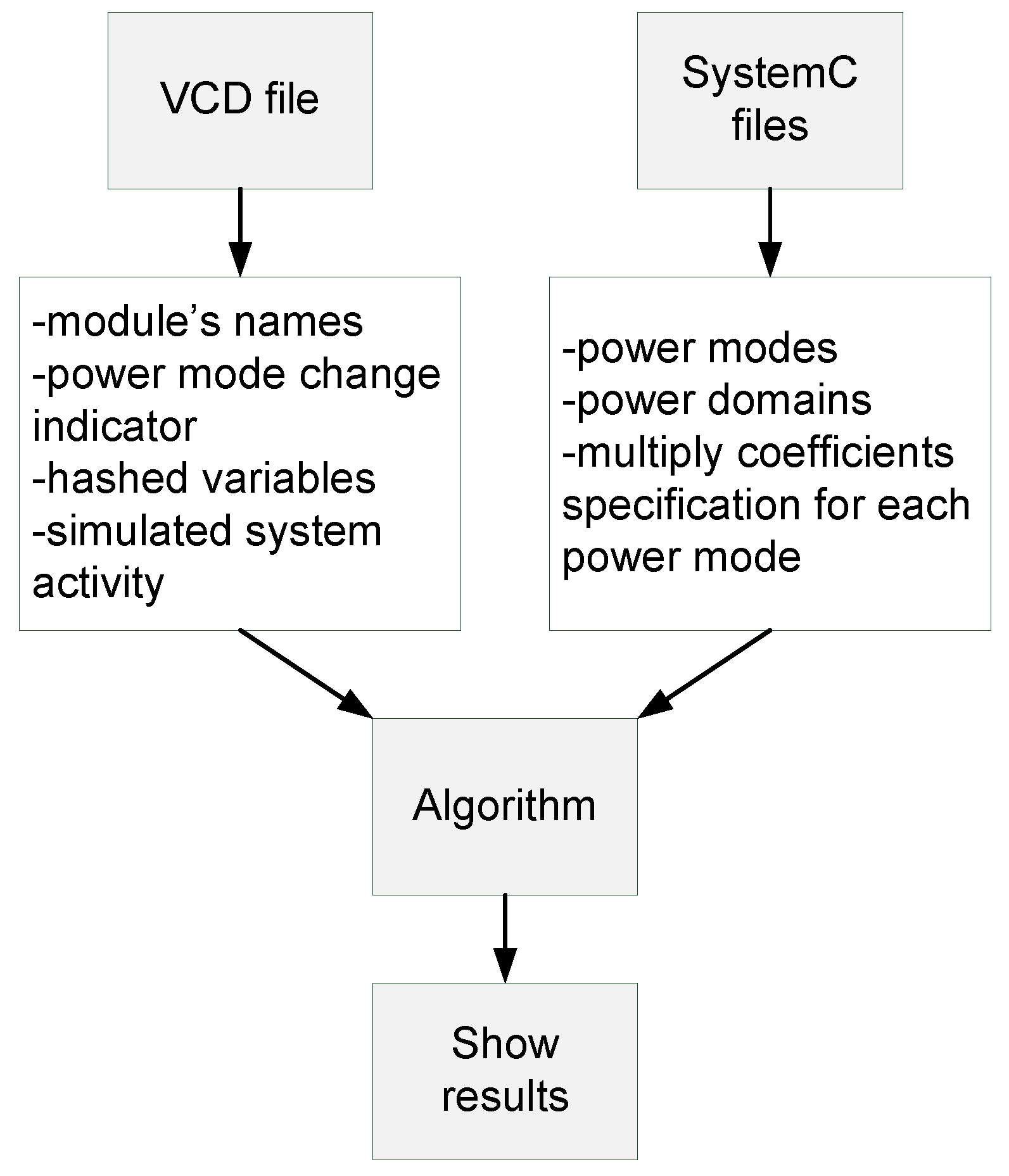
• First, we process data from SystemC (functional model description with power-management specification) and value change dump (VCD) system simulation data files.
• After processing the data, the algorithm begins to read the VCD file. Based on the simulation results, we then calculate the Hamming distance (i.e., the number of bits that switched their value in time).
• When the algorithm calculates the Hamming distance, it searches the SystemC processed data and find out the power state of a specific module.
• Based on the module state, the algorithm multiplies the calculated Hamming distance with the appropriate coefficient and adds the result to the overall energy consumption.
• The algorithm continues working this way until it reaches the end of the VCD file.

The requirements specified for the tool include the following: load and process SystemC and VCD files, enhanced Hamming-distance calculation for estimating energy consumption, present and export the results, simple control, and easy-to-read output.

3.1. Data Processing

Data processing from the VCD and SystemC files works in the following way: in the VCD file, the algorithm finds all modules, ports, and variables for each module. These variables are hashed into HashMap, in which the hash-key is represented by the variable and corresponding module names separated by a space (e.g., “dut cpu”). For each key, the previous state of the variable is saved to HashMap. In the SystemC file, the algorithm identifies a top module, which contains the power-management specification. The top module is identified based on the created hierarchy of SystemC modules. After identifying the top module, the algorithm starts to identify the power domains, power states, power modes, and the module constructor. The constructor contains the power management specification, especially in which power state a power domain operates in a specific power mode. This information is then saved. It is also necessary to calculate a coefficient for each DIFF_LEVEL power state, which is calculated as the arithmetic average between the NORMAL and DIFF_LEVEL power states.

3.2. Energy Estimation

After the initial data analysis and processing, the algorithm starts calculating the energy consumption. The algorithm begins by reading the VCD file. At first, it initializes the states of all variables, which are represented as a binary-vector value. The method initially looks at the power state and then calculates a summed Hamming distance of variable values for each SystemC module according to that power state. Based on the power state, the Hamming distance of a variable is either calculated or not. As previously stated, there are five types of power states, as defined in [38].

3.2.1. NORMAL

The component operating in this power state is supplied by the basic voltage of the system, and its working frequency is not modified. Therefore, the Hamming distance is calculated in the usual way, and the current variable state is saved as previous. For example, the previous variable state (binary vector) was 110011 and the current variable state is 100111. The Hamming distance between these two vectors is 2 (the number of bits that have changed). This value is added to the total sum, as expressed by

$$Total\_sum=Total\_sum+distance.$$

(3)

3.2.2. DIFF_LEVEL

In this power state, the component is operating at the voltage and/or frequency level, which is different from in the NORMAL power state. According to (1), both parameters influence dynamic power consumption. Therefore, the Hamming distance is multiplied by a coefficient representing the arithmetic average of the voltage and frequency ratios between the DIFF_LEVEL and NORMAL power states, and the current variable state is saved as previous. Such a modified distance is added to the total sum, as expressed by

$$c_{DIFF\_LEVEL}=\frac{1}{2}\times (\frac{V_{DIFF\_LEVEL}}{V_{NORMAL}}+\frac{f_{DIFF\_LEVEL}}{f_{NORMAL}})$$

(4)

$$Total\_sum=Total\_sum+distance\times c_{DIFF\_LEVEL}.$$

(5)

3.2.3. HOLD

This power state represents a stand-by state, in which the component remains powered, but its operation is stopped (i.e., operation frequency is 0). Because the internal state of the component should not change in this power state, the activity from VCD is ignored. Thus, the Hamming distance is not calculated and the previous variable state is not changed (i.e., the current variable state is ignored). The total sum is not incremented.

3.2.4. OFF

The component is powered-down in this power state. Because the component is not active in this state, the variable changes are ignored during the OFF state. However, the previous state is not retained; therefore, we use the 0-vector for calculating the Hamming distance. During entering of OFF power state, the distance is computed between the 0-vector and previous variable state. Then, the 0-vector is set as the previous variable state. Thus, during leaving the OFF power state, the distance is computed between the current variable state and 0-vector. These two computed Hamming distances are added to the total sum for the OFF period, as expressed by

$$Total\_sum+=distanc{e}_{enter\_OFF}+distanc{e}_{leave\_OFF}.$$

(6)

3.2.5. OFF_RET

In this power state, the component is powered down, but its internal state is retained. This means that the component is inactive in this power state. Thus, the algorithm does not compute the Hamming distance, similar to the HOLD power state. The result of this power state is that the total sum is not incremented.

After calculation of the total sum distance for each component, this distance is added to the overall system energy consumption, and it is also added to the consumption of the corresponding instance of a SystemC module.

In Figure 1, an overview of the novel power estimation method is illustrated, which also describes the inputs and outputs for each part of the method.

3.3. Energy-Estimation Tool

We have implemented the proposed method into an easy-to-use tool, mainly for evaluation purposes and to demonstrate its benefits. The tool works in the following way: after starting the tool, the SystemC and VCD files should be loaded. In the tool settings, the user can set where the output is to be saved and which output format should be used, and can change other parameters. After loading the files, the user starts automated processing of data from the input files, and subsequently initiates the calculation of energy consumption. The progress bar illustrates the progress of the calculation as a percentage, and the result is automatically exported in a format defined by the settings.

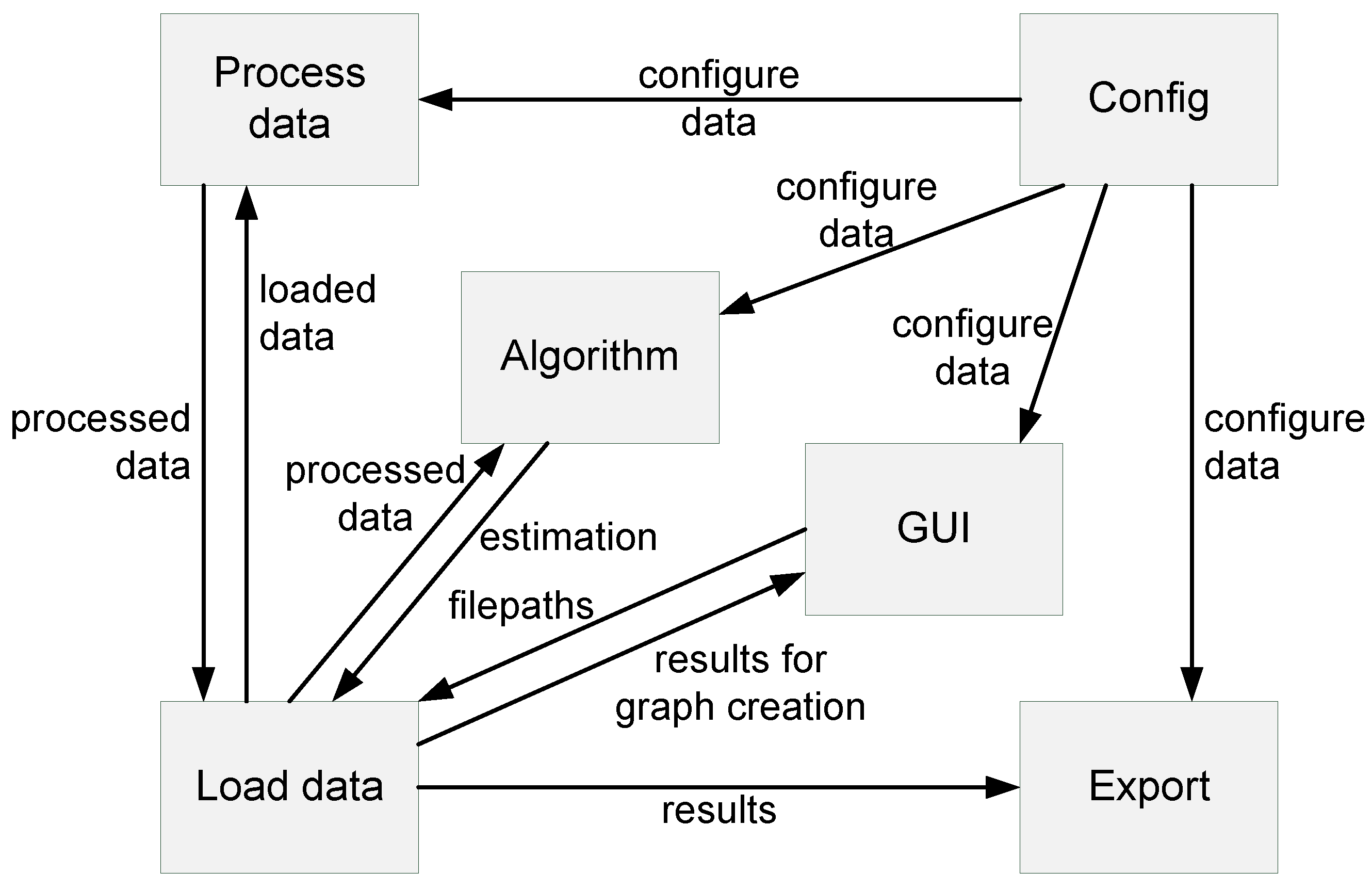
The tool is divided into six parts, and communication between these parts is shown in Figure 2. The tool is proposed in this way because of the modularity (i.e., a simple future extension of its functionality).

The Process data module serves for processing data from the VCD and SystemC files. Initially, this module accepts data from the Load data module. This module analyzes the data and sends the data back to Load data. At the start, the module accepts the configuration from the Config module.

The Config module serves for creating and saving the tool configuration. The configuration contains default values, but if a user changes the configuration in the tool settings, then the new configuration is saved. This module always sends the configuration data to each module at the start.

Load data is a simple module that serves for loading the data from the VCD and SystemC files. Another purpose of this module is storage. Initially, this module stores the loaded data, sends the data for processing, stores the analyzed data, sends the data to the Algorithm module, and stores the calculated power consumption (which is sent to the Export module).

The Export module serves for exporting the data into the XML, PDF, TXT, PNG formats, and for visualizing the data in the graphic user interface. The module exports the data based on either the accepted configuration or the current tool settings, which can be changed during runtime. By default, the results are exported to the graphic user interface.

The Algorithm module accepts the analyzed data. After accepting the analyzed data, the module starts calculating the consumed energy (according to the method described above) and then sends the result to the Load data module.

The GUI module is a graphic user interface. It serves for the user to control the tool and to see the results. In the GUI module, the user can load the SystemC and VCD files, which are processed. There is also a progress bar that displays the progress of the energy calculation. The GUI module also has the settings window.

Sending of data between modules is realized through interfaces. These load the data to a specific module, the data are then sent to another module after processing, and the data are deleted from the previous module.

A pseudo-algorithm that summarizes the proposed energy-estimation method is provided in Algorithm 1.

Algorithm 1: A pseudo-algorithm of the proposed method.
1 prepocessing SystemC file	21 end
2 foreach module do	22 preprocesing pairing variables
3 |  find topModule	23 foreach variable do
4 |  assing variables to module	24 |  pair systemC variables to VCD variables
5 end	25 end
6 findSpect (obj topModule){	26 power calculation
7   if(powerMangSpec)	27 set powerStateToEachModule
8     return moduleName;	28 foreach powerSimulationData do
9   else	29 |  if(changePowerState)
10     foreach module in topModule do	30 |    set powerStateToEachModule
11     |  findSpect(module)	31 |    calculate HammingDistance
12     end	32 |    addDistanceToSumResult
13   endif	33 |    addDistanceToModuleResult
14 }	34 |  else
15 preprocessing VCD file	35 |    calculate HammingDistance
16 foreach line do	36 |    addDistanceToSumResult
17 |  find variables	37 |    addDistanceToModuleResult
18 |  if(powerSimulationData)	38 |  endif
19 |    break;	39 end
20 |  endif	40 showAllResults

4. Experimental Results

To evaluate the accuracy of the proposed estimation method, we compared our results with those obtained using the Synopsys Power Compiler (using the NanGate_15nm_OCL technology library) from an equivalent very high-speed integrated circuits hardware description language (VHDL) model of the system. Such estimations are commonly used in industry. Because the proposed method produces a relative estimation (i.e., a sum of normalized Hamming distances of system variable values during the simulation), it cannot be directly compared to other methods that estimate the power in watts. Therefore, we compared the obtained ratios of estimated values for two design alternatives, using each of the two estimation methods.

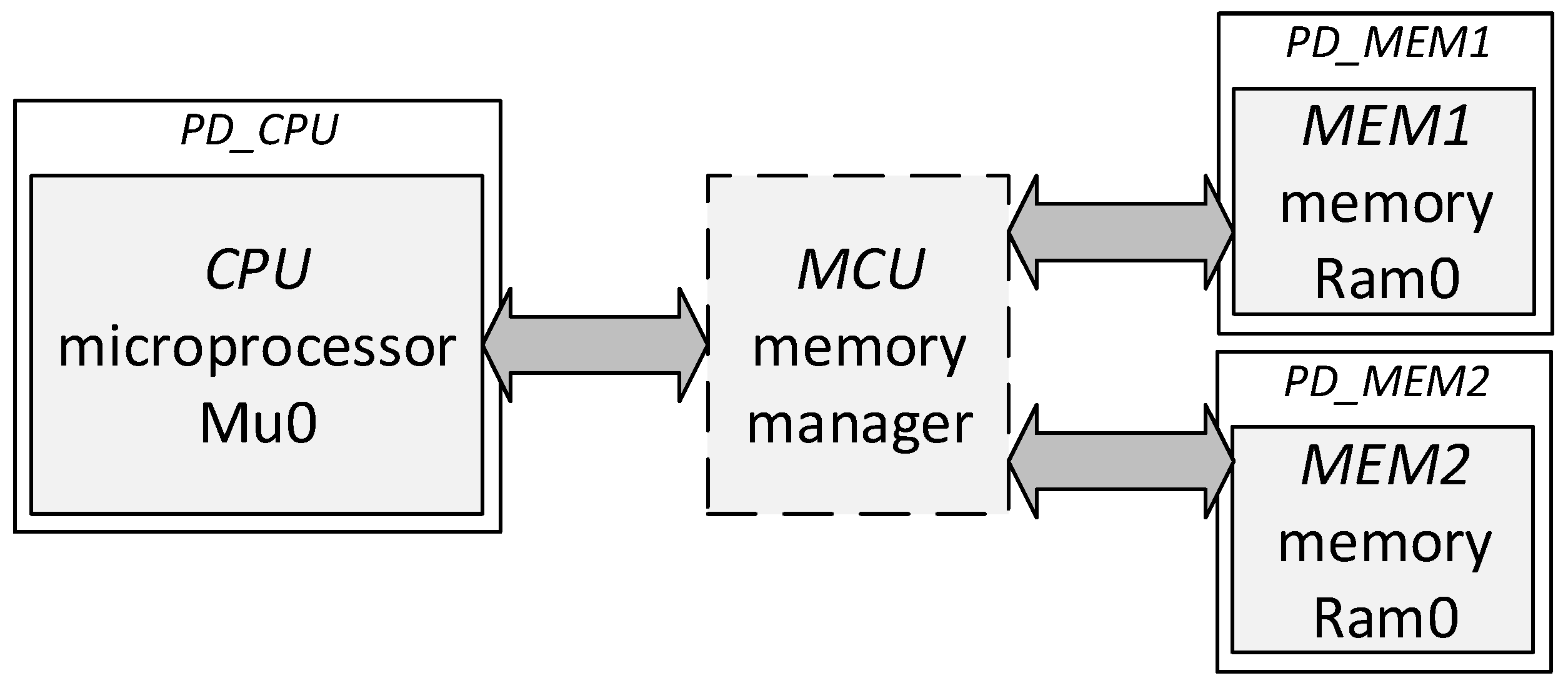
As a case study, we have used a simple system, consisting of one microprocessor (CPU) communicating with two memories (MEM1 and MEM2) via a memory manager (MCU). The CPU and MEM components are based on the mu0 and ram0 VHDL descriptions from [39]. MCU selects the MEM component, with which the CPU communicates. The abstract architecture of the case-study system is illustrated in Figure 3.

The experimental evaluation was more specifically processed in the following way: first, we described the same case-study system in both SystemC (system level) and VHDL (register-transfer level). We then created two alternatives in each model: with and without power management. At the system level, we used the PMS library for a specification of power management, whereas we used a power-intent specification in UPF at the register-transfer level.

As a next step, we estimated the power consumption of both VHDL alternatives (with and without the power management) using Power Compiler. Power Compiler reported the average switching power (i.e., the activity-dependent fraction of the tool’s power estimation) of the CPU component to $16.14\times {10}^{-4}$ mW for the alternative without power management, and $4.8\times {10}^{-4}$ mW for the alternative with power management. The computed ratio between the estimated values of these two alternatives is $\frac{6.14\times {10}^{-4}}{4.8\times {10}^{-4}}=1.28$. Similarly, we estimated the relative energy of both SystemC alternatives using the implemented PESL tool. The obtained results were 1,652,915 for the alternative without power management, and 1,569,213 for the alternative with the power management, which represents a ratio of approximately $1.0533$.

We then compared these two ratios (i.e., obtained by Power Compiler and by the PESL tool) by computing their relative percentage change. Using the example above, the change is computed as $\frac{1.0533-1.28}{1.28}\times 100\%=-17.71\%$. This means that the proposed method estimated the impact of power management on dynamic energy consumption with an inaccuracy of 17.71% when compared to the VHDL-based estimation produced by a professional tool.

Although the accuracy is not particularly high, we have improved the accuracy of the system-level estimation method. The original Hamming-distance computation method [19] does not consider a power-management effect; hence, it would always provide a ratio of 1. If we compare the inaccuracy of the original method and the inaccuracy of our method, we achieve an improvement of 4.16% with the proposed enhancement in this particular case. If we would prolong the simulation time when the device was inactive five times, we would achieve an improvement of approximately 30%. Since many of the IoT sensor-based devices can be inactive even 99% of their lifetime (due to the duty-cycle communication restriction in long-range IoT networks [40]), the original method not considering power management can be totally inaccurate, making an improvement of hundreds of percent.

To indicate the key benefit of the proposed enhancement clearly, we provide an experiment illustrating system-level power-management exploration using the proposed method. Using SystemC/PMS, we specified four alternative power-management architectures for the previously mentioned case-study system, in which each component had a dedicated power domain called PD_<component name> (see Figure 3). We then estimated the effect on its dynamic energy consumption (during the same simulation). The results are provided in

Table 1. Illustration of the power-management exploration.

Power Management	Power Mode	Power States in Power Domains			Estimated Dynamic	Comparison
Alternative		PD_CPU	PD_MEM1	PD_MEM2	Energy
A	PM1	NORMAL	NORMAL	NORMAL	10,919,512	100%
	PM2	NORMAL	NORMAL	NORMAL
	PM3	NORMAL	NORMAL	NORMAL
	PM4	NORMAL	NORMAL	NORMAL
B	PM1	NORMAL	NORMAL	NORMAL	7,956,291	72.9%
	PM2	NORMAL	NORMAL	OFF_RET
	PM3	NORMAL	HOLD	NORMAL
	PM4	OFF	HOLD	OFF_RET
C	PM1	NORMAL	NORMAL	NORMAL	7,956,290	72.9%
	PM2	NORMAL	NORMAL	HOLD
	PM3	NORMAL	HOLD	NORMAL
	PM4	HOLD	HOLD	HOLD
D	PM1	NORMAL	NORMAL	NORMAL	8,072,960	73.9%
	PM2	NORMAL	NORMAL	HOLD
	PM3	NORMAL	HOLD	NORMAL
	PM4	NORMAL	HOLD	HOLD
E	PM1	NORMAL	NORMAL	NORMAL	9,486,080	86.9%
	PM2	NORMAL	NORMAL	HOLD
	PM3	NORMAL	NORMAL	NORMAL
	PM4	OFF	OFF	OFF

. In the table, the alternative A is the specification without the power management, and the other alternatives include the specifications of various combinations of power states in the system power modes (i.e., various power architectures). The second column from the right contains the estimated dynamic energy of the system under the specified power management in the number of bit-flips during the simulation, adjusted according to the proposed method in Section 3.2. The final column presents a comparison of the estimated dynamic energy for the power-management alternatives and the alternative A (i.e., without the power-management specification). The formula used to obtain the values in the Comparison column is $\frac{EDE\left(X\right)}{EDE\left(A\right)}\times 100\%$, where EDE is the estimated dynamic energy value from the corresponding column, X is the alternative from the first column, and A is the alternative A.

According to the results, the alternatives B and C are the most energy-efficient. We obtained the same estimations for these alternatives because the OFF/OFF_RET power states in the alternative B were substituted by the HOLD power state in the alternative C. Further, according to the proposed method, all of them have the same effect on the dynamic energy. The alternative D has a slightly higher estimated energy consumption, because the CPU is active during the whole simulation. Similarly, the alternative E has even higher energy consumption, because the MEM2 is active even when not being used by the CPU (i.e., while it is communicating with the MEM1). We have proved through this experiment that the proposed method can be used for system-level power-management exploration. This would not be possible using the original Hamming-distance computation method [19], because it would return the same result for each alternative. Moreover, we did not need to re-simulate the design in this experiment, because we have not modified power-mode switching in the alternatives (i.e., the power modes were switched in the same simulation time in each alternative). This would not be possible in any other existing power-management exploration method. Thus, the proposed method enables faster power-management exploration than the existing methods. This improvement was by a factor of several magnitudes (i.e., seconds instead of hours).

Discussion

As previously mentioned, no other existing similar tool (i.e., taking power management into account while estimating the dynamic power) is freely available; hence, we could not experimentally compare the solutions. However, we at least tried to compare our solution to the TLM Power 3 tool [22] (in addition to the original Hamming-distance computation method [19]) based on an analysis, and present a summary of the differences in

Table 2. Comparisons.

Solution	Top-Down Design	Accuracy	Estimation	Required Knowledge
TLM Power 3	No	High	Real Units	High
Ref. [19]	Yes	Low	Relative Units	Low
PESL	Yes	Medium	Relative Units	Low

.

It can be observed that our solution has several advantages. Using PESL, we can realize a pure top-down design approach. This is not possible using the TLM Power 3 tool, because it relies on data from previous implementations of system components. PESL is very intuitive and easy-to-use, while the TLM Power 3 tool is more complex and knowledge is required to set it correctly. Another advantage lies in the estimation time. We can estimate the effect of an alternative power-management specification without starting a new simulation. However, modifications in system specification that do not require a new simulation must keep the number of power modes and their switching time intact. With such a PESL feature, we can easily try many power-management alternatives. In comparison, TLM Power 3 would need to run a new simulation every time. We can express this speed advantage by the following equations.

Time of power estimation using TLM Power 3 can be expressed by

$$t_{pc}=n\times (t_s+t_e),$$

(7)

where $t_{pc}$ is power-calculation time, n is the number of alternatives, $t_s$ is the simulation time, and $t_e$ is power-estimation time. Time of power estimation using PESL can be expressed by

$$t_{pc}=m\times t_s+n\times t_e,$$

(8)

where m is the number of required simulations ($m\le n$).

There are some disadvantages with PESL. For example, it can only provide a relative power estimation, whereas TLM Power 3 provides estimations in real units. Further, PESL is less accurate than TLM Power 3. However, it is better than in the case of [19], which could not be used for power-management exploration of the same system. Moreover, the accuracy of the PESL estimation is good enough to provide a difference in the power estimation of various power-management architectures.

Compared to lower-level power estimations (e.g., at the register–transfer level, gate level, or post placement and route stage), the proposed method is less accurate due to higher abstraction, but is significantly faster. Lower design-abstraction levels include more details; thus, more information can be used during the estimation. However, the simulation takes longer with a more-detailed model.

5. Conclusions

In this paper, we proposed a novel method for system-level energy estimation that considers the power-management effect. We also described the implementation of this method in a user-friendly tool. By analyzing the SystemC and VCD files, this method calculates the dynamic energy consumption using enhanced Hamming-distance computation. Using the computed relative energy consumption, a designer can efficiently compare two design alternatives of the same power-managed system and select the most appropriate. The results can be exported into various file formats (XML, PDF, TXT or PNG) for simplified further processing by another tool.

The proposed method is especially suitable for fast power-management exploration at a system level. The reason for this is that the method does not require re-simulation of the system model after the power management is modified, if the number of power modes and their switching has not changed. Thus, a designer is able to “try” multiple power-state variations or partitioning of the system into the power domains in a very short time without re-simulation. This is a unique approach that has never been seen before.

We expect that the proposed method will be faster, simpler, and more accurate compared to other system-level power-estimation methods usable for top-down design, because it considers the power states of each module during the simulation at a system level. The experimental results demonstrated that the novel method estimated lower energy consumption when it should be lower (according to the specified power management), whereas the original method would have estimated the same energy as in the system without power management. Thus, the proposed method improved the accuracy compared to the original Hamming-distance calculation method.