Upsampling Real-Time, Low-Resolution CCTV Videos Using Generative Adversarial Networks


Abstract
:1. Introduction
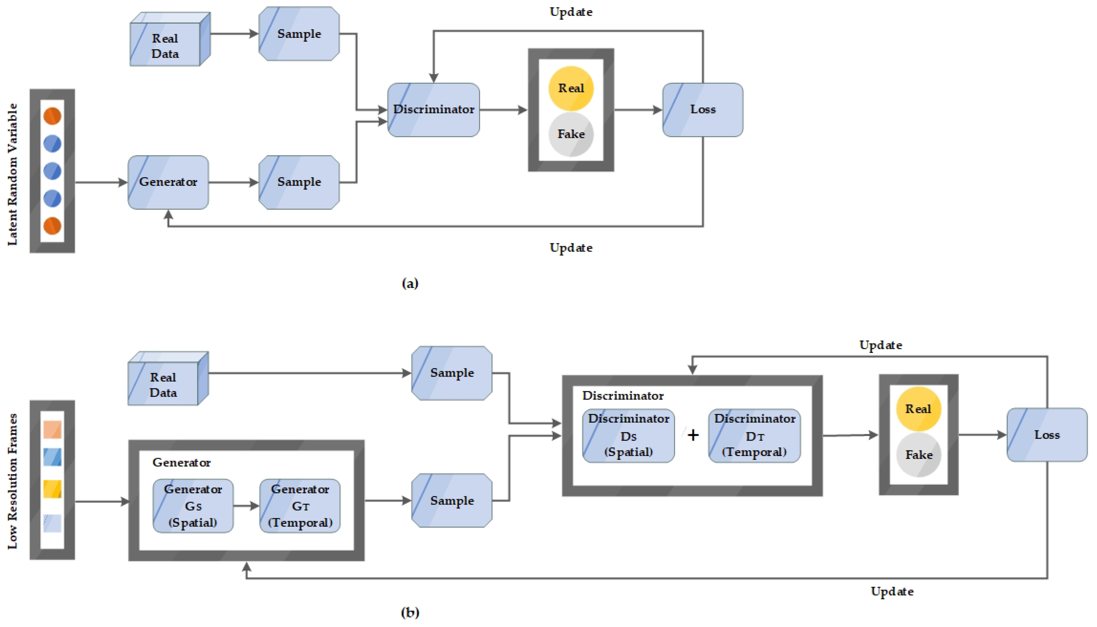
- Dual spatio-temporal generators and discriminators to enhance the low-resolution CCTV videos with high accuracy.
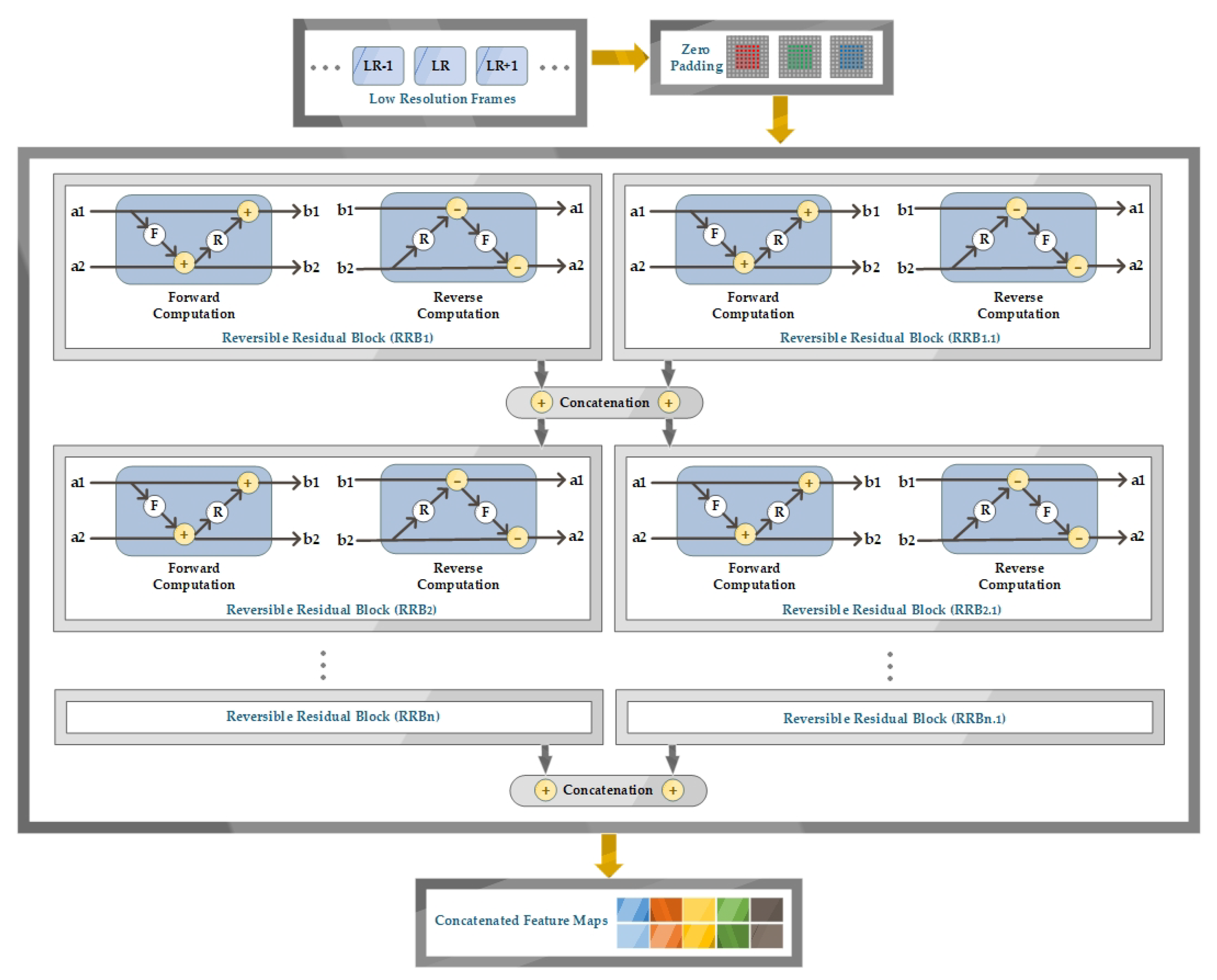
- Concatenated reversible residual blocks in generators which help in distinguishing between low and high-resolution frames and extract intricate features without information loss.
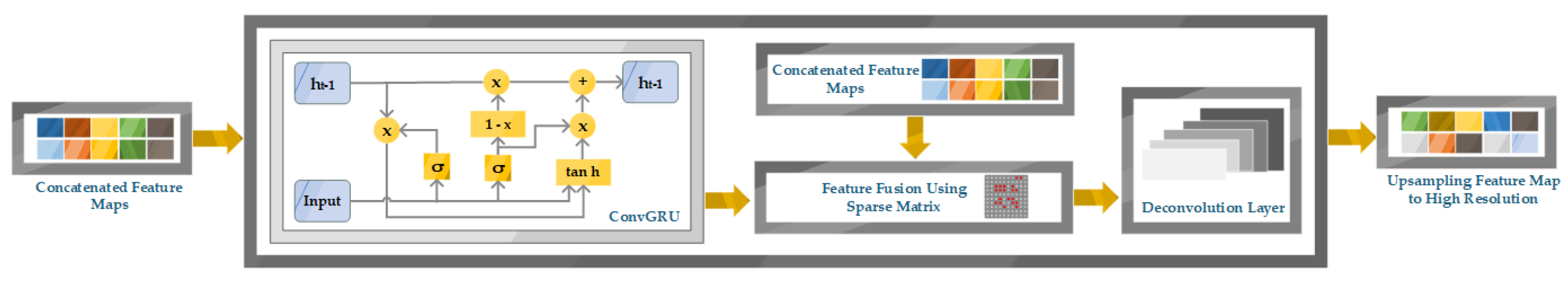
- Mapping between low and high-resolution frames in an adaptive way by using a sparse matrix for fused features.
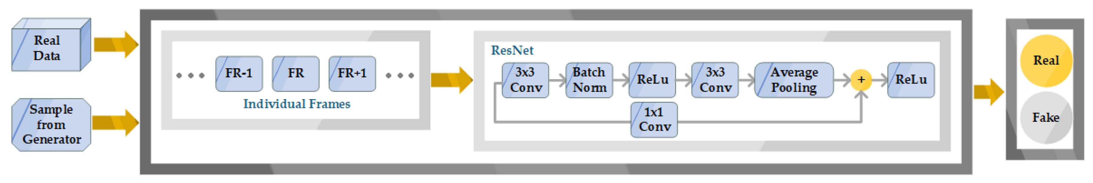
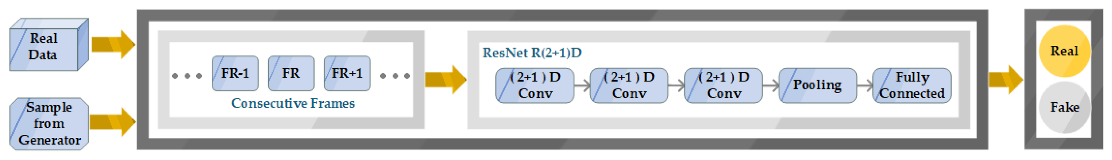
- Discriminators with R(2 + 1)D convolutional ResNet for better optimization and performance.
2. Related Works
3. Data
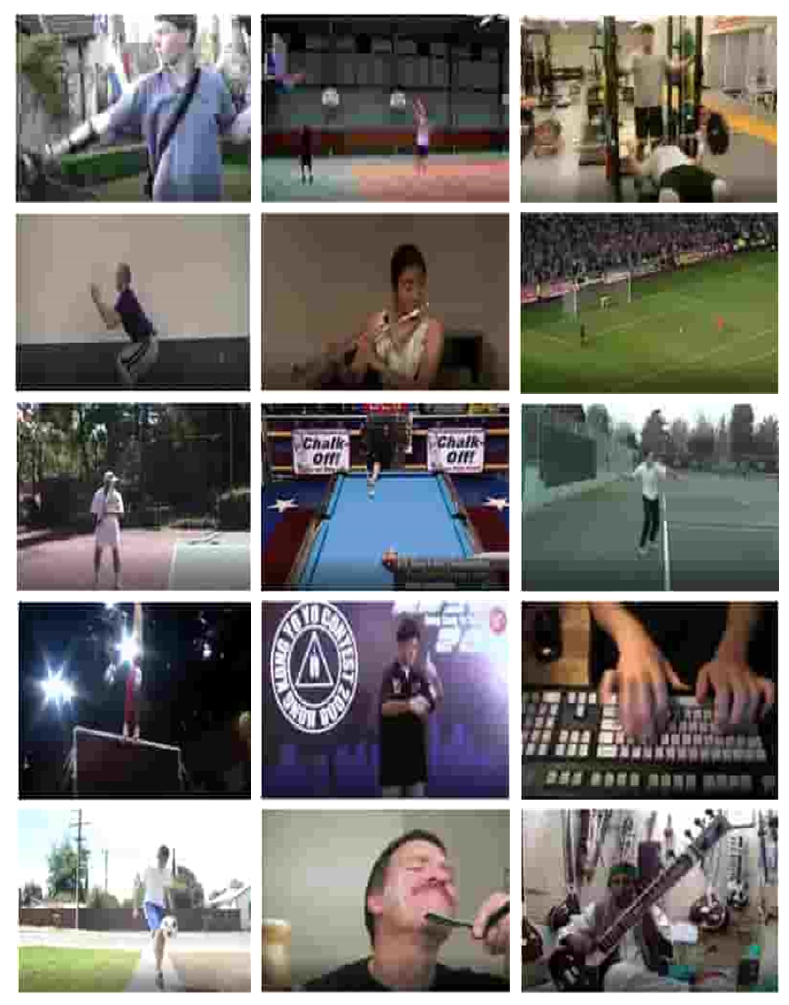
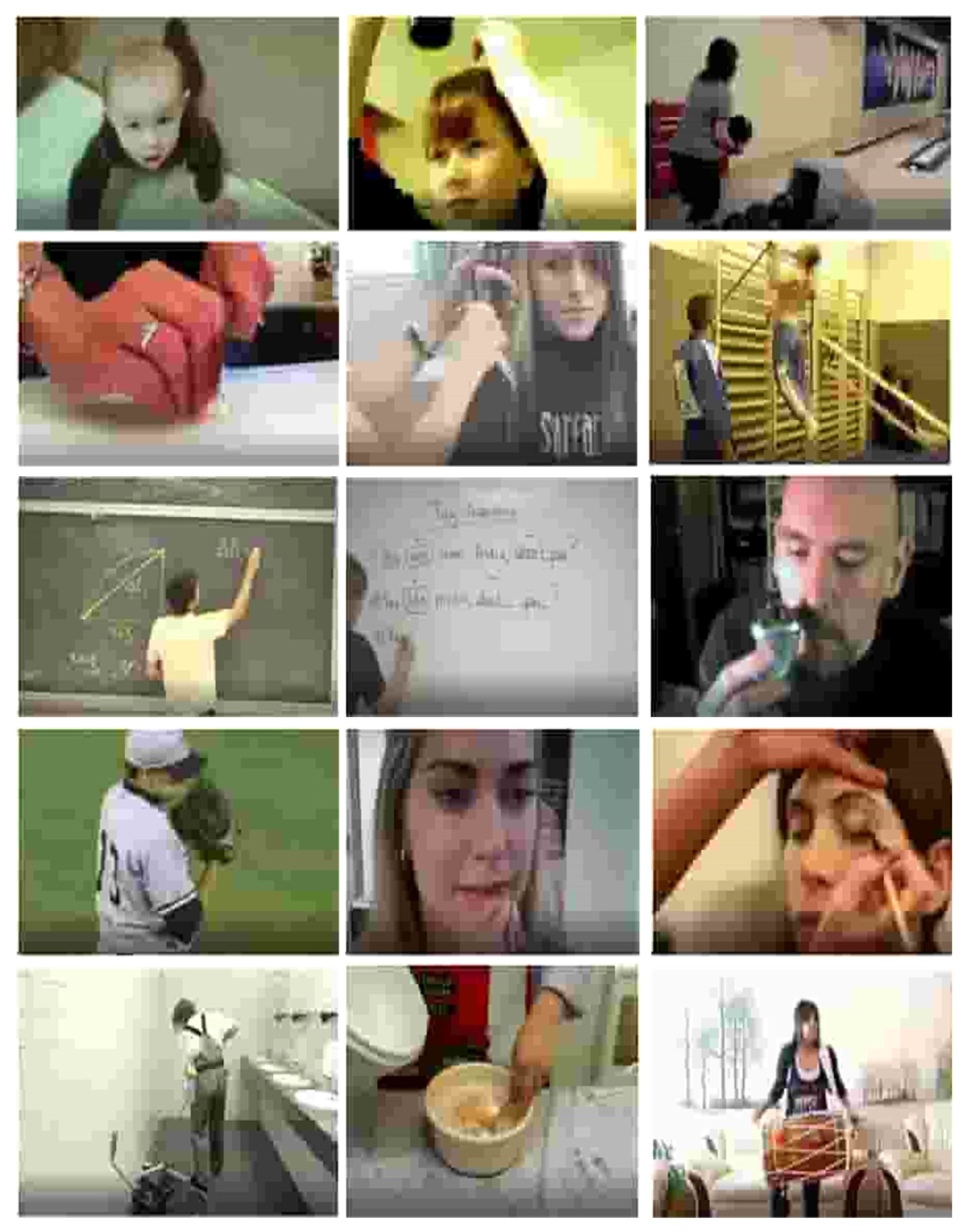
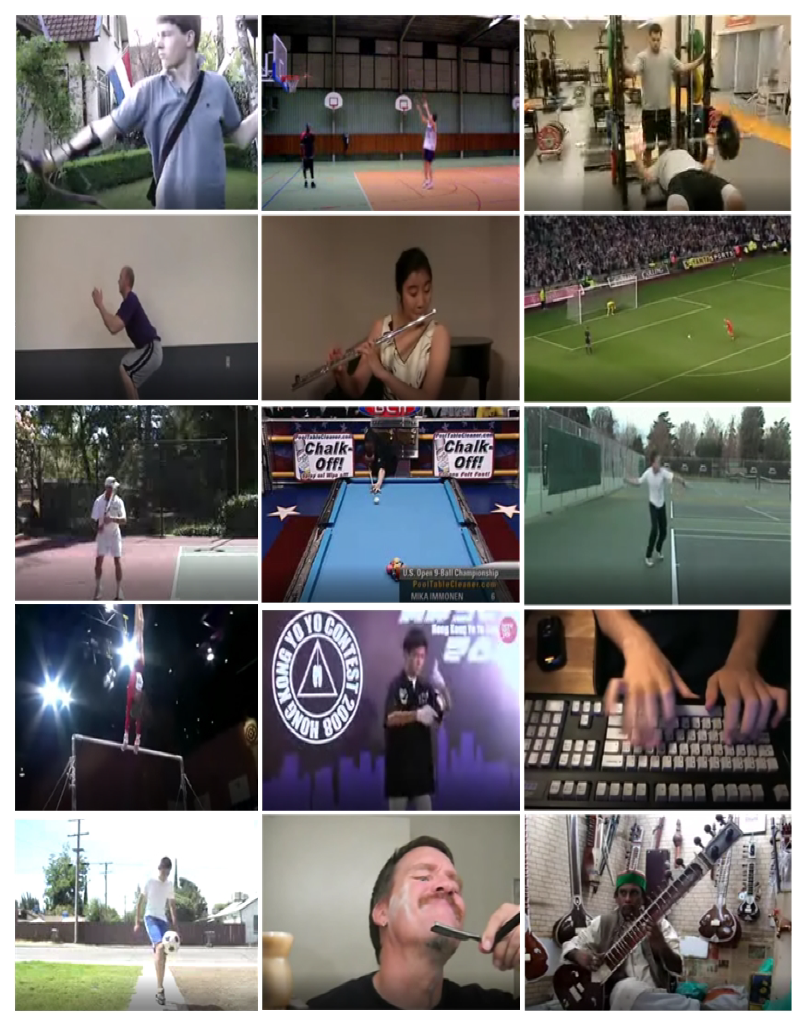
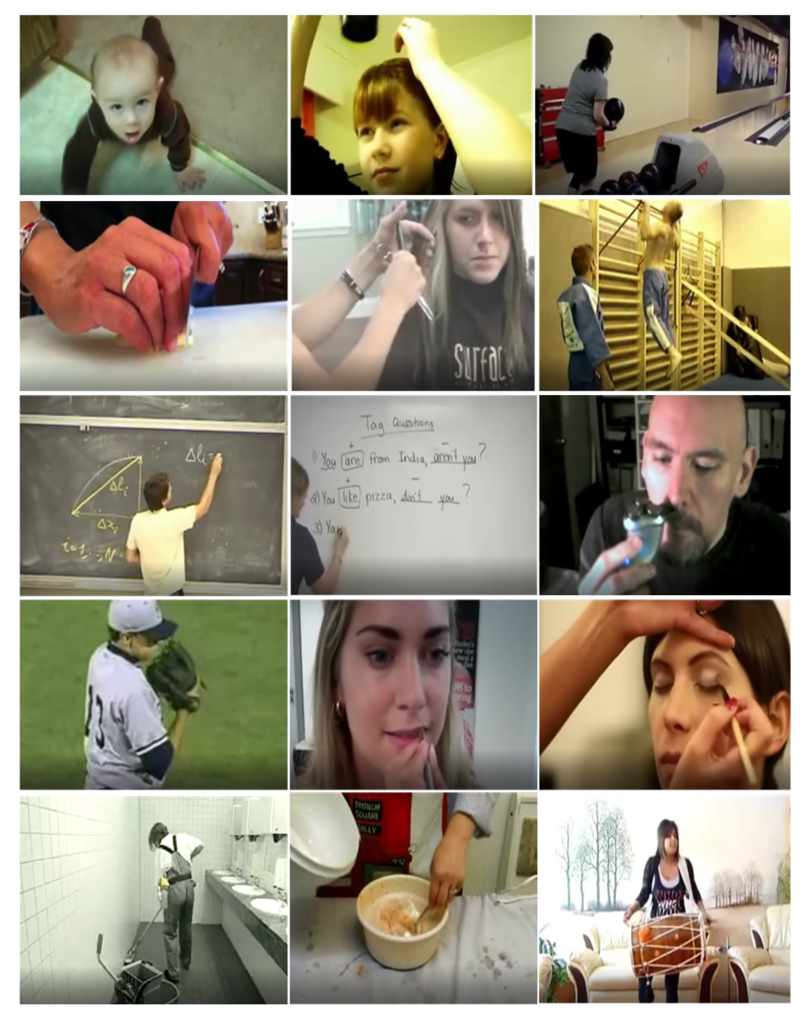
3.1. Kinetics-700
3.2. UCF101
3.3. HMDB51
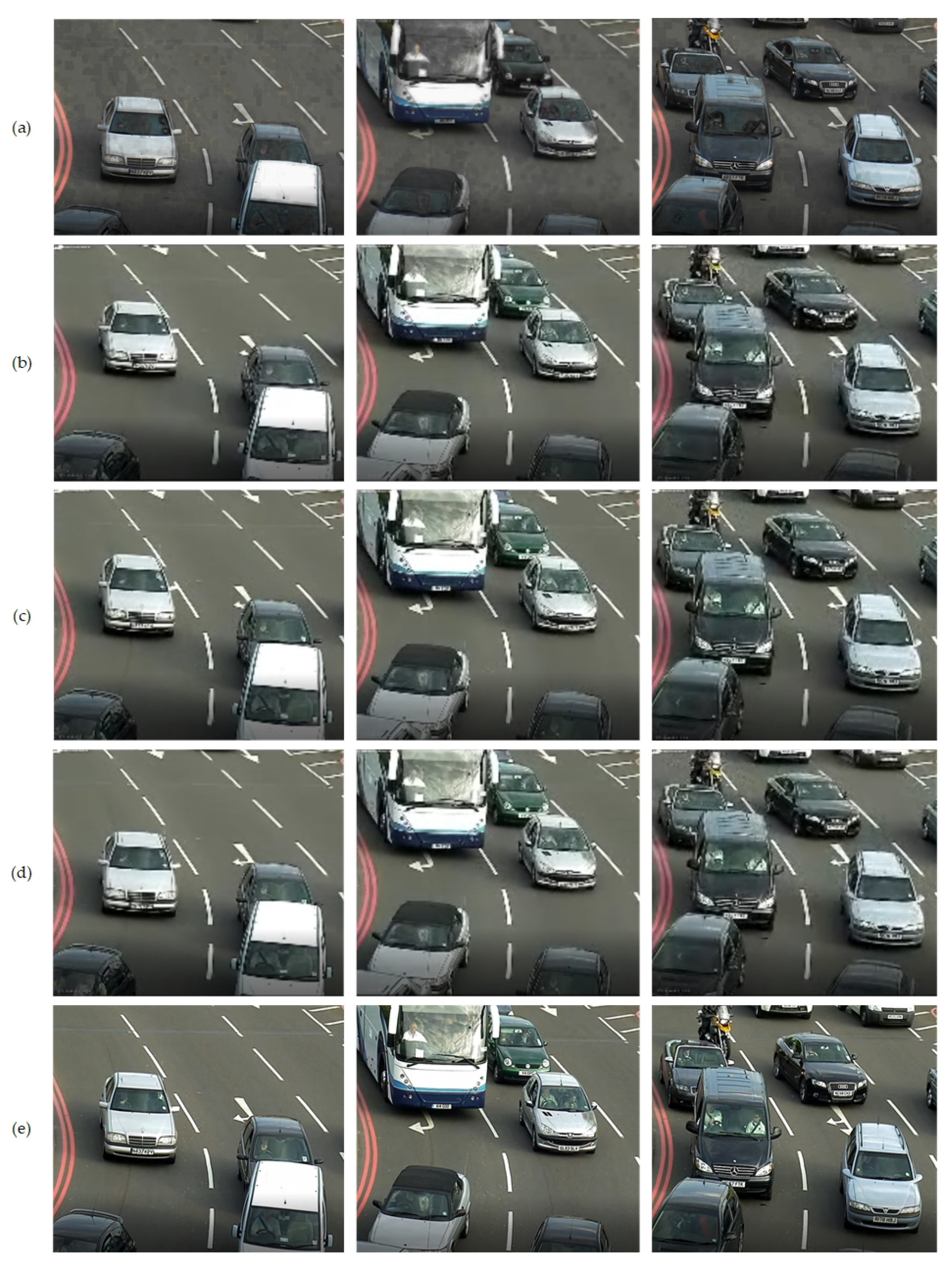
3.4. IITH_Helmet2
4. Proposed Generative Adversarial Networks for Upsampling Real-Time Low-Resolution CCTV Videos
4.1. Overview
4.2. Spatial Generator
4.3. Temporal Generator
4.4. Spatial Discriminator
4.5. Temporal Discriminator
5. Environment and Training
5.1. Experimental Setup
5.2. Training
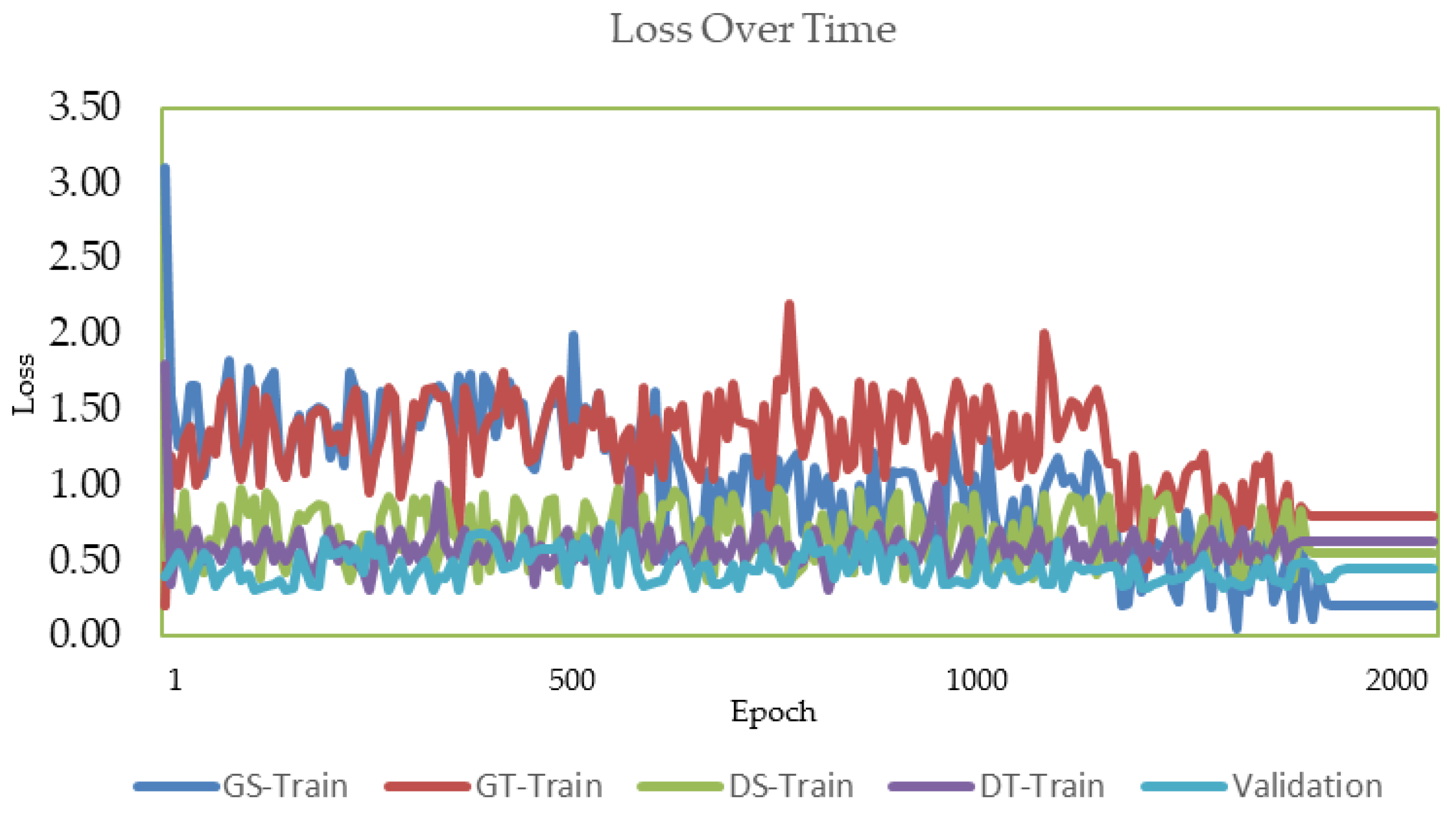
5.3. Loss Functions
5.3.1. Content Loss
5.3.2. Adversarial Loss
5.3.3. Perceptual Loss
6. Evaluation
7. Conclusions
Author Contributions
Funding
Conflicts of Interest
References
- Ashby, M.P. The value of CCTV surveillance cameras as an investigative tool: An empirical analysis. Eur. J. Crim. Policy Res. 2017, 23, 441–459. [Google Scholar] [CrossRef] [Green Version]
- International Trends in Video Surveillancepublic Transport Gets Smarter. Available online: https://www.uitp.org/sites/default/files/cck-focus-papers-files/1809-Statistics%20Brief%20-%20Videosurveillance-Final.pdf (accessed on 15 July 2020).
- Size of the Global Video Surveillance Market between 2016 and 2025. Available online: https://www.statista.com/statistics/864838/video-surveillance-market-size-worldwide/ (accessed on 15 July 2020).
- Khan, P.W.; Byun, Y. A Blockchain-Based Secure Image Encryption Scheme for the Industrial Internet of Things. Entropy 2020, 22, 175. [Google Scholar] [CrossRef] [Green Version]
- Park, N.; Kim, B.G.; Kim, J. A Mechanism of Masking Identification Information regarding Moving Objects Recorded on Visual Surveillance Systems by Differentially Implementing Access Permission. Electronics 2019, 8, 735. [Google Scholar] [CrossRef] [Green Version]
- Khan, P.W.; Xu, G.; Latif, M.A.; Abbas, K.; Yasin, A. UAV’s agricultural image segmentation predicated by clifford geometric algebra. IEEE Access 2019, 7, 38442–38450. [Google Scholar] [CrossRef]
- Clark, A.; Donahue, J.; Simonyan, K. Efficient video generation on complex datasets. arXiv 2019, arXiv:1907.06571. [Google Scholar]
- Khan, P.W.; Byun, Y.C.; Park, N. A Data Verification System for CCTV Surveillance Cameras Using Blockchain Technology in Smart Cities. Electronics 2020, 9, 484. [Google Scholar] [CrossRef] [Green Version]
- Yang, W.; Feng, J.; Xie, G.; Liu, J.; Guo, Z.; Yan, S. Video super-resolution based on spatial-temporal recurrent residual networks. Comput. Vis. Image Underst. 2018, 168, 79–92. [Google Scholar] [CrossRef]
- Ballas, N.; Yao, L.; Pal, C.; Courville, A. Delving deeper into convolutional networks for learning video representations. arXiv 2015, arXiv:1511.06432. [Google Scholar]
- Tran, D.; Wang, H.; Torresani, L.; Ray, J.; LeCun, Y.; Paluri, M. A closer look at spatiotemporal convolutions for action recognition. In Proceedings of the IEEE Conference on Computer Vision and Pattern Recognition, Salt Lake City, UT, USA, 18–22 June 2018; pp. 6450–6459. [Google Scholar]
- Tulyakov, S.; Liu, M.Y.; Yang, X.; Kautz, J. Mocogan: Decomposing motion and content for video generation. In Proceedings of the IEEE Conference on Computer Vision and Pattern Recognition, Salt Lake City, UT, USA, 18–22 June 2018; pp. 1526–1535. [Google Scholar]
- Saito, M.; Saito, S.; Koyama, M.; Kobayashi, S. Train Sparsely, Generate Densely: Memory-Efficient Unsupervised Training of High-Resolution Temporal GAN. Int. J. Comput. Vis. 2020. [Google Scholar] [CrossRef]
- Saito, M.; Matsumoto, E.; Saito, S. Temporal generative adversarial nets with singular value clipping. In Proceedings of the IEEE International Conference on Computer Vision, Venice, Italy, 22–29 October 2017; pp. 2830–2839. [Google Scholar]
- Brock, A.; Donahue, J.; Simonyan, K. Large scale gan training for high fidelity natural image synthesis. arXiv 2018, arXiv:1809.11096. [Google Scholar]
- Gomez, A.N.; Ren, M.; Urtasun, R.; Grosse, R.B. The reversible residual network: Backpropagation without storing activations. In Advances in Neural Information Processing Systems; MIT Press: Cambridge, MA, USA, 2017; pp. 2214–2224. [Google Scholar]
- Zhu, X.; Li, Z.; Zhang, X.Y.; Li, C.; Liu, Y.; Xue, Z. Residual invertible spatio-temporal network for video super-resolution. In Proceedings of the AAAI Conference on Artificial Intelligence, Honolulu, HI, USA, 27 January–1 February 2019; Volume 33, pp. 5981–5988. [Google Scholar]
- Samaniego, E.; Anitescu, C.; Goswami, S.; Nguyen-Thanh, V.M.; Guo, H.; Hamdia, K.; Zhuang, X.; Rabczuk, T. An energy approach to the solution of partial differential equations in computational mechanics via machine learning: Concepts, implementation and applications. Comput. Methods Appl. Mech. Eng. 2020, 362, 112790. [Google Scholar] [CrossRef] [Green Version]
- Guo, H.; Zhuang, X.; Rabczuk, T. A deep collocation method for the bending analysis of Kirchhoff plate. Comput. Mater Contin. 2019, 59, 433–456. [Google Scholar] [CrossRef]
- Vondrick, C.; Pirsiavash, H.; Torralba, A. Generating videos with scene dynamics. In Advances in Neural Information Processing Systems; MIT Press: Cambridge, MA, USA, 2016; pp. 613–621. [Google Scholar]
- Dong, C.; Loy, C.C.; He, K.; Tang, X. Image super-resolution using deep convolutional networks. IEEE Trans. Pattern Anal. Mach. Intell. 2015, 38, 295–307. [Google Scholar] [CrossRef] [PubMed] [Green Version]
- Kim, J.; Kwon Lee, J.; Mu Lee, K. Accurate image super-resolution using very deep convolutional networks. In Proceedings of the IEEE Conference on Computer Vision and Pattern Recognition, Las Vegas, NV, USA, 27–30 June 2016; pp. 1646–1654. [Google Scholar]
- Ledig, C.; Theis, L.; Huszár, F.; Caballero, J.; Cunningham, A.; Acosta, A.; Aitken, A.; Tejani, A.; Totz, J.; Wang, Z.; et al. Photo-realistic single image super-resolution using a generative adversarial network. In Proceedings of the IEEE Conference on Computer Vision and Pattern Recognition, Honolulu, HI, USA, 21–26 July 2017; pp. 4681–4690. [Google Scholar]
- Lai, W.S.; Huang, J.B.; Ahuja, N.; Yang, M.H. Deep laplacian pyramid networks for fast and accurate super-resolution. In Proceedings of the IEEE Conference on Computer Vision and Pattern Recognition, Honolulu, HI, USA, 21–26 July 2017; pp. 624–632. [Google Scholar]
- Tai, Y.; Yang, J.; Liu, X. Image super-resolution via deep recursive residual network. In Proceedings of the IEEE Conference on Computer Vision and Pattern Recognition, Honolulu, HI, USA, 21–26 July 2017; pp. 3147–3155. [Google Scholar]
- Johnson, J.; Alahi, A.; Fei-Fei, L. Perceptual losses for real-time style transfer and super-resolution. In European Conference on Computer Vision; Springer: Cham, Switzerland, 2016; pp. 694–711. [Google Scholar]
- Goodfellow, I.; Pouget-Abadie, J.; Mirza, M.; Xu, B.; Warde-Farley, D.; Ozair, S.; Courville, A.; Bengio, Y. Generative adversarial nets. In Advances in Neural Information Processing Systems; MIT Press: Cambridge, MA, USA, 2014; pp. 2672–2680. [Google Scholar]
- Sajjadi, M.S.; Scholkopf, B.; EnhanceNet, M.H. Single Image Super-Resolution through Automated Texture Synthesis. Max-Planck-Inst. Intell. Syst. Spemanstr 2016, 23, 4501–4510. [Google Scholar]
- Lim, B.; Son, S.; Kim, H.; Nah, S.; Mu Lee, K. Enhanced deep residual networks for single image super-resolution. In Proceedings of the IEEE Conference on Computer Vision and Pattern Recognition Workshops, Honolulu, HI, USA, 22–25 July 2017; pp. 136–144. [Google Scholar]
- Wang, X.; Yu, K.; Wu, S.; Gu, J.; Liu, Y.; Dong, C.; Qiao, Y.; Change Loy, C. Esrgan: Enhanced super-resolution generative adversarial networks. In Proceedings of the European Conference on Computer Vision (ECCV), Munich, Germany, 8–14 September 2018. [Google Scholar]
- Carreira, J.; Noland, E.; Hillier, C.; Zisserman, A. A short note on the kinetics-700 human action dataset. arXiv 2019, arXiv:1907.06987. [Google Scholar]
- Soomro, K.; Zamir, A.R.; Shah, M. UCF101: A dataset of 101 human actions classes from videos in the wild. arXiv 2012, arXiv:1212.0402. [Google Scholar]
- Kuehne, H.; Jhuang, H.; Garrote, E.; Poggio, T.; Serre, T. HMDB: A large video database for human motion recognition. In Proceedings of the 2011 International Conference on Computer Vision, Barcelona, Spain, 6–13 November 2011; pp. 2556–2563. [Google Scholar]
- Vishnu, C.; Singh, D.; Mohan, C.K.; Babu, S. Detection of motorcyclists without helmet in videos using convolutional neural network. In Proceedings of the 2017 International Joint Conference on Neural Networks, (IJCNN), Anchorage, AK, USA, 14–19 May 2017; pp. 3036–3041. [Google Scholar] [CrossRef]
- Dinh, L.; Krueger, D.; Bengio, Y. Nice: Non-linear independent components estimation. arXiv 2014, arXiv:1410.8516. [Google Scholar]
- Dinh, L.; Sohl-Dickstein, J.; Bengio, S. Density estimation using real nvp. arXiv 2016, arXiv:1605.08803. [Google Scholar]
- Jiang, Y.; Li, J. Generative Adversarial Network for Image Super-Resolution Combining Texture Loss. Appl. Sci. 2020, 10, 1729. [Google Scholar] [CrossRef] [Green Version]
- Simonyan, K.; Zisserman, A. Very deep convolutional networks for large-scale image recognition. arXiv 2014, arXiv:1409.1556. [Google Scholar]
- Webster, R.; Rabin, J.; Simon, L.; Jurie, F. Detecting overfitting of deep generative networks via latent recovery. In Proceedings of the IEEE Conference on Computer Vision and Pattern Recognition, Long Beach, CA, USA, 15–21 June 2019; pp. 11273–11282. [Google Scholar]


| Components | Specifications and Versions |
|---|---|
| Operating System | Ubuntu 18.04.3 LTS |
| Memory | 32 GB |
| GPU | Nvidia GeForce GTX 1060 3 GB |
| API | Tensorflow 1.x |
| Interface | CUDA Toolkit version 10.1.243 and cuDNN version 7.6.5 |
| CPU | Intel(R) Core(TM) i7-8700 CPU @ 3.20 GHz |
| Language | Python 3.6.5 |
| Model | Resolution | IS | FID | PSNR | SSIM | CT-Per Frame (msec) |
|---|---|---|---|---|---|---|
| DVD-GAN | 512p | 27.24 ± 0.32 | 44.35 ± 0.45 | 23.26 | 83.90 | 750 |
| 720p | 29.71 ± 0.76 | 43.77 ± 0.53 | 23.47 | 80.12 | 800 | |
| 960p | 24.32 ± 0.78 | 46.38 ± 0.21 | 24.35 | 81.34 | 900 | |
| BigGAN | 512p | 34.66 ± 0.74 | 38.57 ± 0.32 | 27.89 | 85.56 | 700 |
| 720p | 33.92 ± 0.25 | 38.22 ± 0.74 | 27.63 | 86.73 | 750 | |
| 960p | 35.43 ± 0.66 | 35.84 ± 0.45 | 28.93 | 86.98 | 800 | |
| BigGAN-deep | 512p | 33.45 ± 0.48 | 29.99 ± 0.74 | 31.32 | 89.99 | 700 |
| 720p | 33.69 ± 0.44 | 28.43 ± 0.87 | 32.75 | 89.92 | 780 | |
| 960p | 36.43 ± 0.88 | 27.65 ± 0.35 | 32.66 | 90.12 | 850 | |
| Proposed GAN | 512p | 48.44 ± 0.36 | 17.43 ± 0.63 | 40.12 | 93.45 | 500 |
| 720p | 49.65 ± 0.83 | 16.94 ± 0.39 | 41.32 | 93.98 | 650 | |
| 960p | 49.99 ± 0.64 | 16.92 ± 0.55 | 41.59 | 94.25 | 700 |
© 2020 by the authors. Licensee MDPI, Basel, Switzerland. This article is an open access article distributed under the terms and conditions of the Creative Commons Attribution (CC BY) license (http://creativecommons.org/licenses/by/4.0/).
Share and Cite
Hazra, D.; Byun, Y.-C. Upsampling Real-Time, Low-Resolution CCTV Videos Using Generative Adversarial Networks. Electronics 2020, 9, 1312. https://doi.org/10.3390/electronics9081312
Hazra D, Byun Y-C. Upsampling Real-Time, Low-Resolution CCTV Videos Using Generative Adversarial Networks. Electronics. 2020; 9(8):1312. https://doi.org/10.3390/electronics9081312
Chicago/Turabian StyleHazra, Debapriya, and Yung-Cheol Byun. 2020. "Upsampling Real-Time, Low-Resolution CCTV Videos Using Generative Adversarial Networks" Electronics 9, no. 8: 1312. https://doi.org/10.3390/electronics9081312