1. Introduction
Recently, the fifth-generation (5G) wireless communication system, known as new radio (NR), has been successfully commercialized globally. With the development of 5G NR, the performance and functionality of cellular mobile communications have reached an unprecedented level [
1]. Compared to the fourth-generation (4G) long-term evolution (LTE), the NR supports faster data rates, lower latency, higher reliability, and new spectrum bands for enabling a wide range of use cases, such as enhanced mobile broadband (eMBB), ultra-reliable low-latency communications (URLLC), and massive machine-type communications (mMTC) [
2,
3].
Massive multiple input–multiple output (MIMO), in which the base station (BS) is equipped with a few hundreds of antenna arrays, is a key feature for 5G NR, used to satisfy the target data rate requirement [
4]. With the emerging large number of antennas, many users can be served simultaneously using given time and frequency resources through multiuser MIMO [
5], which can significantly improve the spectral efficiency [
6]. In addition to the capacity enhancement, massive MIMO has several benefits, such as the mitigation of uncorrelated noise and small-scale fading [
7], high energy efficiency [
8], low computational complexity for signal processing [
9], and robustness against severe propagation loss and blockage in high-frequency ranges [
10,
11].
To further improve the achievable sum rate in massive MIMO systems, a proper user scheduling algorithm is typically employed in wireless communication systems [
4], which selects the number of users to be served simultaneously in a spatial multiplexing manner. Therefore, many studies have recently been conducted to investigate the user scheduling algorithm for various massive MIMO systems [
12]. In [
13], a semi-orthogonal user selection (SUS) algorithm was proposed for zero-forcing (ZF) precoding. In [
14], a signal-to-interference-ratio-based user scheduling (SIRUS) method was addressed for matched filter (MF) precoding in downlink MIMO systems. For uplink massive MIMO, a multi-user grouping-based scheduling algorithm was investigated in [
15], while a joint user scheduling and beam selection scheme was studied in [
16] for beam-based massive MIMO systems. In [
17], a greedy user selection algorithm for distributed massive MIMO was investigated. The aforementioned studies focused on reducing the complexity of optimal user scheduling, in which the complexity increased exponentially with the number of served users due to the exhaustive search.
Therefore, this study investigates whether user scheduling is necessary for massive MIMO systems. Many previous studies [
7,
18,
19,
20] have analyzed the performance of massive MIMO systems in terms of the ergodic sum rate. The optimality of MF was proven in [
7] under the framework of non-cooperative multicellular networks. In [
18], the deterministic equivalent forms of signal-to-interference-plus-noise ratio (SINR) for ZF and minimum mean-square error (MMSE) precoders were derived. In [
19], the authors derived the asymptotic achievable rates of MF and MMSE precoders/receivers while considering pilot contamination. The effect of channel aging was analyzed in [
20] using a similar analysis technique as that given in [
18] and [
19]. The previous works in [
7,
18,
19,
20] have studied the performance of massive MIMO systems regarding the first moment of mutual information. However, because the diversity gain from user scheduling depends on natural or artificially induced fluctuations in the channel, it is important to estimate the fluctuations that can be expected in a particular system environment to investigate the feasibility of user scheduling. Therefore, in this paper, the performance of a massive MIMO system is analyzed in terms of the second moment of mutual information (i.e., the variance of mutual information) to understand how the fluctuations in mutual information can be varied according to the number of antennas.
In [
21,
22,
23], a phenomenon of massive MIMO systems, referred to as the channel hardening effect, was investigated. The channel hardening effect implies that the variance of mutual information shrinks as the number of antennas increases. In [
21], the authors used Gaussian approximations to derive the distribution of capacity and discussed the implications of channel hardening for scheduling and rate feedback. The channel hardening phenomenon was observed in [
22] when selecting an optimum antenna. The work in [
22] was expanded to the case of multiple antenna selection in terms of energy efficiency in [
23]. However, in the conventional works in [
21,
22,
23], the channel hardening phenomena were studied in terms of capacity, without considering any practical signal processing techniques, such as linear precoders/receivers. In addition, in previous works [
21,
22,
23], there were no comprehensive closed-form expressions of the variance of mutual information as a function of the number of antennas to scale the variance according to the number of antennas.
Consequently, in this paper, we investigate the scaling laws of scheduling gain for uplink multiuser massive MIMO systems in order to verify the feasibility of user scheduling for massive MIMO, assuming MF and ZF receivers at the BS for data demodulation. First, we derive the exact probability density function (PDF) of SINR and its moment-generating function (MGF) to obtain the first and second moments of SINR under the perfect channel state information (CSI) at the BS. Using Taylor series expansion, we obtain a closed-form expression for the approximated variance of the individual rate for a user as a function of the number of BS antennas. Then, using the Gaussianity of the sum rate for multiple users, the achievable scheduling gain is derived as a closed form. According to our analysis for the case of perfect CSI, as the number of antennas increases and tends towards infinity, the scheduling gain of the MF receiver increases and converges to a constant value, while that of the ZF receiver decreases to zero. Thereafter, our analysis is extended to the case of imperfect CSI at the BS. It is shown that when there is insufficient CSI available at the BS, the variance of the sum rate for the ZF receiver increases as the number of antennas increases, similar to the MF receiver. This is because the multiuser interference cannot be completely removed, owing to the imperfectness of the CSI. However, the scheduling gain of the ZF receiver still decreases to zero with the increasing number of antennas when the user selection is performed based on the imperfect CSI. Thus, user scheduling for massive MIMO systems is still beneficial for the MF receiver, regardless of the imperfectness of CSI; however, the benefit of user scheduling is negligible for the ZF receiver.
The remainder of this paper is organized as follows.
Section 2 presents an uplink massive MIMO system model with linear receivers. In
Section 3, the scaling laws and feasibility of user scheduling according to the number of antennas are investigated under the assumption of perfect CSI at the BS and these results are extended to the case of imperfect CSI in
Section 4.
Section 5 presents the simulation results to verify our analyses, and
Section 6 concludes the paper.
3. Scaling Laws of Scheduling Gain—Perfect CSI
In this section, we derive the scaling laws of scheduling gain for optimal user scheduling in terms of the number of BS antennas under the assumption of perfect CSI at the BS, i.e., no channel estimation errors. Thus, we obtain the variance of the individual rate and a closed-form expression for the achievable scheduling gain.
3.1. Individual Rate Analysis
According to the Shannon capacity formula [
24], the individual rate for user
k is defined as
To understand the fluctuations of the individual rate, it is necessary to analyze the second moment of mutual information. The direct derivation of the exact distribution of the mutual information is unfeasible [
25]; thus, the approximated second moment is obtained in this subsection. For (3), the Taylor series is obtained as follows:
where
. From the definition of the joint cumulant moment of
n random variables
[
26], we can obtain
where
runs through all partitions of
,
denotes the number of blocks in
, and
runs through the list of all blocks of
. From (4) and (5), the second cumulant moment, i.e., the variance of individual rate, can be expressed as
Here, the approximation (a) is obtained by neglecting the higher-order terms in the summation in (6), and . Therefore, as shown in (7), the moments of the SINR, and , should be derived to obtain the variance of mutual information.
Next, the variance of the mutual information is analyzed for the case of the MF receiver. Thus, we first derive the following lemma:
Lemma 1. For a random variable , where , , and X and Y are independent, the PDF of Z is expressed as Furthermore, the MGF of Z is expressed aswhere is the Gamma function; is the confluent hypergeometric function of the second kind, which is defined by [27]. Using Lemma 1, we can obtain the PDF and MGF of the SINR for the MF receiver.
Corollary 1. The PDF and MGF of the SINR for the MF receiver are obtained from Lemma 1 after substituting , , and .
Proof of Corollary 1. Let
. Then, the SINR for the MF receiver is expressed as
in the numerator of
follows the chi-square distribution with 2
M degrees of freedom. Furthermore,
in the denominator of
follows the chi-square distribution with 2
degrees of freedom because each
and the summation of independent
random variables follow a chi-square distribution with
degrees of freedom [
28]. In [
29], it was proven that
is independent of
for
. Therefore, we can obtain the PDF and the MGF of the SINR of the MF receiver directly from Lemma 1. □
Although the MGF in Lemma 1 is a closed-form expression, it is still a challenge to explicitly understand the dependence of the variance on the number of BS antennas M. Therefore, to obtain a simplified form of the variance, we use the following lemma:
Lemma 2. Consider two chi-square random variables and . Then a random variable follows , i.e., the PDF of Z is expressed as:and the nth moment is given by: Proof of Lemma 2. From the definition of F distributions [
30], this is straightforward and thus omitted here. □
At the high
regime, i.e., the interference-limited environment, the noise variance in the denominator of the SINR can be neglected. Therefore, the distribution of the SINR for the MF receiver can be approximated as a scaled F distribution, i.e.,
. Therefore, using (10) in Lemma 2, we obtain the first and second moments of the SINR for the MF receiver as follows:
By substituting the mean and variance of the SINR of (11) into (7), the approximated variance of the individual rate for the MF receiver is expressed as
Hereafter, the variance of mutual information is analyzed for the case of the ZF receiver. For the ZF receiver, because
and
for
, the SINR is obtained as
Because
follows the chi-square distribution, with
degrees of freedom [
31], the first and second moments of the SINR can be represented in terms of
M and
K from the MGF of a chi-square distribution as follows:
By substituting (13) into (7), we can approximate the variance of the individual rate for the ZF receiver as:
From the analysis, the following scaling laws of the individual rate with perfect CSI can be observed. For the MF receiver, the variance of the individual rate is a monotonically increasing function of M, which then scales with as . Conversely, the variance of the individual rate for the ZF receiver decreases with and converges to zero as M increases. Thus, the analysis indicates that the channel hardening effect occurs only for the ZF receiver, while the fluctuation of mutual information for the MF receiver becomes large as the number of antennas increases.
3.2. Sum Rate Analysis
The scheduling gain is related to the fluctuations in the mutual information; thus, more scheduling gain can be realized as the fluctuations in the sum rate become larger. To explicitly understand the relationship between the variance of sum rate and the scheduling gain, we introduce the result in [
21] with a slight modification.
We assume that the BS selects
K active users among
N total users through a user scheduling algorithm. Let
R denote the sum rate, that is,
and
denote the achievable rate, defined as the maximum sum rate after the optimal multiuser scheduling, that is
where
is a set of users and
. Combining the Gaussianity of the sum rate of the linear receiver [
25] and the results in [
21], we can approximate the achievable rate
as
where
and
are the mean and variance of
R, respectively. According to (15), the maximum scheduling gain by the optimum algorithm is approximately
.
Hereafter, we investigate the variance of the sum rate
to understand the achievable scheduling gain with respect to the number of antennas. Using the results in [
25], the second-order joint cumulant moment of
R can be expressed as
Here, (a) follows the symmetry of the joint cumulant matrix, [
25] and (b) follows the same approximation used in (7). Although the first term of (16), the variance of the individual rate, was already derived, the second term of (16), the covariance of the SINR, should be derived and is defined as
. To calculate the exact covariance, the joint PDF of
is required. However, the joint PDF is intractable because
and
are not independent of each other.
Therefore, as an alternative approach for the MF receiver, we consider a lower bound of the variance of the sum rate by considering only the first term in (16). Substituting (12) into the first term in (16), we obtain the lower bound for the variance of the sum rate for the MF receiver at the high
regime as follows:
Meanwhile, for the ZF receiver, the approximated covariance of the SINR can be derived as
in [
25] by the joint distribution of the eigenvalues and Noviokv’s theorem. By combining (14) and (16), the approximated variance of the sum rate for the ZF receiver can be obtained as
From (17) and (18), it is observed that the scaling laws of the sum rate are equivalent to those of the individual rate. As M tends towards infinity, i.e., massive MIMO, the variance of the sum rate for the ZF receiver decreases to zero, while that for the MF receiver increases to a constant value. Therefore, by substituting (17) and (18) into (15), we can observe the following aspects:
For the MF receiver, the scheduling gain first increases and then scales with as under perfect CSI. This implies that the user scheduling to maximize the sum rate is still beneficial for massive MIMO systems with the MF receiver.
For the ZF receiver, the scheduling gain decreases with under the perfect CSI. Therefore, if the ZF receiver is used at the BS, only a limited scheduling gain can be achievable for large M. This implies that the benefit of user scheduling tends to disappear for massive MIMO systems using the ZF receiver.
4. Scaling Laws of Scheduling Gain—Imperfect CSI
In this section, we extend the scaling laws of the scheduling gain of optimal user scheduling in
Section 3 to the case of imperfect CSI at the BS.
The imperfectness of CSI affects two major operations at the BS: data demodulation and user scheduling. For data demodulation, the imperfect CSI typically implies a CSI with a channel estimation error that occurs due to the use of a practical channel estimator at the BS. The channel estimation error causes additional multiuser interference; thus, the channel hardening effect for the cases of imperfect CSI will be different compared to that for the perfect CSI case. Conversely, from the user scheduling perspective, the CSI imperfectness corresponds to the degree of CSI availability for calculating proper user selection metrics to determine a set of users to be scheduled. The CSI availability for user scheduling can be affected by not only the accuracy of the estimated channel, but also the extra channel-related information, which can contribute to better user selection. Thus, we consider two scenarios of CSI availability for user scheduling: non-ideal CSI availability as the worst case and near-ideal CSI availability as the best case. Based on these scenarios, which will be explained in detail later in this section, the effect of imperfect CSI on the scaling laws of scheduling gain will be investigated.
We begin by analyzing the effect of imperfect CSI on the fluctuation of individual rate. Without loss of generality, the estimated channel
of user
k can be modeled as [
18]:
where
is the Gaussian noise vector uncorrelated with
and
, which represents the imperfectness of
. Typically,
is determined by the pilot sequence length
and pilot power
, such as
when the estimated channel is obtained by the MMSE channel estimator, assuming that the orthogonal uplink pilot sequences are used across the users, as indicated in [
32]. Based on the estimated channel, the receiver matrix
is calculated as (1) at the BS, and the received
kth stream and corresponding received SINR for user
k are expressed as:
and
where
is the normalized
kth column vector of
.
Next, for the MF receiver, the PDF and MGF of the SINR are derived. Considering imperfect CSI, we introduce Lemma 3.
Lemma 3. For a random variable , where , , and , the PDF of Z is obtained by Here, and . Moreover, the MGF of Z is obtained bywhere is defined as and represents the generalized hypergeometric series [27]. From Lemma 3, we can obtain the PDF and MGF of the SINR for the MF receiver under imperfect CSI.
Corollary 2. Under imperfect CSI, the PDF and MGF of the SINR for the MF receiver are obtained from Lemma 3 after substituting , , , , and .
Proof of Corollary 2. Let
,
and
. The SINR for the MF receiver under imperfect CSI conditions is obtained by
As presented in the proof of Corollary 1,
and
.
because
is a unit-norm random vector, independent of the Gaussian random vector
[
33]. In addition,
,
and
are independent of each other. Therefore, we obtain Corollary 2 from Lemma 3. □
To obtain a closed-form expression for the variance of the individual rate, we again use the F approximation. In the high
regime, the total interference term in the denominator of
follows an approximate chi-square distribution with
degrees of freedom, that is,
. Therefore, the SINR of the MF receiver can be approximated as a scaled F distribution as
in the high
regime. Therefore, assuming (7) and (10), the variance of the individual rate for the MF receiver under imperfect CSI can be approximated as
Meanwhile, for the ZF receiver, the PDF and MGF of the SINR under the imperfect CSI can be obtained from Lemma 1.
Corollary 3. Under imperfect CSI, the PDF and MGF of the SINR for the ZF receiver are obtained from Lemma 1 after substituting , , and .
Proof of Corollary 3. Let
and
. Then, the SINR for the ZF receiver under imperfect CSI is given by
because
for
.
and
. Moreover,
and
are independent of each other [
33]. Therefore, we obtain Corollary 3 from Lemma 1. □
Similar to the case of the MF receiver, the SINR of the ZF receiver in the high
regime can be approximated as a scaled F distribution as
. Therefore, using (7) and (10), the variance of the individual rate for the ZF receiver under imperfect CSI is expressed as
From the analysis, the following scaling laws of the individual rate with imperfect CSI can be observed. For the MF receiver, the variance of the individual rate
is a monotonically increasing function of
M (
Appendix C) and scales with
as
. That is, the fluctuation characteristic of the individual rate for the MF receiver does not change according to the imperfectness of CSI. However, the channel hardening of the ZF receiver depends on
(
Appendix D). As
M increases, the variance of the individual rate
tends to monotonically increase for a large
, whereas
tends to decrease monotonically for a small
. Thus,
is scaled with
as
for a large
, and the channel hardening effect for the ZF receiver occurs only in the low
regime This is because the multiuser interference for the ZF receiver increases with
.
Hereafter, the scaling laws of the scheduling gain under imperfect CSI are investigated. We first consider the case in which the user scheduling relies on non-ideal CSI availability, assuming that the estimated channel is directly used for the user selection algorithm, as in [
13,
17]. In this scenario, the BS will regard the estimated channel as the actual channel as the BS cannot estimate the channel estimation error by itself. Thus, a metric for user selection can be calculated by the estimated channel, and the BS can select several users to be served based on the calculated metrics. Accordingly, it can be observed from (15) that the achievable scheduling gain follows
, where
corresponds to the estimated sum rate derived from the estimated SINR in (2), after replacing
with
. Therefore, we can expect that there is no difference between the scaling laws of scheduling gain with imperfect and perfect CSI.
Next, we determine the scaling laws when the near-ideal CSI is available for user scheduling. As mentioned earlier, there can be extra channel-related information available on top of the estimated channel at the BS, for user scheduling purposes. A typical example of obtaining additional information is to use sounding reference signals, as specified in 5G NR [
34]; the additional uplink pilot used for SINR estimation, channel quality estimation, and beam direction estimation improves the user scheduling and is not directly related to uplink data demodulation. For simplicity, we assume that the exact SINR in (20) is available at the BS and used for the user selection metric in the case of near-ideal CSI availability. Then, it is observed from (15) that the achievable scheduling gain under near-ideal CSI availability can be obtained by
, where
is derived from the exact SINR in (20). In this case, two different SINRs
and
in (16) are not independent of each other, even for the ZF receiver, because, unlike perfect CSI, there is residual multiuser interference under imperfect CSI. For tractable analysis, we consider the lower bounds for the variance of the sum rate for both MF and ZF receivers. By substituting (24) and (25) into the first term in (16), we obtain
and
From (26) and (27), it is observed that the scaling law for the variance of the sum rate is the same as that of the individual rate.
Finally, we can summarize the scaling laws of the scheduling gain with imperfect CSI as follows:
If non-ideal CSI is available for user scheduling at the BS, the scaling law of the scheduling gain with imperfect CSI is similar to that with perfect CSI. That is, under imperfect CSI for data demodulation with non-ideal CSI for user scheduling, the user selection is still beneficial for the MF receiver, whereas this benefit is negligible for the ZF receiver.
If near-ideal CSI is available for user scheduling at the BS, i.e., under imperfect CSI for data demodulation with near-ideal CSI for user scheduling, the scaling law of the scheduling gain for the MF receiver with imperfect CSI is similar to that with perfect CSI. However, the scaling law of the scheduling gain for the ZF receiver under imperfect CSI is different from that under perfect CSI and depends on the channel estimation error . In the low regime, the scheduling gain decreases. Meanwhile, in the high regime, the scheduling increases as M increases and eventually converges to a constant value, i.e., scaled by as . Therefore, under imperfect CSI for data demodulation, with near-ideal CSI for user scheduling, the user selection is still beneficial for the MF receiver, whereas it can be different for the ZF receiver depending on the imperfectness of CSI.
5. Simulation Results
In this section, simulation results are provided to verify our analyses. First, in
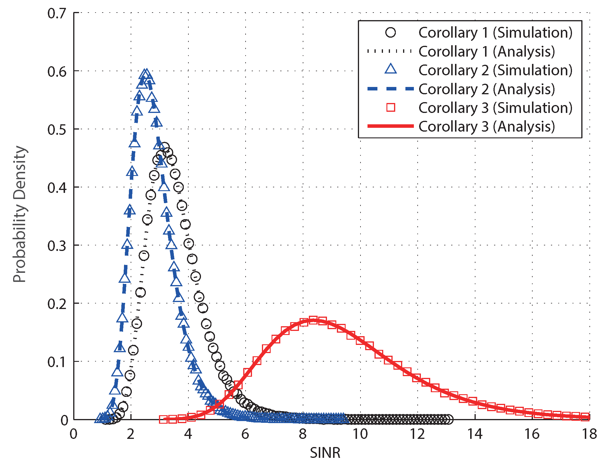
Figure 1, the analytical PDFs of the SINR in the corollaries are compared with the simulation results, where
,
,
dB, and
. The symbols represent the simulation results, and the lines depict the analytical results. From
Figure 1, the derived PDFs match well with the simulation results.
From
Figure 2,
Figure 3,
Figure 4,
Figure 5,
Figure 6,
Figure 7,
Figure 8 and
Figure 9, simulation results for the ergodic sum rates and scheduling gains of user selection algorithms as well as the variances of individual rates and sum rates are shown. The margin of error considering the 95% confidence interval for each point is about
at maximum.
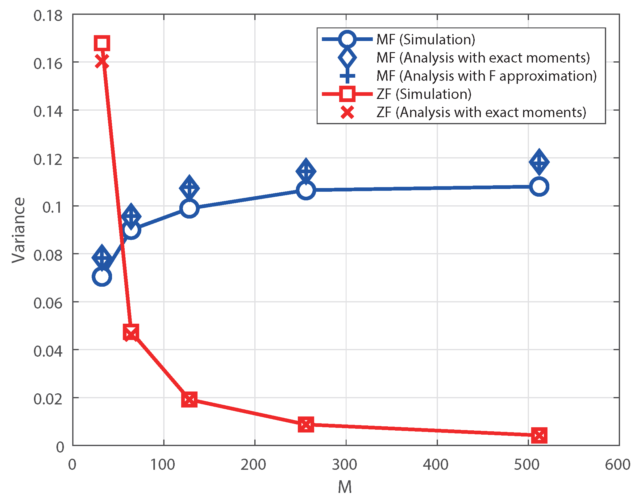
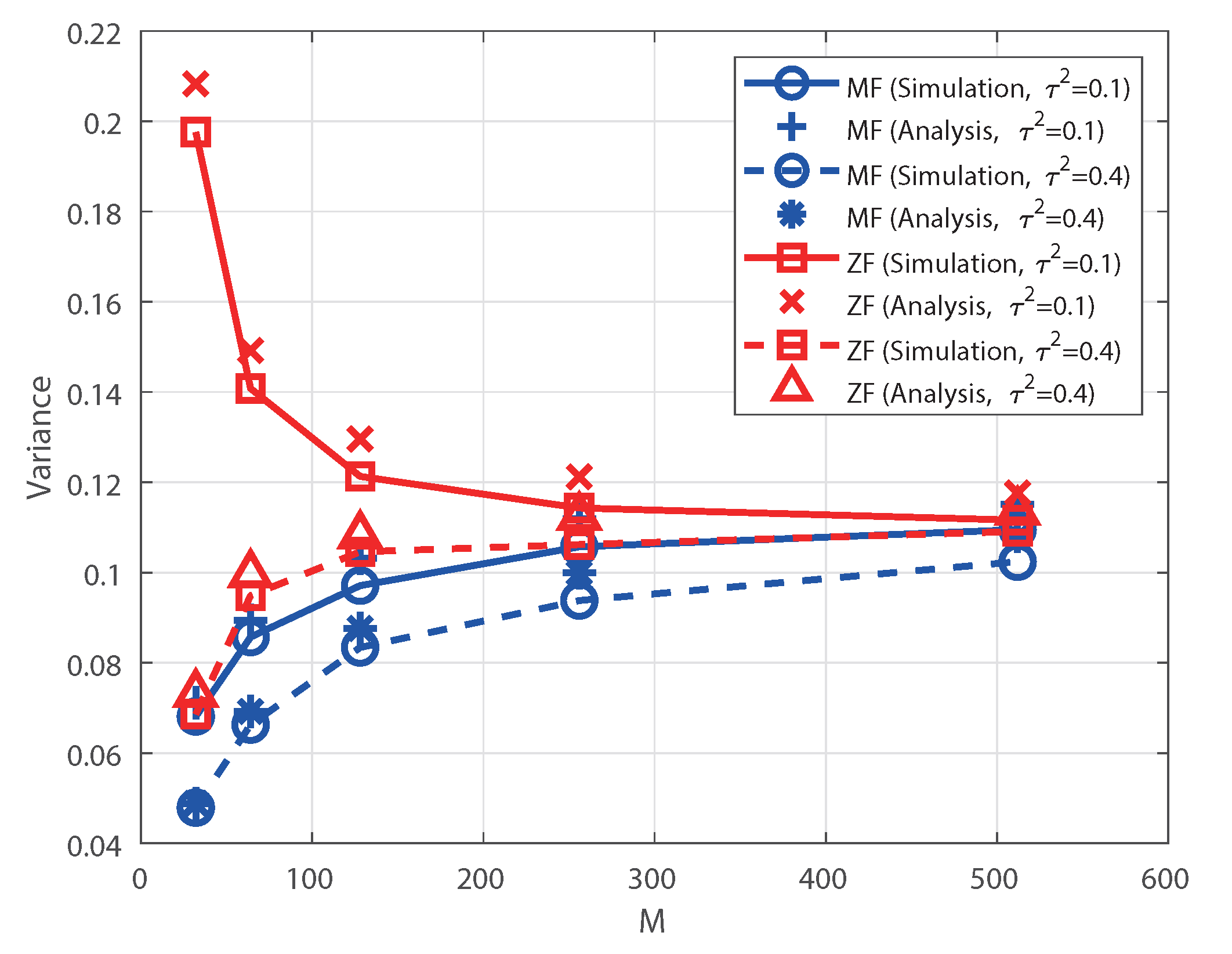
Figure 2 shows the variances of individual rate under perfect CSI according to
M when
and
dB. For the MF receiver, two analytical results are considered: (7) after substituting the exact
and
obtained by the MGF in Corollary 1, and (12) obtained by the F approximation. For the ZF receiver, the analytical result corresponds to (14). For the MF receiver, it is observed that the analytical results with the exact moments and F approximation are almost the same. The difference between the simulation and analytical results is due to neglecting the higher-order moments of SINR in the Taylor series expansion. Therefore, we can confirm that the variance of the MF receiver increases while that of the ZF receiver decreases as
M increases. That is, under perfect CSI, the MF receiver does not exhibit the channel hardening phenomenon unlike the ZF receiver, as predicted.
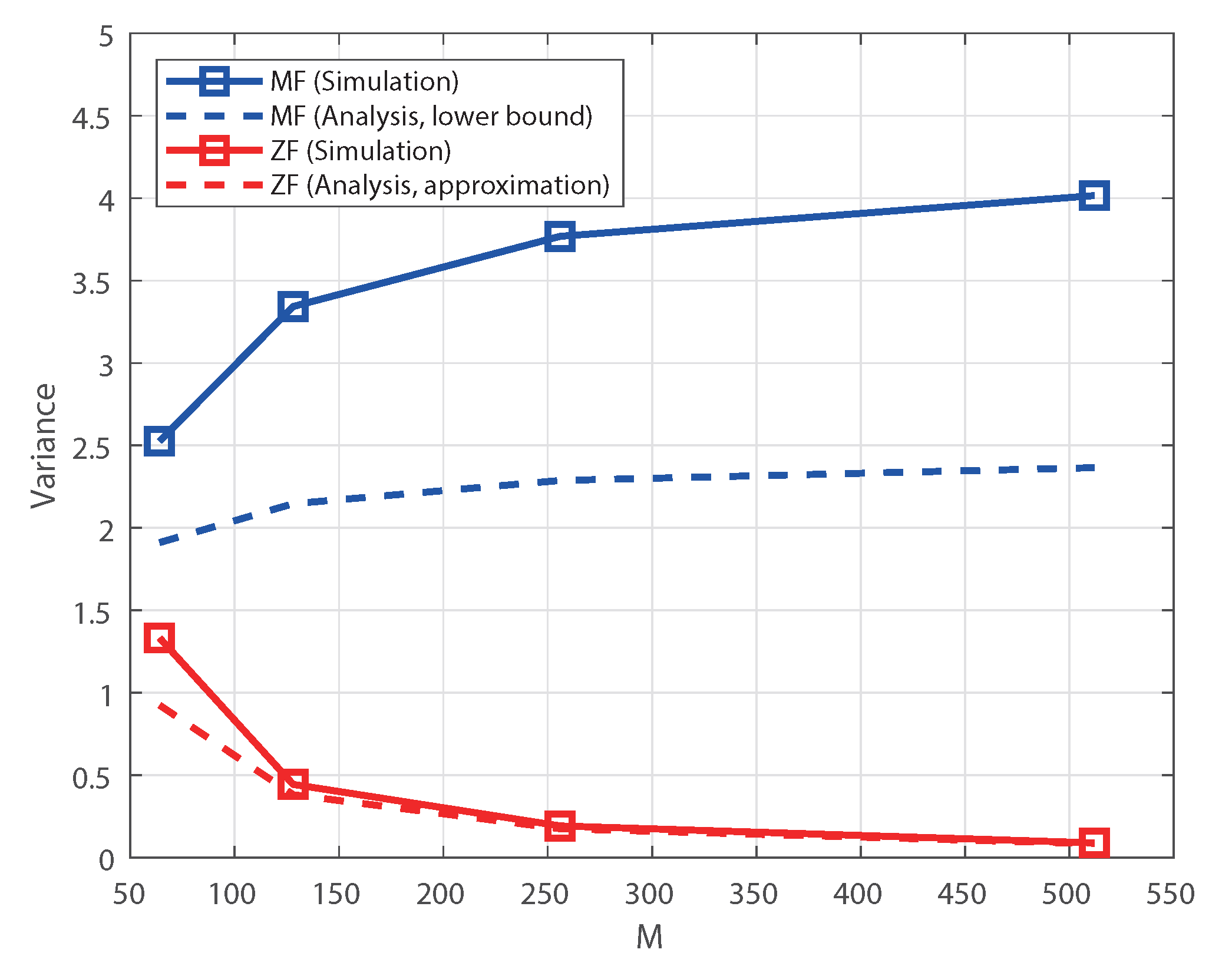
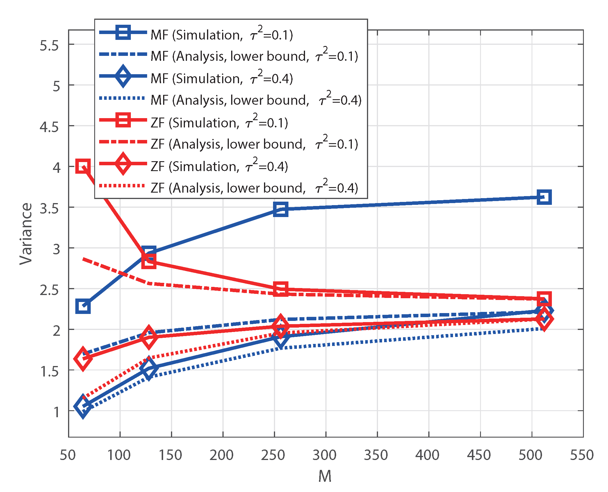
Figure 3 shows the variances of the sum rate under perfect CSI as a function of
M when
and
dB. For the MF receiver, the lower bound in (17) is represented; for the ZF receiver, the approximation in (18) is represented. Similar to the case of individual rate, the variance of the MF receiver increases, while that of the ZF receiver decreases as
M increases. As demonstrated by the analysis, the sum rate of the ZF receiver still exhibits the channel hardening effect.
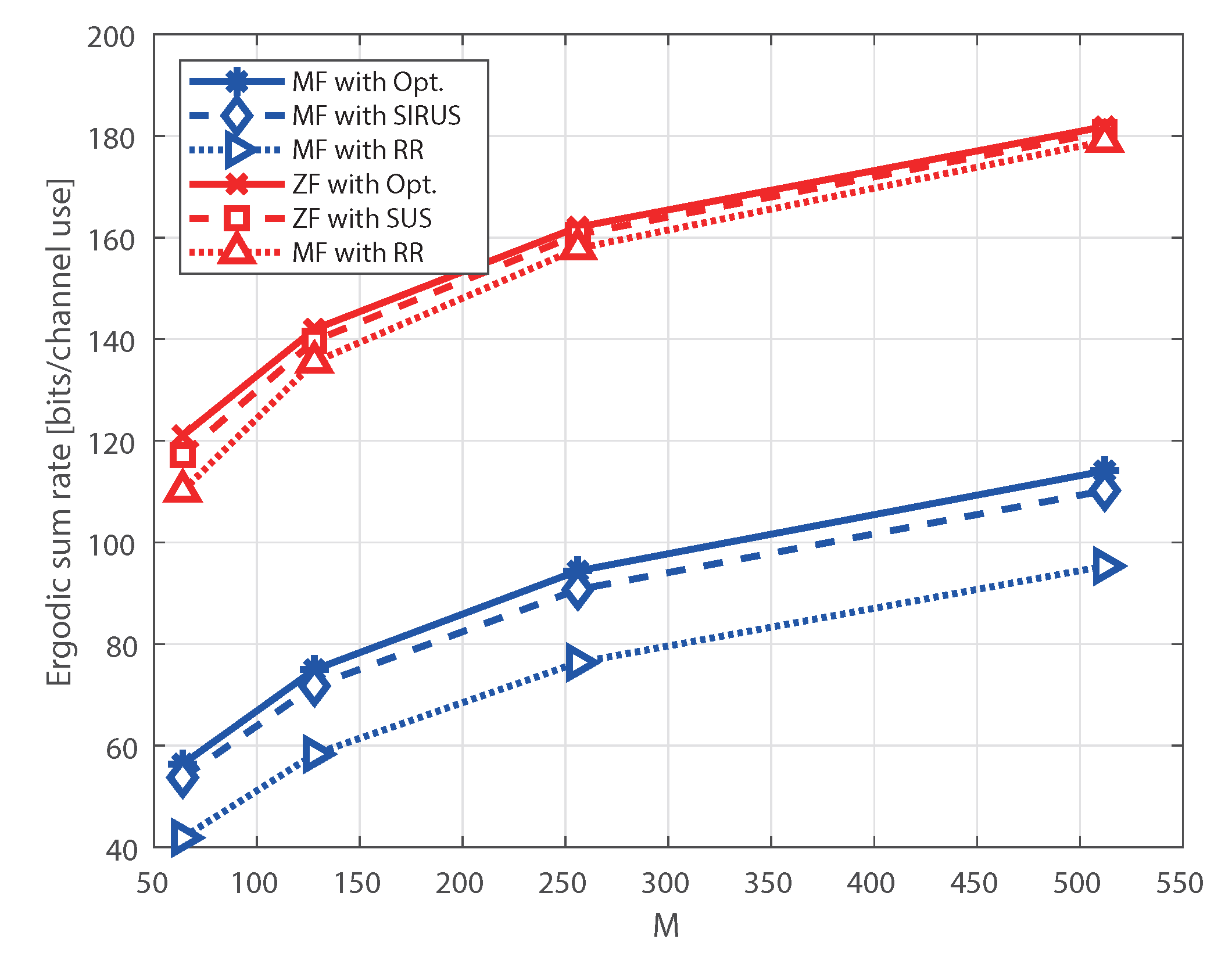
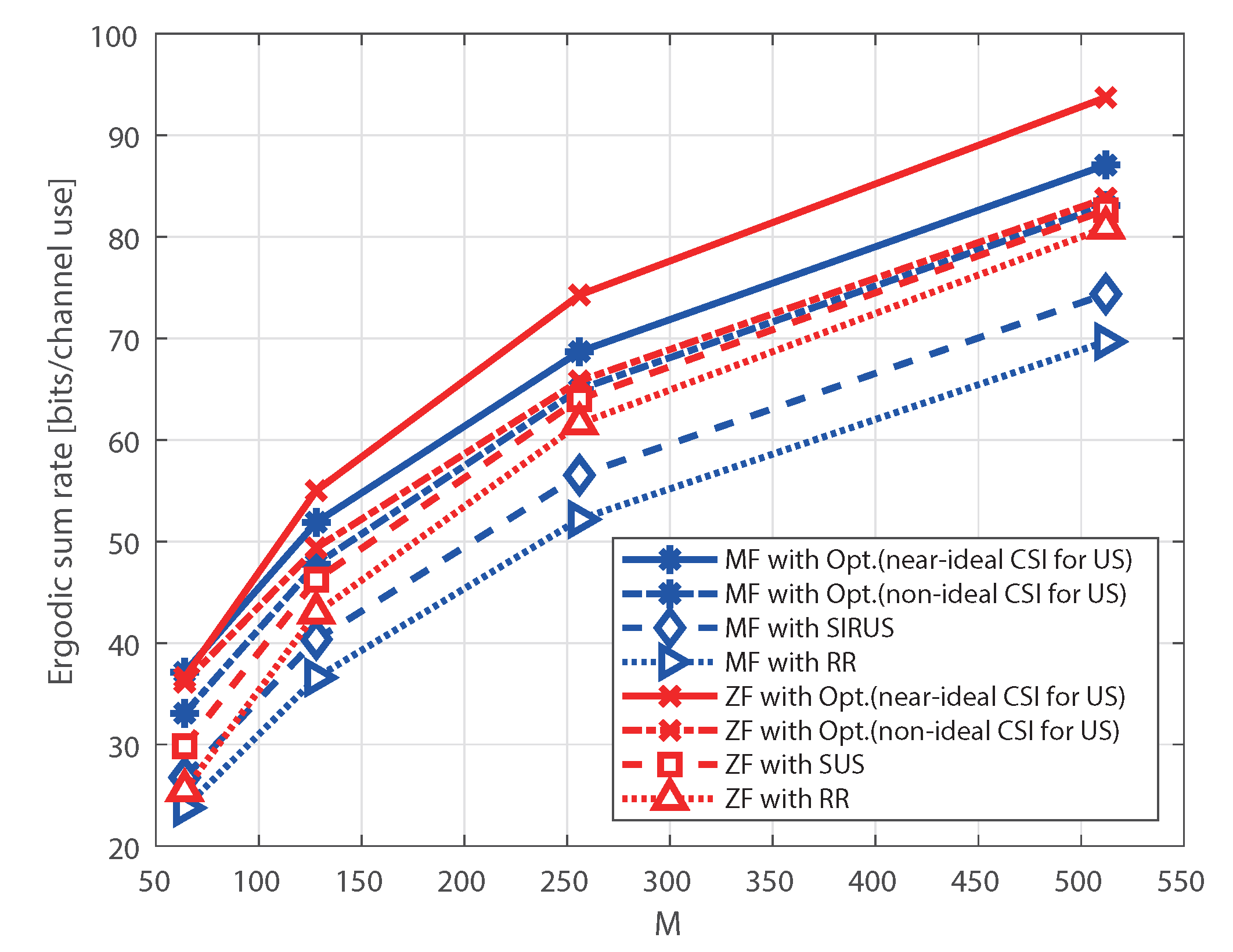
Figure 4 illustrates the ergodic sum rate as a function of
M according to the user selection algorithm at the BS under the assumption of perfect CSI, where
,
, and
dB. For the MF receiver, we consider SIRUS [
14], which is proposed for MF-based massive MIMO systems. In SIRUS, a user who generates the maximum SIR among the remaining users is sequentially selected in a greedy manner until the number of selected users becomes equal to
K. For the ZF receiver, we consider SUS [
13], which is designed for the ZF to maximize the sum rate. In SUS, a user set with near-orthogonal channel vectors is selected in the greedy manner. For comparison, the results of round robin (RR) scheduling and the achievable maximum sum rate in (15), i.e., optimal user scheduling, are presented. The RR scheduler selects the users randomly; hence, no scheduling gain occurs. Meanwhile, the maximum sum rate in (15) can be realized when an optimal user selection algorithm based on an exhaustive search is employed. Therefore, the simulation of the computational complexity of the optimal scheduler is infeasible; thus, the analytical results of (15) are shown, rather than the simulation results. In addition to the ergodic sum rate shown in
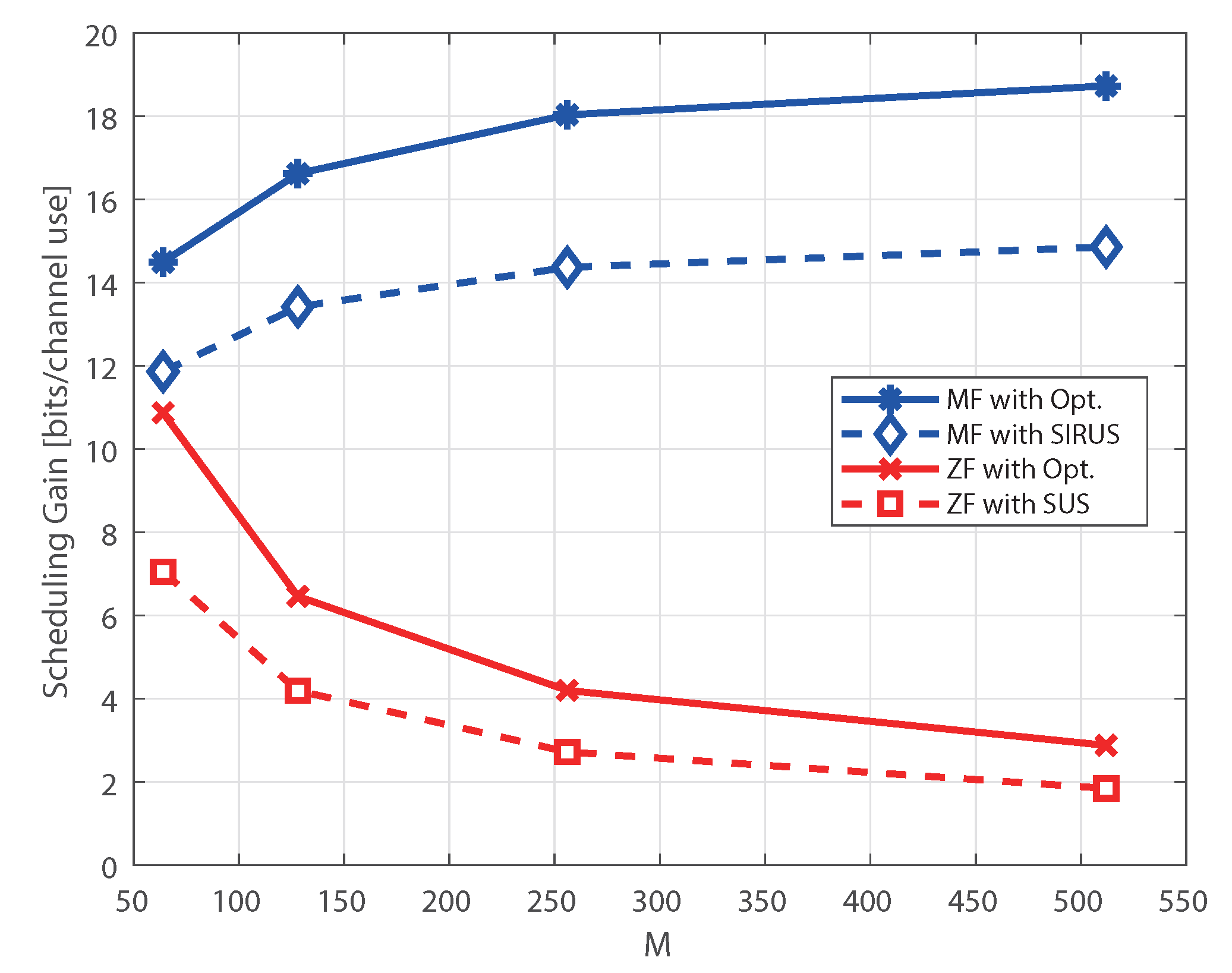
Figure 4, we plot the corresponding scheduling gain as a function of
M under perfect CSI in
Figure 5, where the simulation environment is equivalent to that in
Figure 4. In
Figure 5, the scheduling gain is defined as the performance gain of a specific user selection algorithm compared to RR in terms of the ergodic sum rate.
As shown in
Figure 4 and
Figure 5, the performance gap between the SUS and RR of the ZF receiver decreases as
M increases. This is because the variance of the sum rate decreases for the ZF receiver for a large
M. For the MF receiver, the gain of SIRUS increases and maintains a constant positive performance gap compared to the RR scheduler as
M increases. However, the performance gap between the SUS and RR of the MF receiver shrinks as
M increases, although the variance of the MF receiver increases. That is, for massive MIMO systems with SUS for the MF receiver, multiuser diversity gain is not sufficiently obtained compared to SIRUS. This implies that the user scheduling algorithm should be carefully chosen according to the types of receivers to fully utilize the multiuser diversity. From the simulation results, we can conclude that user scheduling is more important for the MF receiver than for the ZF receiver in massive MIMO systems under perfect CSI, as analyzed in
Section 3.
Hereafter, the simulation results under imperfect CSI are presented from
Figure 6,
Figure 7,
Figure 8 and
Figure 9. In
Figure 6, the variance of the individual rate under imperfect CSI is presented as a function of
M, where
,
, and
dB. For simplicity, the analytical results of the F approximation are omitted in
Figure 6. As demonstrated by the analysis for the MF receiver, the variance of the individual rate always increases, regardless of
. However, for the ZF receiver, the variance of the individual rate decreases when
and increases when
, according to
M. Therefore, it can be observed from
Figure 6 that the imperfectness of CSI affects the channel hardening effect for the ZF receiver. Furthermore, under imperfect CSI, all variances of the individual rate converge to a constant value as
M increases.
Figure 7 shows the variance of the sum rate under imperfect CSI as a function of
M, where
,
, and
dB. For the analytical results, the lower bounds (26) and (27) are shown for the MF and ZF receivers, respectively. Similar to the results in
Figure 6, the scaling law on the variance of the sum rate with
M for the MF receiver does not change, regardless of
, while that for the ZF receiver tends to change depending on
.
Figure 8 represents the ergodic sum rate as a function of
M with the user selection algorithm at the BS, where
,
,
dB and
.
Figure 9 depicts the corresponding scheduling gain. The cases of a small
are not presented for simplicity. As explained in
Section 4, we consider two scenarios for CSI availability for user scheduling at the BS, namely non-ideal CSI and near-ideal CSI. The exhaustive search for the optimal user selection algorithm uses the exact SINR formula in (4) as the selection metric; thus, the CSI availability for user scheduling only affects the scheduling gain for the optimal user selection algorithm. Conversely, SUS and SIRUS are not influenced by the CSI availability for user scheduling because the user selection metrics are calculated using the estimated channel. Moreover, the RR scheduler is not affected by the CSI availability for user scheduling because of the random user selection.
From
Figure 8 and
Figure 9, it is observed that the scheduling gain for the MF receiver increases as
M increases, regardless of both the user selection algorithm and CSI availability for user scheduling. Simply, the scaling law for the MF receiver does not change depending on the user selection algorithm and CSI availability for user scheduling. However, the scheduling gain for the ZF receiver shows different scaling laws with
M depending on the two factors. For the ZF receiver, it is observed that the scheduling gains for (i) optimal scheduler with non-ideal CSI for user scheduling and (ii) SUS decrease as
M increases, while that for an optimal scheduler with near-ideal CSI for user scheduling increases with
M. This implies that if near-ideal CSI is available for user scheduling, full multi-user diversity gain from the fluctuation of the sum rate can be achieved under the optimal user selection algorithm for the ZF receiver. However, if non-ideal CSI is available for user scheduling, the achievable scheduling gain is limited, even if the optimal user selection algorithm is employed. If a typical low-complexity user selection algorithm, such as SUS, is employed, the scheduling gain for the ZF receiver decreases as
M increases, even though the variance of the sum rate increases with
M. Therefore, for a large
, the benefit of user scheduling for the ZF receiver disappears under imperfect CSI provided that the user scheduling is far from optimal, and only non-ideal CSI is available for user scheduling, as analyzed in
Section 4.


